ic copy naval postgraduate school monterey, california=onvection immersion cooling of a three by...

IC FILE COPY

NAVAL POSTGRADUATE SCHOOLMonterey, California

STAT~y 4 AD-A219 819

0S7GR AD13

THESIS

NATURAL CONVECTION FROM AN ARRAYOF RECTANGULAR PROTRUSIONS IN AN

ENCLOSURE FILLED WITH DIELECTRIC FLUID:EFFECTS OF BOUNDARY CONDITIONS,

FLUID PRANDTL NUMBER,AND SELECTIVE POWERING.

by

Mark E. Powell

September 1989

Thesis Advisor: Yogendra Joshi

Approved for public release; distribution is unlimited

DTICELECTE.MAR 2 9 IWO 1

t~l B ID39(0o

SEC~R TsY CLA iT 1 0N 0F T HS Pc,

REPORT DOCUMENTATION PAGE,a REPORT SEC(.RIY CLASSFCATION 'Ib RESTRICTIVE MARXcINGS

Unclassified________________ _____

2j SFCR TY C ASSII ICATION AuTmOR TV 3 DISTRiSUTION/AVAILAILiTY OF REPORT

1, 1iASC!O O~CA'GSOL Approved for public release;, )DitaS A AT0% OWNRA'NC SHEDLEDistribution is unlimited

4 -- RFORV NG ORGANZJATION REPORT NUMBIER(S) S MONITORING ORGANIZATION REPORT NUMBER(S)

6a NAVE OF PERFORMING ORGANIZATION 6t) OFFCE SYMBOL ?a NAME OF MlON'rOR.NG ORGANZATION(if EDDocable)

Naval Postgraduate Schooll Naval Postgraduate School6& AOT)RFSS .CJt' State afld ZIP Code) 'b ADDRESS (Cry State and ZIP Code)

Y:onterey A 34-00Monterey CA 934-5000

S.a NAM)v : F - JTDNG SPONSORNC, (Sb OFP CE SYMABOL 9 PROCUREMENT NSTR VMENr DEN' F (ArI iO k-,MBER

8zAOR S (C.r Srte and ZIP Code) 10 SOvjRCE OF F N~iNC NJMNBE RS

PROGRAM IPROECT 7 AS'( AORK Nt17ELEMENT NO NO %O ACCESS (11' No

-~'ocSenr C~s~caT~Natural Convection from an Array of Rectangular Prot-rus:zons in an Enclosure -illed w-,ith Dielectric z-luid; Effects of_ Boundary

oniiicn, Fuid rantl umb: ~dCcl~ti~ 7tn4~Mark F.Powell

- -.... iL'.R* * ~' - 4 DATE OF RE PORT iYed' Month Day) -;t C ( O.NT

Master s Th Setember l19B_ 771o~(OS ' C-:E J8 SUB kc, 'ERY~S 'caritnueo IF V s.a-y antd 'der.t*. byPIC(Ar rnjmber)

Qr -- T- - irecL Immersion, "altura7 tonvection ooling,'4- ,B)OP ielectric Liouid Protrusions;'nclos-ure'Siuaeircuit Board;* Convective Heat Transfer .

3 ASR( 'Orlf',ue On levtre If mecepsan ano oocnif by biok mumnbe,)Ane6xperimirental investigation has been conducted to further examin'e Natural=onvection Immersion Cooling of a three by three array o -F heated protrusiors

in a rectang7ular chamber filled with dielectric fluid.E ach rectangular prol-rusion geometrically modelled a 20 pin dual inline package.Input power toeach component varied from 0.1 to 3.0 W.-The purpose of this study was to examine the effects of the following para-meters for the range of power levels selected:1)Top and bottom boundarytemperatures;2)Selective powering of components;3)Changes in the 7luid?ranldtl number.The data were obtained as component surface temperatures. These were sub-seauently presented in terms of appropriate non-dimensional parameters. Aspcart of the ov.,erall investigation, flow visualjzation results are alsopres-ented f-or selected conditions. <, r

I ~ .1 -~A AS-, " 0- ABSRA?2tARACAC SECURITY CLASSFiCA'iONE:-% f%A NTE, C3 SAME AS APT OOTC _SERS UnclassifiedR

"a ')F RE S O L~BE I.D D,_A 22b TELE P-ONE (Inlude Anca Code) I 2 0;F (I S%9

Prcfessor Yo-ndr-a Jnohi I(4og) 4(_L4n,f 0- 9JI00 FORM 1473.! 0)8 APR pa (i c -ay be .ied u-11- evrP8~sld SEu

T LST(TCN > PACFAl. Othe' #d t~om afe Obiolfe Unclassified

i

Approved for public release; distribution is unlimited

Natural Convection from an Array of Rectangular Protrusions in anEnclosure Filled with Dielectric Fluid: Effects of Boundary Conditions, Fluid

Prandtl Number, and Selective Component Powering.

by

Mark E. PowellLieutenant, United States Navy

B.S., University of Oregon, 1978

Submitted in partial fulfillment of therequirements for the degree of

MASTER OF SCIENCE IN MECHANICAL ENGINEERING

from the

NAVAL POSTGRADUATE SCHOOL

September 1989

Author: ' - " z-

Mark E. PowellApproved by: / -

Yogendra Joshi, Thesis Advisor

Department of Mechanical En neering

ABSTRACT

An experimental investigation has been conducted to further examine natural

convection immersion cooling of a three by three array of heated protrusions in a

rectangular chamber filled with dielectric fluid. Each rectangular protrusion

geometrically modelled a 20 pin dual-inline-packagc. Inrput power to each component

varied from 0.1 to 3.0 W..

The purpose of this study was to examine the effects of the following

parameters for the range of power levels selected:

1). Top and bottom boundary temperatures.

2). Selective powering of components.

3). Changes in the fluid Prandtl number.

The data were obtained as component surface temperatures. These were

subsequently presented in terms of appropriate non-dimensional parameters. As part

of the overall investigation, flow visualization results are also presented for selected

conditions.

Aooession For

NTIS GRA&IDTIC TAB 0Unannounced 0Just if eat ton

Distribution/

Availability Codes-, vail and/or

K Dist Special

'g 4<( ' Ilk"

TABLE OF CONTENTS

I. IN T R O D U C T IO N ............................................................................ 1

A. DESCRIPTION OF PROBLEM ...................................................... 1

B. STUDIES OF NATURAL CONVECTION COOLING OF

C . O B JE C T IV E S .......................................................................... 4

II. EXPERIMENTAL SET UP ........................................................... 6

A . A PP A R A T U S ........................................................................... 6

B. APPARATUS PREPARATION PROCEDURE ............................. 13

C. DATA ACQUISITION PROCEDURE ....................................... 13

D. DATA ANALYSIS .............................................................. 14

1. Heat Transfer Coefficient ............................................... 14

2. N usselt N um ber ........................................................... 14

3. Rayleigh Number ........................................................ 15

iv

III. R E S U L T S ................................................................................. 17

A. HEAT TRANSFER MEASUREMENTS ..................................... 17

1. Verification of Earlier Data ............................................ 17

2. Effects of Chamber's Top and Bottom

Surface Boundary Variations ......................................... 20

3. Variation in Fluid Prandtl Number .................................. 30

a. Numerical Correlation ........................................... .36

4. Selective Powering of Components .................................. 39

B. FLOW VISUALIZATION ...................................................... 45

1. Flow Patterns with No Power Input ............................... 45

2. Flow Patterns Powered at 0.1 W .................................... 49



IV . C O N C L U S IO N S ........................................................................ 6 1

V. RECOMMENDATIONS ........................................................... 62

V

APPENDIX A SAMPLE CALCULATIONS ............................................ 63

APPENDIX B UNCERTAINTY ANALYSIS ........................................ 72

APPENDIX C EXPERIMENTAL NUSSELT TO RAYLEIGH

NUMBER RELATIONSHIP SPECTRUM ........................ 79

LIST OF REFERENCES ................................................................... 89

INITIAL DISTRIBUTION LIST ............................................................ 91

vi

LIST OF SYMBOLS

Symbol De.s.rilti.n Units

A Area m 2

Atotal Total Exposed Surface Area m2

Cp Specific Heat J/Kg *C

emf Thermocouple Voltage mV

g Acceleration due to Gravity m/s2

Grf Flux-based Grashof Number Dimensionless

Grt Temperatu:e based Grashof Number Dimensionless

h Heat Transfer Coefficient W / m2 °C

kf Fluid Thermal Conductivity W / m*C

L Characteristic Length m

LI Component Length in the Vertical m

Direction

L2 Summation of the Ratios of the m

Component Fluid Exposed Areas to

their Perimeters

Nu Nusselt Number Dimensionless

Nul Modified Nusselt Number with Dimensionless

with Length Scale LI

Nu2 Modified Nusselt Number with Dimensionless

with Length Scale L2

vii

Pr Prandtl Number Dimensionless

Qin Power Input to the Heaters W

Q1oss Rate of Loss by Conduction W

Qnet Net Power Dissipated by the Heater W

Rc Total Thermal Resistance C/ W

Rp Resistance of the Precision Resistor Dimensionless

Raf Flux-based Rayleigh Number Dimensionless

Rat Temperature based Rayleigh Number Dimensionless

Tavg Average of Component Surface °C

Temperature

Tback Back Surface Temperature of the C

Substrate

Tfilm Film Temperature °C

Tsink Average Temperature of the Heat °C

Exchangers

U Uncertainty Value Various

Vin Input Voltage Volts

Vh Voltage Across the Heaters Volts

cX Thermal Diffusivity m2 / s

3 Thermal Expansion Coefficient 1 /°C

p Density Kg / M3

1) Kinematic Viscosity m2 / s

viii

I. INTRODUCTION

A. DESCRIPTION OF THE PROBLEM

The final constraint for the continuing development of future generations of high

speed, very large scale integration (VLSI ) technologies may simply be the lack of

effective heat dissipation. In order to meet acceptable system reliability criteria,

junction temperatures of modem electronic components must be maintained below

1250 C. For every 20" C decrease in junction temperature, the long term reliability

improves on the order of 50% [Ref. 1].

Several solution options have been proposed and described in detail [Ref.2&31.

However, in the advent of the 1990's, "Super Chips" powered to 50 W with

respective heat fluxes ranging from 50-250 W/cm 2 will saturate the capabilities of

forced air cooling technologies [Ref. 4]. Therefore, applications of direct immersion

cooling have been the focus of several experimental and computational studies in

recent years: Simons and Moran (1977); Bar-Cohan (1983); Simons and Chu(1985);

and Joshi et. al.(1989). Single Phase liquid cooling may in general involve natural,

mixed or forced convection. Natural convection in dielectric fluids as a cooling

mechanism promises to be a potentially attractive technique for thermal control of

micro-electronic components/systems. Desirable characteristics include, attainable high

heat transfer rates, low noise, high reliability, and simplicity of design.

Unfortunately, direct immersion cooling applications have only been limited to mixed

or forced convection in a Cray-2 Supercomputer.

B. STI'PiES OF NATURAL CONVECTION COOLING OF

ELECTRONIC DEVICES

Direct immersion cooling of discrete heat source using both forced and natural

convection was first examined by Baker[ Ref. 5]. Air, Freon 113 (Prandtl number

(Pr) = 3.9 ) and Dow Coming #200 silicone dielectric liquid (Pr = 126 ) were used.

Results indicated that natural convection direct liquid cooling was three times more

effective than natural air convection cooling. Also, the analysis showed that the heat

transfer coefficient isapproximately proportional to the cube root of the reciprocal of

viscosity. Consequently, the use of a lower viscosity fluid would increase the heat

transfer coefficient significantly.

In a following investigation, Baker [Ref. 61 demonstrated that liquid immersion

techniques can effectively cool small heat sources. The study showed the effect of

heat source size on the heat transfer coefficient with both natural and forced

convection in two different liquids. Results indicated an order of magnitude increase

in the heat transfer coefficient as heat source size decreased from 2.0 to 0.01 cm 2.

Park and Bergles [ Ref. 7 ] examined natural convection with discrete flush

mounted protruding heaters of 5 and 10 mm height and widths in the range of 2-

70mm, in water and Freon 113. This study indicated that the heat transfer

coefficient increased with decreasing width, with the effect greater in Freon 113

than water. Data also indicated, that the heat transfer coefficients, for various array

configurations, were higher in the upper heaters than the lower heaters, and as the

2

distance between the heaters increased so did the heat transfer coefficients.

Additionally, heat transfer coefficient for a single protruding heater was about

15% higher than that for a flush surface.

Keyhani et. al. [Ref. 8] investigated the buoyancy driven flow and heat transfer

in a vertical cavity with discrete flush heat sources on one vertical sidewall. The

enclosure chamber configuration had 11 alternatively unheated and flush mounted

rows of isoflux strips. Two immersion coolants were used, water and ethylene-

glycol ( P- = 150 ).

Chen et. al. [Ref. 9] investigated natural convection heat transfer in a liquid

filled rectangular chamber with 10 protruding heaters from one vertical wall. The top

chamber surface was maintained at a uniform temperature and acted as a heat sink.

All other chamber surfaces were unheated. Two fluids, distilled water and ethylene

glycol were used as immersion coolants. Results indicated that, at low Rayleigh

number, the bottom heater had the highest heat transfer coefficient. At high Rayleigh

niumbers, the top heater had the highest heat transfer coefficient. Flow visualization

was also conducted.

Liu et. al. [Ref. 10] presented a finite difference numerical study of natural

convection flow in a rectangular chamber, with a 3 by 3 array of uniformly heated

protrusions mounted on ani otherwise adiabatic vertical wall. The enclosure was

filled with Fluorinert FC-75 dielectric fluid. The top and bottom were maintained at

uniform temperatures while the other boundaries were adiabatic. Results of this

numerical study were presented for chamber widths of 18 and 30 mm.

3

Kelleher et. a] [ Ref. 11] investigated natural convection flow and heat transfer in

a water filled rectangular chamber with a long heater protruding from one vertical

insulated wall. Visualizations indicated a dual celled flow str -'ure. The "Buoyancy

driven" upper cell accounted for a majority of convective heat transfer. A "shear

driven" lower cell was also found, in which the fluid motion arises due to viscous

drag from the upper cell.

Lee et. al. [ Ref. 121 confirmed the distinct flow patterns by accompanying two

dimensional numerical computations.

Joshi et. al[ Ref. 13] investigated natural convection cooling of a 3 by 3 array

of heated protrusions in a rectangular chamber filled with FC-75 dielectric fluid.

Results indicated that at low power levels ( 0. 1 W ), flow structure was determined

primarily by the thermal Boundary Conditions of the chamber. On increasing the

power levels (0.7 to 3.0 W ) an upward flow developed adjacent to each column of

components. The flow away from the elements showed strong three dimensional

time dependent behavior with increasing thermal input. Component surface

temperatures were used to arrive at non dimensional heat transfer correlations.

C. OBJECTIVES

This work is a continuation of Thesis research conducted at the Naval

Postgraduate School. Knock [Ref. 14] studied the effect of the location of a single

protruding heater using water in an enclosure. Pamuk [ Ref. 15] first studied the

heat transfer characteristics of a nine protrusion array immersed in a dielectric fluid

in an uninsulated enclosure. Hazard [Ref. 16] investigated natural convection liquid

cooling of a vertically oriented simulated component array with and without a

4

shrouding wall. Benedict [Ref. 17] arranged a horizontally oriented three by three

simulated array that investigated various power level inputs, flow visualization,

and correlation of data using Nusselt and Rayleigh numbers. Finally, Torres [Ref.18]

re-oriented the three by three simulated component array vertically and followed up

on Benedicts' work.

Investigation objectives are five fold:

1). Examine the effects of different chamber top and bottom surface

Boundary Conditions.

2). Detailed investigation of the effects of various Prandtl number dielectric

fluids.

3). Determine effects of selectively powered components.

4). Investigation to the plausibility of determining a single correlation for all

data.

5). Flow Visualization

5

II EXPERIMENTAL SET UP

A. APPARATUS

This study is a continuation of past experiments conducted at the Naval

Postgraduate School: Knock [ Ref. 14]; Pamuk [ Ref. 15]; Hazard [ Ref. 161; Benedict

[ Ref. 17]; and Torres [ Ref. 18]. The purpose of this investigation is to further

examine natural convection heat transfer from a 3 by 3 element array of simulated

electronic components. The specific aspects investigated were: (i) the effect of fluid

Prandtl number on heat transfer; (ii) the effect of varying the top and bottom

surface boundary conditions; and (iii) Component temperatures resulting from

selective powering.

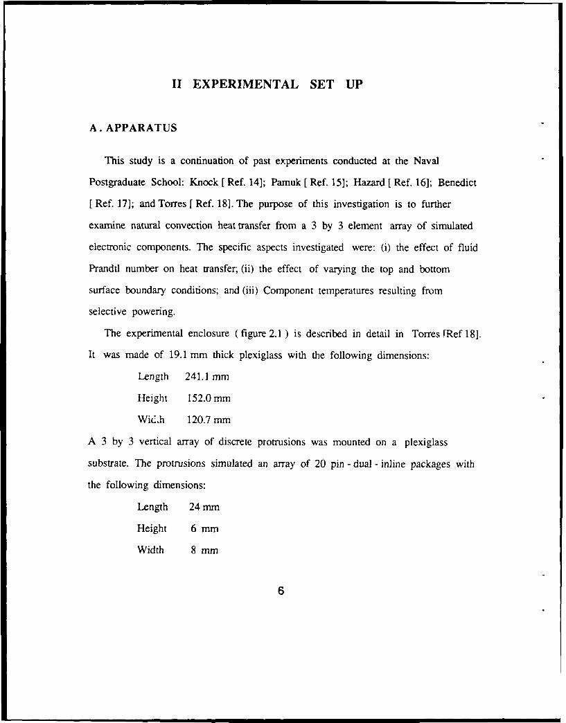
The experimental enclosure (figure 2.1 ) is described in detail in Torres [Ref 18].

It was made of 19.1 mm thick plexiglass with the following dimensions:

Length 241.1 mm

Height 152.0 mm

Widhh 120.7 mm

A 3 by 3 vertical array of discrete protrusions was mounted on a plexiglass

substrate. The protrusions simulated an array of 20 pin - dual - inline packages with

the following dimensions:

Length 24 mm

Height 6 mm

Width 8 mm

6

EE

in

0iF clN

x xI

xC xI

34 - -

E) in CV

a)

X0

El

NXQ

The component dimensions are identical to those investigated by Liu et. al.

[Ref 10], Pamuk [Ref. 16], Benedict [ Ref. 17], and Torres [ Ref. 18] in order to

enable comparisons of experiments and numerical finite difference computations.

The components were oriented with their largest dimension being vertical (figure

2.2 ), with the plexiglass surface containing the protrusions forming a vertical

boundary the dielectric inert fluid.

The top and bottom surfaces of the chamber are 3 mm thick Aluminum plates

allowing almost uniform surface temperature. In order to maintain the prescribed

temperatures, two heat exchangers with individual chilled water circulatio, b,,ths

are attached. Modifications (figure 2.3 ) were made to the top heat exchangers'

inlet and outlet headers described in Benedict [Ref. 17] to allow better flow

distribution of coolant.

The protrusions were heated using foil heaters attached to the component bases

using a high thermal conductivity epoxy ( Omega Bond 101). The heating elements

contains a network of Iconel foil mounted on a Kapton backing, and were

powered by a 0-40 Volt 0-1 Amp D.C. power supply. The strip heaters were

connected in series with 2 Ohm precision resistors. This allowed the measurement

of the current. The current was multiplied by the strip heater measured voltage to

compute the component power input.

Temperatures at the center of each exposed protrusion face were determined

using 0.127 mm diameter embedded Copper Constantan thermocouples (figure 2.4).

All thermocouples were connected to a Hewlett-Packard Data Acquisition System (

HP-3497 ) controlled by a Hewlett-Packard micro-computer ( HP-9826) shown in

Figure 2.5.

8

UE3E

C-i

E E U U

EEro~1 0

EN

00

0

E~t

inU

I 6q

PLEXIGLASS &35MM 158mmCASING ~4-3.17 mm

Ia) 0 .25.4 mm

1P 6.35rm

-1905 -4 4 4.45 mm

120.65 mm

ALUMINUM PLATE-

TOP HEAT

EXCHANGER

BOTTOM HEAT

EXCHANGER

MODIFICATIONS TO COOLANT

31.75mm 5-E0

25.4 nm

- 62.55 mm

Figure 2.3 Heat Exchangers()Cross Sectional View; (b) Isometric View;

(c) Inlet and Outlet Headers10

.51 R (4-PLACES)

II.9 4-4HOLE

p :,23.88"

- 6.22

ITOP6.10 " VIEW

.. SIDE

7.87 . L VIEW

" 6.10

" THERMOCOUPLE WELLS

I .- " /ISOMETRIC

ALL DIMENSIONS IN MILLIMETERSI

Figure 2.4 Heating Element and Thermocouple Locations

11

0

wE

Ch D

0 Q.,

0-0

U:.

121

B. APPAAATUS PREPARATION PROCEDURE

As delineated in Benedict [Ref. 17], once the apparatus was sealed, the chamber

was filled with the desired dielectric fluid by using the attached reservoir assembly.

It was essential to manipulate the chamber to eliminate the formation of air bubbles

within the chamber. The heat exchangers were then independently adjusted and

maintained to the desired temperature.

C. DATA ACQUISITION PROCEDURE

Prior to energizing the components, a trial scan was made each time to verify

proper operation of all component and heat exchanger thermocouples.

Once the trial run was satisfactorily completed, the desired component power

level was set on the power supply. Steady state conditions were assumed when

the thermocouple outputs varied by a maximum of 0.5 C, with the majority

varying by less than 0.2° C during three successive scans at 15-30 minute time

intervals.

Time needed to achieve steady state increased with the viscosity and Prandtl

number of the dielectric fluid. For dielectric FC-75 (Pr = 3G ) it took approximately

3-5 hours to achieve steady conditions while for higher viscosity dielectric FC-71

( Pr = 1400 ) a minimum of 8 hours was needed to achieve steady state

conditions.

Once steady state conditions were achieved data were recorded and subsequently

processed. The thermocouple emf s were converted into temperatures, which were

used in generalizing the thermal characteristics described next.

13

The Data Acquisition software program ACQUIRE was the same as used by

Pamuk [Ref. 16], Benedict [Ref. 17] , and Torres [Ref. 181 with modifications in the

different dielectric fluid properties

D. DATA ANALYSIS

1. Heat Transfer Coefficient

Heat transfer coefficients in this study were calculated based on an average

component surface temperature in the following manner:

h = Qnet / Atotai ( Tavg - Tsi)

where

Qnet Net rate of energy transferred to the fluid per element. Calculatedas the net input power rate minus the conduction loss throughthe back of substrate.

AtoW - Total wetted surface area of a specific electronic component

Tavg The temperature average over the exposed area divided by thefive wetted component faces, or mathematically

Tavg = XAiTi]/Ai

Tsi - Average heat exchanger temperature

2. Nusselt Number

In order to compare results from this experiment with other studies, a non-

dimensional representation of the heat transfer performance, the Nusselt number was

defined as:

14

Nu = hL/kf

where

h -Convective heat transfer coefficient

L -Height of each component

kf-Thermal conductivity of the fluid

we note that the fluid properties were taken as a function of the average film

temperature calculated as:

Tf = (Tavg + Tc ) / 2

for each component.

3. Rayleigh Number

A non-dimensional Rayleigh number based on temperature was defined for

this st. v to be:

Rat =Grt Pr

where

Grt (Grashof number ) fm g 13 L3 AT / -o2

Pr (Prandtl number) u /

Using the average surface temperature of the specific component defined

previously yields the following Rayleigh number expression:

Rat =g 13 L3 (Tavg-Tsink)/ 'iac

15

Another Rayleigh number based on the component heat flux was defined

as follows:

Raf=Grf Pr=g 0 LA QneL/kf Aotal u x

The use of these relationships is presented in the Sample Calculations and

Uncertainty Analysis Sections of the Appendices.

16

III. RESULTS AND DISCUSSIONS

A. HEAT TRANSFER MEASUREMENTS

The bulk of the present investigation involved heat transfer measurements at

various power levels to examine effects of variations in top and bottom surface

boundary conditions, fluid Prandtl number, and selective powering of components.

Information on the heat transfer characteristics is presented in terms of

appropriate non - dimensional groups. As in Benedict [Ref. 17] and Torres [Ref. 181,

we identify the Nusselt number ( Nul ) as the inverse of the dimensionless surface

dimensional flow vigor parameter ( see Appendix A Sample Calculations for

derivations ).

1 . Verification with Earlier Data

The starting point of this experimental study was to reproduce results

obtained by Torres [ Ref. 181. Using Dielectric FC-75 and setting the top and

bottom surfaces to 10 °C, the resulting heat transfer data are seen in Figure 3.1.

The corresponding data from Torres [Ref. 18] are seen in Figure 3.2. Comparing

Figures 3.1 and 3.2, good agreement is found for the power levels of 0.1

and 0.7 W.

At 1.1 W we see a somewhat larger spread in the magnitude of the Nusselt

number. However, at the higher power levels, results of this investigation again are

closer in magnitude. Thus an overall satisfactory agreement was found with a

maximum difference of 13 % in the Nusselt number values at any given Rayleigh

number.

17

z C

e.)

C4-I

-U

06

cc.

en,_

Tam aawfrlasfw -

186

z 0

DC3 <+ x C> x 0

0 *

C> E-

-4-

=0-

D04Va

en

19

2. Effects of Varying Top and Bottom Surface Boundary

Conditions

One of the objectives of this investigation was to obtain heat transfer data

using the same dielectric fluid but varying the enclosure top and bottom surface

conditions. In order to examine these effects two sets of plots were generated. The

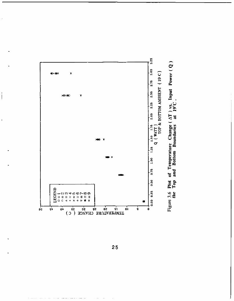
first set (Figure 3.3 to 3.6 )determined the difference between the average

component surface temperature (Ta,,g) and the average heat exchanger temperature (

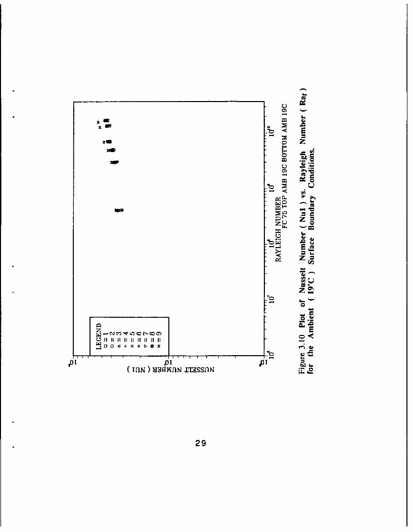
Tsink ) versus the power level (Qin). The second set of plots was a non-

dimensionalization of the same data and (Figures 3.7 to 3.10 )presented the

Nusselt number (Nul ) versus the flux based Rayleigh number (Raf).

Starting with the Standard case of FC-75 with the top and bottom

boundaries set at 15 *C and 10 °C respectively (Figure 3.3 ), we see that at the

lower power levels (0.1, 0.7 W) there is little temperature variation from

component to component. However, as the power level increases, the spread in the

temperature excess levels of the individual components increase, with the middle

column made up of components 4, 5, and 6 ( see figure 2.2 ) has consistently higher

temperatures than the other combinations of rows and columns.

The Verification case (Figure 3.4 )of 10 *C top and 10 °C bottom

boundary temperatures indicated similar trends.

The top 10 °C and the bottom 15 °C case (Figure 3.5 , again show the

same general characteristics as the first two cases. However, the magnitudes of the

temperature excess levels are now significantly lower. This may be due to the

global natural convection flow set up due to the differences between the top and

bottom boundaries.

20

Comm x

CC

0 -

E - cm

0- cc

C

z6

.40~~ 0 +X t

Tw

21

DDO X L

W

o C) C

L) <

E

0

-C

Awx 641

TiOO44 *I~mI

tw669'Z o CT 1 9 o

22

C

o~ u <

sqcc

w~~ 0

23

The last set of measurements was made with the top and bottom

surfaces set to an arbitrary "Ambient" temperature (Figure 3.6 ). Results showed

that at the lower power levels (0.1, 0.7, 1.1, 1.5 W ) the temperature difference

magnitudes of the ambient case were higher than the Standard case and lower at

the higher power levels ( 2.5, 3.0 W).

Reviewing Figures 3.7 to 3.10, an interesting phenomena arises at the

higher power levels. Apparently the displayed effects of the boundary conditions

are insignificant to the Nusselt /Rayleigh number relationship, since the buoyancy

forces produced near the components tend to dominate the circulating flow.

The only major difference in these Figures are the responses at the 0.1 W

power level. Evidently the component energization at these levels has only a weak

influence on the natural circulation of the dielectric fluid.

The Standard boundary condition case (Figure 3.7 ), 15°C on the top and

10°C on bottom, presumably shows the effect of a stably stratified colder region

that was present throughout the entire chamber. In Figures 3.8 and 3.9, the results

of the 0.1 W power level were very similar to the previous case, probably due to

a dominant stagnant region of dielectric fluid.

However when comparing the Ambient case (Figure 3.10) with the

previous cases, the effect of higher surface boundary temperatures has a significant

influence on the magnitude of the Nusselt number at lower input power levels.

Apparently for these boundary conditions, the stably stratified region of fluid

diminishes, enabling a natural circulation, which results in higher Nusselt numbers.

24

~ W.

woIcp.,

C C

or 0

INN

E =

C6

225

c-

0

-

Z)

ZL

o il~~~~~C. 111 11 1 11 1VW0044 *D-D

p-Z

(Tri Haanm nssf0

26.

-~cc

00W..,C,2 -ttLn r r- o C

11 11 11 11 11 11 11 10- >

'01 PT.0 T LTf- ) 3Kl Iasi

o27

~L) E

EmE

0- C0

z cc

w C2 -D . n o r -(

11 11 [1 1 ll 1 [1 1 11 7% )0 0 . + x

Hagwam Z7ss

28,

L)

:x LO C

o Z

0

ZZ

E

0 0

20T T 'PT L~

(rfl.K ) HaM2NN £i3~ssfXN

29

3. Variations in Fluid Prandtl Number

The objective of this part of the overall investigation was to examine the

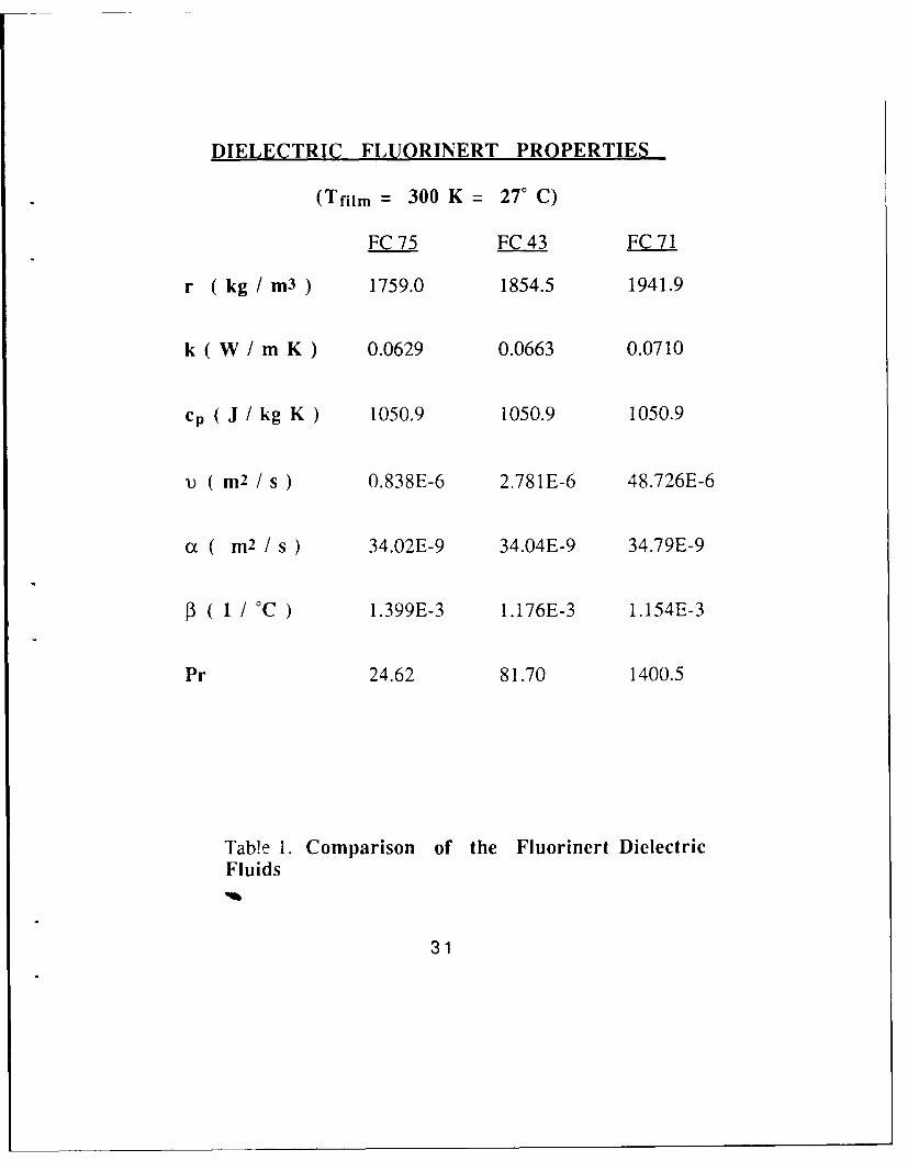
heat transfer characteristics of different dielectric fluids. The thermo-physical

properties of the fluids used are provided in Table 1. These values were determined

at a temperature of 300 K (Refer to Appendix A Sample Calculations for curve fit

equations used at other temperatures ). As seen in Table 1, the Prandtl number

varies from 24.2 for FC-75 to 1400.5 for FC-71.

Experiments were conducted using the Standard conditions of having the top

surface at 15 °C and the bottom at 10 °C.

For FC-75 (Figure 3.11 ) with a Prandtl number variation of approximately

30 to 25 in a range from 17 - 50 °C, the data indicate almost a single slope

except for the lowest power level (0. 1 W).

For FC-43 (Figure 3.12 ) with a Prandtl number variation of approximately

124 to 58 in a range 18 - 50 °C show similar trends. As for FC-75, the lowest

power level tends to deviate from the remaining data. As mentioned in the previous

section, this maybe due to the chamber boundary conditions which play an

important role at lower power levels. At higher power levels, the flow in the

vicinity of the component appears to dominate the heat transfer characteristics.

Also, in comparison to FC-75, for the same component power levels, the Rayleigh

numbers experienced a shift towards the left due to the higher fluid viscosities.

Additional experiments with FC-43 were performed with both boundaries

maintained at 15 C. The results (Figure 3.13 ) showed little deviation from the

30

DIELECTRIC FLUORINERT PROPERTIES

(Tfilm = 300 K = 270 C)

FC 75 FC 43 FC 71

r ( kg / m3 ) 1759.0 1854.5 1941.9

k ( W / m K) 0.0629 0.0663 0.0710

Cp ( J / kg K ) 1050.9 1050.9 1050.9

1) ( m2 / s ) 0.838E-6 2.781 E-6 48.726E-6

( m2 I s ) 34.02E-9 34.04E-9 34.79E-9

f3 (1 / °C ) 1.399E-3 1.176E-3 1.154E-3

Pr 24.62 81.70 1400.5

Tab!e 1. Comparison of the Fluorinert DielectricFluids

31

zu

C*

ZL

-C4

V)

w 0

jr) I pTrI H3waxlasa

32z

-~ L)

W~~~i N0 ntor OC

.4a

p-

Tam HdwamJ.,Issf0

z 33

L)

.0

~4.0

a0 4+ X 0 x

I3 J I I

34

CZ

t6

~a

35~

previous FC-43 case (Figure 3.12 ). This again demonstrates the effectiveness of

the temperature excess in correlating the heat transfer measurements for various

combinations of boundary temperatures.

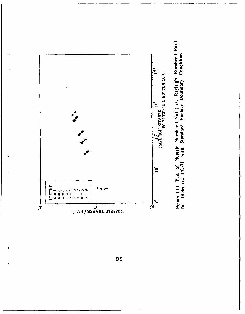
The final fluid was FC-71 (Figure 3.14 ) with a Prandtl number variation

of 2284 to 369 in the range 21 - 85 *C. Comparing these results with FC-75

shows a somewhat smaller slope of the variation. The large increase in fluid

viscosity shifts the Rayleigh number to the left by approximately 2 orders of

magnitude, at the same power levels.

a. Numerical Correlation of Data

The data for the various Prandtl number fluids for all power levels and

the standard boundary conditions were collected and presented in a Log - Log plot

of Nusselt (Nul ) and the flux based Rayleigh number (Figure 3.15 ). The

following best fit line was generated to determine the Nusselt number and Rayleigh

number relationship at a chamber width of 7 mm:

Nul = 0.29 Raf 0-2 168 (3.1)

where,

2* 106 < Raf < 1.5* 1010

15 < Pr < 2884

which is consistent with the results determined by Benedict [ Ref. 17] and Torres

[Ref. 18]. However, the differences in the geometry and enclosure dimensions in

these determinations should be emphasized.

36

Benedict [Ref. 17] used a horizontal orientation for the 3 by 3 protrusion

array. At a 120 mm by 144 mm by 30 mm chamber width using FC-75 dielectric

fluid it was determined that:

Nul = 0.28 Raf 0.22 (3.2)

where,

107 < Raf < 2 * 108

15 < Pr < 30.2

Torres [ Ref. 18] studied the 3 by 3 protrusion array in a vertical

configuration with the same chamber size as in the present experiment. The

dielectric fluid was FC-75 with the chamber width of 7 mm. The resulting best fit

equation was:

Nul = 0.073 Raf0.28 (3.3)

where,

3 * 108 < Raf < 1010

15 < Pr < 30.2

Both Benedict [ Ref. 17] and Torres [ Ref. 18] carried out measurements with the top

and bottom boundary temperatures of 10 *C.

Comparing equations 3.1, 3.2, and 3.3 reveals that moderate differences

in chamber width, changes in fluid Prandtl number, and protrusion orientation have

only a weak effect on the best fit equation. It must be emphasized, however, that

the best fit line does not corresponds to the lowest Nul values.

37

1.4-

zU

1.61

II

0.8

aa

U- 0

S1. 8

.-

Nul = 0.29 Raf 0.2168

38

Reviewing the data points that contributed to equation 3.1, shows the

greatest derivation from this fit corresponds to the lowest power level (0.1 W),

where the enclosure surface boundary conditions are the most significant. When

these points are not included in the curve fit, the resulting best fit line seen in

Figure 3.16 is given by:

Nul = 0.49 Raf0 .19 3 6 (3.4)

4. Selective Powering of Components

This was studied by energizing only one column of protrusions

(Components 4, 5, and 6 ) and in another set of experiments energizing

component 5 only. The standard surface conditions were employed with three

different dielectric fluids, in most experimental runs. Additional runs were made

with FC-75 with ambient (both the top and bottom at 19°C ) surface conditions.

The results (Figures 3.17 to 3.20) indicate higher Nusselt number values at

a given Rayleigh number, compared to fully powered array. This is expected since

the component temperature rise is smaller with partial powering of the array. The

highest Nusselt number resulted with the powering of only a single component.

With the single column energized, the lower the position of the component

within an column, the higher was the Nusselt number value at the same input

power. This is consistent with the numerical study conducted by Liu et. al.

Ref. 19].

39

1.8

U

1.6-

1.4-I

1.2-

1.0

0.8

6 7 8 9 10

Log RAYLEIGH NUMBER

Figure 3.16 Plot or Modified Best Fit Line, where,

Nul = 0.49 RarO.1936

40

+100+10 E0 0

E- u-4

am o u=4C

0 it

~ucl

-~ *~,L

'6z

- C2

0 c

-!PLM~f D OG.- U

1D1PT .01(mN ) H39flaN IlaSSflN

41

+ oil z .

E

z~

4.d~

P.O.

0042

m C

E

,oao

ol 0brA

o& E

z-~

UD Cc o

-A li 1 11 11 C0 0 4-+

'PI T .01 40mm) gawfm Ilssf-

43o

0~ C4

o E

43J

-40

oM

-p z

z z

Z 0 -4

'P tiI .0 TII

444-

B. FLOW VISUALIZATION

Flow visualization was conducted with the protrusion array oriented vertically

with the chamber width of 30 mm. The chamber width was chosen to allow

comparisons with the previous studies of Benedict j Ref. 17] and Torres [ Ref. 18].

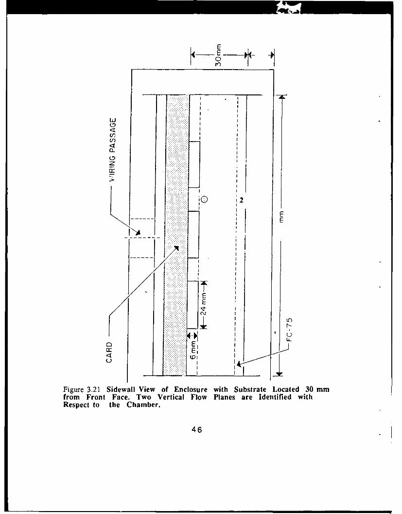
Visualizations were conducted in 3 vertical planes. As identified in Figure 3.21;

Plane 1 - aimed parallel towards the component through thesidewall

Plane 2 - aimed near and parallel to the front face of theenclosure through the sidewall

Plane 3 - Not shown in Figure 3.21, but was aimed perpendicularto the component and was viewed through the sidewall

A small amount of powered magnesium (325 Mesh ) was introduced into the

FC-75 Fluorinert dielectric fluid. These particles have a specific gravity of 1.92

gm/cm 3 and are almost neutrally buoyant in the Fluorinert fluids.

The top and bottom surfaces of the enclosure were maintained at uniform

temperatures close to the ambient levels. Visualizations were performed for input

power levels of 0.1, 0.7, and 1.5 W.

1. Flow Pattern with No Power Input

Visualization with no power was used to investigate the baseline Natural

Convection flow due to the temperature differences between the various chamber

surfaces. The flow in plane I (Figure 3.22 ) consisted of a dominant clockwise

flow, with both sidewall boundaries showing steady downward flow towards a

stable stratified region located at the base of the chamber.

Near the front face in plane 2 (Figure 3.23 ) circulating twin cells were

observed. Each cell had a dominant flow toward their respective sidewall and

down toward the stable stratified region at the chamber base.

45

E

UECD0

U) .I....... . . . . ... . .. .

<M

0. . . .. . .

. . . .. . ..........

* 7

EE

-~ C)

o E

Figure 3.21 Sidewall View of Enclosure with Substrate Located 30 mmfrom Front Face. Two Vertical Flow Planes are Identified withRespect to the Chamber.

46

06

z

0,0

00

w.C4

470

.E-

X

480

2. Flow Pattern at 0.1 W

With the heating of the components, a buoyant upflow was clearly evident

in plane 1 (Figure 3.24 ). Once the flow reached the top of the chamber it was re-

directed towards the sidewall boundaries and circulated back down into the stable

stratified region of colder dielectric fluid at the enclosure bottom.

In plane 2 (Figure 3.25 )the dual cell flow showed greater velocity along

the sidewall boundaries, toward the stagnan region at the bottom of the enclosure.

3. Flow Pattern at 0.7 W.

Observations adjacent to the components in plane 1 (Figure 3.26) showed

dominant upward flow only near the components. However small "eddies" were

observed near many components. Also observed was the strong downward flow

along the vertical sidewalls of the enclosure.

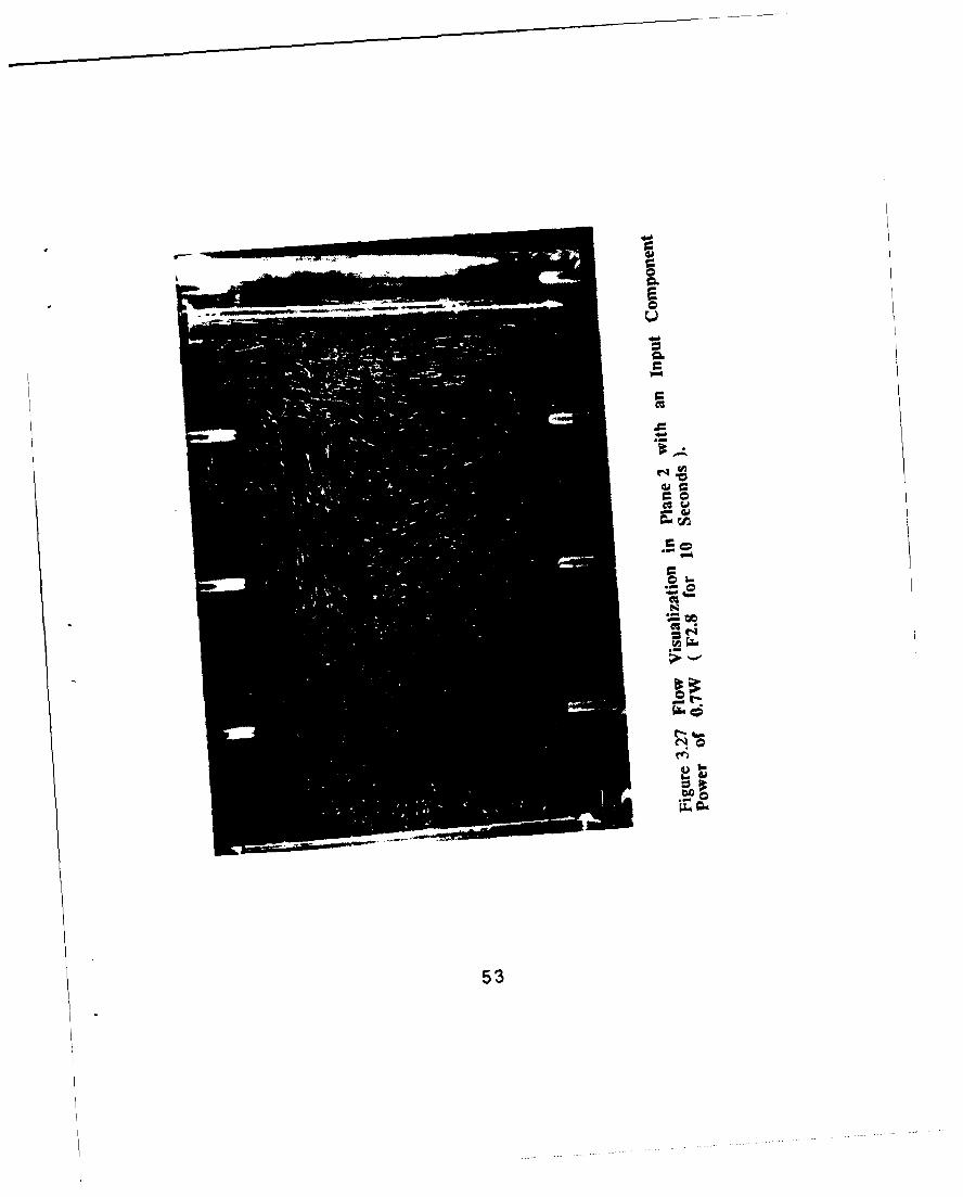
A strong clockwise circulation throughout the entire chamber was seen in

plane 2 (Figure 3.27 ). The sidewall boundary layers were found to be similar to

the previous power levels.

Looking at flow patterns in plane 3 (Figure 3.28 ), a 3 dimensional flow

structure was evident with an upflow near the components, an outward flow along

the enclosures' top boundary, and a downflow along the enclosure front face into

the colder stably stratified region near the bottom.

49

C00.E0Q

0.C

C

Co

.Su~C

I.-

C'.

ro

S~I~

50

06

2

06

51.

C

C0

20Q

C

=

=0'w~J

=OL

N

Sr-

u~.

52

06

b-40

53

Figure 3.28 Flow Visualization in Plane 3 with an Input Component

Power of 0.7W ( F2.8 for 15 Seconds ).

54

4. Flow Patterns at 1.5 W.

The flow observed at this power level appeared turbulent in nature. A

pronounced upflow near the component columns observed in plane 1 (Figure 3.29)

with formation of vortices at several locations. A dynamic downward flow along

the enclosure sidewalls toward the bottom region was also found, as for the lower

power levels.

In plane 2, upflow was also observed aligned with the component columns,

which was not seen at the lower power levels. As seen in Figure 3.30, the

presence of several small eddies were very evident. Observation of the 3

dimensional flow about plane 3 (Figures 3.31, 3.32, and 3.33 ), also indicates a

localized buoyant upflow region near the components.

55

C

CC

E0

C

C

- u~

Co

.EoCCi.

N

t~.

56

06

0

.5 c

N

57

Figure 3.31 Flow Visualization in Plane 3 with an Input Component

Power of 1.5W ( F2.8 for 10 Seconds ).

58

Figure 3.32 Close - Up Flow Visualization of Component 8 in Plane 3

with 1.5 W ( F2.8 for 10 Seconds ).

59

Figure 3.33 Close - Up Flow Visualization of Component 8 in plane 3

with 1.5 W ( F2.8 for 15 Seconds ).

60

IV. CONCLUSIONS

The thrust of this investigation was to increase the knowledge and data base

concerning single- phase, direct liquid cooling of a small array of discrete

protrusions. The data that was gathered established an understanding of the

phenomena present for a 3 by 3 protrusion array for,

A. Flow Visualization

Primarily upflow very near Components, downflow along the boundaries.

B. Heat transfer Measurements

1). Effects of Prandtl number can be correlated by suitable non-dimensional

parameters.

2). Enclosure Boundary Conditions relatively insignificant at higher power

levels.

3). Component Orientation relatively unimportant.

4). Chamber Width decrease marginally degrades heat transfer.

5). Selective Powering results in higher Nusselt number compared to fully

powered array at the same per component power.

61

V. RECOMMENDATIONS

1). Continuation of this investigation using other dielectic fluids with

superior thermophysical properties.

2). Conduct detailed Flow Visualization investigations at several chamber widths.

3). Develop comprehensive 3 Dimensional numerical models of flow and heat

transfer characteristics.

4). Manufacture a similar array with discrete flush heat sources, and conduct a

thorough investigation using the same parameters and compare results with this

study.

62

APPENDIX A SAMPLE CALCULATIONS

A. THERMOCOUPLE CONVERSION FROM VOLTAGES (emf)TO TEMPERATURES( - C)

HP 3497 Data Acquisition System (Channels 0 to 60 and 71 to 76)records given emf voltage readings in millivolts (mV) and convert totemperatures ( C). The coefficients are specifically for Omega CopperConstantan thermocouples.

T (°C) = 0.10086091 + (25727.9 * emf ) - (767345.8 * emf 2 ) +

(7802.5596 * emf 3 ) - ( 9247486589.6* emf 4 ) +

(6.98E II* emf 5 ) - (2.66E13*emf 6 ) + (3.94E14*emf 7 )

calculation: Using thermocouple 60 with FC-75 dielectric fluid at 1.5 Wattpower level yields,

emf = 0.000756 V = 0.756 mV

T = 20.70 *C

B. HEATER POWER (INPUT) CALCULATION

Hp 3497 Data Acquisition System ( Channels 62 to 70 ) are used tomeasure individual heater component voltages.

Qin (Watt) = (Vin - Vh) * Vh/ Rp

where

Vi, Supply Voltage (Channel 61)

Vh - Voltage across Heaters

Rp -Precision Resistor

63

calculation: The power dissipation of heater number 5 with dielectric fluid

FC-75 at 3.0 Watt power level was calculated to be

Qin = 5.314 * (6.717 - 5.314) / 2.50

Qi = 2.98 Watt

C. AVERAGE TEMPERATURE CALCULATIONS

1. Average Component Temperature

The facial temperatures of the fluid exposed faces were first multipliedby their respective Areas, and then summed together. This result was thendivided by the total fluid exposed Surface Area.

Tavg (*C) = Y' Ti * Ai / Atotal

= [ T (1) * Acen + T (2) * Atop + T (3) * Aright +

T (4) * Aleft + T (5) * Abot ] / Atotal

where

Acen - 0.024 * 0.008 = 1.92E-4 m 2

Aop =Abot = 0.006 * 0.008 = 4.85E-5 m 2

Aright Aleft= 0.006 * 0.024 = 1.44E-4 m 2

Atoa = I Ai = 5.76E-4 m 2

calculation: Using component 5 at the 3.0 W power level yields

Tavg (*C) = [(54.10 * 1.92E-4) + (54.93 * 4.8E-5) + (54.01 *

1.44E-4 ) + ( 54.42 * 1.44E-4 ) + ( 51.80 * 4.8E-5 )] / 5.76E-4

Tavg = 54.04 "C

64

2. Average Sink Temperature

Heat Exchanger Channels are averaged together.

Tsink (C)= Y [T top + Tbot ]/Number of Thermocouples

calculation: Using the 3.0 W power level

Tsink ('C) = [10.123 + 10.098 + 9.947 + 14.879 + 14.929] /5

Tsink = 11.99 "C

3. Average Film Temperature

Fluid film temperature is approximated as:

Tfilm (*C) = [ Tag + Tsink ] / 2

calculation: Using the previously determined values yields,

Tflm (*C) = [ 54.04 + 11.99 ] / 2

Tfilm = 33.02 °C

D. SUBSTRATE CONDUCTION LOSS CALCULATION

Q1oss(W)= AT/Rc

where

R,= L/k*A

= 0.0195m/(0.195W/mC)(0.008*0.024 M 2 )

= 520.83 °C/W

whereL- Plexiglass Substrate Thickness

k- Thermal Conductivity of Plexiglass

A- Back Area of Individual Component

65

calculation: Using the 3.0 W power level yields

Qloss (W) = [ 64.93 - 30.56 1 / 520.83

Qloss = 0.07 W

E. CONVECTION COEFFICIENT DETERMINATION

Recall, Newton's Law of Cooling

Qnet = Q - Qoss = h Atotal AT

Solving for h, yields

h (W / m2 C) =[Q - Qloss I / Atotal ( Tavg - Tsink )


h (W/ m2 C) = [ 3.0 - 0.07 ] / 5.76E-4 ( 54.04 - 11.99)

h = [ 2.93 ] / 5.76E-4 ( 42.05)

h = 120.97 W/m 2 C

F. FLUID PROPERTIES DETERMINATION

1. Thermal Conductivity k [ W / m *C I

From figure 5 of the 3M Corportation Flourinert ProductManual, the Thermal Conductivity coefficient curves have beendetermined to be:

FC - 75 0.065 - 7.89474E-5 * Tfilm

FC - 43 0.06660 - 9.864E-6 * Tfim

FC - 71 0.071

calculation: Using FC-75 with power level 3.0 W yields

kfluid ( W / m C) = 0.065 - ( 7.89474E-5 * 33.02)

knuid= 0.0624 W / m C

66

2. Density p [ Kg/rM3 ]

Using the expression on Table 4B and constants presented inTable 4C of the Product Manual yields;

FC - 75 (1.825 - 0.00246 * Tfim ) * 1000

FC - 43 (1.913 - 0.00218 * Tfiun ) * 1000

FC - 71 (2.002 - 0.00224 * Tntm ) * 1000

TfrIn temperatures must be in units of °C

calculation: Using FC-75 with the 3.0 W power level yields

p ( Kg / m 3 ) = [ 1.825 - ( 0.00246* 33.02)] * 1000

p = 1743.77 Kg/M 3

3. Kinematic Viscosity 1) [ m 2 / s ]

From figure 3 and determining a 4 th order curve fit yields:

FC - 75 [1.4074 - 2.96E-2 * Tfdm + 3.8018E-4 * Tfilm2

- 2.7308E-6 * Tfilm3 + 8.1679E-9 * TfiIm4 ] 1E-6

FC - 43 [8.8750 - 0.47007 * Tfin + 1.3870E-2 * TfiIm 2

- 2.1469E-4 * Tfilm3 + 1.3139E-6 * TfiIm4] 1E-6

FC - 71 [251.62 - 13.723 * Tfi + 0.30561 * Tfilm2

- 3.1704E-3 * Tfi] 3 + 1.2668E-5 * Tfilm4] 1E-6

67

calculation: Using FC-75 case with 3.0 W power level yields

U M2 / s ) = [1.4074 - 2.96E-2 ( 33.02 ) + 3.8018E-4 ( 33.02 )2

- 2.7308E-6 ( 33.02 )3 + 8.1679E-9 ( 33.02 )4 ] 1E-6

v 0.7546E-6 m2 / s

4. Specific Heat Cp [J / Kg *C I

For all Flourinert Electrochemicals (figure 4):

cp ( J / Kg *C)= ( 0.24111 + 3.70374E-4 *Tm )*4186


cp (J / Kg *C) = ( 0.2533) * 4186

Cp= 1060.5 J /Kg *C

5. Thermal Diffusivity a [ m 2 / s ]

Recalla = k/p cp


C( M2 / s ) = 0.0624/( 1743.77 * 1060.5)

a= 33.74E-9 m2 / s

6. Thermal Expansion Coefficient 13 [1 / °C I

Using expression in Table 4B and the constants presented inTable 4 C yields:

FC - 75 0.00246 / ( 1.825 - 0.00246 * Tijlm)

FC - 43 0.00218 / ( 1.913 - 0.00218 * Tflm)

FC - 71 0.00224 / ( 2.002 - 0.00224 * Tfl)

68

Tf-im temperatur,.'s must be in units of °C

calculation: Using FC-75 case with the 3.0 W power level yields

3( 1 / C ) = 0.00246/( 1.825 - 0.0812)

= 0.001411 / "C

G. CHARACTERISTIC LENGTHS

Two Characteristic Lengths have been formulated to enable comparisionswith other Experimental and Numerical Investigations.

LI Vertical length ( 0.024 m)

L2 Sum of the Ratios of Area to Perimeter of the Fluidexposed faces.

L2= X A(I)/P(I)= [(0.024 * 0.008) / 0.064 ] + 2 * [(0.008 * 0.006 ) I 0.028]+ 2 * [( 0.024* 0.006 ) / 0.060 ]

= [ 0.003 + 2 (0.00171429) + 2 (0.0024) ] m

L2 = 0.00112286 m

H. NUSSELT NUMBER DETERMINATION

Recall,

Nu = h L/k

each of the characteristic lengths defined above as used. Therefore,

Nul = h LI /kfluid

Nu2 = h L2 / knu id

calculation: Using FC-75 and the vertical length, Nul was determined

Nul = 120.97 * 0.024 / 0.0624

Nul = 46.53

69

I. GRASHOF NUMBER DETERMINATION

The Grashof Number indicates the ratio of Buoyancy force to theViscous force. Therefore,

Gr = g, ,L3*AT/U 2

where,g -Gravitational Constant


Gr = 9.81 * 0.001411 * (0.024)3 * 42.05/( 0.7546E-6 )2

Gr = 8.046E-6 / 5.694E-13

Gr = 14.13E+6

J. PRANDTL NUMBER DETERMINATION

Recall,

Pr-_o / ox

calculation: Using the Fc-75 case with the 3.0 W power level

Pr = 0.7546E-6 / 33.74E-9

Pr = 22.37

K. TEMPERATURE BASED RAYLEIGH NUMBER

DETERMINATION

Recall,

Rat- Gr * Pr

= g *P*L3*AT /1J*ox

70


Rat = 9.81 * 0.001411 * (0.024)3 * 42.05 / ( 0.7546E-6 * 33.74E-9)

Rat = 8.046E-6 / 25.46E-9 = 316.03E+6

L. FLUX BASED RAYLEIGH NUMBER

Recall,

Raf = g * * L4 * Qnet /k * a * ,u * Atot


Raf = [ 9.81 * 0.001411 * (0.024 )4 2.93 ] /

[ 0.0624 * 0.7546E-6 * 33.74E-9 * 5.76E-4 ]

Raf= 14.71E+9

71

APPENDIX B

UNCERTAINTY ANALYSIS

A. UNCERTAINTIES IN NET POWER ADDED INTO THE FLUID

Recall,

Qnet = Qn -Qloss

1. Qjn [Watt ]

Input Power is a function of the individual heater voltage, theinput voltage, and the precision resistors. Therefore,

DQim/aVh = Volt-2*Vh /RP

CQiC)Volt = Vh / RP

aQin/aRp =-Vh [VOlt-Vh ]/Rp

Thus,

UQin [( a Qin laVh) 2 * Uh2 +( a Qin /D Volt ) 2 * Uolt2 +

(aQin aRp)2 * URp2 ] 1/2

where,

Uvh = ± 0.001 Volt Resolution /Precision ot Measuring Device

Uvot= + 0.001 Volt

URp + 0.05 Q

72

calculation: Using FC-75 dielectric fluid with Chip 5 on the

3.0 W power level yields,

Vh = 5.314 V

Volt = 6.717 V

Rp = 2.50 Q

Therefore,

a Qm /a Vh =[6.717- (2*5.314)]/2.50=- 1.5644

aQin/ aVolt = 5.314/2.50 = 2.1256

a Qin/a Rp = [-5.314 • (6.717 - 5.314 )]/2.50 = -2.982

Thus

UQa' = [(1.5644)2 (0.001)2+(2.1256)2(0.001)2 +

(2.982)2(0.05)2 ]1/2

UQin = 0. 1491

Percentage error was derived by:

UQin / Qin = [0.1491 / 2.98 ], 100% = 5.00 %

Qin = 2.98 ± 5.0% Watt

Q101 [ Watt I

Recall,

Qloss= A T / Rc

73

The Energy loss due to conduction is a function of the change in

temperature, and the total thermal resistance. Therefore,

a Qlss /DAT = 1/R,

Qoss / Rc= AT/RC2

Thus,

UQoss = [(1 /R)2 * UT 2 +(AT/R2)2* URc2] 1/

where,

UAT = 10%

URc = 10%

calculation: Using FC-75 case with the 3.0 W power level yields

Rc= 520.97 * 10% = 52.097

AT = 64.93 - 30.56 = 34.37 *C

Therefore,

Qioss / a Rc= 1 / 520.97 = 0.001919

) Qlos / a AT = 34.37 / (520.97)2 = 126.64E-6

Thus,

UQIoss ((0.001919)2 (3.437)2 +(126.64E-6)2 (52.097;7 ]1/2

UQioss = 0.00933

Pecentage error was derived by:

UQioss I Qjoss = 0.00933 /0.07 * 100% = 13.3%

= 0.07 ± 13.3% Watt

74

3. Qnet [Watt ]

Combining the results of the power and energy lossuncertainties yields the final uncertainty calculation for Qet:

UQnet = [(UQin ) 2 + ( UQIoss ) 2 ] 1/2

calculation: Using FC-75 with the 3.0 W power level yields,

UQnet = [(0.1491)2 + (0.00933)2 ] 1/2

UQnet = 0.1494

Percentage error was dervived by:

UQnet/Qnet = [0.1494/2.93] * 100% = 5.10%

0 = 2.93 ± 5.1% Watt

B. UNCERTAINTY IN NUSSELT NUMBER

Recall,

Qnet = h Atotal ( Tavg- Tsink )

Solving for the Heat Transfer coefficient, h, yields,

h = Q / Atotal ( Tavg - Tsink )

where the Heat Transfer coefficient is a function of the net power dissipatedby the heater, total area, and the change in temperature. Therefore,

h/aQnet= 1/AtotlAT

ah / Attato = Qnet /Aotal AT

ah/c(AT) =Qet/Atotal (AT)2

Thus,

U =h h / Qne ) 2 * UQnet 2 + (h / AtotaI ) 2 * UAtota 1

+ (ah/aAT)2*UAT2 1/2

75

where,

UAtotal = [(aAtotal/aL)2 * UL2 +(DAtotai/aW) 2 * UW2 + (Atotal/DH)2 * UH2 ] 1/2

= [ (2H + W )2 (1E-4)2 + 2 (L + W )2 (1E-4)2 +

( 2H + L )2 (1E-4)2 ]1/2

UL = IE-4m

UAtota = 8.736E-6 m2

UAT = + 1%

calculation: Using Fc-75 at the 3.0 W power level yields,

AT = 54.04 - 11.99 = 42.05 °C

Atom, = 5.76 E-4 m2

Therefore,

a h /a Qet = I / [(42.05)(5.76E-4) ] = 41.29

a h / Atom = 2.93 Lt (42.05)(5.76E-4) ] = 120.97

a h / a(AT) = 2.93 / [(5.76E-4)(42.05)2] = 2.877

Thus,

Uh =[(41.29)2 (0.1494)2 +(120.97)2 (8.736E-6)2 +

(2.877)2 (0.4205)2] 1/2

Uh = 6.286


Uh/h = [ 6.286/120.971 * 100% = 5.20 %

h= 120.97 ± 5.2%

76

Recall, to determine the Nusselt Number

Nu = hL/k

The Nusselt Number is a function of the Heat Transfer Coefficient,Characteristic length, and the Thermal Conductivity. Therefore,

DNu/)h = L/kfhid

D Nu/c aL = h /kfluid

DNu/Dk = -hL/kfluid 2

Thus,

UNu= I (DNu/ h )2* Uh2 + (. Nu/ a L )2 * UL2 ] 1/2

Assuming that the Dielectric Flourinert Fluids' properties are

considered to have no uncertainty in this determination.

calculation: Using FC-75 with the 3.0 W power level yields,

a Nul / ah = 0.024 / 0.0624 = 0.3846

aNul/aL = 120.97/0.0624 = 1938.6

Thus,

UNul = [(0.3846)2 (6.286)2 +(1938.6)2 (1E-4)2] 1/2

UNul = 2.425


UNul / Nu [2.425 / 46.53 1 * 100% = 5.2 %

Nul = 46.53 ± 5.2 %

77

C. FLUX BASED RAYLEIGH NUMBER DETERMINATION

Recall the expression for the Rayleigh Number,

Raf = Grf Pr

where,

Grf= g 3 L4 Qnet / kf '12 Ato

Pr = u/oa

The Grashof number is a function of gravity (g), volumetric expansioncoefficient ( f3 ), characteristic length ( L), net power dissipated ( Qnet ), thermal

conductivity (k ), kinematic viscosity (i), and total wetted area (Atotal).Therefore,

UGrf /Grf = [(DQne t / Qnet) 2 +(4) L/ L) 2 +(DAtotal/ Attal) 2] 1/2

calculation: Using FC-75 at the 3.0 W power level yields

UGr/Grf =[(0.1494/2.93) 2 +(4E-4/0.024) 2 +(8.736E-6/5.76E-4)] 1/2


UGrf/Grf = URaf/Raf = 0.0558 * 100% = 5.58 %

Ra-f = 14.71 E+9 ± 5.58 %

78

APPENDIX C

The following graphical representations are for the sake of brevity to show the

Heat Transfer measurements per component that was gathered during this

investigation.

79

OOTZ O O~ - r..+ ~~ -0 ifU- .:

0x -0 .4 +t x C>

E-~Z

-4o

80L.

DL- -UU- - --- :

LL. zdi Ii I I I I I I I

x0

+C11

..> Eez z

r4

-OPEI.

Z=

uz

PT PoTflKH~g~im 13SR-

81e

" N-UU-UU- -t

CZ. ".". C6

0 4 4 C>48

x=

x WD4~3

r~z

6

cc

gp pIfIN ggwammassa

82~

o o00"000

X u )L)UU U3

x 0 4+x0C ax40 E

-z 6

-QO

I-I-

(inN H~gwflN L,13ssflN

83

- Ir)t C L

+

0 0D x 0-~ Q Q Q 0o-

0~ 0

0-u

-4

~~OI

an InN H3NfN ITOlel

84

z CD*~ L .. L -4

711c LoU-

zZ

zz

o

-Q

00

ici

I-

85

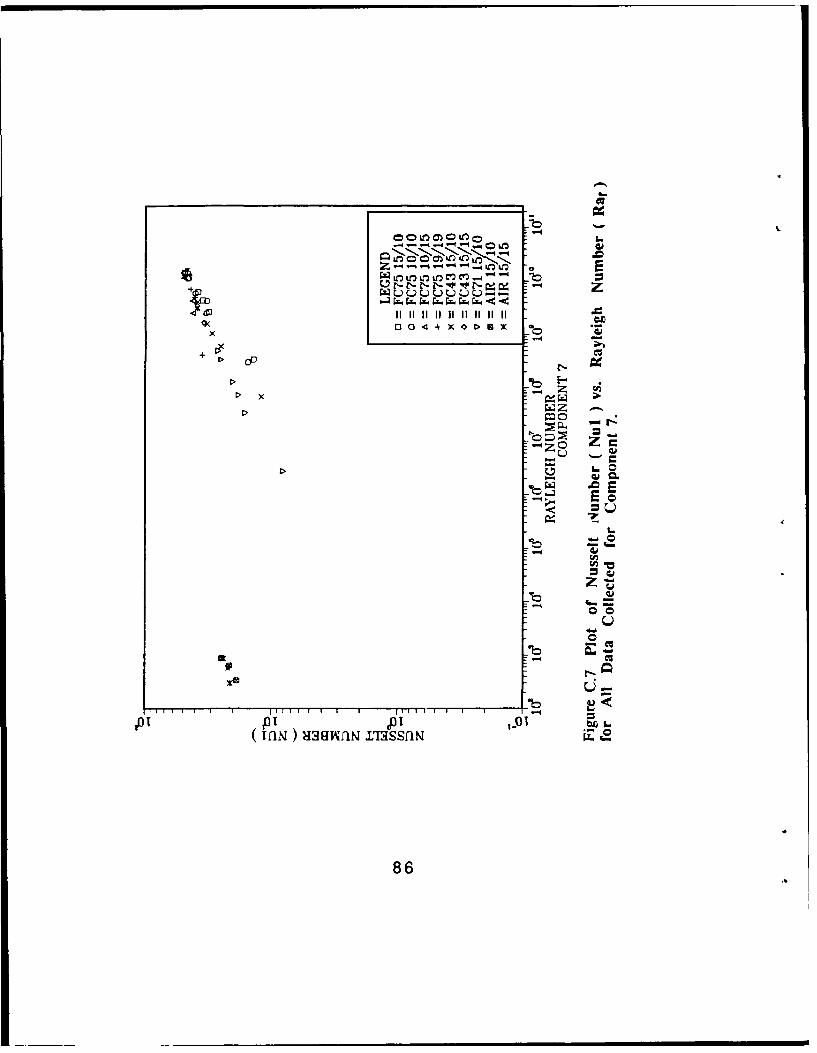
II --I II I -II II I I

+ CIS

X~

z

I I I i i II I I I 1 11I1 t 1 1 1 I I I I I II I

u ,

'01 pi,01,Oi ,

86

" -.4 -.4 O

0 m - -~ '

-

*x 0 4 x C x

x

~o c

12

OAR ZcLi'-

JTT T I I Fj i I I I

.. .....-

z - 4 - -4 " - I) t

r-- f- r 42

co It 11 11 11 It 11 II1I

+

zu

z I.-

-b00

2

(im ) gRwflN £I3SSflN

88

LIST OF REFERENCES

1. Oktay, S., "High Heat from Small Package," Mechanical Engineering,Vol. 108, pp 36-42, March, 1986.

2. Chu, R., "Heat Transfer in Electronic Systems," Proc. of the 8 thInternational Heat Transfer Conference, San Francisco, California, pp293-305, 1986.

3. Incropera, F., " Convection Heat Transfer in Electronic EquipmentCooling," Journal of Heat Transfer, Vol. 110, pp 1097-1111, November,1988.

4. Hannemann, R., Incropera, F.P., Simons, R., " Research Needs inElectronic Cooling ," Proc. of a National Science Foundation / PurdueUniversity Workshop, Edited by F.P. Incropera, December, 1986.

5. Baker, E., " Liquid Cooling of Microelectronic Devices by Free and ForcedConvection ," Microelectronics and Reliability, Vol. 11, pp 213-222,April, 1973.

6. Baker, E., "Liquid immersion Cooling of Small Electronic Devices,"Microelectronics and Reliability, Vol. 12, pp 163-173, 1973.

7. Park, K.A. and Bergles, A.E., " Natural Convection Heat TransferCharacteristics of Simulated Microelectronic Chips," Transactions ofASME, Journal of Heat Transfer, Vol. 109, pp 90-96, February,1987.

8. Keyhani, M., Prasad, V., and Cox, R., " An Experimental Study of NaturalConvection in a Vertical Cavity with Discrete Heat Sources," ASMEPaper No. 87-HT-76, 1987.

9. Chen, I., Keyhani, M., and Pitts, D.R., "An Experimental Study of NaturalConvection Heat Transfer in a Rectangular Enclosure with ProtrudingHeaters ," Paper presented at National Heat Transfer Conference,Houston, Texas, 1988.

10. Liu, K.V., Kelleher, M.D., and Yang, K.T., "Three Dimensional NaturalConvection Cooling of an Array of Heated Protrusions in an EnclosureFilled with a Dielectric Fluid," Proc. Int. Symposium on CoolingTechniques for Electronic Equipment, Honolulu, Hawaii, March, 1987.

89

11. Kelleher, M.D., Knock, R.H., and Yang, K.T., " Laminar NaturalConvection in Rectangular Enclosure Due to a Heated Protrusion on OneVertical Wall - Part 1: Experimental Investigation", Proc. 2nd ASME / JSMEThermal Engineering Joint Conference , Honolulu, Hawaii, pp 169-177,1987.

12. Lee, K.V., Kelleher, M.D., and Yang, K.T., " Laminar Natural Convectionin a Rectangular Enclosure Due to a Heated Protrusion on One VerticalWall - Part II: Numerical Simulations ", Proc. 2 nd ASME / JSME ThermalEngineering Joint Conference , Honolulu, Hawaii, pp 179-185, 1987.

13. Joshi, Y., Kelleher, M.D., and Benedict, T. J., " Natural ConvectionImmersion Cooling of an Array of Simulated Electronic Components inan Enclosure Filled with Dielectric Fluid ", Proc. of the InternationalSymposium on Heat Transfer in Electronic and Microelectronic EquipmentDubrovnik, Yugoslavia, 1988.

14. Knock, R.H., "Flow Visualization Study of Natural Convection from aHeated Protrusion in a Liquid Enclosure ", Master of Science Thesis,Naval Postgraduate School, Monterey, California, December, 1983.

15. Hazard, S.J., " Single Phase Liquid Immersion Cooling of Discrete HeatSources on a Vertical Channel ", Master of Science Thesis, NavalPostgraduate School, Monterey, California, December, 1986.

16. Pamuk, T., " Natural Convection Immersion Cooling of an Array ofSimulated Components in an Enclosure Filled with Discrete Fluid ",

Master of Science Thesis, Naval Postgraduate School, Monterey,California, December, 1987.

17. Benedict, T.J., "An Advanced Study of Natural ConvectionImmersion Cooling of a 3 X 3 Array of Simulated Components in anEnclosure Filled with Dielectric Liquid ", Master of Science Thesis, NavalPostgraduate School, June, 1988.

18. Torres, E., " Natural Convection Cooling of a 3 by 3 Array ofRectangular Protrusions in an Enclosure Filled with Dielectric Liquid:Effects of Boundary Conditions and Component Orientation, Master ofScience Thesis, Naval Postgraduate School, December, 1988.

19. Liu, K.V., Yang, K.T., Wu, Y.W. and Kelleher, M.D., " Local OscillatorySurface Temperature Responses in Immersion Cooling of a Chip Arrayby Natural Convection in an Enclosure ", Proc. of the Symposium onHeat and Mass Transfer in Honor of B. T. Chao , University ofIllinois, Urbana - Champaign, pp 309-330, October, 1987.

90

INITIAL DISTRIBUTION LIST

No. Copies

I. Defense Technical Information Center 2Cameron StationAlexandria, VA 22304-6145

2. Library, Code 0142 2Naval Postgraduate SchoolMonterey CA 93943-5002

3. Professor Y. Joshi, Code 69J1 2Department of Mechanical EngineeringNaval Postgraduate SchoolMonterey CA 93943-5004

4. Professor M.D. Kelleher, Code 69KkDepartment of Mechanical EngineeringNaval Postgraduate SchoolMonterey CA 93943-5004

5. Department Chairman, Code 69Department of Mechanical EngineeringNaval Postgraduate SchoolMonterey CA 93943-5004

6. Mr. Duane EmbreeNaval Weapons Support CenterCode 6042Crane, IN 47522

7. Mr. Alan BoslerNaval Weapons Support CenterCode 6042Crane, IN 47522

8. Mr. Joseph CiprianoExecutive DirectorWeapons and Combat Systems DirectorateNaval Sea Systems CommandWashington D.C. 20362-5101

91

9. Naval Engineering Curricular Officer, Code 34 1Department of Mechanical EngineeringNaval Postgraduate SchoolMonterey CA 93943-5004

10. Professor H. Julien 1Department of Mechanical EngineeringBox 3001 Dept. 3450New Mexico State UniversityLas Cruces NM 88003

11. Lt. Mark E. Powell USN 2P.O. Box 216Omena MI 49674

92

ic copy naval postgraduate school monterey, california=onvection immersion cooling of a three by...

Documents