ic2it 2013 presentation

Dhaka Stock Exchange Trend Analysis Using Support

Vector Regression

Authors:Phayung Meesad & Risul Islam Rasel

Faculty of Information Technology

King Mongkut’s University of Technology North Bangkok

Email: [email protected]; [email protected]

The 9th International Conference on Computing and Information Technology (IC2IT 2013)

KMUTNB

9th May 20113 IC2IT 2013 2

Outline

�Introduction

�Related work

�Motivation & Goal

�Experiment design

�Result analysis

�Conclusion

9th May 20113 IC2IT 2013 3

1. Introduction

• Stock exchange :

� is an emerging business sector has become more popular among the people.

� many people, organizations are related to this business.

� gaining insight about the market trend has become an important factor

• Stock trend or price prediction is regarding as challenging task because

� Essentially a non-liner, non parametric

� Noisy

� Deterministically chaotic system

• Why deterministically chaotic system?

� Liquid money and Stock adequacy

� Human behavior and News related to the stock market

� Share Gambling

� Money exchange rate, etc.

9th May 20113 IC2IT 2013 4

2. Related Work

2.1 Support Vector regression (SVR)

• Support vector machine (SVM), a novel artificial intelligence-based method

developed from statistical learning theory

• SVM has two major futures: classification (SVC) & regression (SVR).

• In SVM regression, the input is first mapped onto a m-dimensional feature space

using some fixed (nonlinear) mapping, and then a linear model is constructed in this

feature space.

• a margin of tolerance (epsilon) is set in approximation.

• This type of function is often called – epsilon intensive – loss function.

• Usage of slack variables to overcome noise in the data and non - separability

9th May 20113 IC2IT 2013 5

Related Work (cont..)

• Support vector regression (SVR) model with parameters w and b can be expressed as

• where y is the model output and input x is mapped into a feature space by a nonlinear function (x).

f(x) = w.z (x) + b

Image courtesy: Pao-Shan Yu*, Shien-Tsung Chen and I-Fan Chang

9th May 20113 IC2IT 2013 6


• The regression problem of SVM can be expressed as the following optimization

problem.

w,b,p,p*

min

21 | | w | | 2 + c (p + p*)

i=1

l/

subject to yi - (w.z (xi) + b) # f + p

(w.z (xi) + b) - yi # f + p*

p ,p*$ 0, i = 1, 2, ......, l

p• Where and are slack variables that specify the upper and the lower training errors

subject to an error tolerance ε.

• C is a positive constant that determines the degree of penalized loss when a training

error occurs

p*

9th May 20113 IC2IT 2013 7


2.2 Windowing operator

• The problem of forecasting the class attribute x, N steps ahead of time, as learning a

target function which uses a fixed number of M past values.

x(t+N) = f([x(t-0), x(t-1), …, x(t-M)]) ……………(1)

• This equation can be written as:

x-0 = f([x-0, x-1, ..., x-M] – [x-0, x-1, …, x-N])

or as: x-0= f([x-0, x-N, ..., x-M]) …………………(2)

or in the multivariate case as:

x-0 = f([x-0, y-0, x-1, y-1 ..., x-M, y-M] – [x-0, x-1, y-1, …, x-N, y-N]) …. (3)

• Since Windowed Examples are of the form: [x-0, x-N, y-N, ..., x-M, y-M], we have

to remove all horizon attributes: [x-1, y-1, …, x-N, y-N].

• The result is a dataset with Windowed Examples which can be fed to any machine

learning algorithm.

9th May 20113 IC2IT 2013 8

Notations:•0 timestep 0,the timestep we wish to predict.

•N the number of timesteps between now and

0

•M the size of the window

•attribute-[0-9] a Windowed Attribute,

measured at timestep [0-9]

•x-0 attribute x measured at timestep 0

•x-0 equivalent to x-0

•x(t+N) equivalent to x(0), if t+N is the

timestep we wish to predict

9th May 20113 IC2IT 2013 9


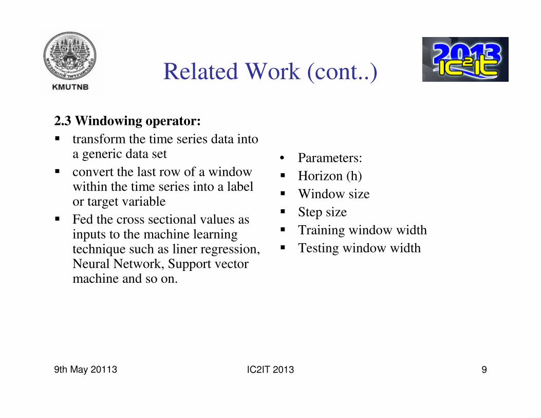
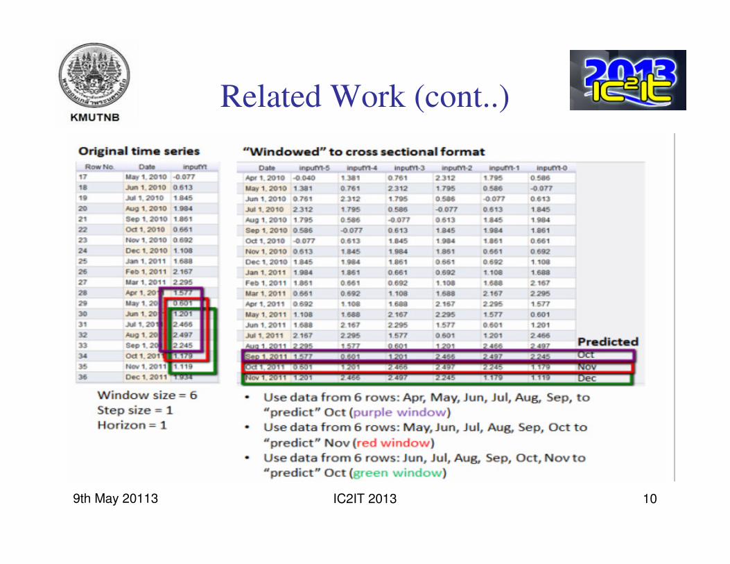
2.3 Windowing operator:

� transform the time series data into a generic data set

� convert the last row of a window within the time series into a label or target variable

� Fed the cross sectional values as inputs to the machine learning technique such as liner regression, Neural Network, Support vector machine and so on.

• Parameters:

� Horizon (h)

� Window size

� Step size

� Training window width

� Testing window width

9th May 20113 IC2IT 2013 10


9th May 20113 IC2IT 2013 11


2.4 Some recent research works

1. “Stock Forecasting Using Support Vector Machine,”• Authors: Lucas, K. C. Lai, James, N. K. Liu

• Applied technique: SVM and NN

• Data preprocess technique: Exponential Moving Average (EMA15) and relative difference in percentage of price (RDP)

• Domain: Hong Kong Stock Exchange

2. “Stock Index Prediction: A Comparison of MARS, BPN and SVR in an Emerging Market,”

• Authors: Lu, Chi-Jie, Chang, Chih-Hsiang, Chen, Chien-Yu, Chiu, Chih-Chou, Lee, Tian-Shyug,

• Applied technique: Multivariate adaptive regression splines (MARS), Back propagation neural network (BPN), support vector regression (SVR), and multiple linear regression (MLR).

• Domain: Shanghai B-share stock index

9th May 20113 IC2IT 2013 12


• So, many research have been done using support vector machine (SVM) in

order predict stock market trend.

• GA, EMA, RDP and some other techniques have been used as input

selection technique or optimization technique. So, Still there are some

scope to apply different input selection or optimization technique to fed

input to the machine learning algorithm like support vector machine and

Neural network.

3. “An Improved Support Vector Regression Modeling for Taiwan Stock

Exchange Market Weighted Index Forecasting,”

• Authors: Kuan-Yu. Chen, Chia-Hui. Ho

• Applied technique: SVR, GA, Auto regression (AR)

• Domain: Taiwan Stock Exchange

9th May 20113 IC2IT 2013 13

3. Motivation & Goal

• Motivation:

� SVR is a powerful machine learning technique for pattern recognition

� Introducing of using different kinds of windowing function as data preprocess is a

new idea

� Combining windowing function and support vector regression can make good

model for time series prediction.

• Goal:

� Propose a good Win-SVR model to predict stock price

9th May 20113 IC2IT 2013 14

4. Experiment Design

4.1 Data collection� Experiment dataset had been collected from Dhaka stock exchange (DSE),

Bangladesh.

� 4 year’s (January 2009-June 2012)historical data were collected.

� Almost 522 company are listed in DSE. But for the convenient of the experiment we only select one well known company data.

� Dataset had 6 attributes. Date, open price, high price, low price, close price, volumes.

� 5 attributes were used in experiment except volumes.

� Total 822 days data. 700 data were used as training dataset, and 122 data were used as testing dataset.

9th May 20113 IC2IT 2013 15

Experiment Design (cont..)

Training phase

• Step 1: Read the training dataset from local repository.

• Step 2: Apply windowing operator to transform the time series data into a generic dataset. This step will convert the last row of a window within the time series into a label or target variable. Last variable is treated as label.

• Step 3: Accomplish a cross validation process of the produced label from windowing operator in order to feed them as inputs into SVR model.

• Step 4: Select kernel types and select special parameters of SVR (C, ε , g etc).

• Step 5: Run the model and observe the performance (accuracy).

• Step 6: If performance accuracy is good than go to step 6, otherwise go to step 4.

• Step 7: Exit from the training phase & apply trained model to the testing dataset.

Testing phase

• Step 1: Read the testing dataset from local repository.

• Step 2: Apply the training model to test the out of sample dataset for price prediction.

• Step 3: Produce the predicted trends and stock price

4.2 Model Work Flow

9th May 20113 IC2IT 2013 16


4.3 Optimal Window settings

• Three types of Windowing operator were used as data preprocess.

� Normal rectangular window

� Flatten window

� De- flatten window

• Optimal settings of windowing components for SVR models are given below:

303015AllDe-Flatten window

303012522 days

3030185 days

3030131 day

Flatten window

303013AllRectangular

Test

window

width

Training

window

width

Step

size

Window

sizeModel

Windowing

operator

Table 1: Window settings

9th May 20113 IC2IT 2013 17


4.4 SVR kernel Parameters settings• Model 1: 1 day a-head prediction model

• Model 2: 5 days a-head prediction model

• Model 3: 22 days a-head prediction model

• Kernel function: Radial basis function (RBF)

112110000RBFModel-3

112110000RBFModel-2

112110000RBFModel-1

ε-ε+εgCKernelSVR Model

Table 2: SVR kernel parameters setting

9th May 20113 IC2IT 2013 18


4.5 Proposed Win-SVR Models� 1 day & 5 days a-head model

• Window type: Flatten Window

• Window size : 3 (1 day model), 8 (5 days model)

• Attribute selection : All

• Step size : 1

• T.W.W : 30, t.s.w : 30, Kernel type : RBF

2187.6622762.022219.7272587.202

w[Close-6]w[Close-7]w[Low-6]w[Low-7]

2447.792231.121716.6161792.63-4.658687

w[High-6]w[High-7]w[open-6]w[open-7]

5 days

-546.558-1087.763-1074.989-746.5163.335696

w[Close-2]w[Low-2]w[High-2]w[open-2]

1 day

Weight (w)Bias (b)SVModel

Table 3: SVR model for Flatten window

9th May 20113 IC2IT 2013 19


� 22 days a-head model

• Window type: Normal Rectangular window

• Window size : 3

• Attribute selection : single attribute (close)

• Step size : 1

• T.W.W : 30, t.s.w : 30, Kernel type : RBF

805.11631.51719.6421.367522 days

w [close-0]w [close-1]w [close-2]b SV

Weight (w)Bias

(offset)

Support

Vector Model

Table 4: SVR model for normal rectangular window

9th May 20113 IC2IT 2013 20

5. Result Analysis

Result evolution technique:

� Error calculation: Used MAPE

� MAPE: Mean Average Percentage Error (MAPE) was used to calculate the error rate

between actual and predicted price.

MAPE = 100n

|A

A - P |i = 1

n

/Here,

A = Actual price

P = Predicted price

n = number of data to be counted

9th May 20113 IC2IT 2013 21

Result Analysis (cont..)

Actual vs Predicted price

1 day a-head model

0

50

100

150

200

250

300

1 8 15 22 29 36 43 50 57 64 71 78 85 92 99 106 113 120

Days (Jan-Jun'2012)

Clo

se P

rice (

BD

T)

Actual Predicted

Actual vs Predicted close price

22 days a-head model

0

50

100

150

200

250

300

1 6 11 16 21 26 31 36 41 46 51 56 61 66 71 76 81 86 91 96

Days (Jan-May'2012)

Clo

se P

rice (

BD

T)

Actual Predicted

Actual vs Predicted price

5 days a-head model

0

50

100

150

200

250

300

1 7 13 19 25 31 37 43 49 55 61 67 73 79 85 91 97 103 109

Days (Jan-jun'2012)

Clo

se

pri

ce

(B

DT

)

Actual Predicted

•Fig 1: 1 day a-head model result from flatten

window (MAPE : 0.04 )

•Fig 2: 5 days a-head model result from flatten

window (MAPE : 0.15 )

•Fig 3: 22 days a-head model result from

rectangular window (MAPE : 0.22 )

Fig:1 Fig:2

Fig:3

9th May 20113 IC2IT 2013 22

Result Analysis (cont..)

Error rateDe-flatten window

0

2

4

6

8

10

12

14

16

Jan Feb Mar Apr May

Months

MA

PE

1 day a-head 5 days a-head 22 days a-head

Error rateNormal Rectangular window

0

0.5

1

1.5

Jan Feb Mar Apr May

Month

MA

PE


Error rateFlatten window

0.00

0.10

0.20

0.30

0.40

0.50

Jan Feb Mar Apr May

Month

MA

PE


7.610.220.2222

22 days a-

head

7.160.150.2655 days a-head

7.790.040.4211 Day a-head

De-

flatten

window

Flatten

window

Rectangul

ar windowHorizonModel

Table :Average MAPE (error) for test data (From Jan’12 to May’12)

Fig:4 Fig:5

Fig:6

9th May 20113 IC2IT 2013 23

6. Conclusion

6.1 Discussions :

� Different windowing function can produce different prediction results.

� We used 3 types of windowing operators. Normal rectangular window, Flatten

window, De-flatten window.

� Rectangular and flatten windows are able to produce good prediction result for time

series data.

� De-flatten window can not produce good prediction results.

6.2 Limitations & Future works:

� Here we only use 3 types of windowing operators.

� Only one stock exchange data set were used to undertake the experiments.

� Do not compare with other machine learning techniques.

� In future, we will apply our model to other stock market data set and will also

compare our research result with other types of data mining techniques.

9th May 20113 IC2IT 2013 24

THANK YOU

FOR YOUR ATTENTION

The 9th International Conference on Computing and Information Technology (IC2IT 2013)

KMUTNB