icaps 2014icaps14.icaps-conference.org/proceedings/keps/keps_proceedings.pdfable set vs refers to...

Proceedings of the 5th Workshop on Knowledge Engineering for Planning and Scheduling

Edited By:

Roman Barták, Simone Fratini, Lee McCluskey and Tiago Vaquero

Portsmouth, New Hampshire, USA -‐ June 22, 2014

ICAPS 2014

Organizing Committee Roman Barták Charles University, Czech Republic Simone Fratini European Space Agency, Germany Lee McCluskey University of Huddersfield, UK Tiago Vaquero University of Toronto, Canada

Program Committee Roman Barták, Charles University, Czech Republic Daniel Borrajo, Universidad Carlos III de Madrid, Spain Adi Botea, IBM, Ireland Amedeo Cesta, ISTC-‐CNR, Italy Susana Fernández, Universidad Carlos III de Madrid, Spain Simone Fratini, European Space Agency, Germany Antonio Garrido, Universidad Politecnica de Valencia, Spain Arturo González-‐Ferrer, Universidad Carlos III de Madrid, Spain Felix Ingrand, LAAS-‐CNRS, France Lee McCluskey, University of Huddersfield, UK Ugur Kuter, SIFT, USA Julie Porteous, Teesside University, UK Kanna Rajan, MBARI, USA José Reinaldo Silva, University of São Paulo, Brazil Tiago Vaquero, University of Toronto, Canada Dimitris Vrakas, Aristotle University of Thessaloniki, Greece Gerhard Wickler, University of Edinburgh, Scotland

Foreword The KEPS 2014 workshop aims to promote research in the areas lying between planning & scheduling technology on the one side, and practical applications and problems on the other. Despite recent advances in the area, the performance of planning & scheduling systems is still dependent to a large extent on how problems and domains are formulated, resulting in the need for careful system fine-‐tuning. In particular, recent work with competition benchmark problems highlights the importance of the relation between how domain knowledge is engineered within a model, and the efficiency of planning engines when input with these models. Knowledge engineering for planning & scheduling covers a wide area, including the acquisition, formalization, design, validation and maintenance of domain models, and the selection and optimization of appropriate planning engines to work on them. Knowledge engineering processes impact directly on the success of real planning and scheduling applications. The importance of knowledge engineering techniques is clearly demonstrated by a performance gap between domain-‐independent planners and planners exploiting domain dependent knowledge. This year the set of accepted papers reproduced in these proceedings reflects the wide scope of knowledge engineering within the ICAPS area. There are papers on techniques in engineering real applications, such as in clinical rehabilitation, and in hypothesis generation in medical and network domains. Two papers consider plans -‐ one to develop the means for estimating upper bounds of plan length from planning problems, and the other in optimizing solution plans by removing redundant actions within them. Problem transformation is an area which is growing in importance, and in these proceedings we have two papers on this issue, one looking at ways of decomposing very complex planning problems to expedite solutions, and another to compile problems with soft constraints into a form usable by mainstream planning engines. Finally, we have contributions on knowledge capture -‐ one a review of automated domain model acquisition, and the other describing a new knowledge-‐based language designed to enable subject-‐matter experts to formulate knowledge in planning applications. Roman Barták, Simone Fratini, Lee McCluskey, Tiago Vaquero KEPS 2014 Organizers June 2014

Table of Contents Mechanising Theoretical Upper Bounds in Planning ................................................. 1 Mohammad Abdulaziz, Charles Gretton, Michael Norrish Applying Problem Decomposition to Extremely Large Planning Domains ................. 8 Masataro Asai, Alex Fukunaga Eliminating All Redundant Actions from Plans Using SAT and MaxSAT ................... 16 Tomáš Balyo, Lukáš Chrpa Planning with Preferences by Compiling Soft Always Goals into STRIPS with Action Costs ......................................................................................................................... 23 Luca Ceriani, Alfonso Emilio Gerevini Automated Knowledge Engineering Tools in Planning: State-‐of-‐the-‐art and Future Challenges ................................................................................................................ 31 Rabia Jilani, Andrew Crampton, Diane Kitchin, Mauro Vallati Goal-‐directed Generation of Exercise Sets for Upper-‐Limb Rehabilitation .............. 38 José C. Pulido, José C. González, Arturo González-‐Ferrer, Javier García, Fernando Fernández, Antonio Bandera, Pablo Bustos, Cristina Suárez Knowledge Engineering for Planning-‐Based Hypothesis Generation ....................... 46 Shirin Sohrabi, Octavian Udrea, Anton V. Riabov Creating Planning Domain Models in KEWI ............................................................. 54 Gerhard Wickler, Lukáš Chrpa , Thomas Leo McCluskey

Mechanising Theoretical Upper Bounds in Planning

Mohammad Abdulaziz and Charles Gretton and Michael Norrish ∗

Canberra Research Lab., NICTA7 London Circuit, Canberra ACT 2601, Australia

{Mohammad.Abdulaziz, Charles.Gretton, Michael.Norrish}@nicta.com.au

Abstract

We examine the problem of computing upper bounds onthe lengths of plans. Tractable approaches to calculat-ing such bounds are based on a decomposition of state-variable dependency graphs (causal graphs). Our contri-bution follows an existing formalisation of concepts inthat setting, reporting our efforts to mechanise bound-ing inequalities in HOL. Our primary contribution isto identify and repair an important error in the originalformalisation of bounds. We also develop novel bound-ing results and compare them analytically with existingbounds.

IntroductionThis paper develops novel insights and approaches for rea-soning about upper bounds on the lengths of plans. Formally,an upper bound of N means that, if a plan exists, then anoptimal plan comprises no more than N steps. A variety ofapplications for such upper bounds have been explored. Ifan explicit state-based search encounters a state with upperbound N and lower bound M—if a plan exists, it must beat least of length M—then if N < M the state can safelybe pruned. Also, given a tight upper bound N , the plan ex-istence problem can be reduced to a fixed-horizon reach-ability problem—i.e., is there a plan of length less-than-or-equal-to N? In that case the fixed-horizon problem canbe posed as a Boolean SAT(isfiability) problem (Kautz andSelman 1996). More generally, planning problems can besolved using SAT solvers given a query strategy that focusessearch effort at important horizon lengths (Rintanen 2004;Streeter and Smith 2007). Tight horizon bounds provide fo-cus in that setting. Lastly, in situations where no plan exists,bounds have been used to identify a small subset of goalfacts that cannot be achieved together. Here, plan existencefor goal sets which admit short bounds are tested earliest,so that non-existence can be established quickly using rela-tively little search effort.

Our contributions follow (Rintanen and Gretton 2013),which describes a general procedure for computing up-per bounds based on state-variable dependency information.

∗NICTA is funded by the Australian Government throughthe Department of Communications and the Australian ResearchCouncil through the ICT Centre of Excellence Program.

That approach yields useful bounds in problems that exhibita branching one-way dependency structure. A highlightedexample of that type of dependency occurs in the logisticsbenchmark. To change the location of a package, vehiclesmust be used. The locations of vehicles can be modified irre-spective of the package locations, and indeed independentlyof each other. In other words, each package has a one-waydependency with vehicles and otherwise all objects can bemanipulated independently.

This work reports on our efforts so far to obtain mecha-nized proofs of the correctness of versions of the headlinetheorems from (Rintanen and Gretton 2013). Our work hasexposed a subtle yet important error in the original formal-isation of bounds. We correct the original formalisation ofupper bounds and summarise the new proof of the boundsfrom that work. The new proof employs a constructive tech-nique, relying on a function which builds a plan of an appro-priate length given an overly long input. Our new proof ofcorrectness is mechanised in the HOL interactive theoremproving system (Slind and Norrish 2008). We provide linksto that mechanisation work which is hosted on github. Fi-nally, we also develop novel inequalities which yield tighterbounds than existing approaches.

Definitions and NotationsWe formalise the planning problem and give definitions ofconcepts related to computing bounds on solution lengths.Our definitions are functionally equivalent to standard expo-sitions of deterministic propositional planning. We includetwo minor departures, used to decrease the verbosity of ourproofs. In particular, our formalisation supposes there is asingle goal-state, rather than a set of goal states. Also, weallow any action to be executed at any state, supposing itseffects are only realised if its preconditions are satisfied atthe state from which it is executed.

Definition 1 (States and Actions). A planning problem isdefined in terms of states and actions:

1. We model states as finite maps from variables—i.e., statecharacterizing propositions—to Booleans.

2. An action π is a pair of finite maps. Each of those mapsis from a subset of the problem variables to the Booleans.The domain of each of these maps does not have to bethe same. The first component of the pair (p(π)) is the


1

precondition: each variable in the domain of the map musthave the specified value if the action is to affect any statechange.1 The second component of the pair (e(π)) is theeffect: each variable in the domain of the map takes onthe specified value in the resulting state. We say that avariable is an action precondition if it is in the domainof the precondition map, and similarly that it is an actioneffect if it is in the domain of the effect map.

3. An action sequence π is a list of actions. We use the nota-tion π :: π (a “cons”) to denote the sequence which hasπ as its first element, followed by the actions in π, and [ ]to denote the empty sequence.

We will write concrete examples of states and actions as setsof variables that are either bare (mapping to true), or over-lined (mapping to false). For example, {x, y, z} is the statewhere state variables x and z are true, and y is false.

We now use the above concepts to define a planning prob-lem.

Definition 2 (Planning Problems). A problem Π is a 3-tupleΠ = 〈I, A,G〉, with I the initial state of the problem, G thegoal state and A a set of permitted actions. When writingabout the components of a problem Π, unless explicitly writ-ten otherwise we will write I , A and G for Π.I etc., leavingthe Π implicit. We will write D for the domain of the initialstate; this is the domain of the problem.

Problem Π is valid if the goal has the same domain asthe initial state, and all actions refer exclusively to variablesthat occur in that set. We only consider valid problems.

Naturally, a state s is valid with respect to a planning prob-lem Π if its domain is the same as that of the initial state I .

Definition 3 (Action Execution). When an action π is exe-cuted at state s, it causes a transition to a successor state.If the precondition is not satisfied at s, the successor is sim-ply s once more. Otherwise, the action effects hold at thesuccessor. We denote this operation exec(s, π). We lift thatdefinition to sequences of executions taking an action se-quence π as the second argument. So exec(s, π) denotes thestate resulting from successively applying each of π’s ac-tions, starting with s.

Key concepts in formalising bounds in planning are thoseof projection and dependency graph.

Definition 4 (Projection). Projecting an object (a state s, anaction π, a sequence of actions π or a problem Π) on a vari-able set vs refers to restricting the domain of the object or itsconstituents to vs . We denote these operations as s�vs , π�vs ,π�vs and Π�vs for a state, action, action sequence and prob-lem respectively. Note that if an action sequence π is pro-jected in this way, it may come to include actions with emptypreconditions and/or effects, however, actions with empty ef-fects are removed.

Definition 5 (Problem Dependency Graphs). The depen-dency graph of a problem Π is a directed graph, written

1We use the word domain in the mathematical sense—i.e., theset from which the function arguments are drawn. To avoid confu-sion, we shall not use this term to refer to a PDDL model.

G, describing variable dependencies. This graph was con-ceived under different guises in (Williams and Nayak 1997)and (Bylander 1994), and is also commonly referred to as acausal graph. That graph features one vertex for each vari-able inD. An edge from v1 to v2 records that v2 is dependenton v1. A variable v2 is dependent on v1 in a planning prob-lem Π iff one of the following statements holds:

1. v1 is the same as v2.

2. There is an action π in A such that v1 is a precondition ofπ and v2 is an effect of π.

3. There is an action π in A such that both v1 and v2 areeffects of π.

We write v1 → v2 if there is a directed arc from v1 to v2in the dependency graph for Π. Also, when we illustrate adependency graph we do not draw arcs from a variable toitself although it is dependent on itself.

We also lift the concept of dependency graphs and refer tolifted dependency graphs (written Gvs ) in which each vertexrepresents a distinct set of problem variables. The vertices(variable sets) in lifted graphs will partition the domain Dof the original problem.

Definition 6 (Variable Set Dependencies). An edge fromvariable set vs1 to set vs2 records that vs2 is dependent onvs1. A variable set vs2 is dependent on vs1 in a planningproblem Π (written vs1 → vs2) iff all of the following con-ditions hold:

1. vs1 is disjoint from vs2.

2. There exist variables v1 ∈ vs1 and v2 ∈ vs2 such thatv1 → v2.

In revising previous work, we refer to the strongly con-nected components (SCCs) of a dependency graph.

Definition 7 (Strongly Connected Component). An SCC ofG is a maximal subgraph in which there is a directed pathfrom each vertex to every other vertex. We write GS for thelifted graph which has one vertex for each SCC inG, and anedge from component (a variable set) vs1 to component vs2iff vs1 → vs2. Note that GS will be a DAG.

Definition 8 (Leaves, Ancestors and Children). For anyDAG G, the set of leaves L(G) contains those vertices ofG from which there are no outgoing edges. We also writeAG(n) to denote the set of n’s ancestors inG. Alternatively,AG(n) = {n0 | n0 ∈ G ∧ n0 →+ n}, where →+ is thetransitive closure of →.We also write CG(n) to denote theset {n0 | n0 ∈ G ∧ n→ n0} which are the children of n inG.

Finally, an important relation on lists (of actions) onwhich our work relies is the scattered sublist2 relation:

Definition 9 (Scattered Sublists). List l1 is a scattered sub-list of l2 (written l1 �· l2) if all the members of l1 occur inthe same order in l2.


2

[ ] Hvsπ = π�D−vs

πc :: πc Hvsπ :: π =

{π :: (πc H

vsπ) if π�vs = πc

πc :: πc Hvsπ o/wise

Figure 1: The definition of the stitching function (H).

w

x y z

Figure 2: The dependency graph of the problem in Example2.

Derivation of Upper BoundsThe main contribution of our work is the constructive prooftechnique we use to derive plan-length bounds. Our ap-proach is the outcome of an exercise in mechanising theproofs of the results from (Rintanen and Gretton 2013) us-ing the HOL interactive theorem proving system (Slind andNorrish 2008)3. Working from first principles, that exerciseuncovered a subtle yet important error in the original formal-isation of bounds.4 In detail, a plan-length bound was orig-inally formulated as the maximum of the minimum lengthexecutions between pairs of states. An important error be-comes apparent in the usage of that bound, which followsthe algorithm of iterative plan refinement described orig-inally in (Knoblock 1994). Summarising the error, earlierwork incorrectly assumed that an abstract plan satisfyingthat bound could be refined into a complete plan for theproblem at hand. However, valid problems exist where nominimum length executions in the abstract model can be re-fined to create a valid plan. The key assumption is invalidand thus a correction is needed. In what follows we describethe error we discovered in (Rintanen and Gretton 2013),correct that error, and then describe our proofs of importantbounding theorems.

ErrorThe headline result in (Rintanen and Gretton 2013) is de-scribed using an upper bound function that was written us-

2Our “scattered sublist” is sometimes referred to as a “subse-quence” in the computer science literature. In HOL we require adistinct concept.

3The mechanised formalisation and proofs de-scribed in this paper can be found online athttps://github.com/mabdula/planning/.

4We note that the algorithm and experimental results from (Rin-tanen and Gretton 2013) are presumed correct: that part of the workuses cardinality derived bounds rather than the bounding conceptpresented in the original formalisation.

ing the ` symbol. Because we are treating both the erroneousand repaired versions of the function in our work, we havechosen to write `⊥ for the original erroneous version. Weuse the subscript ⊥ symbol to emphasise that it leads to aninvalid result. Intuitively, `⊥ denotes a function which takesa planning problem Π and returns the length of the longestoptimal execution between any two valid states in Π. Wenow formally review the definition of `⊥, identifying andexplaining two errors. Following that, we shall repair thatdefinition in support of the upper bounds in (Rintanen andGretton 2013) . We write Π(s) for the set of finite lists ofactions in Π that reach s from I , S for the set of states in Π,and |π| for the length of execution π.

Definition 10.

`⊥(Π) = maxs∈S

minπ∈Π(s)

|π|

A first negative consequence of the above definitionrenders `⊥ unsuitable for making statements about upperbounds. Specifically, `⊥ is not well-defined in situationswhere there are no valid executions between I and a states—i.e., the function min has no well-defined output in thatsituation. This issue was not dealt with adequately in (Rin-tanen and Gretton 2013) . We illustrate this error with anexample.

Example 1. Consider the planning problem Π such that

Π = < I = {x, y, z}, A = {({x, y}, {z})}, G = {x, y, z} >

Now let s = {x, y, z} and s′ = {x, y, z}. These are twovalid states in Π but a transition from s to s′ is impossible.So `⊥ is thus ill-defined for Π.

We can mitigate this ill-definedness by treating reachabil-ity explicitly, as follows. We shall see in a moment how-ever that the proposed correction is still insufficient. LetA be the set of finite lists of actions in Π and Π(π, s) =

{π′|exec(s, π) = exec(s, π′) ∧ π′ ∈ A}, i.e., the set of exe-cutions from s equivalent to π.

Definition 11.

`′⊥(Π) = maxs∈S,π∈A

minπ′∈Π(π,s)

|π|

This proposed modification to `′⊥ is insufficient to fix adeeper error. A headline results from (Rintanen and Gretton2013) states:

Not-A-Theorem 1. If the domain of Π is comprised of twodisjoint variable sets vs1 and vs2 satisfying vs2 6→ vs1, wehave:

`′⊥(Π) < (`′⊥(Π�vs1) + 1)(`′⊥(Π�vs2) + 1)

This inequality is invalid with respect to Definition 11(and Definition 10), as follows.Example 2. Consider the problem

Π =

⟨ I = {w, x, y, z}

A =

{a = (∅, {x}), b = ({x}, {x, y}),c = ({x, y}, {x, y, z}), d = ({w}, {x, y, z})

}G = {w, x, y, z}

⟩


3

w x

v y z

Figure 3: Dependency graph of the problem in Example 3.

whose dependency graph is shown in Figure 2. Note thathere we include the starting and goal conditions, however`′⊥ is independent of those. The domain is comprised oftwo sets of variables S = {x, y, z}, which is an SCC, andthe set AGS

(S) = {{w}}. The evaluation of `′⊥(Π) gives7, as this is the maximal length optimal execution. Specif-ically, that maximal optimal execution is [a; b; a; c; a; b; a]from {w, x, y, z} to {w, x, y, z}. Treating the abstract prob-lems Π�S and Π�⋃AGS

(S), in each case we get a bound of1. This violates Not-A-Theorem 1.

Mechanisation of Existing BoundsIn this section we provide a corrected definition of `. Adopt-ing that new definition we describe our mechanised proofof the inequality that featured in Not-A-Theorem 1. We alsodevelop novel bounds and compare them to the inequalitiessuggested in (Rintanen and Gretton 2013) , showing that insome cases our novel bounds dominate.

Our definition of ` mitigates the problem exhibited in thedefinition by (Rintanen and Gretton 2013) by appealing toΠ�·(π, s) = {π′|exec(s, π) = exec(s, π′) ∧ π′ �· π} – i.e.,the set of executions from s that are equivalent to π and alsoscattered sublists of π.Definition 12.

`(Π) = maxs∈S,π∈A

minπ′∈Π�·(π,s)

|π|

It should be clear that `(Π) is a valid upper bound forΠ. Using ` we can first prove a corrected version of Not-A-Theorem 1.Theorem 1. If the domain of Π is comprised of two disjointvariable sets vs1 and vs2 satisfying vs2 6→ vs1, we have:

`(Π) < (`(Π�vs1) + 1)(`(Π�vs2) + 1)

Proof. To prove Theorem 1 we use a construction which,given any plan π for Π violating the stated bound, producesa shorter witness plan π′ satisfying that bound. The premisevs2 6→ vs1 implies that actions with variables from vs2in their effects—hereupon we shall call these vs2-actions—never include vs1 variables in their effects. Also, becausevs1 and vs2 capture all problem variables, the effects ofvs1-actions after projection to the set vs1 are unchanged.Our construction first takes the action sequence π�vs2 . Def-inition 12 of ` provides a scattered sublist π′vs2 �· π�vs2satisfying |π′vs2 | ≤ `(Π�vs2). Moreover, the definition of `can guarantee that π′vs2 is equivalent, in terms of the execu-tion outcome, to π�vs2 . The stitching function described in

S1

S2S3

Figure 4: An SCC graph with 3 SCCs.

Figure 1 is then used to remove the vs2-actions in π whoseprojections on vs2 are not in π′vs2 . Thus our constructionarrives at a plan π′′ = π′vs2 H

vs2π with at most `(Π�vs2) vs2-

actions. We are left to address the continuous lists of vs1-actions in π′′, to ensure that in the constructed plan any suchlist satisfies the bound `(Π�vs1). The method by which weobtain π′′ guarantees that there are at most `(Π�vs2) + 1such lists to address. The definition of ` provides that forany abstract list of actions π�vs1 in Π�vs1 , there is a list thatachieves the same outcome of length at most `(Π�vs1). Ourconstruction is completed by replacing each continuous se-quence of vs1-actions in π′′ with witnesses of appropriatelength (`(Π�vs1)).

The above construction can be illustrated using the fol-lowing concrete example.Example 3. Consider the valid problem

Π =

⟨ I = {v, w, x, y, z}

A =

a = (∅, {x}), b = ({x}, {y}),c = ({x}, {v}), d = ({x}, {w}),e = ({y}, {v}), f = ({w, y}, {z}),g = ({x}, {y, z})

G = {v, w, x, y, z}

⟩

whose dependency graph is shown in Figure 3. The domainof Π has a subset vs2 = {v, y, z} where vs2 is dependenton the set vs1 = {w, x}, and vs1 is not dependent on vs2.

In Π, the actions b, c, e, f, g are vs2-actions, and a, dare vs1-actions. A plan π for Π is [a; a; b; c; d; d; e; f ].When the plan π is projected on vs2 it becomes[b�vs2 ; c�vs2 ; e�vs2 ; f�vs2 ], which is a plan for Π�vs2 . Ashorter plan, πc, for Π�vs2 is [b�vs2 ; f�vs2 ]. Since πc is ascattered sublist of as�vs2 , we can use the stitching func-tion to obtain a shorter plan for Π. In this case, πc H

vs2π is

[a; a; b; d; d; f ]. The second step is to contract the pure vs1segments which are [a; a] and [d; d], which are contracted to[a] and [d] respectively. The final constructed witness for ourbound is the plan [a; b; d; f ].

So far we have seen how to reason about problem boundsby treating abstract subproblems separately. We now re-view how subexponential bounds for planning problems areachieved by exploiting branching one-way state-variable de-pendencies. An example of that type of dependency struc-ture is exhibited in Figure 4, where Si are sets of variableseach of which forms an SCC in the dependency graph, andwe have both S1 → S2 and S1 → S3. Recall, the lattermeans that there is at least one edge from a variable in S1


4

S1 S2

S3 S4

Figure 5: An SCC graph with 4 SCCs.

to one in S2, and similarly between S1 and S3. Importantly,Figure 4 gives S2 6→ S1 and S3 6→ S1, and there is no de-pendency between any variables in S2 and S3. For boundingoptimal plan lengths, the following theorem was suggestedin (Rintanen and Gretton 2013) to exploit such structures.

Theorem 2. Following Definition 7,GS is the DAG of SCCsfrom the dependency graph for a problem Π. The upperbound `(Π) satisfies the following inequality:

`(Π) ≤ ΣS∈L(GS)`(Π�S∪(⋃AGS(S))) (1)

In our work we have established sometimes superiorbounds by deviating from the above inequality. The theo-rem that we mechanised can provide tighter bounds for somespecific dependency structures; and otherwise it does notdominate and is not dominated by the bound provided bythe inequality in Theorem 2. Our theorem exploits planningproblems which are partitioned by two sets of state variablesthat are not connected in the dependency graph.

Theorem 3. For a problem Π whose domain is partitionedby vs1 and vs2 such that vs1 6→ vs2 and vs2 6→ vs1

`(Π) ≤ `(Π�vs1) + `(Π�vs2) (2)

Proof. The premises vs1 6→ vs2 and vs2 6→ vs1 implies thatvs2-actions have no variables from vs1 in their effects orpreconditions and vs1-actions have no vs2 variables in theireffects or preconditions. This implies that removing vs1-actions from a plan does not affect the executability of vs2-actions in that plan. This statement applies in the other direc-tion also, in the case of vs2-action removal. Our constructionfirst takes the action sequence π�vs2 . Definition 12 of ` pro-vides an action sequence π′vs2 scattered sublist π′vs2 �· π�vs2satisfying |π′vs2 | ≤ `(Π�vs2). Moreover, the definition of `guarantees that π′vs2 is equivalent, in terms of the executionoutcome, to π�vs2 . The stitching function described in Fig-ure 1 is then used to remove the vs2-actions in π whose pro-jection on vs2 is not in π′vs2 . Thus our construction arrivesat a plan π′′ = π′vs2 H

vs2π whose execution outcome is the

same as π but in which the number of vs2-action is at most`(Π�vs2). The next step is to take π′′�vs1 . Then we obtainπ′vs1 , a shorter equivalent plan to π′′�vs1 , which has at most`(Π�vs1) actions. Then stitching again we obtain the planπ′vs1 H

vs1π′′ which is a plan that has the same outcome as π′′

and accordingly π but with at most `(Π�vs1) + `(Π�vs2) ac-tions.

ComparisonIn this section we compare different ways to decompose de-pendency graphs based on the results we have so far, andstudy the upper bounds thus obtained.

Case 1 Following Theorem 2, a bound on the problem inFigure 4 is given by :

`(Π) ≤ `(Π�S2∪S1) + `(Π�S3∪S1

) (3)

Because S2 6→ S1 and S3 6→ S1 hold, application of theresult from Theorem 1 is applicable:

`(Π) ≤ `(Π�S2)`(Π�S1

) + `(Π�S2) + `(Π�S3

)`(Π�S1)

+`(Π�S3) + 2`(Π�S1

)(4)

Alternatively, since S2 ∪ S3 6→ S1 holds, Theorem 1 canbe used, as follows:

`(Π) ≤ `(Π�S2∪S3)`(Π�S1

) + `(Π�S2∪S3) + `(Π�S1

) (5)

Because S2 6→ S3 and S3 6→ S2 hold, thus application ofTheorem 3 is admissible, yielding:

`(Π) ≤ `(Π�S2)`(Π�S1

) + `(Π�S3)`(Π�S1

) + `(Π�S2)

+`(Π�S3) + `(Π�S1

)(6)

The bound reached by the second approach is based onour new results, and is the tightest.

Case 2 Decomposing the problem using our novel boundsdoes not always lead to a better result. Consider the depen-dency graph in Figure 5. A bound derived with Theorem 2on a problem with such a dependency graph will be:

`(Π) ≤ `(Π�S3∪S1) + `(Π�S4∪(S1∪S2)) (7)

Again, this bound can be decomposed further accordingto Theorem 1:

`(Π) ≤ `(Π�S3)`(Π�S1

) + `(Π�S3) + `(Π�S1

)+`(Π�S4

)(`(Π�S1∪S2)) + `(Π�S4

)+`(Π�S1∪S2

)(8)

Application of Theorem 3 gives:

`(Π) ≤ `(Π�S3)`(Π�S1

) + `(Π�S4)(`(Π�S1

))+`(Π�S4

)(`(Π�S2)) + 2`(Π�S1

) + `(Π�S2)

+`(Π�S3) + `(Π�S4

)(9)

Alternatively, decomposing the same dependency graphusing Theorem 1 and Theorem 3 will lead to a differ-ent bound. Because in the dependency graph in Figure 5(S3 ∪ S4) 6→ (S1 ∪ S2) holds, Theorem 1 is applicable asfollows:

`(Π) ≤ `(Π�S3∪S4)`(Π�S1∪S2

)+`(Π�S3∪S4)+`(Π�S1∪S2

)(10)

This bound can be decomposed further using Theorem 3:


5

`(Π) ≤ `(Π�S3)`(Π�S1

) + `(Π�S3)`(Π�S2

)+`(Π�S4

)`(Π�S1) + `(Π�S4

)`(Π�S1)

+`(Π�S1) + `(Π�S2

) + `(Π�S3) + (`(Π�S4

))(11)

Neither of the bounds in Inequality 9 and Inequality 11dominate. Specifically, the first bound has an extra `(Π�S1

)term while the second one has an extra `(Π�S2

)`(Π�S3)

term.

A Tighter BoundIn this section we present a conjecture and an informalproof of it. To prove our conjecture we require the followinglemma:Lemma 1. For a planning problem Π for which π is a solu-tion and for a node S (i.e. an SCC) in GS of Π, there existsa plan π′ such that:• n(S, π′) ≤ `(Π�S)(ΣC∈CGS

(S)n(C, π) + 1), wheren(vs, π) is the number of vs-actions in π, and• π′ �· π, and• ∀ S′ 6= S. n(S′, π) = n(S′, π′).

Proof. The proof of Lemma 1 is a constructive proof. Let πCbe a contiguous fragment of π that has no

⋃CGS

(S)-actionsin it. Then perform the following steps:

• By the definition of `, there must be a plan πS thatachieves the same execution result as πC�S , and satisfies|πS | ≤ `(Π�S) and πS �· πC�S .• Because D − S −

⋃CGS

(S) 6→ S holds and using thesame argument used in the proof of Theorem 1, π′C(=πS H

SπC�D−

⋃CGS

(S)) achieves the same D −⋃CGS

(S)

assignment as πC , and at the same time it is a sublist ofπC . Also, n(S, π′C) ≤ `(Π�S) holds.• Finally, because πC has no

⋃CGS

(S)-actions, no⋃CGS

(S) variables change along the execution of πCand accordingly any

⋃CGS

(S) variables in preconditionsof actions in πC always have the same assignment. Thismeans that π′C H

D−⋃CGS

(S)πC will achieve the same result

as πC , but with at most `(Π�S) S-actions.

Repeating the previous steps to each πC fragment inπ yields an action sequence π′ that has at most`(Π�S)(n(

⋃CGS

(S), π) + 1) S-actions. Because π′ is theresult of consecutive applications of the stitching function,it is a scattered sublist of π. Lastly, because during the pre-vious steps, only S-actions were removed as necessary thenumber of any other S′-actions in π′ is the same as theirnumber in π.

Corrolary 1. Let F (S, π) be a plan that results fromLemma 1. We know then that:• exec(s, π) = exec(s, F (S, π)), and• n(S, F (S, π)) ≤ `(Π�S)(ΣC∈CGS

(S)n(C, π) + 1), and

• F (S, π) �· π, and• ∀ S′ 6= S. n(S′, π) = n(S′, F (S, π)).

We now use Corollary 1 to prove the following theorem:

Theorem 4. For a planning problem Π, the bound on thesolution length for such a problem is

`(Π) ≤ ΣS∈GSN(S) (12)

where N(S) = `(Π�S)(ΣC∈CGS(S)N(C) + 1).

Proof. Again, our proof of this theorem follows a construc-tive approach where we begin by assuming we have a solu-tion π. The goal of the proof is to find a witness plan π′ suchthat ∀ S ∈ GS . n(S, π′) ≤ N(S). We proceed by inductionon lS ,the list of nodes in GS , assuming that it is topologi-cally sorted. As our graph is not empty, the base case is asingleton list [S]. In this case the goal reduces to finding aplan π0 such that n(S, π0) ≤ N(S) and π0 �· π. Since Shas no children (as it is the only node), N(S) = `(Π�S) andaccordingly the proof follows from the definition of `.

In the step case, we assume the result holds for any prob-lem whose non-empty node list is the topologically sortedlS . We then show that it also holds for Π, a problem whosenode list is S :: lS , where S has no parents (hence its posi-tion at the start of the sorted list), and lS is non-empty. Sincethe node list of Π�D−S is lS , the induction hypothesis ap-plies. Accordingly, there is a solution πD−S for Π�D−S suchthat πD−S �· π�D−S and ∀ K ∈ lS . n(K, π′) ≤ N(K).Since S :: lS is topologically sorted, D − S 6→ S holds.Therefore π′D−S = πD−S H

D−Sπ is a solution for Π (using

the same argument used in the proof of Theorem 1). Fur-thermore, ∀K ∈ lS . n(K, π′D−S) ≤ N(K) and π′D−S �· π.The last step in this proof is to apply F to (S, π′D−S) to getthe required witness. From Corollary 1 and because the op-erators = and �· are transitive, we know that

• exec(s, π) = exec(s, F (S, π′D−S)), and

• n(S, F (S, π′D−S)) ≤ `(Π�S)(ΣC∈CGS(S)n(C, π′D−S) +

1), and

• F (S, π′D−S) �· π, and

• ∀ K 6= S. n(K, π′D−S) = n(K,F (S, π′D−S)).

Since ∀ K ∈ lS . n(K, π′D−S) ≤ N(K) holds, thenn(S, F (S, π′D−S)) ≤ `(Π�S)(ΣC∈CGS

(S)N(C) is true.Accordingly the plan demonstrating the needed bound isF (S, π′D−S).

Bounds Obtained

Using Theorem 4, we can compute bounds that are tighterthan the ones obtained using Theorem 2 for the two depen-dency graphs in Figure 4 and Figure 5. These bounds can beobtained by computing N(S) for every SCC in the graph inthe reverse topological order of the SCCs and summing theresults.


6

Case 1 For the dependency graph in Figure 4 we startby computing N(S2) and N(S3) which are going to be`(Π�S2

) and `(Π�S3) because they both have no children.

Then we compute N(S1) which will be `(Π�S1)`(Π�S2

) +`(Π�S1

)`(Π�S3) + `(Π�S1

). Accordingly and based on The-orem 4 the bound on the problem is

`(Π) ≤ `(Π�S1)`(Π�S2

) + `(Π�S1)`(Π�S3

) + `(Π�S1)

+`(Π�S2) + `(Π�S3

)(13)

This bound is tighter than the one obtained using Theorem 2shown in Inequality 4.

Case 2 For the dependency graph in Figure 4 we startby computing N(S3) and N(S4) which equal `(Π�S3

) and`(Π�S4

), respectively, because they both have no children.Then we compute N(S1) which will be `(Π�S1

)`(Π�S2) +

`(Π�S1). Finally we compute N(S2) which will be

`(Π�S2)`(Π�S3

) + `(Π�S2)`(Π�S4

) + `(Π�S2). Accordingly

the bound on the problem is

`(Π) ≤ `(Π�S1)`(Π�S3

) + `(Π�S2)`(Π�S3

)+`(Π�S2

)`(Π�S4) + `(Π�S1

) + `(Π�S2)

+`(Π�S3) + `(Π�S4

)(14)

This bound is tighter than the one obtained using Theorem 2shown in Inequality 9.

Conclusion and Future WorkWith this work, we believe we have launched a fruitful inter-disciplinary collaboration between the fields of AI planningand mechanised mathematical verification. From the interac-tive theorem-proving community’s point of view, it is grati-fying to be able to find and fix errors in the modern researchliterature. Specifically, we found errors in the existing for-malisation of bounds (errors that led to the statement of afalse theorem), corrected the errors with a revised definitionof the key notion, and then gave a mechanized proof of a keyresult relating to the calculation of upper bounds.

For planning systems to be deployed in safety critical ap-plications and for autonomous exploration of space, theymust not only be efficient, and conservative in their resourceconsumption, but also correct. We have therefore found ithighly gratifying to be able to give the planning communitystrong assurance of the correctness of the formalisation wetreated.

We have only scratched the surface so far. When a tightbound for a planning problem is known, the most effectivetechnique for finding a plan is to reduce that problem toSAT (Rintanen 2012). Proposed reductions are constructive,in the sense that a plan can be constructed in linear time froma satisfying assignment to a formula. A key recent advancein the setting of planning-via-SAT has been the developmentof compact SAT-representations of planning problems. Suchrepresentations facilitate highly efficient plan search (Rinta-nen 2012; Robinson et al. 2009). In future work, we wouldlike to verify the correctness of both the reductions to SAT,and the algorithms that subsequently construct plans from asatisfying assignment.

ReferencesBylander, T. 1994. The computational complexity of propo-sitional strips planning. Artif. Intell. 69(1-2):165–204.Kautz, H. A., and Selman, B. 1996. Pushing the envelope:Planning, propositional logic and stochastic search. In Proc.13th National Conf. on Artificial Intelligence, 1194–1201.AAAI Press.Knoblock, C. A. 1994. Automatically generating abstrac-tions for planning. Artif. Intell. 68(2):243–302.Rintanen, J., and Gretton, C. O. 2013. Computing upperbounds on lengths of transition sequences. In IJCAI.Rintanen, J. 2004. Evaluation strategies for planning assatisfiability. In Proc. 16th European Conf. on Artificial In-telligence, 682–687. IOS Press.Rintanen, J. 2012. Planning as satisfiability: Heuristics. Ar-tif. Intell. 193:45–86.Robinson, N.; Gretton, C.; Pham, D. N.; and Sattar, A. 2009.SAT-based parallel planning using a split representation ofactions. In ICAPS.Slind, K., and Norrish, M. 2008. A brief overview of HOL4.In Theorem Proving in Higher Order Logics, volume 5170of LNCS, 28–32. Springer.Streeter, M. J., and Smith, S. F. 2007. Using decision proce-dures efficiently for optimization. In Proc. 17th Intnl. Con-ference on Automated Planning and Scheduling, 312–319.AAAI Press.Williams, B. C., and Nayak, P. P. 1997. A reactive plan-ner for a model-based executive. In Proc. 15th Intnl. JointConference on Artificial Intelligence, 1178–1185. MorganKaufmann Publishers.


7

Applying Problem Decomposition to Extremely Large Planning Domains

Masataro Asai and Alex FukunagaDepartment of General Systems StudiesGraduate School of Arts and Sciences

The University of Tokyoguicho2.71828α©gmail.com, fukunagaα©idea.c.u-tokyo.ac.jp

Abstract

Despite the great improvement in the existing planningtechnology, their ability is still limited if we try to solveextremely large problems, e.g. whose state variables areover 1000 times more than those in standard IPC bench-mark problems. We propose a method that tries to re-duce the problem size by decomposing a problem intoa set of cyclic planning problems. We categorized theobjects in a problem into groups, using Abstract Typeand Abstract Task. We then solve each subproblem pergroup as a cyclic planning problem, which can be solvedefficiently with Steady State abstraction.

1 IntroductionRecent improvements in classical planning allowed plannersto solve larger and larger domains by modeling planning assatisfiability and as heuristic search. However, even this isnot enough for large-scale problems such as manufacturingdomains which requires hundreds or thousands of objects tobe processed at once. Since STRIPS planning is PSPACE-complete [Bylander, 1994], it is impractical to directly solvesuch large problems with existing, search-based approaches.Empirical study for this is proposed in [Helmert, Roger, andothers, 2008], addressing the same limitation in simple A∗search with ”almost perfect” heuristic functions.

A recent study [Ochi et al., 2013] showed that althoughstandard domain-independent planners were capable of gen-erating plans for assembling a single instance of a complexproduct, generating plans for assembling multiple instancesof a product was quite challenging. For example, generat-ing plans to assemble 4-6 instances of a relatively simpleproduct in a 2-arms cell assembly system pushed the limitsof State-of-the-Art domain-independent planners. However,real-world CELL-ASSEMBLY applications require mass pro-duction of hundreds/thousands of instances of a product.

As another example, consider the standard IPC bench-mark Elevator domain, where the task is to efficiently trans-port people between floors using several elevators. In theIPC benchmark instances, the number of passengers isaround 7 times the number of elevators in the satisficingtrack, and in the optimization track, the number of passen-gers is comparable to the number of elevators. However, (aswe demonstrate in Sec. 4) a crowded elevator scenario where

the number of passengers is more than 40 times the num-ber of elevators is beyond the capabilities of state-of-the-artplanners.

These are examples of domains where the problem in-stances consist of sets of tasks that are basically indepen-dent and decomposable, particularly if there is no optimal-ity requirement. In the cell assembly domain, constructinga single product is relatively easy. In the elevator domain,transporting a single passenger from its initial location to itsdestination is easy. While standard, search-based plannersstruggle to find solutions to large-scale instances of thesedomains, a human can easily come up with satisficing plansfor these problems by decomposing the problem.

In this paper, we propose an approach to decomposinglarge-scale problems by identifying groups of easy subprob-lems. In a CELL-ASSEMBLY domain where we are given alarge number of parts that must be assembled into a set ofproducts, our system extracts a set of abstract subproblemswhere each subproblem corresponds to the assembly of asingle type of product. Similarly, in a large-scale elevatordomain, our system extracts a set of abstract subproblemswhere each subproblem corresponds to loading N (generic)people into an elevator on a particular floor FI and movingthem to their particular goal floor FG. In domains such ascell assembly and elevator where there are no resource con-straints, the original, large-scale problems can be solved bysequencing solutions to the subproblems.

Our approach extends the previous work which identifies“component abstractions” for the purpose of finding macro-operators [Botea, Muller, and Schaeffer, 2004]. We identifyabstract tasks that consist of an abstract component, plus theinitial and goal propositions that are relevant to that com-ponent. We show experimentally that this approach is capa-ble of decomposing large-scale, CELL-ASSEMBLY problemsinto a batch of orders that can be solved by a cyclic plannersuch as the recently proposed system by [Asai and Fuku-naga, 2014]. We also show that our system can be used todecompose large-scale versions of some IPC benchmark do-mains (Elevator, Woodworking, Rover, Barman) into moretractable subproblems.

The rest of the paper is organized as follows. First, we ex-plain our overall approach to decomposition-based solutionof large-scale problems (Sec. 2). We then explain the limita-tion of existing cyclic planning model further. Next we de-


8

scribe the notion of abstract type and Abstract Componentoriginally came from [2004] and its extension (Attribute) inSec. 3.1. Then we describe the notion of abstract task in Sec.3.2. Finally, we show experimental decomposition results ofextremely large PDDL domains, including both large CELL-ASSEMBLY problems as well as very large instances of stan-dard benchmark domains.

2 Background and Motivation:Heterogeneous, Large-Scale, Repetitive

ProblemsCurrent domain-independent planners can fail to find solu-tions to large problems which are composed of smaller, easyproblems. Consider the standard Elevator domain, where thetask is to transport people between floors with a few eleva-tors (with limited capacity). A small typical instance of theelevator domain, with 3 floors (1F, 2F, 3F) and 1 elevator,is drawn in the left side of Fig. 2. Problems of this scaleare easily solved by current domain-independent planners.In the IPC benchmark instances, the number of passengersis at most 7 times the number of elevators in the satisficingtrack, and much fewer for the optimization track.

Now, consider the much larger instance drawn in the rightside of Fig. 2, which might represent what happens at a busyoffice building when all but one of the elevators are shutdown for maintenance. Very large instances of the Elevatorproblem similar to this can not be solved by current domain-independent planners (as shown in Sec. 4). It is easy to un-derstand why: For a standard, forward-search based planner,the large elevator problem poses a serious challenge becauseof an extremely high branching factor (whenever the eleva-tor door is open) and a very deep search tree.

Figure 1: An usual and large Elevator problem instances

On the other hand, a human would have no trouble gener-ating a plan to transport all the passengers to their destina-tions. When faced with a large problem such as this, a hu-man would not directly search the space of possible actionsequences (as current domain-independent planners do). In-stead, he/she would notice that on each floor, the passengerswaiting on that floor can be divided into two groups, accord-ing to their destination. For example, on the 3rd floor, thereare passengers who want to go to the 1st floor, and passen-gers who want to go to the 2nd floor. If there are 3 floors,there can be only 6 kinds of passengers there i.e. 1F → 2F ,1F → 3F , 2F → 1F , 2F → 3F , 3F → 1F , 3F → 2F .If the number of passengers is very large, one natural andfairly efficient solution is a cyclic plan that first transportsas many passengers as possible from 1F to 2F, then from 2Fto 3F, then 3F to 1F, as many times as needed to transportthe 1F → 2F , 2F → 3F , and 3F → 1F passengers totheir destinations. Then we handle the remaining passengers

(1F → 3F , 3F → 2F , 2F → 1F ) using a cycles of movesfrom 1F to 3F, 3F to 2F, and 2F to 1F. More generally, if thereare F floors, the passengers on each floor can be partitionedinto at most F−1 groups, for a total of F (F−1) groups, anda cyclic plan can be similarly constructed. While the cyclicplan can be suboptimal (e.g., if the number of passengers ineach group is not equal), this is a reasonably efficient solu-tion.

Other large-scale domains can be approached similarly. Ifwe focus on one type of object (passenger in the aboveexample), we can categorize them into groups, by the struc-tural analysis of the initial state (the current floor) and thegoal condition (destination floor). This may significantly ab-stract the basic structure of the domain especially when thenumber of instances of the object increases faster than thenumber of the groups does. Note that in our Elevator domainexample with 3 floors and 1 elevator, the maximum num-ber of groups is 6, regardless of the number of passengers.For a standard planner, increasing the number of passengersmakes the problem instance more difficult. However, for anapproach that seeks to identify subproblems that can be re-peatedly solved using the same method, there is no marginalincrease in problem difficulty after a certain point, i.e., theproblem difficulty is “saturated”.

Furthermore, the interesting things we found is that wecan benefit from such categorization even in the standardIPC benchmark problems generated by the official problemgenerators. Although most subproblems do not form a cyclebecause they are too different, some do share their structureand can form the cycles.

2.1 Cyclic Planning for Homogeneous, RepetitiveProblems

To realize these ideas, we adopted a notion of “cyclic plan-ning” and “steady state”.

Figure 2: An example of a start/goal state of a cycle, withfour products b1,b2,b3 and b4

Cyclic scheduling for robotic cell manufacturing systems,has been studied extensively in the OR literature [Dawandeet al., 2005], and the general problem of cyclic schedulinghas been considered in the AI literature as well [Draper etal., 1999]. This body of work focused on algorithms for gen-erating effective cyclic schedules for specific domains, andaddresses the problem: Given the stages in a robotic assem-bly system, compute an efficient schedule. Thus, the focuswas on efficient scheduling algorithms for particular assem-bly scenarios.

Similarly, in a generic planning problem, a cyclic plan is asequence of actions that can be performed repeatedly, and acyclic planner can gain performance when a planning prob-lem is reduced to a cyclic problem. For example, the most


9

common scenario in CELL-ASSEMBLY based manufacturingplants are orders to make N instances of a particular prod-uct. In a cyclic plan, the start and end states of the cyclecorrespond to a “step forward” in an assembly line, wherepartial products start at some location/machine, and at theend of the cycle, (1) all of the partial products have advancedforward in the assembly line (2) one completed product ex-its the line, and (3) assembly of a new, partial product hasbegun (See Fig. 2). Each start/end state is called a steadystate for a cyclic plan, which is modeled as a set of partiallygrounded state variables, e.g., Si={(at bi+2 table), (at bi+1

painter), (painted bi+1), (at bi machine)}. The initial and endstate of the cyclic plan are Si and Si+1, respectively.

Recently, Asai and Fukunaga developed ACP, a systemwhich automatically formulates an efficient cyclic problemstructure from a PDDL problem for assembling a single in-stance of a product [Asai and Fukunaga, 2014]. ACP takesas input: (1) a PDDL domain model for assembling a sin-gle product instance, (2) the type identifier associated withthe end product, (3) the number of instances of the productto assemble, N , and (4) an initial state. Based only on thisinput (i.e., without any additional annotation on the PDDLdomain), ACP generates a cyclic plan which starts at the ini-tial state, then sets up and executes a cyclic assembly for Ninstances of the product. If ACP can generate a cyclic planat all, then (because of its cyclic nature) an arbitrarily largenumber of instances of the target object can be produced.

While ACP provides one solution for a class of homo-geneous, repetitive problems as described above, it is not acomplete solution to the problem of automatically generat-ing a cyclic formulation for repeated tasks. There are twosignificant limitations:

First, ACP can not handle heterogeneous, repetitive prob-lems, e.g., a manufacturing order to assemble N instancesof one product and M instances of another kind of product.They may or may not share the parts and the jobs, e.g. bothkinds of products may require the painting but each requiresa different additional treatment.

Second, ACP assumes that all instances of objects are in-distinguishable. This limitation can be best explained witha concrete example: In the CELL-ASSEMBLY domain, thetask is to complete many products on an assembly linewith robot arms (Fig. 2). There are a number of assem-bly tables and machines that perform specific jobs suchas painting a product or tightening a screw. In each as-sembly table, various kinds of parts are attached to abase, the core component of the product. For example, aproblem requires two kinds of parts, part-a,part-b,to be attached to each one of base0,base1. The fi-nal products look like base0/part-a/part-b andbase1/part-a/part-b . Note that in this example,each part is not assumed to be associated with any specificbase. The two part-a ’s are treated as if they are sup-plied as needed and each parts are indistinguishable. Whilethis is acceptable in many cases in the CELL-ASSEMBLY do-main, the assumption of indistinguishable instances may notbe appropriate in other domains, and even in some CELL-ASSEMBLY scenarios.

Consider a CELL-ASSEMBLY domain where each part is la-

(:objects b-0 b-1 - base

part-a-0 part-a-1 - part

part-b-1 part-b-1 - part ...)

(:init (part-base part-a-0 b-0)

(part-base part-a-1 b-1)

(part-base part-b-0 b-0)

(part-base part-b-1 b-1) ...)

Figure 3: CELL-ASSEMBLY with distinctly labeled parts.

beled and the problem specifies which specific part instanceis attached to which base. Fig. 3 describes such a problemi.e. part-a-0 must be attached to b-0 specifically and soon. Assuming the implementation of ACP system is basedon the plan analysis of a unit product, which is one of b-0or b-1 in this case (let it be the former), then the producedcyclic plan contains a parametrized base but also a staticpart-a-0 object, which leads to inconsistency when wesubstitute the parametrized base with b-1. It shows thatthe information of the base objects is not sufficient in orderto unroll a cyclic plan: there is a lack of information aboutthe associations between the bases and the parts.

Therefore we need to automatically detect such structureconsisting of a core object and the associated objects. Oncewe find this composite structure, we can treat it as an ab-stract representation of a unit product. A cyclic plan for theabstract structure can be generated, and when the cyclic planis “unrolled”, individual instances of the parts of the com-posite object can be mapped to the cyclic plan.

3 Solving Large-Scale, HeterogeneousRepetitive Problems by Decomposition

Given a large-scale problem such as a heterogeneous cellassembly or large-scale Elevator problems described in theprevious sections, we can try to solve them by decomposingthem into subproblems that can be handled by existing ap-proaches. Our overall approach consists of following 5 steps:

1. Divide the set of objects in a problem by extracting ab-stract type [2004] information, based on the structuralanalysis on the initial state. Instances of an abstract typeare called abstract components and a PDDL object isallocated to each slot defined by abstract type.

2. Extract the initial state and the goal condition that isrelated to each component. Together with a component,they form an abstract task.

3. Compute the compatibility between tasks and catego-rize the tasks into groups such that each task in a samegroup share the same plan.

4. Solve each group of the same tasks as a cyclic plan-ning problem. Each group can be solved separately. Wefinally get a set of unrolled cyclic plans.

5. Interleave the solutions to the decomposed subprob-lems. Unrolled plan of each group is interleaved,treated like Abstract Actions in HTN terminology.

The remainder of the paper describes an approach for par-titioning of a heterogeneous, repetitive problem into groups


10

of related, easier subproblems, i.e., steps 1-3 above. In par-ticular, we describe a method for generating groups of sub-problems that are identical when abstracted (and therefore,only 1 instance from each group needs to be solved).

After the original problem has been partitioned, then Step4 (solution of subproblems) depends on the partitioning re-sults. If there are numerous instances of each type of sub-problem, then a cyclic planner such as ACP can be appliedin order to generate an efficient plan for that group of sub-problem. On the other hand, groups with a single instancemember can be solved using a standard planner.

The final step, combining the subproblem solutions intoa single plan for the original problem (Step 5) , is fu-ture work. In problems with no (non-replenishable) resourceconstraints such as the Elevator and CELL-ASSEMBLY do-mains, a satisficing plan can be obtained by sequentially ex-ecuting the plans for the subproblems (stiching the end stateof each subplan to the initial state of the next subplan may benecessary). In cases where more efficient plans are desired,or if there are resource constraints, combining the subplansis a nontrivial problem which can be at least as difficult asHTN planning. In such cases, our decomposition-based ap-proach may not result in a feasible plan.

3.1 Component Abstraction and AttributesOur method for identifying subproblems in large-scale,repetitive problems is based on the component abstractionmethod for macro generation by [Botea, Muller, and Scha-effer, 2004]. In particular, we use only the first sets of com-ponents and we extend their notion of an abstract type. Thissection reviews the method for extracting abstract types in[2004] and discusses the completeness of the approach.

Previous Work: Identifying Abstract Components [2004]The basic idea is to build a static graph of the problem andpartition it into abstract components by seeding the com-ponents with one node from the graph, and then iterativelymerging adjacent nodes and “growing” the component. Fig.3.1 illustrates a possible static graph and some of its ab-stract components. Each small circle represents the objectsappeared in Fig. 3, where ”b0” and ”pb0” is an abbreviationof b-0 and part-b-0 etc. Each color and pattern of a nodeimplies its type: different colors suggest different types.

Figure 4: Example of a static graph and components

The static graph of a problem Π is an undirected graph

〈V,E〉, where nodes V are the objects in the problem andthe edges E is a set of static facts in the initial state. Staticfacts are the facts (propositions) that are never added norremoved by any of the actions and only possibly appear inthe preconditions. The graph may be unconnected.

Each component is a subgraph of the static graph. Thedecomposition into components proceeds as follows:

1. First, a Seed Type is selected (e.g., randomly). In thefigure, base is selected as a seed type.

2. Next, all objects of the seed type in the static graphare collected, and an abstract component is created foreach selected object. In the figure, the seed objects areb0,b1,b2, and their corresponding abstract compo-nents are (b0),(b1),(b2).

3. A fringe node is a node that is currently not part of anycomponents and adjacent to some node in a component.If no fringe node exists, then it either restart the searchwith another randomly-selected seed type and the restof the graph, or terminates if no seed type remains.

4. Select a set of fringe nodes simultaneously, choosinga type and then selecting all fringe nodes of that type.For example, if we choose a wave-patterned node pb0

for the white node b0 , then we simultaneouslychoose pb1 for b1 and pb2 for b2 . Theselection order is not specified.

5. Merge the selected nodes into the component that theyare adjacent to, e.g., if we choose pb0 first, then thecomponents are updated from (b0),(b1),(b2) to(b0 pb0),(b1 pb1),(b2 pb2).

6. At this point, check if the resulting components shareany part of the structure, and if so, discard all the fringenodes newly added in step 5. For example, extend-ing the top-left AC0 by adding red simultaneouslycauses top-right AC1 to include red, resulting in shar-ing red. Since the objects merged in the step 5 arered, green and blue, they are all excluded.

Towards a Systematic Search for the Best AbstractionThe original abstract type detection by Botea et al is a ran-domized, greedy procedure. The seed type is randomly se-lected in step 1 and step 3. In addition, in step 4, the type offringe nodes is selected arbitrarily (the selection order wasnot specified in [2004].) While this kind of greedy algorithmsuits their goal of quickly extracting macro-operators, this isnot appropriate for our purpose (solving large problems bydecomposition) due to two reasons.

First, depending on the choices made regarding Seed Typeselection and fringe node type selection, we may fail to finda component abstraction that includes any nodes other thanthe seed node. In the case of macro abstraction, such a failureis not necessarily fatal because the macro system is basicallya speedup mechanism, and even if a macro is not found, thebase-level planner may still be able to solve the problem.On the other hand, our objective is to solve problems thatare completely beyond the reach of standard planners (withhundreds of thousands of objects), so failure to find an ap-propriate abstract component is equivalent to failure to solvethe problem at all.


11

Second, there may be multiple possible component ab-stractions for any static graph, and for our purpose (solvingvery large problems by decomposition), it is not sufficientto find any component abstraction. For example, considerthe integration of component abstraction into the ACP cyclicplanner. ACP extracts lock and owner predicates associatedwith each object. A “good” component abstraction in thiscontext is one which results in the extraction of a large num-ber of locks, which, in turn, results in efficient plans withgood parallel resource usage. Since locks are extracted foreach object and they are aggregated for each componentwhich contains the object, large components tends to havea large number of locks in general.

It is straightforward to modify the abstract type detec-tion algorithm to systematically enumerate and consider allpossible component abstractions that can be extracted froma static graph. However, we don’t currently perform a fullenumeration. We run the abstract component detection algo-rithm from a fresh initial state for all possible seed types. Weonly use the first set of components that has been extendedfrom the first seed type given in the initial input. Thus, the al-gorithm stops at step 3 if the fringe nodes exhausted. Whilethis is more systematic than the original algorithm by Boteaet al, the choice of fringe-node type is still arbitrary (simplequeue with no priority). The more systematic approach togood abstract components (pruning the space of candidatecomponent abstractions) is future work.

Attributes Conceptually, an abstract component repre-sents an inseparable groups of objects such as a name, armsand legs of a human. The fact that an arm belongs to a personis never removed or added (or it means the transplantation orloss of the arm). Also, an arm does not belong to more thanone person (again except a few cases).

In contrast, some nodes in the static graph represent At-tributes that belong to many groups of objects, e.g. haircolor, ethnicity, and gender are attributes that are sharedamong people. We extend the abstract type detection algo-rithm of [2004] above to identify such attributes. In Step 6above, all nodes that prevented the extension are identified asattributes, e.g., red,blue,green in Fig. 3.1. Attributesare used in order to constrain the search for plan-compatibleabstract tasks, described below.

3.2 Abstract TaskWe define an abstract task as a triple consisting of (1) anabstract component AC, (2) a subset of propositions fromthe initial states relevant to AC, and (3) a subset of goalpropositions relevant to AC.

In order to find (2) and (3), we collect the fluent factsin the problem description. Fluent facts are the facts whichare not static. For each abstract component, we collectall fluent facts in the initial and goal states which con-tain one of the objects in AC in its parameters. For ex-ample, the initial state in the PDDL model in Fig. 3may include a fact (not-painted b0). It can be re-moved by some actions like paint, so it is fluent. Since(not-painted b0) has b0 in its argument, it is con-sidered as one of the initial states of the top-left com-

ponent (AC0) in Fig. 3.1. Similarly, facts like (at b0table1), (at pa0 tray-a) are the possible candi-dates for the initial states of AC0. Likewise, the goal con-dition of AC0 may be (at b0 exit),(is-paintedpa0 red),(assembled b0 pa0) etc.

After all the abstract tasks are identified, we checkthe compatibility between the tasks. The compatibility ischecked via replacing the parameters in a plan with the ob-jects in a component. This finally allows the objects to becorrectly categorized, as the people on each floor in Elevatordomain were divided into groups.

Plan-wise Compatibility of Tasks In order to define theplan-wise compatibility of tasks, we first define a notion ofcomponent plan and its compatibility.

Let X = {o0, o1 . . .} an abstract component. A compo-nent plan of X is a result plan of component problem ofX . Let the original planning problem is Π = 〈D, O, I,G〉where D is a domain, O is the set of objects and I,G isthe initial/goal condition. Also, Let Y be another compo-nent. Then a component problem is a planning problemΠX = 〈D, OX , IX , GX〉 where:

OX =X ∪ {O \X 3 o | ∀Y 6= X; o 6∈ Y }IX ={I 3 f | params (f) ∩ (O \OX) = ∅}GX =goal (X)

The definition of OX specifies that it removes any objectsthat belong to another component Y . Note that the objectsnot included in any component remain as it is. IX specifiesthat an initial condition is removed when it has a removedobject in its parameters list. GX is same as the goal condi-tions of the abstract task of X .

We solve a component problem ΠX with a domain-independent planner such as Fast Downward. However, insome domains no solutions exist in ΠX due to the removedobjects and initial conditions. In such cases, we restore Oand I and re-run the planner on 〈D, O, I,GX〉. This is calledan Object Restoration. The computation of a componentplan is instantaneous in most cases, but large instances tendto require more time and memory. As shown in the experi-ments, we found that when a large number of unused objectsis restored in O, the PDDL→ SAS converter in Fast Down-ward can become the bottleneck.

Solving component problem yields an component plan.The component plans PX , PY are compatible if PX can beused as a plan of Y by replacing the parameters i.e. if wereplace all references to the objects inX in PX with the cor-responding objects in Y , then the modified (mapped) planP ′X is a valid plan of ΠY .

Finally, we define two tasks are plan-wise compatiblewhen the following conditions hold:

1. The components of the two tasks are of the same ab-stract type.

2. The two tasks shares the same set of attributes.

3. The graph structure designated by their initial/goal con-dition are isomorphic, just like abstract-type, e.g. if thetask of AC0 in Fig. 3.1 has an initial state (at b0


12

table1), then a compatible task of AC1 should alsocontain (at b1 table1) in its initial state.

4. One of the component plans of the component problemof each task are compatible.

We categorize the extracted abstract tasks according tothe plan-wise compatibility. However, solving the compo-nent problems involves running a domain-independent plan-ner, so computing component plans for every abstract taskshould be avoided if possible. Thus, we use attributes (con-dition 2 above) in order to filter the candidate pairs beforechecking whether their component plans are compatible.

Categorizing a group of N elements based on a equalityfunction requiresO(N2) comparisons between the elementsin a naive implementation. However, in the IPC problems,most tasks are not compatible, which means they end up inmany groups of only a single task in it. Clearly, a group ofone task requires no further categorization. A similar obser-vation can be made regarding condition 3.

The use of attribute-based comparison greatly reducesthe number of pairs whose component plans need to becompared. Consider three similar factory assembly tasks,t1, t2, t3, that require painting of an object with different col-ors (blue, red, green). Also, assume that the available colorsin each painting machine is limited e.g. machine m1 sup-ports red only and m2 supports green and blue. Now theplans for t1 and t2 are incompatible because they use the dif-ferent machines. We can detect these incompatibilities with-out spending all the effort of running a planner, getting amapped plan and validate it.

While we show experimentally that pre-categorizationaccording to attributes is highly effective (Sec. 4.2), thismethod is subject to false-negatives, and can result in thecompatible pairs being discarded. Continuing the previousexample, plans for t2 and t3 is likely to be compatible be-cause their plans use the same machine. However, once weuse the condition 2, it divides t2 and t3 into the differentgroups because they use the different colors.

The number of calls to the underlying planner can alsobe optimized. Since the compatibility is transitive (given thecondition 2 and 3. Proof omitted), we can check the compat-ibility between Y and Z by instead just checking the com-patibility between X and Z. Then we can reuse PX becausethe compatibility check requires only the plan PX (and doesnot require PZ).

4 Experimental ResultsWe evaluate abstract-task based problem decomposition onthe CELL-ASSEMBLY domain as well as large instances ofseveral IPC domains.

4.1 Categorization of CELL-ASSEMBLY ProblemsWe evaluated our decomposition method on both homo-geneous and heterogeneous CELL-ASSEMBLY-EACHPARTS.Both types of problems are defined on the same manufactur-ing plant with the same tables and machines. However, thelatter processes two completely different kinds of productsat the same time. The results are shown in Fig. 5.

Figure 5: The categorization result of CELL-ASSEMBLY-EACHPARTS 2a2b-mixed problems with seed base. Eachproblem contains n 2a-tasks and the same n 2b-tasks, where1 ≤ n ≤ 30. Each line represents one problem. The x-axisrepresents the number of objects in each categorized group,while the y-axis represents the total number of objects in thegroups of x objects. Therefore (x, y) = (15, 30) means thereare 2 groups of 15 components. For each problem, the tasksare divided into 2 groups of n tasks, where each group rep-resents 2a and 2b. This shows that our algorithm correctlycategorized two groups of tasks in each problem, despite thecombination of the mixed orders and the variation withineach group (Sec. 2.1).

On the homogeneous CELL-ASSEMBLY-EACHPARTS prob-lems, our algorithm correctly identifies all component tasksand labels them as plan-wise compatible. On the heteroge-neous problems, it identifies that there are two kinds of tasksand the objects are compatible within each group. (When wesay “heterogeneous x + y problem”, it contains x instancesof one product and y instances of another product.) Decom-positions based on the seed types other than base was alsosuccessful. The seed was part, and the detailed analysissuggested that the same abstract type was detected from thedifferent seed types. Given this fact, we consider the exhaus-tive attempts on all seed types are necessary.

4.2 Categorization results for IPC DomainsWe also evaluate our decomposition method on severalIPC domains including Satellite (minimally modified, seebelow), woodworking, openstacks, elevators, barman, androver. Satellite-typed is a typed variant of IPC2006 satel-lite. While the original domain is already “typed” by the useof 1-argument type predicates, we simply converted the typepredicates to standard, explicit PDDL type annotations. Thisconversion has no effect on the structure of the domain or in-stances. Although we performed this modification manually,an automatic procedure such as TIM[Fox and Long, 1998]could have been used instead. Very large problem instancesfor the IPC domains were generated using either the scriptsthat are found in IPC 2011 result archive 1 (for Woodworking,Barman and ROVER), and our own generator for the rest.

First, in order to understand the limitations of currentState-of-the-Art planners, we run the current version of FastDownward2 using the “seq-sat-lama-2011” satisficing con-figuration, which emulates the IPC2011 LAMA planner. Themaximum search time is limited to 6 hours, and memorylimit of 15[GB] on an Intel Xeon [email protected].

The table below shows the largest problem instances thatwere solved. Stars (∗) mean it uses the generators and the

1svn://[email protected]/ipc2011/data2http://www.fast-downward.org


13

problems used in IPC. (In this table, we also summarizedthe seed types which are used in the later categorization.)

Domains limit seed typecell-assembly (single product, 14 bases) base,part-eachparts (mixed products, 6+6 bases)satellite-typed (17 satellites,39 instruments, direction

13 modes,310 directions)IPC domainswoodworking∗ p86 (227 parts and x1.2 wood) partopenstacks (70 orders and products) order, productelevators (4 slow&fast elevators, 40 floors, passenger

270 passengers, 10 floors/area )barman-sat11∗ (4 ingredients, 93 shots and cocktails) shot,cocktailrover∗ N/A (IPC problems were solved up to p40) objective

Table 1: Domains used in the evaluation.

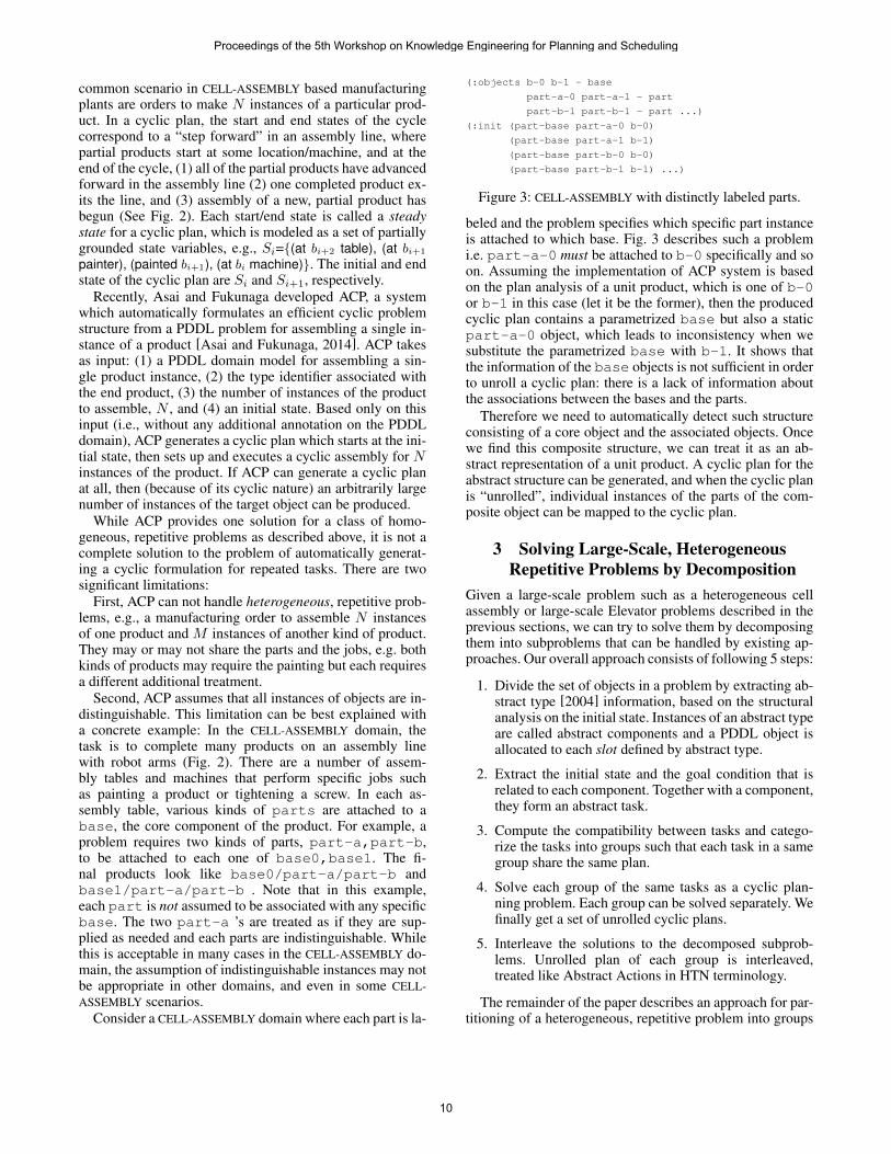
Assuming that once a cyclic plan is generated, themarginal cost of processing an additional product within agroup is almost zero, we can summarize the effect of cate-gorization by comparing the number of components with thenumber of groups of components. Fig. 6(1) shows the result.

The points on the line x = y in Fig. 6(1) shows thatwe cannot get a meaningful categorization in some con-figurations. The reason is twofold: Firstly, the choice ofseed was inappropriate. Indeed, in barman domain, cate-gorization based on cocktail did not result in compo-nents larger than the initial nodes, while that of shot did.This is due to the greedy nature of the abstract type detec-tion algorithm, as described in [Botea, Muller, and Schaef-fer, 2004]. The same thing applies to the results of the otherseed types (though not shown here), such as the decomposi-tion of CELL-ASSEMBLY-EACHPARTS based on arm, table,job and so on. This indicates that restarting the search withall seeds as described in Section 3.1 is required to ensurethat a meaningful categorization is found if one exists. Sec-ondly, in OPENSTACKS, both seeds order and productfailed to get a meaningful information. In this case, the rea-son is attributed to the domain’s characteristics itself i.e. it ispossible that the domain has no inherent meaningful catego-rization.

Evaluation of the Optimization Methods Here we showthe effect of pre-categorization described in Sec. 3.2.Though we are not able to include detailed results here, Fig.6(2) shows the distribution of pre-categorization (based onthe conditions 1 to 3, Sec. 3.2). It shows that the number ofcomparisons that are actually performed is far less than thoserequired by the naive method because most categorizationsare already done i.e. most tasks are already categorized intogroups of a few elements (1 or 2 elements).

We also compare the actual number of calls to the under-lying planner with a naive implementation. In a naive im-plementation, N components require N calls to the planner.Fig. 6(3) shows that the evaluation was reduced by a factorof 2. The results in all domains in Table 1 are shown at once.

Total Elapsed Time of the Categorization Elapsed timeis a key factor when our method is considered as a prepro-cessing step for planning. We show the results in Fig. 6(4).

Unfortunately, some problems are found to take very longtime to compute the categorization due to the heavy objectrestoration (Sec. 3.2). The figure clearly shows that the mosttime-consuming ( t ≈ 105 ) decompositions required thecomponent problems with object restoration 〈D, O, I,GX〉,not by 〈D, OX , IX , GX〉. In Fig. 6(5), we show that the cur-rent bottleneck in solving a restored problem is mainly thePDDL→ SAS converter in Fast Downward. Addressing thisissue remains future work.

5 Related WorksThe overall approach we are pursuing, which is to decom-pose a large problem into relatively easy subproblems, is in-spired by previous work on problem decomposition [Yang,Bai, and Qiu, 1994] and Hierarchical Task Network (HTN)planning [Erol, Hendler, and Nau, 1994]. In HTN, problemdecomposition is done by methods which describes how anabstract-level task can be decomposed into the smaller sub-tasks. It naturally supports the cyclic structure by allowingself-recursive decomposition of compound tasks. Thus, de-composition gives HTN strictly more expressivity than thatof classical planning [1994].

HTN differs from our approach in that methods aremostly written by the human experts, while ours is basedon static problem analysis. However, sevaral approacheshas already been made for learning the methods automati-cally. HTN-MAKER[Hogg, Munoz-Avila, and Kuter, 2008]learns methods from existing plans built by experts and aset of annotated tasks. The learning process works in a hi-erarchical manner. Similarly, LIGHT[Nejati, Langley, andKonik, 2006] system induces methods also from the expertplan but by backward skill chaining from the goal.

Our approach is related to macro abstraction systems suchas Macro-FF [Botea et al., 2005], which automatically iden-tifies reusable plan fragments, and in fact, the componentabstraction framework we extended was originally used byBotea et al to identify macros [Botea, Muller, and Schaeffer,2004]. Macro systems strive to provide a very general ab-straction mechanism, but are typically limited to relativelyshort macros (e.g., 2-step macros in Macro-FF). Our ap-proach, on the other hand, focuses on identifying ‘very longmacros” (10-30 steps per cycle) corresponding to specificabstract tasks.

Another related work is symmetry detection in [Fox andLong, 1999]. It builds symmetry groups of objects and ac-tions by exploiting the initial and goal condition in a givenproblem. The symmetry is incrementally broken during thesearch and the information is used to suppress the branchingfactor, while our method is focused on the preprocessing be-fore the actual search. Also, their work do not consider thestructure of objects, thus shares the similar aspects with ourprevious approach described in Sec. 2.1.

6 ConclusionsThis paper presents preliminary work on a decomposition-based approach for solving large scale planning problemswith a repetitive structure in domains such as factory assem-bly. We presented an overview of our decomposition-based


14

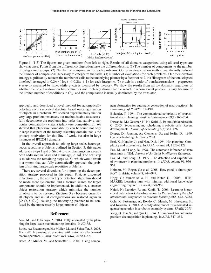
Figure 6: (1-5) The figures are given numbers from left to right. Results of all domains categorized using all seed types areshown at once. Points from the different configuration have the different density. (1) The number of components vs the numberof categorized groups. (2) Number of comparisons for each problems. Our pre-categorization method significantly reducedthe number of comparisons necessary to categorize the tasks. (3) Number of evaluations for each problems. Our memoizationstrategy significantly reduces the number of calls to the underlying planner by a factor of≈ 2. (4) Histogram of the total elapsedtime[sec], averaged in 0.2n ≤ log t ≤ 0.2(n + 1) for each integer n. (5) x-axis is a ratio of translate/(translate + preprocess+ search) measured by time, while y-axis is measured by memory. We show the results from all the domains, regardless ofwhether the object restoration has occured or not. It clearly shows that the search in a component problem is easy because ofthe limited number of conditions in GX , and the computation is usually dominated by the translator.

approach, and described a novel method for automaticallydetecting such a repeated structure, based on categorizationof objects in a problem. We showed experimentally that onvery large problem instances, our method is able to success-fully decompose the problems into tasks that satisfy a par-ticular compatibility criteria (plan-wise compatibility). Weshowed that plan-wise compatibility can be found not onlyin large instances of the factory assembly domain that is theprimary motivation for this line of work, but also in largeinstances of IPC2011 domains.

In the overall approach to solving large-scale, heteroge-neous repetitive problems outlined in Section 3, this paperaddresses Steps 1 and 3. Step 4 (cyclic planning) has alreadybeen addressed in [Asai and Fukunaga, 2014]. The next stepis to address the remaining steps (2, 5), which would resultin a system that can fully automatically approach the prob-lem of solving large-scale repetitive problems.

There are several directions for improving the decompo-sition strategy proposed in this paper. First, as discussedin Section 3.1, the abstract type detection algorithm shouldbe made more systematic, and a focused search for largercomponents should be implemented. In addition, a smarterobject restoration strategy which minimize the numberof objects to be restored (Section 3.2) because currentlyall objects and initial configurations are restored again in〈D, O, I,GX〉, causing the underlying planner to be con-fused by the unnecessarily large number of objects.

ReferencesAsai, M., and Fukunaga, A. 2014. Fully automated cyclic plan-ning for large-scale manufacturing domains. In ICAPS.

Botea, A.; Enzenberger, M.; Muller, M.; and Schaeffer, J. 2005.Macro-ff: Improving ai planning with automatically learnedmacro-operators. J. Artif. Intell. Res.(JAIR) 24:581–621.

Botea, A.; Muller, M.; and Schaeffer, J. 2004. Using compo-

nent abstraction for automatic generation of macro-actions. InProceedings of ICAPS, 181–190.Bylander, T. 1994. The computational complexity of proposi-tional strips planning. Artificial Intelligence 69(1):165–204.Dawande, M.; Geismar, H. N.; Sethi, S. P.; and Sriskandarajah,C. 2005. Sequencing and scheduling in robotic cells: Recentdevelopments. Journal of Scheduling 8(5):387–426.Draper, D.; Jonsson, A.; Clements, D.; and Joslin, D. 1999.Cyclic scheduling. In Proc. IJCAI.Erol, K.; Hendler, J.; and Nau, D. S. 1994. Htn planning: Com-plexity and expressivity. In AAAI, volume 94, 1123–1128.Fox, M., and Long, D. 1998. The automatic inference of stateinvariants in TIM. Journal of Artificial Intelligence Research.Fox, M., and Long, D. 1999. The detection and exploitationof symmetry in planning problems. In IJCAI, volume 99, 956–961.Helmert, M.; Roger, G.; et al. 2008. How good is almost per-fect?. In AAAI, volume 8, 944–949.Hogg, C.; Munoz-Avila, H.; and Kuter, U. 2008. HTN-MAKER: Learning htns with minimal additional knowledgeengineering required. In AAAI, 950–956.Nejati, N.; Langley, P.; and Konik, T. 2006. Learning hierar-chical task networks by observation. In Proceedings of the 23rdinternational conference on Machine learning, 665–672. ACM.Ochi, K.; Fukunaga, A.; Kondo, C.; Maeda, M.; Hasegawa, F.;and Kawano, Y. 2013. A steady-state model for automated se-quence generation in a robotic assembly system. SPARK 2013.Yang, Q.; Bai, S.; and Qiu, G. 1994. A framework for automaticproblem decomposition in planning. In AIPS, 347–352.


15

Eliminating All Redundant Actions from Plans Using SAT and MaxSAT

Tomas BalyoDepartment of Theoretical Computer Science

and Mathematical Logic,Faculty of Mathematics and Physics

Charles University in [email protected]

Lukas ChrpaPARK Research Group

School of Computing and EngineeringUniversity of Huddersfield

[email protected]

Abstract

Satisfiability (SAT) techniques are often successfullyused for solving planning problems. In this paper weshow, that SAT and maximum satisfiability (MaxSAT)can be also used for post-processing optimization ofplans. We will restrict ourselves to improving plans byremoving redundant actions from them which is a spe-cial case of plans optimization. There exist polynomialalgorithms for removing redundant actions, but noneof them can remove all such actions since guarantee-ing that a plan does not contain redundant actions isNP-complete. We introduce two new algorithms, basedon SAT and MaxSAT, which remove all redundant ac-tions. The MaxSAT based algorithm additionally guar-antees to remove a maximum set of redundant actions.We test the described algorithms on plans obtained bystate-of-the-art planners on IPC 2011 benchmarks. Theproposed algorithms are very fast for these plans despitethe complexity results.

IntroductionAutomated Planning is an important research area for itsgood application potential (Ghallab, Nau, and Traverso2004). With intelligent systems becoming ubiquitous thereis a need for planning systems to operate in almost real-time.Sometimes it is necessary to provide a solution in a very lit-tle time to avoid imminent danger (e.g damaging a robot)and prevent significant financial losses. Satisficing planningengines such as FF (Hoffmann and Nebel 2001), Fast Down-ward (Helmert 2006) or LPG (Gerevini, Saetti, and Serina2003) are often able to solve a given problem quickly, how-ever, quality of solutions might be low. Optimal planningengines, which guarantee the best quality solutions, oftenstruggle even on simple problems. Therefore, a reasonableway how to improve the quality of the solutions producedby satisficing planning engines is to use post-planning opti-mization techniques.

In this paper we restrict ourselves to optimizing plansby only removing redundant actions from them. Guarantee-ing that a plan does not contain redundant actions is NP-complete (Fink and Yang 1992). There are polynomial al-gorithms, which remove most of the redundant actions, butnone of them removes all such actions. We propose twonew algorithms which are guaranteed to remove them all.

One uses satisfiability (SAT) solving, the other one relies onmaximum satisfiability (MaxSAT) solving. We compare ouralgorithms with a heuristic algorithm on plans obtained bystate-of-the-art planners on IPC 2011 benchmarks.

Related WorkVarious techniques have been proposed for post-planningplan optimization. Westerberg and Levine (2001) proposeda technique based on Genetic Programming, however, it isnot clear whether it is required to hand code optimizationpolicies for each domain as well as how much runtime isneeded for such a technique. Planning Neighborhood GraphSearch (Nakhost and Muller 2010) is a technique which ex-pands a limited number of nodes around each state alongthe plan and then by applying Dijsktra‘s algorithm finds abetter quality (shorter) plan. This technique is anytime sincewe can iteratively increase the limit for expanded nodes inorder to find plans of better quality. AIRS (Estrem and Kreb-sbach 2012) improves quality of plans by identifying subop-timal subsequences of actions according to heuristic estima-tion (a distance between given pairs of states). If the heuris-tic indicates that states might be closer than they are, thena more expensive (optimal) planning technique is used tofind a better sequence of actions connecting the given states.A similar approach exists for optimizing parallel plans (Ba-lyo, Bartak, and Surynek 2012). A recent technique (Sid-diqui and Haslum 2013) uses plan deordering into ‘blocks’of partially ordered subplans which are then optimized. Thisapproach is efficient since it is able to optimize subplanswhere actions might be placed far from each other in a totalyordered plan.

Determining and removing redundant actions from plansis a specific sub-category of post-planning plan optimiza-tion. An influential work (Fink and Yang 1992) defines fourcategories of redundant actions and provides complexity re-sults for each of the categories. One of the categories refersto Greedily justified actions. A greedily justified action inthe plan is, informally said, such an action which if it andactions dependent on it are removed from the plan, the planbecomes invalid. Greedy justification is used in the Ac-tion Elimination (AE) algorithm (Nakhost and Muller 2010)which is discussed in detail later in the text. Another ofthe categories refers to Perfectly Justified plans, plans inwhich no redundant actions can be found. Minimal reduc-


16

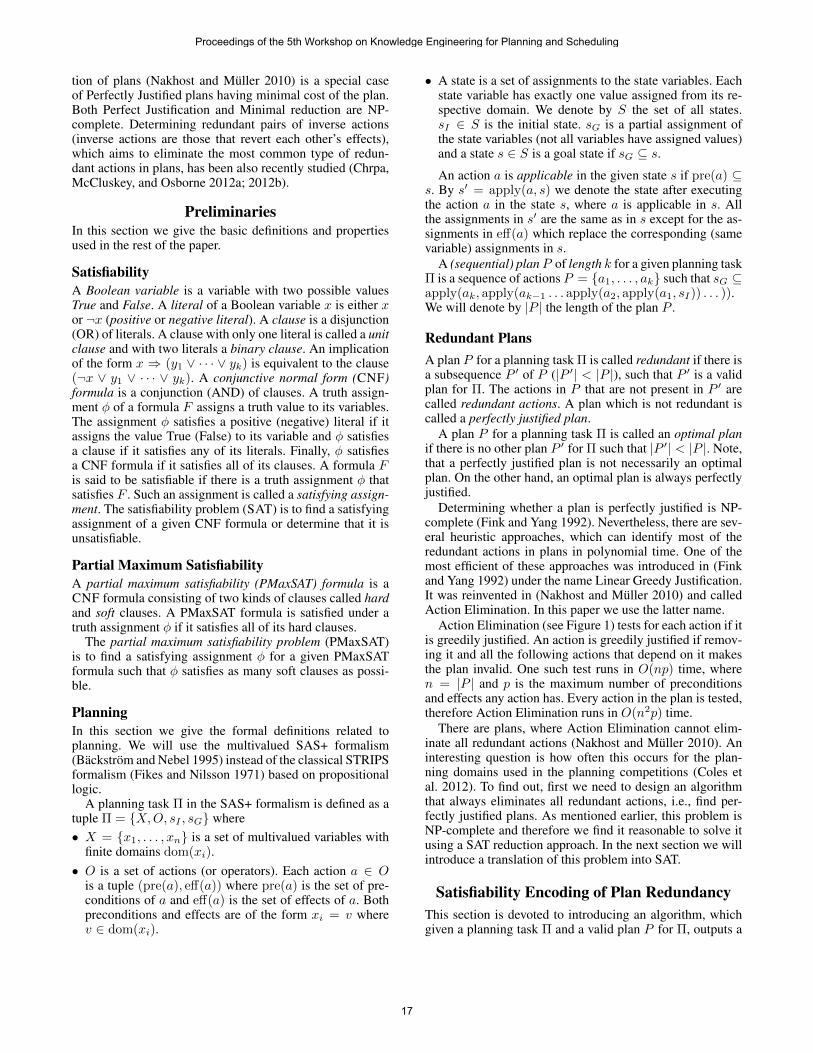
tion of plans (Nakhost and Muller 2010) is a special caseof Perfectly Justified plans having minimal cost of the plan.Both Perfect Justification and Minimal reduction are NP-complete. Determining redundant pairs of inverse actions(inverse actions are those that revert each other’s effects),which aims to eliminate the most common type of redun-dant actions in plans, has been also recently studied (Chrpa,McCluskey, and Osborne 2012a; 2012b).

PreliminariesIn this section we give the basic definitions and propertiesused in the rest of the paper.

SatisfiabilityA Boolean variable is a variable with two possible valuesTrue and False. A literal of a Boolean variable x is either xor ¬x (positive or negative literal). A clause is a disjunction(OR) of literals. A clause with only one literal is called a unitclause and with two literals a binary clause. An implicationof the form x ⇒ (y1 ∨ · · · ∨ yk) is equivalent to the clause(¬x ∨ y1 ∨ · · · ∨ yk). A conjunctive normal form (CNF)formula is a conjunction (AND) of clauses. A truth assign-ment φ of a formula F assigns a truth value to its variables.The assignment φ satisfies a positive (negative) literal if itassigns the value True (False) to its variable and φ satisfiesa clause if it satisfies any of its literals. Finally, φ satisfiesa CNF formula if it satisfies all of its clauses. A formula Fis said to be satisfiable if there is a truth assignment φ thatsatisfies F . Such an assignment is called a satisfying assign-ment. The satisfiability problem (SAT) is to find a satisfyingassignment of a given CNF formula or determine that it isunsatisfiable.

Partial Maximum SatisfiabilityA partial maximum satisfiability (PMaxSAT) formula is aCNF formula consisting of two kinds of clauses called hardand soft clauses. A PMaxSAT formula is satisfied under atruth assignment φ if it satisfies all of its hard clauses.

The partial maximum satisfiability problem (PMaxSAT)is to find a satisfying assignment φ for a given PMaxSATformula such that φ satisfies as many soft clauses as possi-ble.

PlanningIn this section we give the formal definitions related toplanning. We will use the multivalued SAS+ formalism(Backstrom and Nebel 1995) instead of the classical STRIPSformalism (Fikes and Nilsson 1971) based on propositionallogic.

A planning task Π in the SAS+ formalism is defined as atuple Π = {X,O, sI , sG} where• X = {x1, . . . , xn} is a set of multivalued variables with

finite domains dom(xi).• O is a set of actions (or operators). Each action a ∈ O

is a tuple (pre(a), eff(a)) where pre(a) is the set of pre-conditions of a and eff(a) is the set of effects of a. Bothpreconditions and effects are of the form xi = v wherev ∈ dom(xi).

• A state is a set of assignments to the state variables. Eachstate variable has exactly one value assigned from its re-spective domain. We denote by S the set of all states.sI ∈ S is the initial state. sG is a partial assignment ofthe state variables (not all variables have assigned values)and a state s ∈ S is a goal state if sG ⊆ s.An action a is applicable in the given state s if pre(a) ⊆

s. By s′ = apply(a, s) we denote the state after executingthe action a in the state s, where a is applicable in s. Allthe assignments in s′ are the same as in s except for the as-signments in eff(a) which replace the corresponding (samevariable) assignments in s.

A (sequential) planP of length k for a given planning taskΠ is a sequence of actions P = {a1, . . . , ak} such that sG ⊆apply(ak, apply(ak−1 . . . apply(a2, apply(a1, sI)) . . . )).We will denote by |P | the length of the plan P .

Redundant PlansA plan P for a planning task Π is called redundant if there isa subsequence P ′ of P (|P ′| < |P |), such that P ′ is a validplan for Π. The actions in P that are not present in P ′ arecalled redundant actions. A plan which is not redundant iscalled a perfectly justified plan.

A plan P for a planning task Π is called an optimal planif there is no other plan P ′ for Π such that |P ′| < |P |. Note,that a perfectly justified plan is not necessarily an optimalplan. On the other hand, an optimal plan is always perfectlyjustified.

Determining whether a plan is perfectly justified is NP-complete (Fink and Yang 1992). Nevertheless, there are sev-eral heuristic approaches, which can identify most of theredundant actions in plans in polynomial time. One of themost efficient of these approaches was introduced in (Finkand Yang 1992) under the name Linear Greedy Justification.It was reinvented in (Nakhost and Muller 2010) and calledAction Elimination. In this paper we use the latter name.

Action Elimination (see Figure 1) tests for each action if itis greedily justified. An action is greedily justified if remov-ing it and all the following actions that depend on it makesthe plan invalid. One such test runs in O(np) time, wheren = |P | and p is the maximum number of preconditionsand effects any action has. Every action in the plan is tested,therefore Action Elimination runs in O(n2p) time.

There are plans, where Action Elimination cannot elim-inate all redundant actions (Nakhost and Muller 2010). Aninteresting question is how often this occurs for the plan-ning domains used in the planning competitions (Coles etal. 2012). To find out, first we need to design an algorithmthat always eliminates all redundant actions, i.e., find per-fectly justified plans. As mentioned earlier, this problem isNP-complete and therefore we find it reasonable to solve itusing a SAT reduction approach. In the next section we willintroduce a translation of this problem into SAT.

Satisfiability Encoding of Plan RedundancyThis section is devoted to introducing an algorithm, whichgiven a planning task Π and a valid plan P for Π, outputs a


17

ActionElimination (Π, P )AE01 s := sIAE02 i := 1AE03 repeatAE04 mark(ai)AE05 s′ := sAE06 for j := i+ 1 to |P | doAE07 if applicable(aj , s′) thenAE08 s′ := apply(aj , s′)AE09 elseAE10 mark(aj)AE11 if goalSatisfied(s′) thenAE12 P := removeMarked(P )AE13 elseAE14 unmarkAllActions()AE15 s := apply(ai, s)AE16 i := i+ 1AE17 until i > |P |AE18 return P

Figure 1: Pseudo-code of the Action Elimination algorithmas presented in (Nakhost and Muller 2010).

CNF formula FΠ,P , such that FΠ,P is satisfiable if and onlyif P is a redundant plan for Π.

We provide several definitions which are required to un-derstand the concept of our approach. An action a is calleda supporting action for a condition c if c ∈ eff(a). An ac-tion a is an opposing action of a condition c := xi = vif xi = v′ ∈ eff(a) where v 6= v′. The rank of an actiona in a plan P is its order in the sequence P . We will de-note by Opps(c, i, j) the set of ranks of opposing actionsof the condition c which have their rank between i and j(i ≤ j). Similarly, by Supps(c, i) we will mean the set ofranks of supporting actions of the condition c which haveranks smaller than i.

In our encoding we will have two kinds of variables. First,we will have one variable for each action in the plan P ,which will represent whether the action is required for theplan. We will say that ai = True if the i-th action of P (theaction with the rank i) is required. The second kind of vari-ables will be option variables, their purpose and meaning isdescribed below.

The main idea of the translation is to encode the fact, thatif a certain condition ci is required to be true at some time iin the plan, then one of the following must hold:

• The condition ci is true since the initial state and there isno opposing action of ci with a rank smaller than i.

• There is a supporting action aj of ci with the rank j andthere is no opposing action of ci with the rank between jand i.

These two kinds of properties represent the options for sat-isfying ci. There is at most one option of the first kind and atmost |P | of the second kind. For each one of them we willuse a new option variable yc,i,k, which will be true if thecondition c at time i is satisfied using the k-th option.

Now we demonstrate how to encode the fact, that we re-quire condition c to hold at time i. If c is in the initial state,then the first option will be expressed using the followingconjunction of clauses.

Fc,i,0 =∧

j∈Opps(c,0,i)

(¬yc,i,0 ∨ ¬aj)

These clauses are equivalent to the implications below. Theimplications represent that if the given option is true, thennone of the opposing actions can be true.

(yc,i,0 ⇒ ¬aj);∀j ∈ Opps(c, 0, i)For each supporting action aj (j ∈ Supps(c, i)) with rankj we will introduce an option variable yc,i,j and add the fol-lowing subformula.

Fc,i,j = (¬yc,i,j ∨ aj)∧

k∈Opps(c,j,i)

(¬yc,i,j ∨ ¬ak)

These clauses are equivalent to the implications that if thegiven option is true, then the given supporting action is trueand all the opposing actions located between them are false.Finally, for the condition c to hold at time i we need to addthe following clause, which enforces at least one option vari-able to be true.

Fc,i = (yc,i,0∨

j∈Supps(c,i)

yc,i,j)

Using the encoding of the condition requirement it is noweasy to encode the dependencies of the actions from the in-put plan and the goal conditions of the problem. For an ac-tion ai with the rank i we will require that if this action vari-able is true, then all of its preconditions must be true at timei. For an action ai the following clauses will enforce, thatif the action variable is true, then all the preconditions musthold.

Fai =∧

c∈pre(ai)

(¬ai ∨ Fc,i) ∧ Fc,i,0∧

j∈Supps(c,i)

Fc,i,j

We will need to add these clauses for each action in the plan.Let us call these clauses FA.

FA =∧ai∈P

Fai

For the goal we will just require all the goal conditions tobe true in the end of the plan. Let n = |P |, then the goalconditions are encoded using the following clauses.

FG =∧c∈sG

Fc,n ∧ Fc,n,0 ∧j∈Supps(c,n)

Fc,n,j

The last clause we need to add is related to the redundancy

property of the plan. The following clause is satisfied if atleast one of the actions in the plan is omitted.

FR =

( ∨ai∈P

¬ai

)


18

Finally, the whole formula FΠ,P consists of the redun-dancy clause, the goal clauses, and the action dependencyclauses for each action in P .

FΠ,P = FR ∧ FG ∧ FA

If the formula is satisfiable, we also want to use its sat-isfying assignment to construct a new reduced plan. A planobtained using a truth assignment φ will be denoted as Pφ.We define Pφ to be a subsequence of P such that the i-thaction of P is present in Pφ if and only if φ(ai) = True.

Lemma 1. An assignment φ satisfies FG ∧FA if and only ifPφ is a valid plan for Π.

Proof. (sketch) A plan is valid if all the actions in it are ap-plicable when they should be applied and the goal conditionsare satisfied in the end. We constructed the clauses of FG toenforce that at least one option of satisfying each conditionwill be true. The selected option will then force the requiredaction and none of its opposing actions to be in the plan. Us-ing the same principles, the clauses in FA guarantee that ifan action is present in the plan, then all its preconditions willhold when the action is applied.

Proposition 1. The formula FΠ,P is satisfiable if and onlyif P is a redundant plan for Π.

Proof. The clause FR is satisfied by an assignment φ if andonly if at least one ai is false, i.e., not present in Pφ whichimplies |Pφ| < |P |. Using the previous lemma, we can con-clude, that the entire formula FΠ,P = FR ∧ FG ∧ FA issatisfied of and only if there is a valid plan, which can beobtained from P by omitting at least one of its actions.

Let us conclude this section by computing the followingupper bound on the size of the formula FΠ,P .

Proposition 2. Let p be the maximum number of precondi-tions of any action in P ,g the number of goal conditionsof Π, and n = |P |. Then the formula FΠ,P has at mostn2p+ng+n variables and n3p+n2g+np+g+1 clauses,from which n3p+ n2g are binary clauses.

Proof. The are n action variables. For each required condi-tion we have at most n option variables, since there are atmost n supporting actions for any condition in the plan. Wewill require at most (g + np) conditions for the g goal con-ditions and the n actions with at most p preconditions each.Therefore the total number of option variables is n(np+ g).

For the encoding of each condition at any time we useat most n options. Each of these options are encoded us-ing n binary clauses (the are at most n opposing actions forany condition). Additionally we have one long clause sayingthat at least one of the options must be true. We have np re-quired conditions because of the actions and g for the goalconditions. Therefore in total we have at most (np + g)n2

binary clauses and (np+ g) longer clauses related to condi-tions. There is one additional long clause – the redundancyclause.

Making Plans Perfectly JustifiedIn this section we describe how to use the encoding de-scribed in the previous section to convert any given plan intoa perfectly justified plan.

The idea is very similar to the standard planning as SATapproach (Kautz and Selman 1992), where we repeatedlyconstruct formulas and call a SAT solver until we find a plan.In this case we start with a plan, and keep improving it bySAT calls until it is perfectly justified.

RedundancyElimination (Π, P )I1 FΠ,P := encodeRedundancy(Π, P )I2 while isSatisfiable(FΠ,P ) doI3 φ := getSatAssignment(FΠ,P )I4 P := PφI5 FΠ,P := encodeRedundancy(Π, P )I6 return P

Figure 2: Pseudo-code of the SAT based redundancy elimi-nation algorithm. It returns a perfectly justified plan.

The algorithm’s pseudo-code is presented in Figure 2. Ituses a SAT solver to determine whether a plan is perfectlyjustified or it can be improved. It can be improved if theformula FΠ,P is satisfiable. In this case a new plan is con-structed using the satisfying assignment. The while loop ofthe algorithm runs at most |P | times, since every time at leastone action is removed from P (in practice several actions areremoved in each step).

The algorithm can be implemented in a more efficientmanner if we have access to an incremental SAT solver. Weneed the simplest kind of incrementality – adding clauses.

IncrementalRedundancyElimination (Π, P )II01 solver = new SatSolverII02 solver.addClauses(encodeRedundancy(Π, P ))II03 while solver.isSatisfiable() doII04 φ := solver.getSatAssignment()II06 C :=

∨{¬ai|ai ∈ Pφ}

II07 solver.addClause(C)II08 foreach ai ∈ P do if φ(ai) = False thenII09 solver.addClause({¬ai})II10 P := PφII11 return P

Figure 3: Pseudo-code of the incremental SAT based redun-dancy elimination algorithm.

The incremental algorithm is presented in Figure 3. Itadds a new clause C in each iteration of the while loop.This clause is a redundancy clause for the actions remainingin the current plan. It will enforce, that the next satisfyingassignment will remove at least one further action. The re-dundancy clauses added in the previous iterations could beremoved, but it is not necessary. The algorithm also adds unitclauses to enforce that the already eliminated actions cannotbe reintroduced.


19

The algorithms presented in this section are guaranteed toproduce plans that are perfectly justified, i.e., it is not possi-ble to remove any further actions from them. Nevertheless,it might be the case, that if we had removed a different setof redundant actions from the initial plan, we could have ar-rived at a shorter perfectly justified plan. In other words, theelimination of redundancy is not confluent. The followingexample demonstrates this fact.

Example 1. Let us have a simple path planning scenarioon a graph with n vertices v1, . . . , vn and edges (vi, vi+1)for each i < n and (vn, v1) to close the circle. We have oneagent traveling on the graph from v1 to vn. We have twomove actions for each edge (for both directions), in total 2nmove actions. The optimal plan for the agent is a one actionplan {move(v1, vn)}.

Let us assume that we are given the following planfor redundancy elimination: {move(v1, vn), move(vn, v1),move(v1, v2), move(v2, v3), . . ., move(vn−1, vn)}.

The plan can be made perfectly justified by either remov-ing all but the first action (and obtaining the optimal plan)or by removing the first two actions (ending up a with a planof n actions). Action elimination would remove the first twoactions, for the SAT algorithm we cannot tell which actionswould be removed, it depends on the satisfying assignmentthe SAT solver returns.

The example shows us, that it matters very much in whatorder we remove the actions and achieving perfect justifica-tion does not necessarily mean we did a good job. What weactually want is to remove as many actions as possible. Howto do this efficiently is described in the next section.

Maximum Redundancy EliminationIn the section we describe how to do the best possible re-dundancy elimination for a plan. The problem of maximumredundancy elimination (MRE) is to find a subsequence Rof redundant actions in a plan P , such that there is no othersubsequenceR′ of redundant actions which is longer thanR.A similar notion (minimal reduction) was defined for planswith actions costs (Nakhost and Muller 2010).

The plan resulting from MRE is always perfectly justified,on the other hand a plan might be perfectly justified and atthe same time much longer than a plan obtained by MRE(see Example 1).

The solution we propose for MRE is also based on ourredundancy encoding, but instead of a SAT solver we willuse a partial maximum satisfiability (PMaxSAT) solver. Wewill construct a PMaxSAT formula, which is very similar tothe formula used for redundancy elimination.

A PMaxSAT formula consists of hard and soft clauses.The hard clauses will be the clauses we used for redundancyelimination without the redundancy clause FR.

HΠ,P = FG ∧ FAThe soft clauses will be unit clauses containing the negationsof the action variables.

SΠ,P =∧ai∈P

(¬ai)

The PMaxSAT solver will find an assignment φ that satisfiesall the hard clauses (which enforces the validity of the planPφ due to Lemma 1) and satisfies as many soft clauses aspossible (which removes as many actions as possible).

MaximumRedundancyEliminaion (Π, P )MR1 F := encodeMaximumRedundancy(Π, P )MR2 φ := partialMaxSatSolver(F )MR3 return Pφ

Figure 4: Pseudo-code of the maximum redundancy elimi-nation algorithm.

The algorithm (Figure 4) is now very simple and straight-forward. We just construct the formula and use a PMaxSATsolver to obtain an optimal satisfying assignment. Using thisassignment we construct an improved plan the same way aswe did in the SAT based redundancy elimination algorithm.

Experimental EvaluationIn this section we present the results of our experimentalstudy regarding elimination of redundant actions from plans.We implemented the Action Elimination algorithm as wellas the SAT and MaxSAT based algorithms and used plansobtained by several planners for the problems of the Interna-tional Planning Competition (Coles et al. 2012).

Experimental SettingsSince, our tools take input in the SAS+ format, we usedHelmert’s translation tool, which is a part of the Fast Down-ward planning system (Helmert 2006), to translate the IPCbenchmark problems that are provided in PDDL.

To obtain the initial plans, we used the following state-of-the-art planners: FastDownward (Helmert 2006), Metric FF(Hoffmann 2003), and Madagascar (Rintanen 2013). Eachof these planners was configured to find plans as fast as pos-sible and ignore plan quality.

We tested four redundancy elimination methods:• Action Elimination (AE) is our own Java implementation

of the Action Elimination algorithm as displayed in Fig-ure 1.

• Action Elimination + SAT (AE+S) is an algorithm thatfirst runs Action Elimination on the initial plan and in-cremental SAT reduction (see Figure 3) on the result. Weused the incremental Java SAT solver Sat4j (Berre andParrain 2010).

• SAT Reduction (SAT) is using the incremental SAT reduc-tion directly without using Action Elimination for prepro-cessing (same as AE+S without AE).

• Maximum Elimination (MAX) is a Partial MaxSAT reduc-tion based algorithm displayed in Figure 4. We imple-mented the translation in Java and used the QMaxSAT(Koshimura et al. 2012) state-of-the-art MaxSAT solverwritten in C++ to solve the instances.

For each of these methods we measured the total runtimeand the total number of removed redundant actions for eachdomain and planner.


20

Table 1: Experimental results on the plans for the IPC 2011 domains found by the planners Fast Downward, Metric FF, andMadagascar. The planners were run with a time limit of 10 minutes. The column ”#Plans” contains the number of plans foundand ”Length” represents the sum of their lengths. By ∆ALG and TALG we mean the total number of removed redundant actionsand the time in seconds it took for all plans for a given algorithm ALG. The algorithms are Action Elimination (AE), ActionElimination followed by SAT reduction (AE+S), SAT reduction on the original plan (SAT), and maximum elimination using aMaxSat solver (MAX).

Domain #Plans Length ∆AE TAE ∆AE+S TAE+S ∆SAT TSAT ∆MAX TMAX

Met

ric

FF

elevators 20 4273 79 0,81 79 2,31 79 3,14 79 0,17floortile 2 81 10 0,02 10 0,08 10 0,10 10 0,00nomystery 5 107 0 0,01 0 0,16 0 0,17 0 0,00parking 18 1546 124 0,18 124 1,13 124 1,60 124 0,03pegsol 20 637 0 0,10 0 1,10 0 1,16 0 0,02scanalyzer 18 571 30 0,06 30 0,78 30 0,88 30 0,01sokoban 13 2504 6 0,39 6 2,34 6 2,52 6 0,36tidybot 17 1136 144 0,17 144 0,92 144 1,66 144 0,04transport 6 1329 164 0,34 164 0,82 164 2,15 165 0,25visitall 3 1137 166 0,14 166 0,47 166 0,97 172 0,08woodworking 19 1471 22 0,37 22 1,14 22 1,28 22 0,02

Fast

Dow

nwar

d

barman 20 3749 528 0,52 582 3,44 596 7,18 629 0,44elevators 20 4625 94 0,84 94 2,41 94 3,45 94 0,19floortile 5 234 22 0,06 22 0,20 22 0,27 22 0,00nomystery 13 451 0 0,05 0 0,47 0 0,48 0 0,00parking 20 1494 4 0,17 4 1,21 4 1,26 4 0,03pegsol 20 644 0 0,11 0 1,11 0 1,18 0 0,02scanalyzer 20 823 26 0,10 26 1,16 26 1,33 26 0,03sokoban 17 5094 244 0,62 458 5,25 458 8,39 460 1,84tidybot 16 1046 64 0,14 64 0,91 64 1,28 64 0,03transport 17 4059 289 0,65 289 1,64 289 2,93 290 0,20visitall 20 28776 122 3,66 122 9,47 122 12,89 122 7,77woodworking 20 1605 27 0,41 27 1,16 27 1,33 30 0,03

Mad

agas

car

barman 8 1785 303 0,25 303 1,59 303 3,53 318 0,30elevators 20 11122 2848 1,46 3017 4,13 3021 17,62 3138 2,03floortile 20 1722 30 0,39 30 1,05 30 1,32 30 0,03nomystery 15 480 0 0,06 0 0,51 0 0,53 0 0,01parking 18 1663 152 0,20 152 1,17 152 1,78 152 0,03pegsol 19 603 0 0,09 0 1,06 0 1,10 0 0,01scanalyzer 18 1417 232 0,24 232 0,88 232 1,61 236 0,05sokoban 1 121 22 0,02 22 0,13 22 0,29 22 0,01tidybot 16 1224 348 0,16 348 0,84 348 2,13 350 0,08transport 4 1446 508 0,20 539 0,40 532 1,65 553 0,16woodworking 20 1325 0 0,31 0 1,11 0 1,21 0 0,01


21

All the experiments were run on a computer with IntelCore i7 960 CPU @ 3.20 GHz processor and 24 GB of mem-ory. The planners had a time limit of 10 minutes to find theinitial plans. The benchmark problems are taken from thesatisficing track of IPC 2011 (Coles et al. 2012).

Experimental ResultsThe results of our experiments are displayed in Table 1. Wecan immediately notice that the runtime of all of our meth-ods is very low. None of the methods takes more than onesecond on average for any of the plans. Note, that the run-time of the MAX method is often the smallest contrary tothe fact, that it is the only one which guarantees eliminatingthe maximum number of redundant actions (AE+S and SATonly guarantee perfect justification).

Looking at the number of removed actions in Table 1we can make several interesting observations. For exam-ple, in the nomystery and pegsol domains no redundant ac-tions were found in plans obtained by any planner and alsoMadagascar’s plans for the woodworking domain were al-ways perfectly justified. In the most cases the AE algorithmprovides perfectly justified plans (this is when the values of∆AE and ∆AE+S are equal). The SAT method performsbetter than AE+S on barman for Fast Downward and ele-vators for Madagascar, but removes less actions on trans-port for Madagascar. Although both methods reach perfectjustification, the results are different since removing redun-dant actions is not confluent (see example 1). As expected,the MAX method removes the highest (or equal) number ofactions in each case. It is strictly dominant for 11 plannerdomain combinations. Considering the good runtime perfor-mance of this method we can conclude, that MAX is the bestway of eliminating redundant actions.

ConclusionsIn this paper, we have introduced a SAT encoding for theproblem of detecting redundant actions in plans and used itto build two algorithms for plan optimization. One is basedon SAT solving and the other on partial MaxSAT solving.Contrary to existing algorithms, both of our algorithms guar-antee, that they output a plan with no redundant actions. Ad-ditionally, the MaxSAT based algorithm always eliminates amaximum set of redundant actions. According to our experi-ments done on IPC benchmark problems with plans obtainedby state-of-the-art planners, our newly proposed algorithmsperform very well in practice.

Acknowledgments The research is supported by theCzech Science Foundation under the contract P103/10/1287and by the Grant Agency of Charles University under con-tract no. 600112. This research was also supported by theSVV project number 260 104.

ReferencesBackstrom, C., and Nebel, B. 1995. Complexity results forsas+ planning. Computational Intelligence 11:625–656.Balyo, T.; Bartak, R.; and Surynek, P. 2012. Shorteningplans by local re-planning. In Proceedings of ICTAI, 1022–1028.

Berre, D. L., and Parrain, A. 2010. The sat4j library, release2.2. JSAT 7(2-3):59–64.Chrpa, L.; McCluskey, T. L.; and Osborne, H. 2012a. De-termining redundant actions in sequential plans. In Proceed-ings of ICTAI, 484–491.Chrpa, L.; McCluskey, T. L.; and Osborne, H. 2012b. Op-timizing plans through analysis of action dependencies andindependencies. In Proceedings of ICAPS, 338–342.Coles, A. J.; Coles, A.; Olaya, A. G.; Celorrio, S. J.; Lopez,C. L.; Sanner, S.; and Yoon, S. 2012. A survey of the seventhinternational planning competition. AI Magazine 33(1).Estrem, S. J., and Krebsbach, K. D. 2012. Airs: Anytimeiterative refinement of a solution. In Proceedings of FLAIRS,26–31.Fikes, R., and Nilsson, N. J. 1971. Strips: A new approachto the application of theorem proving to problem solving.Artif. Intell. 2(3/4):189–208.Fink, E., and Yang, Q. 1992. Formalizing plan justifications.In In Proceedings of the Ninth Conference of the CanadianSociety for Computational Studies of Intelligence, 9–14.Gerevini, A.; Saetti, A.; and Serina, I. 2003. Planningthrough stochastic local search and temporal action graphs.Journal of Artificial Intelligence Research (JAIR) 20:239 –290.Ghallab, M.; Nau, D.; and Traverso, P. 2004. AutomatedPlanning: Theory and Practice. Morgan Kaufmann Pub-lishers.Helmert, M. 2006. The fast downward planning system.Journal of Artificial Intelligence Research (JAIR) 26:191–246.Hoffmann, J., and Nebel, B. 2001. The FF planning system:Fast plan generation through heuristic search. Journal ofArtificial Intelligence Research 14:253–302.Hoffmann, J. 2003. The Metric-FF planning system:Translating ”ignoring delete lists” to numeric state variables.Journal Artificial Intelligence Research (JAIR) 20:291–341.Kautz, H. A., and Selman, B. 1992. Planning as satisfiabil-ity. In Proceedings of ECAI, 359–363.Koshimura, M.; Zhang, T.; Fujita, H.; and Hasegawa, R.2012. Qmaxsat: A partial max-sat solver. JSAT 8(1/2):95–100.Nakhost, H., and Muller, M. 2010. Action elimination andplan neighborhood graph search: Two algorithms for planimprovement. In Proceedings of ICAPS, 121–128.Rintanen, J. 2013. Planning as satisfiability: state of the art.http://users.cecs.anu.edu.au/ jussi/satplan.html.Siddiqui, F. H., and Haslum, P. 2013. Plan quality optimisa-tion via block decomposition. In Proceedings of IJCAI.Westerberg, C. H., and Levine, J. 2001. Optimising plansusing genetic programming. In Proceedings of ECP, 423–428.


22

Planning with Preferences by Compiling Soft Always Goals intoSTRIPS with Action Costs

Luca Ceriani and Alfonso Emilio Gerevini∗Department of Information Engineering, University of Brescia, Italy

[email protected], [email protected] (∗corresponding author)

Abstract

We address the problem of planning with preferences inpropositional domains focusing on soft always goals (or con-straints), a basic class of temporally extended goals useful toexpress maintenance goals, safety conditions, or other desiredconditions that affect the quality of the solution plans. In-spired by previous work of Keyder and Geffner on compilingsoft goals, we propose a compilation scheme for translating aSTRIPS problem with soft always constraints into an equiva-lent STRIPS problem with action costs. This problem trans-formation allows to solve propositional planning problemsenriched with soft always constraints (possibly extendablealso with soft goals) using several existing powerful planners,that need to support only STRIPS and action costs. An ex-perimental analysis presented in the paper demonstrates thatsolving the compiled problems using existing STRIPS plan-ners can be significantly more effective than solving the orig-inal uncompiled problems using planners supporting soft al-ways constraints, such as HPlan-P and MIPS-XXL, in termsof satisfied always constraints and scalability.

IntroductionPlanning with preferences, also called “over-subscriptionplanning” (e.g., (van den Briel et al. 2004; Do and Kamb-hampati 2004; Smith 2004)), is a recent important area ofautomated planning concerning the generation of plans forproblems involving soft goals or state-trajectory constraints,that it is desired a solution plan satisfies, but that do not haveto be necessarily satisfied. The quality of a solution plan forthese problems depends on the soft goals and constraints thatare satisfied by the plan.

In the standard planning language PDDL3 (Gerevini et al.2009), state-trajectory constraints are particular linear tem-poral logic formulae expressing temporally extended goals(Bacchus and Kabanza 1998; Baier and McIlraith 2006)restricting the intermediate states reachable by the validplans. A basic class of state-trajectory constraints con-sists of always constraints (or always goals) expressing thata certain condition must hold in every state reached bya valid plan.1 Adding always constraints to the standard“achievement” goals of a problem (requiring the goals to

1In the literature, always constraints/goals are also called“safety goals”, “maintenance goals”, “state invariants” or “stateconstraints”.

hold at the end of the plan) is useful to express safety ormaintenance conditions (e.g., (Bacchus and Kabanza 1998;Weld and Etzioni 1994)) as well as desired plan proper-ties. Examples of such conditions are “whenever a build-ing surveillance robot is outside a room, all the room doorsshould be closed” or, in a logistics domain, “whenever atruck is at a location, all goods the truck has to load fromthat location have already been transported there” (for ad-ditional examples see, e.g., (Bacchus and Kabanza 1998;Gerevini et al. 2009; Weld and Etzioni 1994)).

In propositional planning, only few planners supportingsoft always constraints have been developed. The mostprominent of them is planner HPlan-P (Baier and McIlraith2008), which won the “qualitative preference” track of the5th International Planning Competition (IPC), focusing onpropositional planning with soft goals and state-trajectoryconstraints expressed through PDDL3.

STRIPS extended with action costs is a simple lan-guage for propositional planning that many existing power-ful planners support, e.g., LPG (Gerevini, Saetti, and Se-rina 2003), Metric-FF (Hoffmann 2003), Fast Downward(Helmert 2006), and LAMA (Richter and Westphal 2010).Handling action costs is a practically important, basic func-tionality that was required in the satisficing tracks of the lasttwo IPCs. Keyder and Geffner (Keyder and Geffner 2009)showed that any STRIPS problem with soft (achievement)goals can be efficiently compiled into an equivalent STRIPSproblem with action costs.

Inspired by Keyder and Geffner’s work, we propose acompilation scheme for translating a STRIPS problem withsoft always constraints into an equivalent STRIPS problemwith action costs. This problem transformation allows tosolve propositional planning problems enriched with soft al-ways constraints (possibly extendable also with soft goals)using several existing powerful planners.

A preliminary experimental analysis presented in this pa-per shows that solving the compiled problems by LPG,Metric-FF or LAMA can be significantly more effective thansolving the original uncompiled problems using plannerssupporting soft always constraints, in terms of plan quality(i.e., satisfied always constraints) and scalability.

Other approaches to compiling (soft) always constraintshave been proposed. The techniques proposed in (Edelkamp2006; Edelkamp, Jabbar, and Nazih 2006; Baier and McIl-


23

raith 2008; Gerevini et al. 2009) use a language richer thanSTRIPS, requiring conditional effects and numerical flu-ents. Their compilation schemas are very different andbased on representing state-trajectory constraints throughautomata encoded in the compiled problem. Two of theseschemas are implemented in planners HPlan-P and MIPS-XXL (Edelkamp and Jabbar 2008). In the experimentalanalysis of this work, we show that these planners performgenerally less efficiently than the compared STRIPS plan-ners.

Another recent planner supporting soft always constraintsis LPRPG-P (Coles and Coles 2011), which is based on a hy-brid heuristic using relaxed planning graphs and linear pro-gramming. Differently from this system, the investigatedcompilation approach has the advantage of allowing manyplanners (using any heuristic for classical planning) to sup-port always constraints, possibly in addition to compiled softgoals.

The remainder of the paper is organised as follows. Aftersome background and definitions about STRIPS with actioncosts and always constraints, we describe our compilationmethod and its properties. Then we present some experi-mental results and finally we give our conclusions.

STRIPS Planning with Action Costs and SoftAlways Constraints

This section describes the STRIPS model of planning withaction costs, introduces its extension with soft always con-straints, and gives some auxiliary definitions used in the restof the paper.

A STRIPS problem is a tuple 〈F, I,O,G〉 where F is aset of fluents, I ⊆ F and G ⊆ F are the initial state andgoal situation, and O is a set of actions or operators definedover F as follows:

Definition 1. Given a set of fluents F , an operator o ∈ O isa pair 〈Prec(o),Eff(o)〉, where Prec(o) is a sets of atomicformulae over F and Eff(o) is a set of literals over F .Eff(o)+ denotes the set of positive literals in Eff(o); Eff(o)−denotes the set of negative literals in Eff(o).

An action sequence π = 〈a0, . . . , an〉 is applicable ina planning problem P if the actions ai, i ∈ {0 . . . n},are all in O and there exists a sequence of states〈s0, . . . , sn+1〉 such that s0 = I , Prec(ai) ⊆ si and,si+1 = si ∪ Eff(o)+ \ Eff(o)− for i ∈ {0 . . . n}. The appli-cable action sequence π achieves a fluent g, if g ∈ sn+1 andis a (valid) plan for P if it achieves each goal g ∈ G, whichwe indicate with π |= G.

Definition 2. A STRIPS problem with action costs (AC) isa tuple Pc = 〈F, I,O,G, c〉, where P = 〈F, I,O,G〉 is aSTRIPS problem and c is a function c : O → R+

0 , mappingeach operator o ∈ O to a non-negative real number.

The cost of a plan π for a problem Pc is given by:

c(π) =

|π|∑i=0

c(ai)

where c(ai) denotes the cost of the ith action ai in π and |π|is the length of π.

An always constraintA, also called always goal, is a tem-porally extended goal expressing a condition that must holdin the problem initial state and in every state of the sequenceof states produced by applying a valid plan π (Bacchus andKabanza 1998; Gerevini et al. 2009). If this is the case, wesay that π satisfiesA, and we indicate it with π |=a A. With-out loss of generality, in the following we will assume thatthe condition of an always constraint is expressed in CNFform. For brevity, (soft) always constraints will be abbrevi-ated with constraint or SAG (soft always goal).

Definition 3. A STRIPS problem with action costs(AC) and soft always goals (SAG) is a tuple Pu =〈F, I,O,G,AG, c, u〉 where:

• 〈F, I,O,G, c〉 is a STRIPS problem with action costs;• AG = {A1, . . . , Ak | Ai CNF formula over F, i =

1 . . . n}• u : AG → R+

0 , is an utility function mapping each al-ways constraint Ai ∈ AG to its utility value over R+

o .

In the following, STRIPS with AC is denoted bySTRIPS+, and STRIPS with SAG by STRIPS+SAG. The(soft) always constraints A in a STRIPS+SAG problem isdenoted with A = ag1 ∧ . . . ∧ agn, where each agi is aclause of A formed by literals over F .

Definition 4. Let Pu be a STRIPS+SAG problem with a setAG of always constraints. The utility of a plan π solvingPu is the difference between the total utility obtained by theplan and its cost:

u(π) =

∑Ai∈AG:π|=aAi

u(Ai)

− c(π).

The definition of plan utility for STRIPS+SAG is simi-lar to the one given for STRIPS+ with soft goals by Key-der and Geffner (2009). A plan π with utility u(π) for aSTRIPS+SAG problem is optimal when no other plan π′ hasutility u(π′) > u(π). The last two IPCs featured tracks inwhich the objective was to find optimal plans with respect tothe plan “net benefit” captured by the equation of Definition4 applied to the utility of soft (end state) goals instead of softalways constraints.

Definition 5. Given a clause ag = l1 ∨ . . . ∨ ln, theset L(ag) = {li | li is a disjunct of ag} is an equiv-alent set-based definition for ag and L(ag) = {¬li |li is a disjunct of ag} is the literal-complement set of L(ag).

Definition 6. Given an operator o ∈ O of a STRIPS+SAGproblem, Z(o) is the set of literals defined as:

Z(o) = (Prec(o)\{p | ¬p ∈ Eff(o)−})∪Eff(o)+∪Eff(o)−.

Note that the literals in Z(o) hold in any reachable stateresulting from the execution of operator o.

In a STRIPS+SAG problem, we distinguish three types ofoperators that are defined as follows.


24

Definition 7. Given an operator o and a constraint A of aSTRIPS+SAG problem, o is a violation of A if there exists aclause agi of A such that:

L(agi) ⊆ Z(o) ∧ L(agi) 6⊆ Prec(o).

If an operator violates a constraint, the constraint is falsein any state resulting from the application of the operator.The set of constraints in a STRIPS+SAG problem that areviolated by an operator o is denoted with V (o).Definition 8. Given an operator o and a constraint A ofa STRIPS+SAG problem, o is a threat for A if it is not aviolation and there exists a clause agi of A, such that:

L(agi)∩Z(o) 6= ∅∧L(agi)∩Z(o) = ∅∧L(agi) 6⊆ Prec(o).

A clause agi of A satisfying the condition of Definition 8is a threatened clause of A. A threatened constraint (clause)may be falsified by an operator depending on the state wherethe operator is applied. The set of constraint threatened byan operator o is denoted with T (o); the set of constraintclauses threatened by o is denoted with TA(o). Note thatthe last conjunct (L(agi) 6⊆ Prec(o)) in the conditions ofDefinitions 7-8 avoid that an operator o is considered a vio-lation/threat when its preconditions require agi to be alreadyviolated in the state where it is applied. This can be use-ful to optimize the compilation procedure, because it is notnecessary to treat o as a violation/threat if in the conditionsof Definitions 7-8 the first two conjuncts hold and the thirddoes not.Definition 9. Given an operator o and a constraint A of aSTRIPS+SAG problem, o is a safe for A if for all clauses agiof A the following condition holds:

L(agi) ∩ Z(o) 6= ∅ ∨ L(agi) ∩ Z(o) = ∅.

If an operator o of a STRIPS+SAG problem P is safe forevery always constraint of P , we say that the operator is safefor P , and we write this property with Safe(o, P ).

Compilation into STRIPS+Given a STRIPS+SAG problem P , an equivalent STRIPS+problem P ′ can be derived using a transformation methodinspired by (Keyder and Geffner 2009), with significant dif-ferences in the compilation of the operators. For the sake ofsimplicity we will assume that every always constraint of Pis satisfied in the problem initial state.2

The operator transformation schema mentioned in the fol-lowing definition is described after the definition.Definition 10. Given a STRIPS+SAG problem P =〈F, I,O,G,AG, c, u〉, the compiled STRIPS+ problem of Pis P ′ = 〈F ′, I ′, O′, G′, c′〉, with:

2Let X be the set of constraints that are false in the initial states. If X is not empty, it can be handled, e.g., as follows: (a) theoriginal operator set is extended with a new operator oinit suchthat Prec(oinit) = {FalseX}, Eff(oinit) = s and c(oinit) is thesum of the utilities of the constraints in X; (b) s is then revised tocontain only FalseX; (c) the constraints in X are not processed bythe operator compilation scheme. Note that any valid plan is forcedto contain oinit as the first action.

• F ′ = F ∪ AV ∪ D ∪ C ′ ∪ C ′ ∪{normal-mode, end-mode, pause};

• I ′ = I ∪ C ′ ∪ {normal-mode};• G′ = G ∪ C ′;• O′ = {collect(A), forgo(A) | A ∈ AG}∪{end}∪Ocomp;

• c′(o) =

u(A) if o = forgo(A)

c(o) if o ∈ O′′c′′(o) if o ∈ OV ∪OT0 otherwise

where:

• AV =k⋃i=1

{Ai-violated}, k = |AG|;

• D =k⋃i=1

{Ai-doneo1 , . . . , Ai-doneon}, k = |AG| and n

is the number of operators threatening or violating Ai;

• C ′ = {A′ | A ∈ AG};

• C ′ = {A′ | A′ ∈ C ′};

• collect(A) = 〈{end-mode,¬A-violated, A′}, {A′,¬A′}〉;

• forgo(A) = 〈{end-mode, A-violated, A′}, {A′,¬A′}〉;• end = 〈{normal-mode}, {end-mode,¬normal-mode}〉;• O′′ = {〈Pre(o) ∪ {normal-mode,¬pause},Eff(o)〉 | o ∈O and Safe(o, P )};

• Ocomp = O′′ ∪OV ∪OT• OV and OT are the sets of operators generated by the op-

erator transformation schema applied to the operators ofP that violate and threaten, respectively, a constraint ofP .3

• c′′(o) is the cost of an operator o in OV ∪ OT as definedin the operator transformation schema.As in (Keyder and Geffner 2009), for each A ∈ AG the

transformation of P into P ′ adds a dummy hard goal A′to P ′ which can be achieved in two ways: with action col-lect(A), that has cost 0 but requires A to be satisfied, i.e.A-violated is false in the goal-state, or with action forgo(A),that has cost equal to the utility of A and can be performedwhen A is false or, equivalently, when A-violated is true.Moreover, for each constraint exactly one of {collect(A),forgo(A)} can appear in the plan, as both delete their sharedprecondition A′, which no action makes true.

The remainder of this section presents the transformationschema for the operators that threaten or violate a soft al-ways constraint. (Note that safe operators are transformedas described in Definition 10, forming operator set O′′.)Threat operators are not trivial to compile because they mayviolate a constraint in different ways, depending on whichplanning state they are applied to. Each operator o such

3If an operator is both a violation and a threat, the generatedcompiled operators are in OT only.


25

that T (o) 6= ∅ is compiled into a set of new operators(one for each threatened constraint). More specifically, letT (o) = {A1, . . . , Am}, be the set of constraints threatenedby o. Operator o is compiled into a sequence of 2m oper-ators OT (o) = {oA1

, oA1, . . . , oAm

, oAm} such that in any

state s where o can be applied violating a set of constraintsT (o)s ⊆ T (o), the sequence ωT (o) ofm operators inOT (o)defined as follows can be applied:

ωT (o) = 〈o′A1, . . . , o′Am

〉 (1)

where o′Ai= oAi if o violatesAi when applied in s, o′Ai

= oAi

if o does not violate Ai when applied in s, and oAi and oAi

are mutually exclusive, for i ∈ {1 . . .m}. The cost c′′(ot)of an operator ot ∈ OT (o) is defined as follows:

c′′(ot) =

{c(o) if o ∈ {oA1

, oA1}

0 otherwisei.e., exactly one of the operators in ωT (the first) cost equalto the cost of the original domain operator compiled intoOT (o), while the others have cost zero.

Before defining the operators forming OT (o) (and ωT (o))for each threatening operator o, we introduce some notationuseful to simplify the presentation:Definition 11. Given an operator o and a constraint clauseag:• NA(o)ag = {l ∈ L(ag) | ¬l ∈ (Eff(o)+ ∪ Eff(o)−)} is

the set of literals in L(ag) falsified by the effects of o;• AA(o)ag = L(ag) \ NA(o)ag is the set of literals inL(ag) not falsified by the application of o andAA(o)ag ={¬l | l ∈ AA(o)ag} is the literal-complement set ofAA(o)ag .For each operator o threatening a set of constraints

T (o) = {A1, . . . , Am}, the operators of OT (o) are definedas follows.• oA1

:

Prec(oA1) = Prec(o) ∪ {¬pause} ∪

{⋃

ag ∈TA(o)

(l1 ∨ . . . ∨ lp) | {l1, . . . , lp} = AA1(o)ag}

Eff(oA1) = {A1-doneo, pause}• oA1

:

Prec(oA1) = Prec(o) ∪ {¬pause} ∪

{∨

ag ∈TA(o)

(l1 ∧ . . . ∧ lq) | {l1, . . . , lq} = AA1(o)ag}

Eff(oA1) = {A1-doneo, pause, A1-violated}

∀k ∈ [2 . . .m− 1]:• oAk

:

Prec(oAk) = {Ak−1-doneo, pause}∪

{⋃

ag∈TA(o)

(l1 ∨ . . . ∨ lp) | {l1, . . . , lp} = AAk(o)ag}

Eff(oAk) = {Ak-doneo,¬Ak−1-doneo}

• oAk:

Prec(oAk) = {Ak−1-doneo, pause}∪

{∨

ag∈TA(o)

(l1,∧ . . . ∧ lq) | {l1, . . . , lq} = AAk(o)ag}

Eff(oAk) = {Ak-doneo, Ak-violated,¬Ak−1-doneo}

if k = m:• oAm :

Prec(oAm) = {⋃

ag∈TA(o)

(l1 ∨ . . . ∨ lp) | {l1, . . . , lp} =

AAm(o)ag} ∪ {Am−1-doneo, pause}Eff(oAm) = Eff(o) ∪ {¬Am−1-doneo,¬pause}• oAm

:

Prec(oAm) = {

∨ag∈TA(o)

(l1,∧ . . . ∧ lq) | {l1, . . . , lq} =

AAm(o)ag} ∪ {Am−1-doneo, pause}Eff(oAm

) = Eff(o) ∪ {¬Am−1-doneo, Am-violated,¬pause}.The operators of T (o) can be applied only in a sequenceωT (o) defined above. The preconditions of any operator oAi

in ωT (o) require AAi(o)ag to hold in the state where ωT (o)

is applied for at least one ag ∈ TAi(o). If this happens, then

oAi∈ ωT (o) and constraint Ai is violated by ωT (o). Predi-

cate Ai-violated is made true by oAiand is never falsified.

After the end action is applied, Ai-violated serves as a pre-condition of the operator forgo(Ai) that has cost equal to theutility of Ai. The Ai-doneo predicates force the planner tostrictly follow the order in ωT (o), avoiding repetitions. Oncethe planner starts sequence ωT (o) for some o, no other oper-ator o′ 6∈ OT (o) is enabled before the application of ωT (o) iscompleted. Predicate pause serves to this purpose, and onlythe last action in the sequence can falsify it.

Each domain operator o violating a constraint (V (o) 6= ∅)must be compiled as well. However, the compilation schemafor o is simpler than the one shown above for a threaten-ing operator. It is sufficient to add to the effects of o anA-violated predicate for each constraint A ∈ V (o). If such amodified operator is applied, all the constraints it violates arefalsified (making their violated-predicates true) and corre-sponding forgo actions must later be selected by the plannerfor every plan achieving the goals. Notice that an operatoro can simultaneously be a violation and a threat of differ-ent sets of constraints. If an operator o threatening a set ofconstraints also violates a constraint A, effect A-violated isadded to the first pair of operators (oA1

, oA1) in OT (A). The

cost c′′(ov) of an operator ov derived by compiling an origi-nal operator o that violates a constraint (and does not threatany other constraint) is the the same cost c(o) of o.

In the compilation of a threatening operator o, its precon-ditions can be extended by disjunctions of literals. Suchdisjunctions can be simplified by performing (unit) reso-lution over the augmented set of preconditions, discharg-ing the operator if the empty close is generated. Moreover,


26

since negation and disjunction are not allowed in STRIPS, afurther standard “ADL-to-STRIPS” translation (Gazen andKnoblock 1997) can be executed to complete the procedureand generate a STRIPS+ problem.

Compilation PropertiesLet P ′ be the STRIPS+ problem derived by compiling aSTRIPS+SAG problem P . All plans π′ solving P ′ have theform π′ = 〈π′′, end, π′′′〉, where the prefix π′′ is formedby operators of P , ω-sequences of compiled operators asdefined in (1), and compiled constraint violating operatorsof P . Each sequence ωT (o) in π′ corresponds to the applica-tion of an operator o ∈ O of P in an equivalent solution planπ for P . The two problems P and P ′ are equivalent in thesense that there is a correspondence between the plans forP and P ′, and corresponding plans are ranked in the sameway by the utility functions of P and P ′. More formally, thefollowing propositions about P and P ′ can be proved:

Proposition 1 (Correspondence between plans). For an ap-plicable action sequence π in P , let π′ = 〈π′′, end, π′′′〉 beany sequence of actions of P ′ derived as follows: the prefix-plan π′′ denotes any sequence of operators of P ′ obtainedby replacing each operator o of π threatening the constraintsin T (o) by a sequence ωT (o) of |T (o)| operators in OT (o);the suffix-plan π′′′ denotes any permutation of collect(A)and forgo(A) operators, for every always constraint A ofP , when π |= A and π 6|= A respectively. Then:

π is a plan for P ⇐⇒ π′ is a plan forP ′.

Proof. (Sketch) The proof is similar to the one for Proposi-tion 1 in (Keyder and Geffner 2009). The main differenceconcerns the treatment of the compiled operator sequencesin π′′, which are not present in the transformation of Keyderand Geffner to compile soft goals into STRIPS+. To han-dle them, it suffices to show that (i) the state resulting fromthe application of any sequence ωT (o) to the state where it isapplied in π′′ is the same as the one that would be obtainedby applying o to s, with the only exception of the auxiliaryA-doneo, A-violated and pause predicates, and (ii) π′′′ isanalogous to the plan extension π′′ in the structure of theplans solving the compiled problems defined by the prob-lem transformation for STRIPS+ with soft goals describedin (Keyder and Geffner 2009).

Proposition 2 (Correspondence between utilities and costs).Let π1 and π2 be two plans for P, and let π′1 and π′2 be trans-formations of π1 and π2, respectively, derived as describedin Proposition 1. Then:

u(π1) > u(π2) ⇐⇒ c(π′1) < c(π′2).

Proof. The proof is the same as the one for Proposition 2 in(Keyder and Geffner 2009).

Proposition 3 (Equivalence). Let π be a plan for P , and π′be a plan for P ′ derived by transforming π as described inProposition 1. Then:

πis an optimal plan for P ⇐⇒ π′is an optimal plan forP ′.

Proof. Direct from Propositions 1–2.

Concerning the complexity of the proposed compilation,we have the following bound on the length of the solutionsof the compiled problems:

Proposition 4. For every solution plan π of a STRIPS+SAGproblem P with n soft always constraints, there exists a so-lution π′ of the compiled problem P ′ of P such that |π′| =∑|π|j=1(max(1, ki)) +n+ 1 ≤ |π| ∗n+n+ 1 = O(|π| ∗n),

where ki ≤ n is the number of constraints threatened by thei-th operator of π.

Proof. (Sketch) Plan π′ has three parts: π′′, action end, π′′′.The first, π′′, is formed by the safe operators of π and anωT (o) sequence for each threatening operator o in π. Thelength of ωT (o) is the number of constraints violated by o.The third part, π′′′, is a sequence of n collect and forgo ac-tions.

Experimental AnalysisIn order to test the effectiveness of the approach, we im-plemented the proposed compilation scheme and comparedthe performance of some STRIPS planners and two plan-ners supporting SAGs, HPlan-P and MIPS-XXL (Edelkamp,Jabbar, and Nazih 2006; Edelkamp and Jabbar 2008) (in thefollowing abbreviated with MIPS). We considered the fivedomains, and corresponding test problems involving alwaysconstraints, of the “qualitative preference” track of IPC5(Gerevini et al. 2009). Here we focus our presentation onthree of them, Rovers, TPP and Trucks (for the othertwo, Openstack and Storage, HPlan-P and the com-pared STRIPS planners perform similarly).

For each problem, all original IPC5 SAGs were kept,while all simple soft goals and other soft temporally ex-tended goals were removed. Additional domain-specificSAGs were added to the problems in order to make themmore challenging. Concerning these additional SAGs, inTrucks it is requested that 50% of the packages shouldbe delivered by half of the originally specified deadline (us-ing discrete levels of time). In Rovers, each rover shouldalways avoid a specified set of locations (given a rover T, away-point is considered forbidden for T if it is not mentionedin any original IPC5 preference regarding T); moreover, weused SAGs to specify the preference that at least one roverstore remains empty in every state reached by a plan. Fi-nally, in TPP SAGs are used to request that each type ofgoods should be carried by a specific truck, which has tobuy the total goal quantity of the good and unload it visitinga deposit no more than once. The association between goodsand trucks is randomly decided. For each STRIPS+SAG testproblem, the utility value of every SAG is one, and the costof every domain action is zero. The CPU-time limit for eachrun of each tested planner was 30 minutes.

Table 1 shows results obtained by running HPlan-P andMIPS over the considered STRIPS+SAG problems, andplanners LPG (Gerevini, Saetti, and Serina 2003), Metric-FF(Hoffmann 2003) and LAMA (Richter and Westphal 2010)over the equivalent compiled test problems. Concerning


27

RoversLPG Metric-FF LAMA HPlan-P MIPS-XXL

MV RA/TA ∆ length MV RA/TA ∆ length MV RA/TA ∆ length MV RA MV RAP01 (1) 0 17/20 1,18 0 11/14 1,27 0 19/23 1,21 0 18 0 8P02 (2) 0 12/17 1,42 0 15/18 1,20 0 17/21 1,24 0 26 0 10P03 (4) 0 14/21 1,50 0 15/21 1,40 0 20/27 1,35 0 32 0 11P04 (4) 0 9/16 1,78 0 9/16 1,78 0 11/18 1,64 0 65 0 9P05 (4) 0 15/26 1,73 0 24/33 1,38 0 23/32 1,39 0 132 0 23P06 (4) 2 40/52 1,30 2 39/51 1,31 2 38/50 1,32 2 287 4 37P07 (5) 0 21/32 1,52 0 18/29 1,61 1 21/32 1,52 0 49 0 19P08 (6) 0 31/43 1,39 2 26/38 1,46 0 26/38 1,46 0 64 0 27P09 (6) 0 35/41 1,17 0 37/43 1,16 1 36/42 1,17 ? ? 0 35P10 (6) 0 39/54 1,38 0 37/52 1,41 0 38/53 1,39 0 161 0 37P11 (6) 0 36/51 1,42 2 35/51 1,46 1 36/51 1,42 ? ? ? ?P12 (6) 0 24/30 1,25 1 19/25 1,32 0 21/27 1,29 0 33 0 20P13 (6) 0 40/66 1,65 0 45/60 1,33 0 46/62 1,35 0 1936 ? ?P14 (6) 0 35/41 1,17 0 31/37 1,19 0 46/50 1,09 ? ? 0 32P15 (6) 0 46/52 1,13 1 45/51 1,13 0 52/58 1,12 ? ? ? ?P16 (6) 0 40/65 1,63 1 47/62 1,32 0 46/61 1,33 ? ? ? ?P17 (8) 0 40/65 1,63 0 52/60 1,15 0 51/59 1,16 ? ? ? ?P18 (8) 0 50/66 1,32 0 42/58 1,38 0 47/63 1,34 ? ? ? ?P19 (8) 0 80/88 1,10 2 84/91 1,08 2 76/84 1,11 ? ? ? ?P20 (10) 0 102/112 1,10 0 91/101 1,11 1 96/107 1,11 ? ? ? ?

TPPLPG Metric-FF LAMA HPlan-P MIPS-XXL

MV RA/TA ∆ length MV RA/TA ∆ length MV RA/TA ∆ length MV RA MV RAP01 (2) 0 15/22 1,47 2 18/22 1,22 0 13/18 1,38 0 18 0 9P02 (6) 1 13/20 1,54 1 17/24 1,41 0 15/23 1,53 0 22 0 16P03 (8) 1 17/27 1,59 3 21/40 1,90 0 17/28 1,65 0 24 0 21P04 (8) 1 42/51 1,21 3 38/49 1,29 0 30/41 1,37 0 57 0 34P05 (14) 3 68/88 1,29 4 51/77 1,51 3 50/68 1,36 1 73 ? ?P06 (14) 2 40/58 1,45 5 40/60 1,50 3 35/49 1,40 2 78 0 46P07 (14) 2 33/50 1,52 4 36/56 1,56 3 29/47 1,62 2 75 ? ?P08 (16) 2 72/95 1,32 6 42/68 1,62 4 46/68 1,48 2 87 ? ?P09 (22) 6 57/87 1,53 7 65/98 1,51 6 69/89 1,29 7 141 ? ?P10 (42) 10 51/92 1,80 6 76/152 2 8 42/84 2 3 135 ? ?P11 (42) 11 77/121 1,57 10 70/163 2,33 7 79/111 1,41 5 211 ? ?P12 (45) 14 143/212 1,48 11 88/182 2,07 9 76/124 1,63 8 269 ? ?P13 (57) 19 75/135 1,80 16 62/131 2,11 11 60/125 2,08 29 501 ? ?P14 (54) 22 93/155 1,67 19 84/149 1,77 9 83/137 1,65 30 401 ? ?P15 (57) ? ?/? ? 23 108/186 1,72 11 113/171 1,51 ? ? ? ?P16 (60) 19 117/175 1,50 25 106/184 1,74 13 113/174 1,54 ? ? ? ?P17 (69) 19 116/205 1,77 ? ?/? ? 14 97/189 1,95 ? ? ? ?P18 (72) ? ?/? ? 26 117/221 1,89 16 103/208 2,02 ? ? ? ?P19 (72) ? ?/? ? 28 110/206 1,87 12 106/194 1,83 ? ? ? ?P20 (75) ? ?/? ? 25 145/267 1,84 19 125/215 1,72 ? ? ? ?

TrucksLPG Metric-FF LAMA HPlan-P MIPS-XXL

MV RA/TA ∆ length MV RA/TA ∆ length MV RA/TA ∆ length MV RA MV RAP01 (4) 0 17/22 1,29 0 17/22 1,29 0 17/23 1,35 0 17 3 17P02 (10) 7 19/30 1,58 9 19/30 1,58 5 23/32 1,39 8 20 5 20P03 (12) 6 26/39 1,50 11 25/39 1,56 6 25/39 1,56 9 25 8 23P04 (15) 8 28/44 1,57 13 28/45 1,61 7 30/47 1,57 10 30 ? ?P05 (17) 9 19/48 2,53 15 43/63 1,47 8 28/48 1,71 12 35 ? ?P06 (20) 12 38/62 1,63 16 37/61 1,65 9 40/63 1,58 ? ? ? ?P07 (36) ? ?/? ? 27 37/77 2,08 18 44/76 1,73 ? ? ? ?P08 (35) 24 42/82 1,95 31 47/87 1,85 20 49/89 1,82 ? ? ? ?P09 (38) 26 46/89 1,93 29 47/89 1,89 24 51/94 1,84 ? ? ? ?P10 (42) ? ?/? ? 34 54/102 1,89 26 59/107 1,81 ? ? ? ?P11 (45) ? ?/? ? 35 57/107 1,88 27 60/111 1,85 ? ? ? ?P12 (49) 34 61/115 1,89 35 60/116 1,93 28 65/121 1,86 ? ? ? ?P13 (52) ? ?/? ? 36 64/123 1,92 30 69/128 1,86 ? ? ? ?P14 (56) ? ?/? ? 42 69/131 1,90 33 71/135 1,90 ? ? ? ?P15 (59) ? ?/? ? 43 73/140 1,92 34 77/144 1,87 ? ? ? ?P16 (81) ? ?/? ? 65 77/166 2,16 55 88/177 2,01 ? ? ? ?P17 (85) ? ?/? ? 69 73/174 2,38 59 88/184 2,09 ? ? ? ?P18 (90) ? ?/? ? 71 82/180 2,20 34 77/144 1,87 ? ? ? ?P19 (94) ? ?/? ? 74 82/177 2,16 63 96/200 2,08 ? ? ? ?P20 (99) ? ?/? ? ? ?/? ? 55 55/177 3,22 ? ? ? ?

Table 1: Performance comparison about solving uncompiled and compiled STRIPS+SAG problems. MV: metric value of aplan indicating the number of unsatisfied SAGs; TA: total number of plan actions; RA: number of real plan actions; ∆ length:increment factor ( TA

RA ) in plan length between the plans of the original and compiled problems. ?: unsolved problem. Values inbrackets are total numbers of SAGs in the corresponding problems.


28

HPlan-P and MIPS, in the discussion of the results we fo-cus on HPlan-P since, as shown in Table 1, HPlan-P solvesmore problems and performs generally better than MIPS interms of satisfied constraints (although, when MIPS solvesa problem, it tends to perform better than HPlan-P in termsof plan length).

In general, we observe that HPlan-P solves many lessproblems, and no one of the largest/hardest ones, indicat-ing that the compilation into STRIPS+ is a more scalableapproach. For Rovers, the quality of the plans generatedby the considered STRIPS planners is close or equal to theoptimal: LPG shows the best results finding optimal solu-tions for all test problems (problem p6 has two SAGs thatcannot be satisfied). For TPP, HPlan-P solves less problemsthan the compared STRIPS planners (and no one of the sixlargest problems), although in some cases it generates planswith slightly better quality in terms of satisfied SAGs. ForTrucks, HPlan-P can solve only five of the twenty prob-lems, and the quality of its plans in terms of satisfied SAGsis worse than the quality of the solutions computed for thecompiled problems by planners LPG and LAMA.4

Concerning plan length, for each generated plan, TableTrucks indicates the total number of actions (TA) andthe number of “real actions” (RA). Given a plan π′ =〈π′′, end, π′′′〉 for a compiled problem, an equivalent planfor the original STRIPS+SAG problem P can be derivedfrom π′′ by simply replacing each ω-sequence with the cor-responding operator of P . Even if in our experiments thecost function ignores domain action costs and plan length(every original domain action has cost zero), it is interestingto observe that very often HPlan-P generates solutions thatare much longer than the ones produced by solving the com-piled problems. This also holds when comparison is doneconsidering the total number of plan actions instead of onlythe real actions.

Finally, the results about plan length in the table indi-cate that, for the considered benchmarks, in practice theplan length increase for the solution plans of the compiledproblems is relatively modest. From the data in column “∆length”, we can see that the factor incrementing plan lengthranges between 1.08 to 3.2, and on average over all domainsand planners it is 1.6. Specifically, for Rovers it ranges be-tween 1.08 (with Metric-FF) and 1.78 (with Metric-FF andLPG), for TPP between 1.21 (LPG) and 2.33 (Metric-FF),and for Trucks between 1.29 (Metric-FF and LPG) and3.2 (LAMA).

ConclusionsWe have presented a compilation approach to handle soft al-ways constraints in propositional planning. The proposedcompilation scheme uses only STRIPS and action costs,which makes it usable by many existing powerful planners.

4Note that, while the metric values (MV) of their plans are high,indicating that many SAGs are not satisfied, for the Trucks prob-lems we estimate that the optimal solutions can satisfy at most from1/5 to 1/3 of the specified SAGs. (Exact optimal bounds are un-known; the planners we used could not find better solutions evenwhen running for a longer time).

A preliminary experimental analysis investigating the effec-tiveness of the approach shows good behaviour in terms ofscalability and quality of the generated plans.

In addition to a deeper experimental analysis, current andfuture work concerns the compilation of other types of softand hard state-trajectory constraints. It is worth noting thatthe proposed compilation can be trivially adapted to compilehard always constraints by just omitting the inclusion of (a)the forgo actions in the compiled problem, which forces theplanner to reach the goal state with all always constraints ofthe problem satisfied by the plan, and (b) the oAi

operators(i = 1 . . .m) generated by the compilation of each opera-tor o threatening a set of constraints A1, . . . , Am. An ex-perimental analysis to evaluate our compilation scheme fordealing with hard always constraints is ongoing. Prelimi-nary results are encouraging.

AcknoledgmentsWe would like to thank Simone Quaresmini for his help withthe implementation of the compilation scheme.

ReferencesBacchus, F., and Kabanza, F. 1998. Planning for tempo-rally extended goals. Annals of Mathematics and ArtificialIntelligence 22(1-2):5–27.Baier, J., and McIlraith, S. 2006. Planning with first-ordertemporally extended goals using heuristic search. In Pro-ceedings of 21st National Conference on Artificial Intelli-gence AAAI’06.Baier, F. B., and McIlraith, S. A. 2008. A heuristic searchapproach to planning with temporally extended preferences.In Proceedings of 20th International Joint Conference onArtificial Intelligence (IJCAI).Coles, A. J., and Coles, A. 2011. LPRPG-P: Relaxed planheuristics for planning with preferences. In Proceedings of21st Internaltional Conference on Automated Planning andScheduling (ICAPS’11).Do, M. B., and Kambhampati, S. 2004. Partial satisfaction(over-subscription) planning as heuristic search. In Proceed-ings of 5th International Conference on Knowledge BasedComputer Systems (KBCS’04).Edelkamp, S., and Jabbar, S. 2008. MIPS-XXL: Fea-turing external shortest path search for sequential opti-mal plans and external branch-and-bound for optimal net-benefit. In 6th International Planning Competition Booklet(ICAPS’08).Edelkamp, S.; Jabbar, S.; and Nazih, M. 2006. Large-scaleoptimal pddl3 planning with MIPS-XXL. In 5th Interna-tional Planning Competition Booklet (ICAPS’06).Edelkamp, S. 2006. On the compilation of plan constraintsand preferences. In Proceedings of 16th International Con-ference of Automated Planning and Scheduling (ICAPS’06),374–377.Gazen, C. B., and Knoblock, C. A. 1997. Combining the ex-pressiveness of UCPOP with the efficiency of Graphplan. In


29

Steel, S., and Alami, R., eds., Recent Advances in AI Plan-ning: 4th European Conference on Planning, ECP’97. NewYork: Springer-Verlag.Gerevini, A.; Haslum, P.; Long, D.; Saetti, A.; and Di-mopoulos, Y. 2009. Deterministic planning in the fifthinternational planning competition: pddl3 and experimen-tal evaluation of the planners. Artificial Intelligence 173(5-6):619–668.Gerevini, A.; Saetti, A.; and Serina, I. 2003. Planningthrough stochastic local search and temporal action graphs.Journal of Artificial Intelligence Research (JAIR) 20:239–290.Helmert, M. 2006. The Fast Downward planning system.Journal of Artificial Intelligence Research 26:191–246.Hoffmann, J. 2003. The Metric-FF planning system:Translating ”ignoring delete lists” to numeric state variables.Journal of Artificial Intelligence Research 20(1):291–341.Keyder, E., and Geffner, H. 2009. Soft goals can becompiled away. Journal of Artificial Intelligence Research(JAIR) 36:547–556.Richter, S., and Westphal, M. 2010. The LAMA planner:Guiding cost-based anytime planning with landmarks. Jour-nal of Artificial Intelligence Research 39(1):127–177.Smith, D. E. 2004. Choosing objectives in over-subscriptionplanning. In Proceedings of 14th Internaltiona Conferenceon Automated Planning and Scheduling (ICAPS’04).van den Briel, M.; Sanchez, R.; Do, M. B.; and Kambham-pati, S. 2004. Effective approaches for partial satisfaction(over-subscription) planning. In Proceedings of 19th Na-tional Conference on Artificial Intelligence (AAAI’04).Weld, D., and Etzioni, O. 1994. The first law of robotics (acall to arms). In Proceedings of 12th National Conferenceon Artificial Intelligence AAAI’94, 1042–1047.


30

Automated Knowledge Engineering Tools in Planning: State-of-the-art and FutureChallenges

Rabia Jilani and Andrew Crampton and Diane Kitchin and Mauro VallatiSchool of Computing and Engineering

University of HuddersfieldUnited Kingdom

{U1270695, a.crampton, d.kitchin, m.vallati}@hud.ac.uk

Abstract

Intelligent agents must have a model of the dynamics of thedomain in which they act. Models can be encoded by humanexperts or, as required by autonomous systems, automaticallyacquired from observation. At the state of the art, there existseveral systems for automated acquisition of planning domainmodels.In this paper we present a brief overview of the automated toolsthat can be exploited to induce planning domain models. Whilereviewing the literature on the existing tools for KnowledgeEngineering (KE), we do a comparative analysis of them. Theanalysis is based on a set of criteria. The aim of the analysisis to give insights into the strengths and weaknesses of theconsidered systems, and to provide input for new, forthcomingresearch on KE tools in order to address future challenges inthe automated KE area.

IntroductionBoth knowledge acquisition and knowledge engineering forAI planning systems are essential to improve their effective-ness and to expand the application focus in practice. The im-provement process includes the study of planning applicationrequirements, creating a model that explains the domain, andtesting it with suitable planning engines to get a final productwhich consists of a domain model. Domain models can be en-coded by human experts or automatically learned through theobservation of some existing plans (behaviours). Encoding adomain model from observations is a very complex and time-consuming task, even for domain experts. Various approacheshave been used to learn domain models from plans. This is ofincreasing importance: domain independent planners are nowbeing used in a wide range of applications, but they shouldbe able to refine their knowledge of the world in order to beexploited also in autonomous systems. Automated plannersrequire action models described using languages such as thePlanning Domain Definition Language (PDDL) (Mcdermottet al. 1998).

There have been reviews of existing knowledge engineer-ing tools and techniques for AI Planning (Vaquero, Silva, andBeck 2011; Shah et al. 2013). Vaquero et al. (2011) provideda review of tools and methods that address the challengesencountered in each phase of a design process. Their workcovers all the steps of the design cycles, and is focused ontools that can be exploited by human experts for encoding

domain models. Shah et al. (2013) explored the deploymentof automated planning to assist in the development of domainmodels for different real-world applications.

Currently, there is no published comparison research onKE tools for AI planning that automatically encode a domainmodel from observing plan traces. In this paper, we compareand analyse different state-of-the-art, automated KE toolsthat automatically discover action models from a set of suc-cessfully observed plans. Our special focus is to analyse thedesign issues of automated KE systems, the extent of learn-ing that can take place, the inputs that systems require andthe competency in the output domain model which systemsinduce for dealing with complex real problems. We evalu-ate nine different KE tools against the following criteria: (i)Input Requirements (ii) Provided Output (iii) Language (iv)Noise in Plans (v) Refinement (vi) Operational Efficiency(vii) User Experience, and (viii) Availability. By evaluatingstate-of-the-art tools we can gain insight into the quality andefficiency of systems for encoding domain models, and betterunderstand the improvements needed in the design of futuresupporting tools.

The rest of this paper is organised as follows. We first pro-vide an overview of existing automated KE tools for support-ing the task of encoding planning domain models. Then wediscuss the criteria that are used for comparing the differentencoding methods. Finally, we summarise some guidelinesfor future tools.

The State of the ArtIn this section we provide an overview of KE tools that canbe used for automatically producing planning domain modelsfrom existing plans or sequences of actions.

OpmakerOpmaker (McCluskey, Richardson, and Simpson 2002) is amethod for inducing primitive and hierarchical actions fromexamples, in order to reduce the human time needed fordescribing low level details related to operators’ pre- andpost-conditions.

Opmaker is an algorithm for inducing parameterized, hier-archical operator descriptions from example sequences anddeclarative domain knowledge (object hierarchy, object de-scriptions, etc.)


31

Figure 1: A screen shot of Opmaker.

The user has to specify an action and identify associatedobjects as being affected or unaffected by the action. Thesystem uses static domain knowledge, the initial and goalstates and a planning sequence as input. Using this knowl-edge, it first deduces possible state-change pathways and thenuses them to induce the needed actions. These actions canthen be learned or regenerated and improved according torequirement.

Opmaker extends GIPO, an integrated package for the con-struction of domain models, using a graphical user interface(Simpson, Kitchin, and McCluskey 2007). Figure 1 shows ascreen shot of the graphical user interface.

SLAFThe SLAF (Simultaneous Learning and Filtering) algo-rithm (Shahaf and Amir 2006) learns action models in par-tially observable domains. As inputs, SLAF includes specifi-cations of fluents, as well as partial observations of interme-diate states between action executions. The pre-conditionsand effects that this system generates in output includes im-plicit objects and unspecified relationships between objectsthrough the use of action schema language.As output the system learns action models (pre-conditionsand effects) that also include conditional effects through asequence of executed actions and partial observations. The ac-tion schema from this algorithm can be used in deterministicdomains which involve many actions, relations and objects.This algorithm uses a Direct Acyclic Graph representation ofthe formula. The results from this algorithm can be used indeterministic domains which involve many actions, relationsand objects.

ARMSARMS (Action-Relation Modelling System) (Yang, Wu, andJiang 2007) is a tool for learning action schema from ob-served plans with partial information. It is a system for auto-matically discovering action models from a set of observedplans where the intermediate states are either unknown oronly partially known. To learn action schema, ARMS gathers

knowledge on the statistical distribution of frequent sets ofactions in the example plans. It then forms a weighted propo-sitional satisfiability (weighted SAT) problem and resolves itusing a weighted MAX-SAT solver. ARMS operates in twophases, where it first applies a frequent set mining algorithmto find the frequent subsets of plans that share a common setof parameters. It then applies a SAT algorithm for finding aconsistent assignment of preconditions and effects.

ARMS needs partial intermediate states in addition to ob-served plan traces as input. The action model learnt fromARMS is not guaranteed to be completely correct, as thedomain model induced is based on guesses with a minimallogical action model. This is why it can only serve as an ad-ditional component for the knowledge editors which provideadvice for human users, such as GIPO (Simpson, Kitchin, andMcCluskey 2007), and not as an independent, autonomousagent.

Opmaker2

Opmaker2 (an extension of Opmaker) (McCluskey et al.2009) is a knowledge acquisition and formulation tool, whichinputs a partial domain model and a training sequence, andoutputs a set of PDDL operator schema including heuristicsthat can be used to make plan generation more efficient. It fol-lows on from the original Opmaker idea. Its aims are similarto systems such as ARMS in that it supports the automatedacquisition of a set of operator schema that can be used asinput to an automated planning engine. Opmaker2 determinesits own intermediate states of objects by tracking the chang-ing states of each object in a training example sequence andmaking use of partial domain knowledge provided with input.Opmaker2 calls it the DetermineState procedure. The outputfrom DetermineState is a map of states for each object in theexample sequence. Parameterized operator schema are gener-ated after applying the Opmaker algorithm for generalizationof object references collected from example sequences.

LOCM

LOCM (Learning Object Centred Models) (Cresswell, Mc-Cluskey, and West 2013) is significantly different from othersystems that learn action schema from examples. It requiresonly a set of valid plans as input to produce the requiredaction schema as output. Valid plans should be formatted ina specific way; an example is given in Figure 2. LOCM isbased on the assumption that the output domain model canbe represented in an object-centred representation (Cresswell,McCluskey, and West 2013). Using an object-centred repre-sentation, LOCM outputs a set of parameterized Finite StateMachines (FSMs) where each FSM represents the behaviourof each object in the learnt action schema. Such FSMs arethen exploited in order to identify pre- and post-conditionsof the domain operators. Although LOCM requires no back-ground information, it usually requires many plan traces forsynthesizing meaningful domain models. Moreover, LOCMis not able to automatically identify and encode static predi-cates.


32

sequence task(1, [unstack(b8, b9),stack(b8, b10), pick-up(b7), stack(b7,b8), unstack(b9, b1), put-down(b9),unstack(b1, b3), stack(b1, b9),unstack(b3, b2), stack(b3, b6),pick-up(b5), stack(b5, b3), unstack(b7,b8), stack(b7, b2), unstack(b8, b10),stack(b8, b7), pick-up(b10), stack(b10,b5)], , ).

Figure 2: An example of a blocksworld plan formatted asrequired by LOCM.

LOCM2

LOCM2 (Learning Object Centred Models 2) (Cresswell andGregory 2011) followed on from the LOCM idea. Experi-ments have revealed that there are many examples that haveno model in the representation used by LOCM. A commonfeature of domains which produce this issue is one whereobjects can have multiple aspects of their behaviour, and sothey need multiple FSMs to represent each object’s behaviour.LOCM2 generalizes the domain induction of LOCM by al-lowing multiple parameterised state machines to representa single object, with each FSM characterised by a set oftransitions. This enables a varied range of domain modelsto be fully learned. LOCM2 uses a transition-centred rep-resentation instead of the state-centred representation usedby LOCM. The current LOCM and LOCM2 systems gatheronly the dynamic properties of a planning domain and notthe static information. While domains used in planning alsodepend on static information, research is being carried out tofill that gap and make these systems able to induce both thedynamic and the static parts of domain models.

LSO-NIO

The system LSO-NIO (Learning STRIPS Operators fromNoisy and Incomplete Observations) (Mourao et al. 2012)has been designed for allowing an autonomous agent to ac-quire domain models from its raw experience in the realworld. In such environments, the agent’s observation can benoisy (incorrect actions) and incomplete (missing actions).In order to acquire a complete STRIPS (Fikes and Nilsson1972) domain model, the system requires a partial model,which describes objects’ attributes and relations, and opera-tors’ names.

LSO-NIO exploits a two-staged approach. As a first stage,LSO-NIO learns action models by constructing a set of kernelclassifiers, which are able to deal with noise and partial ob-servability. The resulting models are “implicit” in the learntparameters of the classifiers (Mourao, Petrick, and Steedman2010). The implicit models act as a noise-free and fully ob-servable source of information for the subsequent step, inwhich explicit action rules are extracted. The final outputof LSO-NIO is a STRIPS domain model, ready to use fordomain-independent planners.

RIMRIM (Refining Incomplete Planning Domain Models) (Zhuo,Nguyen, and Kambhampati 2013) is a system designed forsituations where a planning agent has an incomplete modelwhich it needs to refine through learning. This method takesas input an incomplete model (with missing pre-conditionsand effects in the actions), and a set of plans that are knownto be correct. By executing given plan traces and precon-ditions/effects of the given incomplete model, it developsconstraints and uses a MAX-SAT framework for learningthe domain model (Zhuo et al. 2010). It outputs a “refined”model that not only captures additional precondition/effectknowledge about the given actions, but also “macro actions”.A macro-action can be defined as a set of actions applied ata single time, that can quickly reach a goal at less depth inthe search tree and thus problems which take a long time tosolve might become solvable quickly.

In the first phase, it looks for candidate macros foundfrom the plan traces, and in the second phase it learns pre-condition/effect models both for the primitive actions and themacro actions. Finally it uses the refined model to plan. Therunning time of this system increases polynomially with thenumber of input plan traces.

In the RIM paper the authors provide a comparison be-tween RIM and ARMS by solving 50 different planningproblems; through action models, refined and induced by thetwo systems. RIM uses both plans and incomplete domainmodels to induce a complete domain model but ARMS usesplans only, so to keep both systems’ output on the same scale,RIM induces action models (used for comparison) based onplan traces only.

Figure 3: Comparison between RIM and ARMS (Zhuo,Nguyen, and Kambhampati 2013).

The average length of a plan is 18 when using actionmodels learnt by ARMS; while the average length of plans(to the same problems as solved by ARMS) is 21. This iswhen using preferences of macro-operators learnt by RIM.Figure 3 shows a comparison of three different domains; thecorrectness of RIM is better than ARMS, as RIM also learnsmacro-operators and it uses macros to increase the accuracyof plans generated with the refined system.

AMANAMAN (Action-Model Acquisition from Noisy plan traces)(Zhuo and Kambhampati 2013) was designed to create do-main models in situations where there is little or no possibil-


33

ity of collecting correct training data (plans). Usually, noisyplan traces are easier and cheaper to collect. An action isconsidered to be noisy if it is mistakenly observed.

AMAN works as follows. It builds a graphical model tocapture the relations between actions (in plan traces) andstates, and then learns the parameters of the graphical model.After that, AMAN generates a set of action models accordingto the learnt parameters. Specifically, AMAN first exploitsthe observed noisy plan traces to predict correct plan tracesand the domain model based on the graphical model, andthen executes the correct plan traces to calculate the rewardof the predicted correct plan traces according to a predefinedreward function. Then, AMAN updates the predicted plantraces and domain model based on the reward. It iterativelyperforms the above-mentioned steps until a given number ofiterations is reached. Finally, the predicted domain model isprovided.

In the AMAN paper, a comparison of AMAN and ARMS(Yang, Wu, and Jiang 2007) on noiseless inputs is provided.

Criteria for Evaluating ToolsWe have identified several criteria that are useful for evalu-ating the existing KE automated tools for inducing domainmodels. Such criteria have been designed for investigatingthe KE tools’ functionality from different perspectives: input,output, efficiency, availability and usability.

Input Requirements:What inputs are required by a system to refine/induce a par-tial or full domain model? Input to the learning process couldbe training plans, observations, constraints, initial and goalstates, predicates, and in some systems a partial domainmodel (with missing pre-conditions and effects in the ac-tions).

Provided Output:What is the extent of learning that the system can do?

Language:What language does the system support to produce the outputdomain model? e.g. PDDL, STRIPS, and OCL etc.

Noise in Plans:Is the tool able to deal with noise in plans? Noise in planscan be either incomplete plan traces (i.e., missing actions) ornoisy actions. An action in a plan is considered to be noisy ifit is incorrectly observed.

Refinement:Does the tool refine existing domain models or does it builddomain models from scratch?

Operational Efficiency:How efficiently are the models produced? In general terms,the efficiency of a system could be seen as the ratio betweeninput given to the system to do the learning process and theoutput domain model that we get as a result of learning.

User Experience:

Is the system/tool designed for inexperienced/beginner levelplanning users? Do users need to have a good knowledge ofthe system output language?

Availability and Usage:

Is the system available for open use? Does the system providea user manual?

Tools EvaluationIn this section all the KE tools introduced in this paper areevaluated against the outlined criteria. Table 1 shows anoverview of the comparison.

Inputs Requirements

The input to RIM, LOCM, LOCM2 and ARMS is a correctsequence of actions (training data in the form of plan traces),where each action in a plan is stated as a name and a list ofobjects that the action refers to. For some domains whichrequire static knowledge, there is a need to mention static pre-conditions for the domain to be learnt; as LOCM and LOCM2cannot learn static aspects of the domain. RIM in addition toa correct action sequence also requires an incomplete domainmodel (with missing pre-conditions and effects in the actions)as an input. ARMS makes use of background knowledge asinput, comprising types, relations and initial and goal statesto learn the domain model.

In comparison Opmaker2 learns from a single, valid exam-ple plan but also requires a partial domain model (declarativeknowledge of objects hierarchy, descriptions, etc) as input.

AMAN and LSO-NIO, these systems learn from noisy(incorrect actions) and incomplete (missing actions) observa-tions of real-world domains. Just like Opmaker2, LSO-NIOalso requires a partial domain model, which describes objects(and their attributes and relations) as well as the name ofthe operators. The inputs to SLAF include specifications offluents, as well as partial observations of intermediate statesbetween action executions.

Provided Output

ARMS, Opmaker2, LOCM, LOCM2, LSO-NIO and RIM,the output of these systems is a complete domain model. Inaddition, LOCM also displays a graphical view of the finitestate machines, based on which the object behaviour in theoutput model is learnt. To increase the efficiency of plansgenerated, Opmaker2 also includes heuristics while RIM alsolearns macro operators.

SLAF, as output the system learns an action model (pre-conditions and effects) that also includes conditional effectsthrough a sequence of executed actions and partial observa-tions.

Given a set of noisy action plans, AMAN generates multi-ple (candidate) domain models. To capture domain physics itproduces a graphical model and learns its parameters.


34

LanguageThe domain model (also called domain description or actionmodel) is the description of the objects, structure, states, goalsand dynamics of the domain of planning (McCluskey et al.2009).

LOCM, LOCM2 and ARMS are able to provide a PDDLdomain model representation. RIM, AMAN and LSO-NIOcan handle the STRIPS subset of PDDL. Opmaker andOpmaker2 use a higher level language called Object Cen-tred Language (OCL) (McCluskey, Liu, and Simpson 2003;McCluskey and Porteous 1997) for domain modelling. Theiroutput is an OCL domain model, but Opmaker can exploitthe GIPO tool to translate the generated models into PDDL.Finally, SLAF System is able to exploit several languagesto represent action schemas; starting from the most basiclanguage SL, and then there is SL-V and SL-H (Shahaf andAmir 2006). Such languages are not usually supported bydomain-independent planners.

Noise in PlansMost of the existing KE tools require valid plans. AMANand LSO-NIO are the systems that can deal with noisy plantraces. Moreover, LSO-NIO is also able to handle incompleteplan traces. On the other hand, also LAMP (Zhuo et al. 2010),on which RIM is based, is able to exploit partial plan traces,in which some actions are missing.

RefinementMost existing work on learning planning models learns acomplete new domain model. The only tool among all thosereviewed in the paper that is able to refine an existing domainmodel is RIM. RIM takes in correct plan traces as well asan incomplete domain model (with missing pre-conditionsand effects in the actions), to refine it by capturing requiredpre-condition/effects.

On the other hand, since Opmaker, Opmaker2, LSO-NIOand SLAF require as input part of the domain knowledge, tosome extent they are actually refining the provided knowl-edge.

Operational EfficiencyThe efficiency of a system could be seen as the ratio betweenthe input given to the system for the learning process and theoutput domain model we get as a result of learning. As shownin the review of the considered tools, all systems have differ-ent and useful motivations behind their development. Giventheir relevant features of input requirements and learningextent, we can say that the system needing the least input as-sistance and which induces the most complete domain modelis the most efficient one. On such a scale the AMAN, LOCMand LOCM2 approaches have the best performance. In orderto provide a complete domain model they require only someplan traces (sequence of actions). Based on strong assump-tions they output the solver-ready domain model. SimilarlyARMS, though requiring richer inputs, outputs a solutionwhich is optimal; in that it checks error and redundancy ratesin the domain model and reduces them. In contrast Opmaker2learns from a single example together with a partial domain

model, and for output it not only produces a domain model,but also includes heuristics that can be used to make plangeneration through the domain model more efficient.

User ExperienceBy experience we mean to evaluate how far the system/toolis designed for use by inexperienced/beginner level planningusers. Most of these systems are built with the motivationto open up planning engines to general use. Opmaker isincorporated into GIPO as an action induction system, asGIPO is an integrated package for the construction of domainmodels in the form of a graphical user interface. It is usedboth as a research platform and in education. It has been usedto support the teaching of artificial intelligence (AI) planningto students with a low-experience level (Simpson, Kitchin,and McCluskey 2007).

The other systems are being used as standalone systems,they do not provide a GUI, and require the guidance of plan-ning experts for usage. Certain systems also require separateformats for providing inputs, e.g., LOCM requires input plantraces in Prolog while many major planning engines usePDDL as a planning language. So the conversion from PDDLto Prolog is a time consuming task and requires experiencedusers.

Availability and UsageVery few systems are available on-line and open to downloadand practice. No systems provide documentation that makeusage easy for beginners - except GIPO (Opmaker).

Guidelines and RecommendationsWe will now discuss the guidelines and recommendationsthat we have derived from our review and assessment of thenine different state-of-the-art automated KE tools.To create or refine an already existing domain model requiresmany plan examples and sometimes other inputs such as fullor partial knowledge about predicates, initial, intermediateand goal states, and sometimes a partial domain model. Onemajor concern at this stage is the way plan traces can becollected. There are three general ways to collect exampleplans. The first is when plans are generated through goal ori-ented solutions, the second through random walks and thirdlythrough observation of the environment by a human or by anagent. Goal oriented plan solutions are generally expensive inthat a tool or a planner is needed to generate a large enoughnumber of correct plans to be used by the system. To do thisone must also have a pre-existing domain model. Observationby an agent has a high chance that noise will be introducedin the plan collection; which can clearly affect the learningprocess. Currently most working systems assume the inputknowledge to be correct and consequently not suitable forreal-world applications. To increase potential utility, systemsshould be able to show equal robustness to noise.Another issue is the expressiveness of the output domainmodel. Observing the output of the current automated learn-ing systems, there is a need to extend their development sothat they can also learn metric domains that include durativeactions, action costs and other resources. In other words, the


35

Criteria AMAN ARMS LOCM LOCM2 LSO-NIO Opmaker Opmaker2 RIM SLAFInputs NP BK,P P P PDM,NP PDM,P PDM,P PDM,P Pr,ISOutputs DM DM DM DM DM DM DM,H RDM DMLanguage STRIPS PDDL PDDL PDDL STRIPS OCL OCL STRIPS SLNoise + − − − + − − − −Refinement − − − − − − − + −Efficiency + i + + i − i − −Experience − − − − − + + − −Availability − − − − − − − − −

Table 1: Comparison of KE Tools. P: Plan traces; BK: Background Knowledge; PDM: Partial Domain Model; Pr: Predicates; IS:Intermediate States; NP: Noisy Plans; DM: Domain Model; RDM: Refined Domain Model; H: Heuristics. Where available, +, i(intermediate) or − give a qualitative evaluation w.r.t. the corresponding metric.

systems should broaden the scope of domain model genera-tion to produce more expressive versions of PDDL that canbe applied to a greater range of real-world problems.Systems which learn only from plan traces could make theoutput domain model more intelligible and useful by assign-ing meaningful names to all learnt fluents/predicates.To enhance the potential utility of the induced domain in thereal-world, error and redundancy checks should be performedin order to enhance the effectiveness of plans generated byplanning engines using these domains.To make learning systems more accessible and open to useby research students and the scientific community, these sys-tems should be available on-line, and include a GUI and usermanual for ease of use by non-planning experts. A significantextension would be to create a consistent interface across allsystems for specifying inputs. Having to convert PDDL plansinto Prolog, for example, is likely to inhibit the uptake ofautomated KE tools by non-experts rather than encourage it.

ConclusionIn order to encourage the exploitation of Automated Planningin autonomous systems, techniques for the automatic acquisi-tion of domain models are of fundamental importance. Pro-viding robust and expressive automated KE tools for domainmodel acquisition, that can be easily used by non-planningexperts, will better promote the application of planning inreal-world environments; particularly in applications wherethe actual domain model is unclear and/or too complex todesign manually.

In this paper we have presented the state-of-the-art ofKnowledge Engineering tools for the automatic acquisitionof planning domain models. We proposed and used a set ofcriteria consisting of: input requirements, output, efficiency,supported language, ability to handle noisy plans, ability torefine existing models, user experience and availability. Weobserved that different tools require very different inputsand, usually, are designed for experienced users. We high-lighted the weaknesses of existing methods and tools and wediscussed the need for PDDL-inspired development in thedesign of future tool support.

Future work will include an experimental comparison,based on a case-study. We are also interested in improvingexisting KE tools for overcoming the major weaknesses that

this review has highlighted.

ReferencesCresswell, S., and Gregory, P. 2011. Generalised domainmodel acquisition from action traces. In Proceedings of The21th International Conference on Automated Planning &Scheduling (ICAPS-11).Cresswell, S. N.; McCluskey, T. L.; and West, M. M. 2013.Acquiring planning domain models using locm. The Knowl-edge Engineering Review 28(02):195–213.Fikes, R. E., and Nilsson, N. J. 1972. Strips: A new approachto the application of theorem proving to problem solving.Artificial intelligence 2(3):189–208.McCluskey, T. L., and Porteous, J. M. 1997. Engineeringand compiling planning domain models to promote validityand efficiency. Artificial Intelligence 95(1):1–65.McCluskey, T. L.; Cresswell, S.; Richardson, N. E.; and West,M. M. 2009. Automated acquisition of action knowledge. InProceedings of the International Conference on Agents andArtificial Intelligence (ICAART), 93–100.McCluskey, T.; Liu, D.; and Simpson, R. M. 2003. Gipoii: Htn planning in a tool-supported knowledge engineeringenvironment. In Proceedings of the Thirteenth InternationalConference on Automated Planning and Scheduling (ICAPS2003), volume 3, 92–101.McCluskey, T. L.; Richardson, N. E.; and Simpson, R. M.2002. An interactive method for inducing operator descrip-tions. In Proceedings of the Sixth International Conferenceon Artificial Intelligence Planning Systems, 121–130.Mcdermott, D.; Ghallab, M.; Howe, A.; Knoblock, C.; Ram,A.; Veloso, M.; Weld, D.; and Wilkins, D. 1998. PDDL -The Planning Domain Definition Language. Technical report,CVC TR-98-003/DCS TR-1165, Yale Center for Computa-tional Vision and Control.Mourao, K.; Zettlemoyer, L. S.; Mark, R. P.; and Steedman.2012. Learning strips operators from noisy and incompleteobservations. In Proceedings of the Twenty Eighth Con-ference on Uncertainty in Artificial Intelligence (UAI-12),614–623.Mourao, K.; Petrick, R. P. A.; and Steedman, M. 2010.Learning action effects in partially observable domains. In


36

Proceedings of the 19th European Conference on ArtificialIntelligence (ECAI-10), 973–974.Shah, M.; Chrpa, L.; Jimoh, F.; Kitchin, D.; McCluskey, T.;Parkinson, S.; and Vallati, M. 2013. Knowledge engineeringtools in planning: State-of-the-art and future challenges. InProceedings of the Knowledge Engineering for Planning andScheduling workshop (KEPS).Shahaf, D., and Amir, E. 2006. Learning partially observableaction schemas. In The Twenty-First National Conferenceon Artificial Intelligence and the Eighteenth Innovative Ap-plications of Artificial Intelligence Conference (AAAI-06),913–919.Simpson, R. M.; Kitchin, D. E.; and McCluskey, T. 2007.Planning domain definition using gipo. The Knowledge En-gineering Review 22(02):117–134.Vaquero, T. S.; Silva, J. R.; and Beck, J. C. 2011. A briefreview of tools and methods for knowledge engineering forplanning & scheduling. In Proceedings of the KnowledgeEngineering for Planning and Scheduling workshop (KEPS).Yang, Q.; Wu, K.; and Jiang, Y. 2007. Learning action mod-els from plan examples using weighted max-sat. ArtificialIntelligence 171(2-3):107–143.Zhuo, H. H., and Kambhampati, S. 2013. Action-modelacquisition from noisy plan traces. In Proceedings of theTwenty-Third International Joint Conference on ArtificialIntelligence (IJCAI-13), 2444–2450. AAAI Press.Zhuo, H. H.; Yang, Q.; Hu, D. H.; and Li, L. 2010. Learningcomplex action models with quantifiers and logical implica-tions. Artificial Intelligence 174(18):1540 – 1569.Zhuo, H. H.; Nguyen, T.; and Kambhampati, S. 2013. Refin-ing incomplete planning domain models through plan traces.In Proceedings of the Twenty-Third International Joint Con-ference on Artificial Intelligence, 2451–2457. AAAI Press.


37

Goal-directed Generation of Exercise Sets for Upper-Limb RehabilitationJose C. Pulido, Jose C. Gonzalez, Arturo Gonzalez-Ferrer, Javier Garcıa, Fernando Fernandez

Planning and Learning Group, Departamento de InformaticaUniversidad Carlos III de Madrid

{jcpulido,josgonza,artgonza,fjgpolo,ffernand}@inf.uc3m.es

Antonio BanderaDpto. de Tecnologıa Electronica

Universidad de [email protected]

Pablo BustosRobolab

Universidad de [email protected]

Cristina SuarezGrupo de Innovacion TecnologicaHospital Virgen del Rocio, Sevilla

[email protected]

Abstract

A rehabilitation therapy usually derives from generalgoals set by the medical expert, who requests the pa-tient to attend sessions during a certain time period inorder to help him regaining mobility, strength and/orflexibility. The therapist must transform these generalgoals manually into a set of exercises distributed overdifferent rehabilitation sessions that compose the com-plete therapy plan, taking into account the patient clin-ical conditions and a predetermined session and ther-apy time. This becomes a hard task and might lead torigid schedules which not always accomplish the de-sired achievement level of therapeutic objectives estab-lished by the physician and could have a negative im-pact on the patients’ engagement in the therapy. Classi-cal and Hierarchical Task Network planning approacheshave been used in this paper to compare the modellingand results of both domain formulations for the auto-matic generation of therapy plans for patients sufferingobstetric brachial plexus palsy, in response to a givenset of therapeutic objectives.

IntroductionClinical Decision Support Systems (CDSS) have been de-veloped in the last decades to facilitate many tasks of physi-cians, like helping them in implementing Clinical PracticeGuidelines (CPGs) through ad-hoc computer-interpretablemodels (Peleg 2013). In some cases, it might happen thatthe protocol to treat a patient condition is not so clear, andthe procedure to design the treatment pathway depends di-rectly on a set of expected therapeutic objectives that thepatient should achieve. In this case, guidelines can only givehigh-level recommendations on what combination of thera-pies to establish for a patient condition, but it still may re-quire higher effort for the physician to deal with the con-figuration of the most appropriate combination of steps tomaximize the expected outcome, for example according to astandard scale. This is the case of rehabilitation therapies forobstetric brachial plexus palsy (OBPP), the condition wherethis paper is scoped. OBPP is a serious injury that causes aloss of movement or weakness of the affected upper-limb. Itis caused when the collection of nerves around the shoul-der are damaged during the birth. In order to design theOBPP rehabilitation stage in the Virgen del Rocıo Univer-

sity Hospital (Seville, Spain)1, a set of therapeutic objec-tives is established after the anamnesis stage, according tothe evaluated conditions of the patient. Taking these objec-tives into consideration, sequential, time-limited sessions ofexercises that aim to achieve those goals have to be designedby the medical experts. The patients will carry out the re-habilitation sessions with periodic evaluations to check ifthey are progressing and achieving the expected outcome.Their progress along the therapy is measured using the GoalAttainment Scale (GAS) (Turner-Stokes 2009). In this sce-nario, physicians need to design combinations of exercisesthat contribute in a quantitatively measureable way to oneor several therapeutic objectives, that might conflict amongthem, and that might have time, order, intensity or difficultyconstraints in order to be selected.

This paper proposes to model the design of rehabilita-tion therapies by means of Automated Planning, which pro-vides an automatic method to support physicians in the de-sign of these sessions. After their clinical feasibility valida-tion, the generated therapy plan could be projected into aprogrammable humanoid robotic platform that will serve astraining assistant to patients, as expected in the THERAPISTproject (Calderita et al. 2013). To achieve this goal, threemain steps have been performed and described in thismanuscript. Firstly, a domain analysis and specification havebeen performed with the help of physicians and therapistsat Virgen del Rocıo Hospital, as described in the followingsection. Then, we have studied how to formalize the domainwith two different automated planning approaches: classi-cal STRIPS planning and Hierarchical Task Network (HTN)Planning (Ghallab, Nau, and Traverso 2004; Erol, Hendler,and Nau 1994). Finally, we have performed an initial em-pirical, qualitative evaluation of such models with concreteplanners to check their capabilities, including an extendeddiscussion to highlight their strengths and weaknesses.

Related WorkThere has been some work in the automatic generation oftherapy plans or treatments. (Ahmed et al. 2010) presenta system for the automatic generation of treatments in can-cer patients. The system is concerned with the correct se-lection of the geometry and intensity of the irradiation to

1http://www.huvr.es (accessed May 20, 2014).


38

produce the best dose distribution. In (Morignot et al. 2010)authors use also Automated Planning for generating sce-narios helping handicapped people. In (Fdez-Olivares etal. 2011; Gonzalez-Ferrer et al. 2013) authors used a plan-ning algorithm able to generate oncology treatment plans,and transforming Asbru computer-interpretable guidelinesof the Hodgkin disease protocol, which include temporalconstraints difficult to schedule manually by physicians.(Schimmelpfeng, Helber, and Kasper 2012) present a mixed-integer linear programming (MILP) approach to determineappointments for patients of rehab hospitals. However, theydo not plan the specific exercises within each session toachieve some predetermined goals according to the require-ments of the patient as detailed in our work.

Domain Analysis and SpecificationThere are three main actors involved in the therapeutic pro-tocol: the therapist, the medical expert and the patient. Thetherapy plan is composed of sessions, each one composed ofdifferent exercises. The medical expert determines the num-ber of sessions of the therapy and some constraints to pre-vent the training of certain groups of exercises depending onthe patient profile. This expert also decides which generaltherapeutic objectives, out of five, should be trained during arehabilitation therapy: bimanual, fine unimanual, coarse uni-manual activities, arm positioning or hand positioning activ-ities.

The main goal of the therapist is to help the patient to per-form the rehabilitation sessions while evaluating the patientevolution. When planning a therapy session, the therapist se-lects the exercises which, according to his experience, arebetter to fulfill the therapeutic objectives in a fixed amountof time. The hospital that participates in our project followsgeneral guidelines of the available exercises categorized ac-cording to affected body sites, where each group trains acertain patient capability. The therapist is also free to usehis creativity to improvise new exercises in order to betteraccomplish the goals imposed by the medical expert. A rea-sonable session might be organized as follows: the initialexercises serve as warming up, the most intense exercisesare performed in the central part of the session and the finalexercises as cool-down phase.

The evolution of the patient is evaluated using the GASscale (Turner-Stokes 2009). Depending on the results, themedical expert can change some therapy features, for exam-ple removing a therapeutic objective or adding another one.This system has little flexibility because it does not allowto reduce or increase the priority of the objectives by somedegree. The selected exercises in a session depend greatlyin the intuition of the therapist. These exercises could notbe the most appropriate to achieve the therapeutic objectivesand, at the end of the therapy, some of these objectives couldnot be completely fulfilled, putting at risk the rehabilitationsuccess.

Having different exercises for each therapeutic objectiveis convenient because using an assorted exercise set may en-rich the therapy quality. However, selecting the adequate ex-ercises according to the therapeutic objectives, observing thepatient profile constraints and assuring the variability of the

sessions, is a time-consuming task for therapists. It causesthat the therapist often do not care about finding the suitableset of exercises, so the trained sessions are usually repeti-tive. This may reduce the engagement of the patient in thetherapy.

Model, Constraints and RequirementsFinding a plan of exercises for each session while takinginto account all the requirements set by the medical expertis a search task which can be solved with Automated Plan-ning. A database with exercises of different characteristics isavailable for the system to be developed. This database pro-vides metrics to guarantee that the planned therapy fulfills allthe requirements of the medical expert. To increase the flex-ibility when selecting exercises, the therapeutic objectivesvariables are graded with four adequacy values, {0,1,2,3},as used in the mentioned GAS scale. These values will con-tribute to reach the therapeutic objectives cumulative levels(TOCL) established for a session. The system will providethe planned sessions to the therapist, that only needs to vali-date them. Of course, he can ultimately decide to change anyexercise, if he considers it as not appropriate.

Next we show the constraints and requirements followedto plan the exercises that will be included in the rehabilita-tion sessions.

Goals• Total number of sessions.• Minimum and maximum duration of each session.• The defined TOCL thresholds.

Exercise characteristics• Duration (in minutes).• Adequacy level for each therapeutic objective.• Intensity value is associated to the average heart rate while

performing the exercise.• Difficulty for a certain patient to perform the exercise.

This variable could be updated by the therapist after eachsession, if needed.

• Each exercise belongs to a group of exercises. Thesegroups are related to the capabilities that patients need toperform the exercise, possibly restricted by their clinicalconditions.The next constraints are considered in order to guarantee

the medical requirements and the variability of the sessions:

Basic constraints• Each session must have three phases in the following or-

der: warm-up, training and cool-down.• The duration of each phase and each session must be in-

side a predefined range.

Variability constraints• The repetition of a certain exercise in the same session is

not allowed.• The exercise distribution should be assorted throughout

the sessions.


39

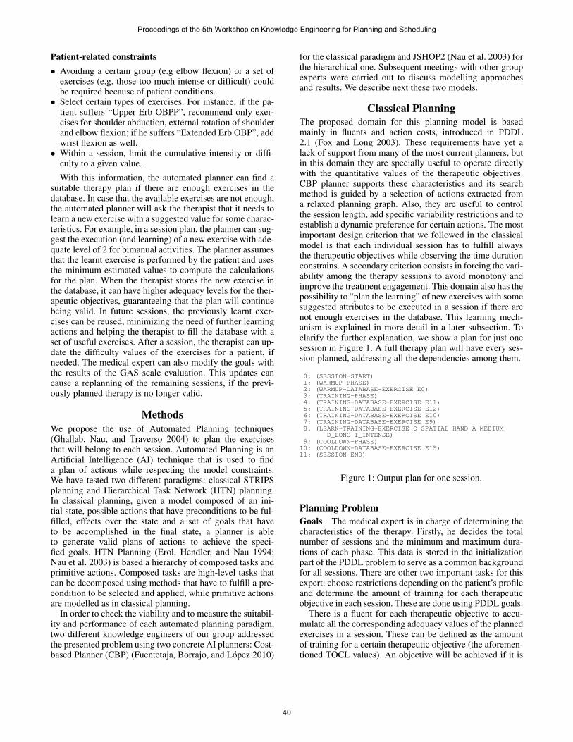
Patient-related constraints• Avoiding a certain group (e.g elbow flexion) or a set of

exercises (e.g. those too much intense or difficult) couldbe required because of patient conditions.

• Select certain types of exercises. For instance, if the pa-tient suffers “Upper Erb OBPP”, recommend only exer-cises for shoulder abduction, external rotation of shoulderand elbow flexion; if he suffers “Extended Erb OBP”, addwrist flexion as well.

• Within a session, limit the cumulative intensity or diffi-culty to a given value.

With this information, the automated planner can find asuitable therapy plan if there are enough exercises in thedatabase. In case that the available exercises are not enough,the automated planner will ask the therapist that it needs tolearn a new exercise with a suggested value for some charac-teristics. For example, in a session plan, the planner can sug-gest the execution (and learning) of a new exercise with ade-quate level of 2 for bimanual activities. The planner assumesthat the learnt exercise is performed by the patient and usesthe minimum estimated values to compute the calculationsfor the plan. When the therapist stores the new exercise inthe database, it can have higher adequacy levels for the ther-apeutic objectives, guaranteeing that the plan will continuebeing valid. In future sessions, the previously learnt exer-cises can be reused, minimizing the need of further learningactions and helping the therapist to fill the database with aset of useful exercises. After a session, the therapist can up-date the difficulty values of the exercises for a patient, ifneeded. The medical expert can also modify the goals withthe results of the GAS scale evaluation. This updates cancause a replanning of the remaining sessions, if the previ-ously planned therapy is no longer valid.

MethodsWe propose the use of Automated Planning techniques(Ghallab, Nau, and Traverso 2004) to plan the exercisesthat will belong to each session. Automated Planning is anArtificial Intelligence (AI) technique that is used to finda plan of actions while respecting the model constraints.We have tested two different paradigms: classical STRIPSplanning and Hierarchical Task Network (HTN) planning.In classical planning, given a model composed of an ini-tial state, possible actions that have preconditions to be ful-filled, effects over the state and a set of goals that haveto be accomplished in the final state, a planner is ableto generate valid plans of actions to achieve the speci-fied goals. HTN Planning (Erol, Hendler, and Nau 1994;Nau et al. 2003) is based a hierarchy of composed tasks andprimitive actions. Composed tasks are high-level tasks thatcan be decomposed using methods that have to fulfill a pre-condition to be selected and applied, while primitive actionsare modelled as in classical planning.

In order to check the viability and to measure the suitabil-ity and performance of each automated planning paradigm,two different knowledge engineers of our group addressedthe presented problem using two concrete AI planners: Cost-based Planner (CBP) (Fuentetaja, Borrajo, and Lopez 2010)

for the classical paradigm and JSHOP2 (Nau et al. 2003) forthe hierarchical one. Subsequent meetings with other groupexperts were carried out to discuss modelling approachesand results. We describe next these two models.

Classical PlanningThe proposed domain for this planning model is basedmainly in fluents and action costs, introduced in PDDL2.1 (Fox and Long 2003). These requirements have yet alack of support from many of the most current planners, butin this domain they are specially useful to operate directlywith the quantitative values of the therapeutic objectives.CBP planner supports these characteristics and its searchmethod is guided by a selection of actions extracted froma relaxed planning graph. Also, they are useful to controlthe session length, add specific variability restrictions and toestablish a dynamic preference for certain actions. The mostimportant design criterion that we followed in the classicalmodel is that each individual session has to fulfill alwaysthe therapeutic objectives while observing the time durationconstrains. A secondary criterion consists in forcing the vari-ability among the therapy sessions to avoid monotony andimprove the treatment engagement. This domain also has thepossibility to “plan the learning” of new exercises with somesuggested attributes to be executed in a session if there arenot enough exercises in the database. This learning mech-anism is explained in more detail in a later subsection. Toclarify the further explanation, we show a plan for just onesession in Figure 1. A full therapy plan will have every ses-sion planned, addressing all the dependencies among them.

0: (SESSION-START)1: (WARMUP-PHASE)2: (WARMUP-DATABASE-EXERCISE E0)3: (TRAINING-PHASE)4: (TRAINING-DATABASE-EXERCISE E11)5: (TRAINING-DATABASE-EXERCISE E12)6: (TRAINING-DATABASE-EXERCISE E10)7: (TRAINING-DATABASE-EXERCISE E9)8: (LEARN-TRAINING-EXERCISE O_SPATIAL_HAND A_MEDIUM

D_LONG I_INTENSE)9: (COOLDOWN-PHASE)10: (COOLDOWN-DATABASE-EXERCISE E15)11: (SESSION-END)

Figure 1: Output plan for one session.

Planning ProblemGoals The medical expert is in charge of determining thecharacteristics of the therapy. Firstly, he decides the totalnumber of sessions and the minimum and maximum dura-tions of each phase. This data is stored in the initializationpart of the PDDL problem to serve as a common backgroundfor all sessions. There are other two important tasks for thisexpert: choose restrictions depending on the patient’s profileand determine the amount of training for each therapeuticobjective in each session. These are done using PDDL goals.

There is a fluent for each therapeutic objective to accu-mulate all the corresponding adequacy values of the plannedexercises in a session. These can be defined as the amountof training for a certain therapeutic objective (the aforemen-tioned TOCL values). An objective will be achieved if it is


40

trained enough, so it is sufficient to assign a goal with alower threshold for each objective to be trained. As an ex-ample, for a 30 minutes session:(>= (TOCL t_bimanual) 15)(>= (TOCL t_unimanual_fine) 7)(>= (TOCL t_spatial_arm) 7)

Numeric goals in PDDL permit a great flexibility to con-figure the range of desired values for each fluent at the endof each session. It could be also possible to establish an up-per limit for each objective (less or equal condition) or evenavoid the training of a certain objective (equals to zero), butthis has less medical sense because these values are just aform to represent the priority of the therapeutic objectivesand they do not need to be directly related with the intensityof the exercises, for which there is a different fluent.

Exercise Database The database contains all the storedexercises. It is fully managed by the therapist, adding ex-ercises when the system suggests it with learning actions orwhen the therapist finds it convenient. This information ob-serves all the characteristics of the exercises mentioned inprevious sections. The difficulty value of each exercise isstored in the patient’s profile, but to simplify we considerthat they are loaded in the PDDL problem file before theplanning task. To assure the variability constraints, there aretwo additional fluents representing the session number andthe position of the exercise in the the last session where itappeared. Each exercise has a predicate to be able to appearin the warm-up, training or cool-down phase.

The system assumes that the information of the databaseis coherent, so the therapist has to be sure that the exercisesare correct when he adds them. For example, warm-up ex-ercises should not be too intense. With these considerations,the session plan will start with soft intensity, followed byan intense training phase and ending with softer exercisesagain. Below there is an example of a generic therapeuticexercise (e7) modelled in PDDL:(e_phase e7 p_training)(e_group e7 g_arm_independence)(= (e_last_session e7) 2)(= (e_last_position e7) 4)(= (e_intensity e7) 48)(= (e_difficulty e7) 39)(= (e_duration e7) 4)(= (e_adequacy e7 t_bimanual) 0)(= (e_adequacy e7 t_unimanual_fine) 3)(= (e_adequacy e7 t_unimanual_coarse) 0)(= (e_adequacy e7 t_spatial_arm) 1)(= (e_adequacy e7 t_spatial_hand) 0)

Planning DomainActions All actions are strongly based in fluents, havingnumeric preconditions and action costs. There are two stan-dard action types: to control the session flow and to add ex-ercises from the database.

Flow control actions allow moving among warming up,training and cooling down phases or determining the startand end of a session. When the minimum time for a phasehas been reached, it is possible to move to the next phase orto finish the session.

The basic way to add exercises to a session is through ac-tions which select them from the database. They check thatthere is available time in the current phase and constraintslike the maximum cumulative intensity. Only exercises for

the current phase can be selected. To assure variability thereare two restrictions modelled as preconditions in the PDDLdomain:

• The exercise cannot be used in the last three sessions.

• In the training phase, an exercise cannot be trained in thesame position as in the last session in which it appeared.2

Learning Exercises Learning actions helps the therapistto add new useful exercises to the database as the systemis being used. When the system has difficulties to find avalid plan, it can ask the therapist to provide a new exerciseto continue planning. Our hypothesis states that the biggerthe database is, the less new learnings will be needed. It ispreferable to use exercises in the database instead of learn-ing new ones, but is not necessary to explore all the possiblecombinations before trying a learning action. This has beencontrolled using a higher action cost. The planner tries tominimize the total cost of the plan, so learning actions tendto be used few times.

To increase variability, the action cost will be higher whenthe new exercise allows reaching the problem goals faster. Inthis way, longer and less adequate exercises are preferred forthe main target.

Planning StrategyClassical planning has to deal with a major problem in thisdomain. Plan only one session is somewhat relatively easy,but a real therapy is composed of about 20 sessions. The firstapproximation was to plan the full therapy, generating planswhich contain more than 250 actions. Planning multiple ses-sions in one run causes a non-linear complexity increase be-cause there are dependencies among them. The planner hasto do backtracking if the selected exercises for a session arenot valid. The problem appears when the planner goes backfurther than needed, maybe many valid sessions, forcing toreplan these sessions again to find a valid alternative for alater one. A smaller backtracking of just a few actions couldsolve the situation allowing reordering of the exercises, se-lecting others or planning the learning of a new one to con-tinue onward.

We use a divide and conquer strategy to plan each sessionindividually taking into account the dependencies of one an-other. In particular, the planner is called one time for eachsession that we want to plan. Each time that the planner re-turns a plan, it is parsed to determine all the database andlearnt exercises planned. For the next session, a new prob-lem file is generated to update the predicates and functionsof the exercises of the last session planned, and add the newlearnt exercises to the database. Then, the planner is exe-cuted again with the problem file for the next session. So foreach session, a PDDL problem file is generated with the newexercises and updates of the database exercises. The exper-iments showed that this strategy is much faster than plan-ning all the sessions in one run, without affecting the quality

2For warm-up and cool-down phases the condition is not appli-cable because a long exercise can reach by itself the minimum timeof the phase and cannot be reordered (e.g. in the warm-up phase,such exercise will always appear in the first position).


41

1 2 3 4 5 6 7 81 e0 e9 e11 e12 e10 e7 e15

2 e4 e2 e5 e6 L L L e13

3 e1 e3 e8 L L L L e16

4 L L L L L L e17

5 e0 e11 e12 e10 e9 L e15

6 e4 e2 e6 L19 e7 e5 L20 e13

7 e1 e3 L24 e8 L23 L22 e16

8 L25 L26 L30 L27 L28 L29 e17

9 e0 e12 e10 L31 e11 e9 e1510 e4 e2 L19 L20 e6 e7 e13

11 e1 e3 L22 L23 L24 e8 e16

12 L L25 L26 L29 L30 L27 L28 e17

13 e0 e10 L21 e12 e9 e11 e15

14 e4 e2 e7 e6 L20 L19 e13

15 e1 e3 L24 e8 L22 L23 e16

16 L25 L27 L31 L26 e5 L29 L30 e17

17 e0 e11 e12 L28 e10 e9 e15

18 L32 e4 e2 L19 e6 L20 e7 e13

19 e1 e3 L22 L23 L24 e8 e16

20 L25 L26 e5 L29 L30 e17

Sessions

Planned exercises

Table 1: Therapy plan with few exercises in the database.An “e” or “L” with a number represents an exercise storedin the database (initial or learnt, respectively). A single “L”represents the learning and execution of a new exercise.

of the plans. The capacity to learn new exercises gives tothe sessions some locality properties that can be exploited toavoid time-consuming backtracking among sessions.

Empirical EvaluationWe used the CBP automated planner (Fuentetaja, Borrajo,and Lopez 2010) because it was specially designed to workwith action costs, so its heuristics reduce the total number ofnew learned actions. In Table 1 there is an example of a ther-apy with 20 sessions. The database starts with a controlledset of exercises: 5 warm-up, 8 training and 5 cool-down ex-ercises.

In session 1, the planner only uses exercises from thedatabase because they are useful to reach the TOCL thresh-olds. In sessions 2 and 3, it needs to learn due to variabilityconstraints. In session 4, almost all the exercises has beenused in the last three sessions, so it has to continue learningnew ones. In session 5, the planner can use the set of exer-cises of session 1 again, but it varies the order of the trainingphase because the exercises cannot appear in the same posi-tion as the last time. In the following sessions, the learnt ex-ercises are reused because they continue being useful to ful-fill the goals, so more learning actions are not needed. Notethat the planned sessions are very different among them.

The new learnings in session 5 and 12 show that learn-ing actions are not completely prohibited, so it is not neededto explore all the combinations in the database before usinga learning action. Also, we only use the first plan returnedby CBP. This planner can improve the plans iteratively if ithas time, but the first plan returned is good enough to seehow the system works. With this configuration, the planning

time usually does not take more than five minutes. In the ini-tial experimentation, we observed that the principal aspectsthat increase planning time are the number of learned actionsneeded and the TOCL thresholds.

HTN PlanningThe automatic generation of therapies is a problem that canalso be managed in a hierarchical way, where the top ofthe pyramid contains a task representing the whole therapy,which is divided into sessions and each session comprises aset of exercises, as shown in Figure 2. The session structureis given by the hierarchical and order relationships repre-sented in the HTN decomposition. This approach aims toprovide an easily extendible and configurable model, wherehuman expert knowledge can be included at any time.

generate-therapy

generate-session new therapy

new session

finish therapy

finish session generate-exercises

fill-warmup-exercises fill-training-exercises fill-cooldown-exercises

add

exercise learn

exercise

add exercise

learn exercise

add

exercise learn

exercise

Figure 2: Hierarchical Task Network model schema.

Planning ProblemGoals As shown in Figure 2, the goal of the HierarchicalTask Network is the root level of the tree (generate-therapy).This general task comprises three arguments: number of ses-sions to plan, duration interval for each session and patientidentifier. This task can be refined using the HTN decompo-sition methods until a set of primitive actions completes theplan, which should reach the TOCLs. These TOCLs are alsomodelled as numeric predicates in the problem description.Furthermore, with the aim to parametrize the search (timeand possible exercises in a phase or session), a set of predi-cates is also included.

Exercise Database The exercise database has been mod-elled similarly to how it has been described for the classicalplanning approach. The only difference is purely technicaldue to the representation language of the HTN planner usedfor evaluation, described later.

Planning DomainThe HTN planning domain is organized as shown in Fig-ure 2, where a set of exercises is generated for a numberof sessions. This behaviour is modelled as a recursive task


42

(generate-session) which receives the current session num-ber and the total number of sessions as parameters. This cur-rent session number (?csn) is used as identifier by the plan-ning domain and increased to generate new sessions.(:method (generate-session ?csn ?tsn);main((call <= ?csn ?tsn))

((!new-session ?csn ?tsn)(generate-exercises ?csn)(generate-session (call + ?csn 1) ?tsn))

;stop((call > ?csn ?tsn))

nil)

Each session is divided into three phases modelled aslower-level tasks: warm-up phase, training phase and cool-down phase. The system must distinguish which exercisesare appropriate for each phase depending on its features, anddecides if learning a new exercise is required during plan-ning time.

Axioms Axioms allow to infer new predicates from theevaluation of a logical expression (abductive inference).We have defined axioms to control the time intervals ofphases and to manage which exercises are more appropri-ate for that phase according to the parameters specified inthe planning problem. For example, (cooldown-time) and(cooldown-exercise) in Figure 3 are calls to axioms.

Each session begins and ends with less intense and dif-ficult exercises and the middle of the session consists ofgreater intensity and difficulty exercises. The expectationfor each session (comprising three phases) is that the valuesof intensity and difficulty follow a Gaussian distribution, asshown later in the empirical evaluation (see Figure 4). Us-ing axioms throughout the planning domain simplifies themodelling process of this requirement.

Tasks and Methods Methods are used to refine compoundtasks into lower-level tasks or primitive actions. These meth-ods have a precondition that needs to be fulfilled in order tobe applied. In our model, we have used five tasks:

1. (generate-therapy) has a unique method with empty pre-condition that uses a total-order decomposition to call thelower-level task (generate-session).

2. (generate-session) is modelled as a recursive task that hasa method to call lower-level task (generate-exercises) anda “nil” method that stops when the number of sessionsrequired is reached.

3. (generate-exercises) has a unique method with empty pre-condition that calls a total-ordered sequence of lower-level tasks (one for each phase).

4. (fill-phase-exercises) are modelled with three methods.The first one checks a) that the current time is withinthe phase time interval, b) that the exercise is suitable forthe phase and c) that the exercise selected has not beenalready included in the ongoing generated session plan.Figure 3 shows a high-level description of how the (fill-cooldown-exercises) task has been modelled. The firstmethod uses a “sort-by” function that drives the plannerin the order in which the variable bindings will be evalu-ated for the method precondition. This “sort-by” functioncalculates an heuristic value (?ht), modelled as follows:

htex =

nobjectives∑i=1

(1

di2 + 1

− extimes used

numsessions) (1)

where di, for each therapeutic objective i, is the distance(a minus operation) between the current cumulative level(if the exercise would be included) to the desired TOCLfor the planned session. So, the function rewards exerciseswhose contribution minimizes the distance to the frontiersolution. The last part of the equation penalizes the num-ber of times an exercise has been previously used.The second method is applied when all the possible exer-cises have been already included in a session, so there isno available exercises to add. In this case a new exerciseneeds to be acquired (“learn” action) from the therapist.Exercises will be added taking into account the heuris-tic and recursive calls to (fill-cooldown-exercises) and itwill be carried out till the preconditions fails. In this lastcase, the third method precondition is evaluated (TOCLreached within the maximum session time specified); if itis fulfilled, the plan is valid. Otherwise the planner will dobacktracking to check other exercise sets, until this condi-tion is reached.

Primitive Actions We use dummy actions to delimit startand end of sessions and therapy (see Figure 2). The action toadd an exercise updates the current session time (adding theexercise duration) and the current cumulative level for thetherapeutic objectives in that session. It also updates the sta-tus of the exercise to “used” and the counter of times used.At the time of writing this paper, the “learn” action estab-lishes fixed values for the exercise attributes. Improving thisbehaviour is subject of future work.

;; Receives the session number

(:method (fill-cooldown-exercises ?csn)

(:sort-by ?ht >

((e-target1 ?e ?et1)

(current-acc t1 ?csn ?ct1a)

(baseline t1 ?t1bl)

...

(assign ?d1 (call - ?t1bl (call + ?et1 ?ct1a)))

...

(assign ?h1 (call / 1 (call + (call * ?d1 ?d1) 1)))

...

(e-used ?e ?n-used) (t-session-number ?tsn)

(assign ?ht (call - (call + ?h1 ... ?h5) (call / ?n-used ?tsn)))

...

(cooldown-time ?cst ?minST ?maxST)

(cooldown-exercise ?e ?minST ?maxST)

(not (used ?e ?csn))))

((!add-ex ?e cool-down)

(fill-cooldown-exercises ?csn))

(forall (?e) ((exercise ?e)) (used ?e ?csn))

((!learn))

((current-session-time ?csn ?cst)

(session-max-time ?csn ?maxST)

(call <= ?cst ?maxST)

(current-acc t1 ?csn ?ct1a) (TOCL t1 ?t1bl) (call >= ?ct1a ?t1bl)

...

((!finish-session ?csn)))

Precondition 1

Actions and task calls

Precondition 3


2

Met

hod

1 M

etho

d 3

Task definition

Met

hod

2


Precondition 2

Figure 3: JSHOP2 code for the task to include a set of exer-cises in the cool-down phase of a session.


43

Planning StrategyOur hypothesis states that a well modelled hierarchical rep-resentation of the domain knowledge, along with parametersto drive the search appropriately, could generate successfulsolutions with a improved quality. In other words, we lookfor a parametrized design to provide a flexible configura-tion to the physicians. Moreover, in order to reflect the med-ical criteria in the resulting plan, the heuristic function is incharge of the exercises selection. As explained before, thisfunction is also used to penalize the most repetitive exercisesreducing the heuristic value, but this does not avoid the oc-currence of the same exercise throughout sessions. That iswhy we consider the variability as soft constraint.

The HTN approach can search towards reaching generaltherapeutic objectives that imply interactions among ses-sions. These interactions can occur due to a) the exercisedistribution of previous ongoing planned sessions that couldaffect to future ones, b) the TOCLs of subsequent sessionscan be updated by the plan of earlier sessions and c) chas-ing possible distributions (eg. time, intensity, TOCLs) forthe whole therapy predefined by physicians. This is the mo-tivation to propose a recursive model in order to generatemultiple sessions. The HTN approach preserves the capabil-ity of backtracking through past sessions without mediationof an external program.

Empirical EvaluationWe have used the SHOP2 HTN language (Nau et al. 2003)for modelling the planning domain and JSHOP23 to test theplan generation. The SHOP2 language is provided with agreat expressiveness that allows axiomatic inference, sym-bolic and numerical computation, call to external programsand use of conditional quantifiers, to name some features.

In order to evaluate the behaviour of the hierarchical do-main, a set of 72 exercises are included in the planning prob-lem. This experiment has been carried out with the follow-ing configuration: 30 sessions to generate, 25-30 minutes persession, 20% of the total session time is assigned to eachwarm-up and cool-down phases and the remainder 60% isfor training phase. The established intervals to consider anexercise as a candidate for each phase are: warm-up intensity[0-30], warm-up difficulty [0-20], training intensity [30-50],training difficulty [30-50], cool-down intensity [0-20] andcool-down difficulty [0-30]. It is assumed that an exercisecould be considered as warm-up and cool-down according totheir values. The effects of the exercise distribution is shownin Figure 4, where an approximate Gaussian distribution ofthe intensity and difficulty within the phases is achieved.

Discussion and ConclusionsTo conclude this manuscript we have created a qualitativecomparison of the two approaches that highlight the maintopics addressed. Table 2 represents a summary of this com-parison. Some further take-home messages are describednext. Firstly, this work provides an original model based onnumeric values of a new kind of problem which is useful

3It uses a planning compilation technique to synthesize domain-dependent planners from SHOP2 domain descriptions.

0

10

20

30

40

50

1 2 3 4 5 6 7 8 9 10 11Average Exercise Set (for 30 sessions)

IntensityDifficulty

Figure 4: Represents the average values of the intensityand difficulty for 30 generated sessions. Along the differ-ent phases (warm-up, training and cool-down), the achievedprogress is represented by these Gaussian distributions.

to compare capabilities and behaviour among different au-tomated planners. Secondly, we think that more flexibilityfor the user seems to be available in the HTN model, wheremore complex expert knowledge could be represented eas-ily, however costs and preferences used in classical planningare very suitable for this problem. Third, with regard to howto achieve variability while trying to fulfil our requirements,we noted that the sort-by function used in JSHOP2 needs toarrange and order many bindings before the task decomposi-tion is applied, which may affect its performance. This couldpossibly be improved by modelling the heuristic functionusing a java comparator function, as offered by JSHOP2.Fourth, the divide and conquer strategy used in the classi-cal approach eliminates the backtracking to previous ses-sions to improve the planning time. On the other hand, theHTN model can generate plans using backtracking amongsessions to solve their interactions. Finally, CBP does notuse heuristics for fluents, which could be very helpful forthis domain to reduce the planning time. OPTIC (Benton,Coles, and Coles 2012) provides this kind of heuristics, soit could be a future option to explore. With regard to tem-poral constraints, if more complex ones would be needed,the temporal representation provided by PDDL2.1 could behandled through planners like OPTIC (Benton, Coles, andColes 2012) or the HTN planner SIADEX (Castillo et al.2006). In the case of HTN, it would be interesting to explorenew preference-based planning approaches.

To sum up, we have presented two ways to reach plansdriven by general therapeutic objectives modelled numeri-cally. We plan to do a better quantitative comparison in termsof performance, addressing the issues previously discussed.

AcknowledgementsThis work has been partially granted by the Spanish Ministe-rio de Economıa y Competitividad (MINECO) funds undercoordinated project no. TIN2012-38079-C03-01, TIN2012-38079-C03-02 and TIN2012-38079-C03-03, and FEDERINNTERCONECTA ADAPTA 2012. We also are gratefulto the medical team of the Virgen del Rocıo University Hos-pital for their participation.


44

Constraints, Requirements Classical Planning HTN PlanningAssuring Variability

• Avoids repeating exercises in the same session.• Avoids repeating an exercise in the last three sessions.• In the training phase, an exercise cannot be planned in the same

position than in the last occurrence.

• Avoids repeating exercises in the same session.• Heuristic sort-by function penalized for exercises that occur re-

peatedly.

Phase Selection PDDL predicate relating each exercise to its corresponding phase. Axioms limiting the exercise selection whose minimum and maxi-mum duration, intensity and difficulty can be defined by physiciansfor each phase.

Phase Time Intervals It is parametrized through the minimum and maximum duration foreach phase, which is assigned by the medical expert.

Time is parametrized through axioms according to accumulatedpercentage of total time for each phase (eg. 0.2, 0.7, 1.0).

Learning new exercise Suggests which attribute values should have a new learnt exercise,preferring exercises which can improve the session variability.

It does not suggest the minimum values yet, but it is already mod-elled as a new HTN method that can add new exercises during plan-ning time.

Achieving Goals• The automated planner has to achieve the TOCL thresholds

which are the goals established in the planning problem, whileobserving all the constraints set by the physician.

• Minimizes the total cost of the plan, where learning a new exer-cise has more cost than use one from the database.

• Total-order hierarchical network expressing the three phases.TOCLs and expected session time should be reached, otherwisebacktracking occurs to find a suitable exercise set.

• Driving exercise selection through a sort-by function (see de-scription above).

Planning Multiple Sessions Divide and conquer strategy which calls the planner one time persession, improving planification time without affecting the qualityof the plan thanks to the learning actions.

HTN Planning is done as usual in one run, doing backtracking whenexercise sets dont reach expected goals.

Table 2: Qualitative comparison of Classical and HTN approaches for the presented problem.

ReferencesAhmed, S.; Gozbasi, O.; Savelsbergh, M. W. P.; Crocker, I.;Fox, T.; and Schreibmann, E. 2010. An automated intensity-modulated radiation therapy planning system. INFORMSJournal on Computing 22(4):568–583.Benton, J.; Coles, A. J.; and Coles, A. I. 2012. Tempo-ral planning with preferences and time-dependent continu-ous costs. In Proceedings of the Twenty Second Interna-tional Conference on Automated Planning and Scheduling(ICAPS-12).Calderita, L.; Bustos, P.; Suarez Mejias, C.; Fernandez, F.;and Bandera, A. 2013. Therapist: Towards an autonomoussocially interactive robot for motor and neurorehabilitationtherapies for children. In 7th International Conference onPervasiveHealth, 374–377.Castillo, L. A.; Fernandez-Olivares, J.; Garcia-Perez, O.;and Palao, F. 2006. Efficiently handling temporal knowl-edge in an htn planner. In ICAPS, 63–72.Erol, K.; Hendler, J.; and Nau, D. S. 1994. HTN planning:Complexity and expressivity. In AAAI, volume 94, 1123–1128.Fdez-Olivares, J.; Castillo, L. A.; Cozar, J. A.; and Garcıa-Perez, O. 2011. Supporting clinical processes and decisionsby hierarchical planning and scheduling. Computational In-telligence 27(1):103–122.Fox, M., and Long, D. 2003. PDDL2.1: An extension toPDDL for expressing temporal planning domains. J. Artif.Intell. Res.(JAIR) 20:61–124.Fuentetaja, R.; Borrajo, D.; and Lopez, C. L. 2010. A look-

ahead B&B search for cost-based planning. In Current Top-ics in Artificial Intelligence. Springer. 201–211.Ghallab, M.; Nau, D.; and Traverso, P. 2004. Automatedplanning: theory & practice. Elsevier.Gonzalez-Ferrer, A.; Ten Teije, A.; Fdez-Olivares, J.; andMilian, K. 2013. Automated generation of patient-tailored electronic care pathways by translating computer-interpretable guidelines into hierarchical task networks. Ar-tificial Intelligence in Medicine 57(2):91–109.Morignot, P.; Soury, M.; Leroux, C.; Vorobieva, H.; andHede, P. 2010. Generating scenarios for a mobile robotwith an arm: Case study: Assistance for handicapped per-sons. In Proceedings of 11th International Conference onControl Automation Robotics & Vision, 976–981. IEEE.Nau, D. S.; Au, T.-C.; Ilghami, O.; Kuter, U.; Murdock,J. W.; Wu, D.; and Yaman, F. 2003. SHOP2: An HTN plan-ning system. J. Artif. Intell. Res.(JAIR) 20:379–404.Peleg, M. 2013. Computer-interpretable clinical guidelines:A methodological review. Journal of Biomedical Informat-ics 46(4):744–763.Schimmelpfeng, K.; Helber, S.; and Kasper, S. 2012. Deci-sion support for rehabilitation hospital scheduling. OR spec-trum 34(2):461–489.Turner-Stokes, L. 2009. Goal attainment scaling (GAS)in rehabilitation: a practical guide. Clinical rehabilitation23(4):362–70.


45

Knowledge Engineering for Planning-Based Hypothesis Generation

Shirin Sohrabi Octavian Udrea Anton V. RiabovIBM T.J. Watson Research Center

PO Box 704, Yorktown Heights, NY 10598, USA{ssohrab, oudrea, riabov}@us.ibm.com

Abstract

In this paper, we address the knowledge engineering prob-lems for hypothesis generation motivated by applications thatrequire timely exploration of hypotheses under unreliable ob-servations. We looked at two applications: malware detectionand intensive care delivery. In intensive care, the goal is togenerate plausible hypotheses about the condition of the pa-tient from clinical observations and further refine these hy-potheses to create a recovery plan for the patient. Similarly,preventing malware spread within a corporate network in-volves generating hypotheses from network traffic data andselecting preventive actions. To this end, building on the al-ready established characterization and use of AI planning forsimilar problems, we propose use of planning for the hypoth-esis generation problem. However, to deal with uncertainty,incomplete model description and unreliable observations,we need to use a planner capable of generating multiple high-quality plans. To capture the model description we propose alanguage called LTS++ and a web-based tool that enables thespecification of the LTS++ model and a set of observations.We also proposed a 9-step process that helps provide guid-ance to the domain expert in specifying the LTS++ model.The hypotheses are then generated by running a planner onthe translated LTS++ model and the provided trace. The hy-potheses can be visualized and shown to the analyst or can befurther investigated automatically.

IntroductionSeveral application scenarios require the construction of hy-potheses presenting alternative explanation of a sequence ofpossibly unreliable observations. For example, the evolutionof the state of the patient over time in an Intensive Care Unit(ICU) of a hospital can be inferred from a variety of mea-surements. Similarly, observations from network traffic canindicate possible malware. The hypotheses, represented asa sequence of changes in patient state, aim to present anexplanation for these observations, while providing deeperinsight into the actual underlying causes for these observa-tions, helping to make decisions about further testing, treat-ment or other actions.

Expert judgment is the primary method used for generat-ing hypotheses and evaluating their plausibility. Automatedmethods have been proposed, to assist the expert, and helpimprove accuracy and scalability. Notably, model-based di-agnosis methods can determine whether observations can be

explained by a model (e.g., (Cassandras and Lafortune 1999;Sampath et al. 1995)). Recently, several researchers haveproposed use of automated planning technology to addressseveral related class of problems including diagnosis (e.g.,(Sohrabi, Baier, and McIlraith 2010; Haslum and Grastien2011)), plan recognition (Ramırez and Geffner 2009), andfinding excuses (Gobelbecker et al. 2010). These problemsshare a common goal of finding a sequence of actions thatcan explain the set of observations given the model-baseddescription of the system. However, most of the existing lit-erature make an assumption that the observations are all per-fectly reliable and should be explainable by the system de-scription, otherwise no solution exists for the given problem.But that is not true in general. For example, even though ob-servations resulting from the analysis of network data canbe unreliable, we would still like to explain as many obser-vations as possible with respect to our model; as a furthercomplication, we cannot assume the model is complete.

In 2011, Sohrabi et al. established a relationship betweengenerating explanations, a more general form of diagno-sis, and a planning problem (Sohrabi, Baier, and McIlraith2011). Recently, we extend this work to address unreliableobservations and showed how to generate multiple high-quality plans or the plausible hypotheses. (Sohrabi, Udrea,and Riabov 2013)1. In this paper, we address knowledge en-gineering problems of capturing the domain knowledge.

To capture the model description we propose a languagecalled LTS++, derived from LTS (Labeled Transition Sys-tem) (Magee and Kramer 2006) for defining models forhypothesis generation, and associating observation types.LTS++ is less expressive than the general Planning DomainDefinition Language (PDDL) specification of a planningproblem (McDermott 1998). However, in our experience,the domain expert finds writing an LTS++ language muchsimpler than PDDL. To further help the domain expert, wealso proposed a process that helps provide guidance in spec-ifying the LTS++ model. Additionally, we developed a web-based tool that enables the specification of the LTS++ modeland a set of observations. Our tool features syntax highlight-ing, error detection, and visualization of the state transition

1We include the description of our approach to hypothesis gen-eration from that prior work, but LTS++ and our tools for knowl-edge engineering have not been previously described.


46

Infec&on(

ByEmail( ByNeighbor(ByDownload(

CC_Rendezvous(ByDomainName( ByIRC( ByNeighbor( ByP2P(

Exploit(

ClickFraud(

DataExfil( DDoS(

FastFlux(

Spam(

Crawling(PortScanned(

Executable|BlacklistedDomain(

BlacklistedDomain|HighNXVolume|LowPopularityDomain(

IncreasedIRC( ConnectedToInfected( IPwoDNS( IncreasedAdTraffic(

HighSessionLen|(HighSessionBytes(

ManyReqToDomain(

DNSRegistra&ons(

IncreasedOutEmail|(EmailUnknownDest(

Executable|BlacklistedDomain|HighNXVolume|LowPopularityDomain(|IncreasedAdTraffic|(HighSessionBytes|HighSessionLen(

Highrisk( Icudeath(

Discharged( Pa2entNoLead(

Infec2on(

Infarc2on(

DCI(

Lowrisk(

Unadmi<ed(

HRVL|LabTestBacteria+|SIRS3|SIRS4(HH1|HH2|An2bioAdmin|SIRS0|SIRS1(

Pa2entLeK(

AngiogramDCI+|CTScanDCI+|HRVL|ClinicalObs+(

AngiogramInfarct+(|CTScanInfarct+(|PupilDilated(

FlatVitals(

HRVL|ECGNoisy(

HRVL|SIRS3|SIRS4|LeadFixed|HH2|HH3|HH4|An2bioAdmin(

Figure 1 (a): Malware detection Figure 1 (b): Intensive care

graph. The hypotheses are then generated by running a plan-ner on the translated LTS++ model and the provided obser-vation trace. The hypotheses can be visualized and shown tothe analyst or can be further investigated automatically.

In the rest of the paper, we will first describe our twoapplication examples in detail. We then describe the archi-tecture of our automated hypothesis exploration problemin which hypothesis generation plays a key role. Then wedescribe the relationship between planning and hypothesisgeneration, which facilitates the use of planning technology.We show our initial experimental results in using planning.We then describe our LTS++ language, the creation process,LTS++ IDE, and show several example problems.

Application DescriptionIn this section we introduce two example applications thatillustrate our approach: intensive care delivery and malwaredetection. A key characteristic of these applications is thatthe true state of monitored patients, network hosts, or otherentities, while essential for timely detection and preventionof critical conditions, is not directly observable. Instead, wemust analyze the sequence of available observations to re-construct the state. To make this possible, our approach re-lies on a model of the entity consisting of states, transitionsbetween states, and many-to-many correspondence betweenstates and observations. In the following sections we willdescribe how these models can be created by the domain ex-perts and encoded in our LTS++ language.

Figure 1 shows state transition systems of intensive caseand malware detection. The rounded rectangles are states.The states are associated with a type, good or bad, and drawnin blue or red respectively. The callouts are observations as-sociated with these states. Note that the observations are ob-tained by analyzing raw data gathered through sensors.

In Figure 1 (a), the bad state correspond to malware life-cycle, such as the host becoming infected with malware, thebot’s rendezvous with a Command and Control (C&C) ma-chine (botmaster), and a number of exploits – uses of thebot for malicious activity. Each of the states can be achievedin many ways, depending on the type and capabilities ofthe malware. For example, the CC Rendezvous state can beachieved by attempting to contact an Internet domain, orvia Internet Relay Chat (IRC) on a dedicated channel. Thegood state in Figure 1 (a) corresponds to a “normal” life-cycle of a web crawler compressed into a single state. Notethat crawler behavior can also generate a subset of the ob-

servations that malware may generate. The callouts are theobservations associated with states. For example, the ob-servation HighNXVolume is an observation associated withthe ByDomainName state that corresponds to an abnormallyhigh number of domain does not exist responses for DomainName System (DNS) queries; such an observation may indi-cate that the bot and its botmaster are using a domain namegeneration algorithm, and the bot is testing generated do-main names trying to find its master.

In Figure 1 (b), the bad states correspond to critical statesof a patient such as Infection, DCI, or Highrisk. The goodstates are the non-critical states. Upon admission the pa-tient is either in Lowrisk or in Highrisk. From a Highriskstate, they may get to the Infection, Infarction, or the DCIstate. From Lowrisk they may get to the Highrisk state orbe Discharged from ICU. The patient enters Icudeath fromInfection, Infarction, or DCI state. The patient’s conditionmay improve; hence the patient’s state may move back tothe Lowrisk state from for example the Infection state. Theobservations are measured based on the raw data capturedby patient monitoring devices (e.g., the patient’s blood pres-sure, heat rate, temperature) as well as other measurementsand computations provided by doctors and nurses. For ex-ample, given the patient’s heart rate, their blood pressure,and their temperature, which are measured continuously,their SIRS score can be computed, producing an integer be-tween 0 to 4. Similarly, a result of CT Scan, or a lab test willindicate other possible observations about the patient.

While the complexity of the analysis involved to obtainone observation can vary, it is important to note that obser-vations are by nature unreliable:

The set of observations will be incomplete. Operationalconstraints will prevent us running in-depth analysis on allof the data all the time. However, all observations are typi-cally time stamped, and hence totally ordered.

Observations may be ambiguous. This is depicted in Fig-ure 1, where for instance contacting a blacklisted domainmay be evidence of malware activity, or maybe a crawlerthat reaches such a domain during normal navigation. Simi-larly, Heart Rate Variability Low (HRVL) may be explainedby many states such as DCI or Highrisk or Infection.

Not all observations will be explainable. There are severalreasons while some observations may remain unexplained:(i) observations are (sometimes weak) indicators of a behav-ior, rather than authoritative measurements; (ii) the modeldescription is by necessity incomplete, unless we are able to


47

design a perfect model; (iii) in the case of malware detec-tion, malware could try to confuse detectors by either hidingin normal traffic patterns or originating extra traffic.

For Figure 1 (a) one can consider the following two ob-servations for a host: (o1) a download from a blacklisted do-main and (o2) an increase in traffic with ad servers. Notethat according to Figure 1 (a), this sequence could be ex-plained by two hypotheses: (a) a crawler or (b) infection bydownloading from a blacklisted domain, a C&C rendezvouswhich we were unable to observe, and an exploit involv-ing click fraud. In such a setting, it is normal to believe (a)is more plausible than (b) since we have no evidence of aC&C rendezvous taking place. However, take the sequence(o1) followed by (o3) an increase in IRC traffic followed by(o2). In this case, it is reasonable to believe that the pres-ence of malware – as indicated by the C&C rendezvous onIRC – is more likely than crawling, since crawlers do notuse IRC. The crawling hypothesis cannot be completely dis-carded since it may well be that a crawler program is runningin background, while a human user is using IRC to chat.

Consider the following observation sequence for themodel in Figure 1 (b): HH3, HRVL. This denotes a patientwith a Hunt and Hess (a grading system used to classify theseverity of subarachnoid hemorrhage) score of 3, followedby HRVL. Since HRVL is an ambiguous observation – i.e.,can be indicative of multiple states –, equally plausible hy-potheses may be:

Unadmitted→ Highrisk orUnadmitted→ Highrisk→ PatientNoLead orUnadmitted→ Highrisk→ Infarction orUnadmitted→ Highrisk→ DCI.

Note, although the current state of the patient is unknown,the generated hypotheses indicate that it is one of Highrisk,PatientNoLead, Infarction or DCI.

Given a sequence of observations and the model, the hy-pothesis generation task infers a number of plausible hy-potheses about the evolution of the entity. Practically, wehave to analyze multiple hypotheses about an entity becausethe state transition model may be incomplete or the obser-vations may be unreliable. The result of our automated tech-nique can then be presented to a network administrator (or toa doctor) or to an automated system for further investigationand testing. Next, we will describe briefly all the necessarycomponents for hypothesis exploration.

ArchitectureOur work on automated exploration of hypotheses focuseson the Hypothesis Generation, which is part of a larger auto-mated data analysis system that includes sensors, actuators,multiple analytic platforms and a Tactical Planner. TacticalPlanner, for the purpose of this paper, should be viewed as acomponent responsible for execution of certain strategic ac-tions and it can be implemented using, for example, a clas-sical planner to compose analytics (Bouillet et al. 2009). Ahigh-level overview of the complete system architecture isshown in Figure 2. All components of the architecture, withthe exception of application-specific analytics, sensors, andactuators, are designed to be reused without modification ina variety of application domains.

Analytic Platform(s)

Sensors Actuators

Offline Analytics

Strategic Planner

Hypothesis Generator Tactical Planner

Online Analytics

Entities

World

Data Store

Figure 2: System architecture

The system receives input from Sensors, and Analyticstranslate sensor data to observations. The Hypothesis Gen-erator interprets the observations received from analytics,and generates hypotheses about the state of Entities in theWorld. Depending on application domain, the entities maycorrespond to patients in a hospital, or to computers con-nected to a corporate network, or other kinds of objects ofinterest. The Strategic Planner evaluates these hypothesesand initiates preventive or testing actions in response. Someof the testing actions can be implemented as additional pro-cessing of data, setting new goals for the Tactical Planner,which composes and deploys analytics across multiple Ana-lytic Platforms. A Hadoop cluster, for example, can be usedas an analytic platform for offline analysis of historical dataaccumulated in one or more Data Stores. Alternatively, aStream Computing cluster can be used for fast online analy-sis of new data received from the sensors.

Preventive actions, as well as some of the testing actions,are dispatched to Actuators. There is no expectation that ev-ery actuation request will succeed, or always happen instan-taneously. Actuation in a hospital setting can involve dis-patching alerts to doctors, or lab test recommendations.

Hypothesis Generation via PlanningIn this section, we define the hypothesis generation problemand describe its relationship to planning. We also provideexperimental evaluation that supports the premise of usingplanning for generating multiple plausible hypotheses. In thenext section, we will describe how the planning model canbe captured using the LTS++ language which we translate toa planning problem. Our tool, LTS++ hypothesis generator,then uses a planning to compute plausible hypothesis andpresent them to the user.

Following our recent work (Sohrabi, Udrea, and Riabov2013), a dynamical system is defined as Σ = (F,A, I),where F is a finite set of fluent symbols, A is a set of ac-tions with preconditions and effects that describes actionsthat account for the possible transitions of the state of theentity (e.g., patient or host) as well as the discard action thataddresses unreliable observations by allowing observationsto be unexplained, and I is a clause over F that defines theinitial state. The instances of the discard action add tran-sitions to the system that account for leaving an observa-tion unexplained. The added transitions ensure that we tookall observations into account, but an instance of the discard

Hand-crafted 10 states 50 states 100 statesObservations % Solved Time % Solved Time % Solved Time % Solved Time

5 100% 2.49 70% 0.98 80% 5.61 30% 14.2110 100% 2.83 90% 2.04 50% 25.09 30% 52.6320 90% 12.31 70% 24.46 - - - -40 70% 3.92 40% 81.11 - - - -60 60% 6.19 - - - - - -80 50% 8.19 - - - - - -100 60% 11.73 10% 10.87 - - - -120 70% 20.35 20% 15.66 - - - -

Table 1: The percentage of problems where the ground truth was generated, and the average time spent for LAMA.

action for a particular observation o indicates that o is notexplained. Actions can be over both “good” and “bad” be-haviors. This maps to “good” and “bad” states of the entity,different from a system state (i.e., set of fluents over F ).

An observation formula ϕ is a sequence of fluents in F werefer to as trace. Given a trace ϕ, and the system descriptionΣ, a hypothesis α is a sequence of actions in A such that αsatisfies ϕ in the system Σ. We also define a notion of plau-sibility of a hypothesis. Given a set of observations, there aremany possible hypotheses, but some could be stated as moreplausible than others. For example, since observations arenot reliable, the hypothesis α can explain a subset of obser-vations by including instances of the discard action. How-ever, we can indicate that a hypothesis that includes the min-imum number of discard actions is more plausible. In addi-tion, observations can be ambiguous: they can be explainedby instances of “good” actions as well as “bad” actions. Sim-ilar to the diagnosis problem, a more plausible hypothesisideally has the minimum number of “bad” or “faulty” ac-tions. More formally, given a system Σ and two hypothesesα and α′ we assume that we can have a reflexive and transi-tive plausibility relation �, where α � α′ indicates that α isat least as plausible as α′.

The hypothesis generation problem is then defined asP = (F,A′, I, ϕ) where A′ is the set A with the addition ofpositive action costs that accounts for the plausibility rela-tion �. A hypothesis is a plan for P, and the most plausiblehypothesis is the minimum cost plan. That is, if α and α′

are two hypotheses, where α is more plausible than α′, thencost(α) < cost(α′). Therefore, the most plausible hypothe-sis is the minimum cost plan.

While some class of plausibility relation can be ex-pressed as Planning Domain Definition Language (PDDL3)(Gerevini et al. 2009) preferences, cost-based planners are(currently) more advanced than PDDL3-based planners, andso the technique proposed by Keyder and Geffner 2009 canbe used to compile preferences into costs, enabling the useof cost-based planners instead.

Computing Plausible HypothesesTo address uncertainty, the unreliability of observations andincomplete model description, we must generate multiplehigh-quality (or low-cost) plans that correspond to a set ofplausible hypothesis. To this end, we adapt our implemen-tation of hypothesis generation from (Sohrabi, Udrea, andRiabov 2013). We encode the plausibility notion as actionscosts. In particular, we assign a high cost to the discard ac-tion in order to encourage explaining more observations. In

addition, we assign a higher cost to all instances of the ac-tions that represent “bad” behaviors than those that repre-sent “good” behaviors. Furthermore, shorter/simpler plansare assumed to be more plausible. To address observations,we similarly compile them away in our encoding followinga technique proposed in (Haslum and Grastien 2011).

The planning problem is described in PDDL. We used onefixed PDDL encoding of the domain, but varied the prob-lem for each problem description, which we generate auto-matically in our experiments. We also developed a replan-ning process around LAMA (Richter and Westphal 2010) togenerate multiple high-quality (or low-cost) plans that cor-respond to a set of plausible hypothesis. The replanning pro-cess works in such a way that after each round, the planningproblem is updated to disallow finding the same set of plansin future runs of LAMA. This process continues until a timelimit is reached and then all found plans are sorted by costand shown to the user by our tool.

Experimental EvaluationThe experiments we describe in this section help evaluatethe response time and the accuracy of our approach. In par-ticular, these experiments show promise of our approach interms of using planning. This experiments were reported in(Sohrabi, Udrea, and Riabov 2013). We evaluated perfor-mance by using both a hand-crafted description of the mal-ware detection problem and a set of automatically generatedstate transition systems with 60% bad and 40% good states.

To evaluate performance, we introduce the notion ofground truth. In all experiments, the problem instances aregenerated by constructing a ground truth trace by traversingthe lifecycle graph (similar to Figure 1 (a)) in a random walk,adding with small probability, missing and inconsistent ob-servations. We then measure performance by comparing thegenerated hypotheses with the ground truth, and consider aproblem solved for our purposes if the ground truth appearsamong the generated hypotheses.

For each size of the problem, we have generated 10 prob-lem instances, and the measurements we present are aver-ages. The measurements were done on a dual-core 3 GHzIntel Xeon processor and 8 GB memory, running 64-bit Red-Hat Linux. We used a 300 seconds time limit.

Table 1 summarizes the result. The rows and the columnsindicate the problem size, measured by the number of obser-vations and the number of states. The hand-crafted column,is the example shown in Figure 1 (a), which has 18 states.The generated problems consisted of 10, 50 and 100 states.The % Solved column shows the percentage of problems


49

© 2014 IBM Corporation – All Rights Reserved

Step 6: Identify Initial State

Step 3: Identify Observations

Step 2: Identify States

Step 4: Identify Transitions Between States

Step 1: Identify the Entity

Step 5: Identify Relationship between States & Observations

Step 7: Identify State Types

Step 9: Test

Step 8: Code & Debug

Figure 3: Process for LTS++ model creation

where the ground truth was among the generated plans. TheTime column shows the average time it took from the be-ginning of iterations to find the ground truth solution for thesolved problems. The dash entries indicate that the groundtruth was not found within the time limit.

The results show that planning can be used successfully togenerate hypotheses for malware detection, even in the pres-ence of unreliable observations, especially for smaller sizeproblems. The correct hypothesis was generated in most ex-periments with up to 10 observations. However, in some ofthe larger instances LAMA could not find any plans. More-over, in the smaller size problems, more replanning rounds isdone within the time limit and hence more distinct plans aregenerated which increases the chance of finding the groundtruth. The results for the hand-crafted malware example alsosuggest that the problems arising in practice may be easierthan randomly generated ones, which had more state transi-tions and higher branching factor.

We believe that LAMA would have had a better chanceof detecting the ground truth trace if instead of finding aset of high-quality plans it could have generated the top kplans, where k could be determined based on a particularscenario. In future work, we plan to evaluate our approachusing a planner capable of finding top k plans. Nevertheless,the experiments support our findings, namely, that the use ofplanning is promising.

LTS++ ModelTo help new users, we have built a web-based tool for gen-erating hypotheses and developing state transition models,which we use in our experiments and applications. In par-ticular, we have designed a language called LTS++, derivedfrom LTS (Labeled Transition System) (Magee and Kramer2006), for defining models for hypothesis generation, andassociating observation types with states. In this section, wedescribe a process that the user or the domain expert mightundergo in order to define an LTS++ model. We will alsodescribe the LTS++ IDE and the LTS++ syntax.

Steps in Creating an LTS++ ModelFigure 3 shows a 9-step creation process for an LTS++model. The arrows are intended to indicate the most typicaltransitions between steps: transitions that are not shown arenot prohibited. This process is meant to help provide guid-ance to the new users in developing an LTS++ model. In thissection, we will go over the first 7 steps.

In step 1, the user needs to identify the entity. This maydepend on the objective of the hypothesis generator, theavailable data, and the available actions. For example, in the

© 2014 IBM Corporation – All Rights Reserved 8

Figure 4: LTS++ IDE

malware detection problem, the entity is the host, while inthe intensive care delivery problem the entity is the patient.In step 2, the domain expert identifies the states of the entity.As we saw in the application section, the states of patient forexample could be for example DCI, Infection, and Highrisk.Since the state transition model is manually specified andcontains a fixed set of observation types, while potentiallytrying to model an open world with an unlimited number ofpossible states and observations, the model can be incom-plete at any time, and may not support precise explanationsfor all observation sequences. To address this on the mod-eling side, and provide feedback to model designers aboutstates that may need to be added, we have introduced a hier-archical decomposition of states. In some configurations, thealgorithm allows designating a subset of the state transitionsystem as a hyperstate. In this case, if a transition throughone or several states of the hyperstate is required, but no spe-cific observation is associated with the transition, the hyper-state itself is included as part of the hypothesis, indicatingthat the model may have a missing state within the hyper-state, and that state in turn may need a new observation typeassociated with it. In the malware detection problem, the In-fection, Exploit, CC rendezvous are the hyperstates.

The user needs to identify a set of observations for theparticular problem; this is done in step 3. The available data,the entity, and the identified states may help define and re-strict the space of observations. In step 4, the domain experthas to find out all possible transitions between states. Thismay be a tedious task, depending on the number of states.However, one can use hyperstates to help manage these tran-sitions. Any transition of the hyper states is carried out to itssubstates. In step 5, the user has to associate observations tostates. This associations is shown in Figure 1 using the greencallouts. In step 6, one can optionally designate a state as thestarting state. The domain expert can also create a separatestarting state that indicates a one of notation by transition-ing to multiple states. For example, in the malware detection


50

© 2014 IBM Corporation – All Rights Reserved 7 IBM and Customer Confidential

Figure 5: LTS++ model for malware detection

24 IBM and Customer Confidential

Figure 6: LTS++ model for the intensive care

problem, the starting state “start” indicates a “one of” nota-tion as it transitions to both Infection and Crawling.

In step 7, the user can specify state types which indicatethat some states are more plausible than the others. Statetypes are related to the “good” vs. “bad” behaviors and theyinfluence the ranking between hypotheses. For example, thehypothesis that the host is crawling is more plausible than itbeing infected, given the same trace, which can be explainedby both hypotheses.

LTS++ IDELTS++ IDE is a web-based tool that helps users create plan-ning problems by describing LTS++ models and generatehypotheses. LTS++ IDE consists of an LTS++ editor, graph-ical view of the transition system, specification of the trace,and generation of hypotheses. The tool automatically gen-erates planning problems from the LTS++ specification andentered trace. The generated hypotheses are the result of run-ning a planner and presenting the result from top-most plau-sible hypothesis to the least plausible hypothesis.

Figure 4 shows the LTS++ IDE. The top part is the LTS++language editor which allows syntax highlighting and thebottom part is the automatically generated transition graph.The transition graph can be very useful for debugging pur-poses. LTS++ IDE also features error detection with re-spect to the LTS++ syntax. The errors and warning signsare shown below the text editor. They too can be used fordebugging the model creation as part of step 8.

Figure 5 and 6 shows the LTS++ model for the malwaredetection and intensive care applications from Figure 1 re-

spectively. The states are shown in blue with hyperstatesspecified in all caps. The observations are specified withinthe curly brackets and are shown in green. You can specifymultiple observations by using space or comma between ob-servations (see line 6). The state types are specified withinangle brackets (see line 2). The transitions between statesare specified using arrows. Each transition needs to be spec-ified within a hyperstate. Multiple transitions between stateswithin a hyperstate can be specified using the vertical bar.The default state type is specified in line 1 and the startingstate is specified in the last line.

Generating Hypotheses via LTS++ IDEIn this section, we will first explain how observations can beentered into the LTS++ IDE and then we will go through anumber of examples for both of our applications, and explainhow to interpret the generated results. This is the final stepof the LTS++ model creation (i.e., step 9, testing).

Observations can be entered by clicking on the “Next: edittrace” from the LTS++ IDE main page shown in Figure 4.Figure 7 (a) shows an example where the first observationis selected to be a download of an executable, and the sec-ond observation is now being selected from the drop-downmenu. Once the trace selection is complete, the hypothesescan be generated by clicking on “Generate hypotheses”. Thehypotheses are presented to the user 10 per page, and userscan navigate through these pages. The next 10 hypothesesare generated once the user clicks on the “Next page”. Note,the trace editor is intended mainly for testing purposes, and


51

© 2014 IBM Corporation – All Rights Reserved 18 IBM and Customer Confidential

20

Figure 7 (a): Entering a trace Figure 7 (b): Malware example 1



Figure 7 (c): Malware example 2 Figure 7 (d): Intensive care example 1



Figure 7 (e): Intensive care example 2 Figure 7 (f): Intensive care example 3


52

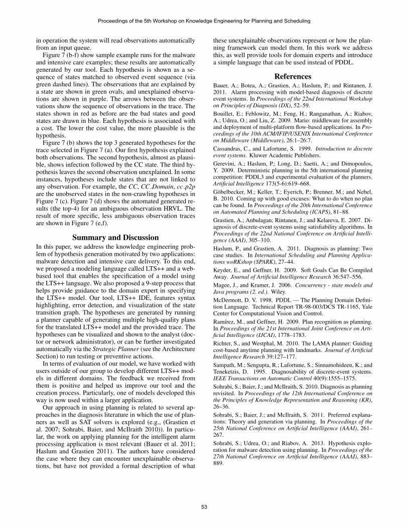
in operation the system will read observations automaticallyfrom an input queue.

Figure 7 (b-f) show sample example runs for the malwareand intensive care examples; these results are automaticallygenerated by our tool. Each hypothesis is shown as a se-quence of states matched to observed event sequence (viagreen dashed lines). The observations that are explained bya state are shown in green ovals, and unexplained observa-tions are shown in purple. The arrows between the obser-vations show the sequence of observations in the trace. Thestates shown in red as before are the bad states and goodstates are drawn in blue. Each hypothesis is associated witha cost. The lower the cost value, the more plausible is thehypothesis.

Figure 7 (b) shows the top 3 generated hypotheses for thetrace selected in Figure 7 (a). Our first hypothesis explainedboth observations. The second hypothesis, almost as plausi-ble, shows infection followed by the CC state. The third hy-pothesis leaves the second observation unexplained. In someinstances, hypotheses include states that are not linked toany observation. For example, the CC, CC Domain, cc p2pare the unobserved states in the non-crawling hypotheses inFigure 7 (c). Figure 7 (d) shows the automated generated re-sults (the top-4) for an ambiguous observation HRVL. Theresult of more specific, less ambiguous observation tracesare shown in Figure 7 (e,f).

Summary and DiscussionIn this paper, we address the knowledge engineering prob-lem of hypothesis generation motivated by two applications:malware detection and intensive care delivery. To this end,we proposed a modeling language called LTS++ and a web-based tool that enables the specification of a model usingthe LTS++ language. We also proposed a 9-step process thathelps provide guidance to the domain expert in specifyingthe LTS++ model. Our tool, LTS++ IDE, features syntaxhighlighting, error detection, and visualization of the statetransition graph. The hypotheses are generated by runninga planner capable of generating multiple high-quality plansfor the translated LTS++ model and the provided trace. Thehypotheses can be visualized and shown to the analyst (doc-tor or network administrator), or can be further investigatedautomatically via the Strategic Planner (see the ArchitectureSection) to run testing or preventive actions.

In terms of evaluation of our model, we have worked withusers outside of our group to develop different LTS++ mod-els in different domains. The feedback we received fromthem is positive and helped us improve our tool and thecreation process. Particularly, one of models developed thisway is now used within a larger application.

Our approach in using planning is related to several ap-proaches in the diagnosis literature in which the use of plan-ners as well as SAT solvers is explored (e.g., (Grastien etal. 2007; Sohrabi, Baier, and McIlraith 2010)). In particu-lar, the work on applying planning for the intelligent alarmprocessing application is most relevant (Bauer et al. 2011;Haslum and Grastien 2011). The authors have consideredthe case where they can encounter unexplainable observa-tions, but have not provided a formal description of what

these unexplainable observations represent or how the plan-ning framework can model them. In this work we addressthis, as well provide tools for domain experts and introducea simple language that can be used instead of PDDL.

ReferencesBauer, A.; Botea, A.; Grastien, A.; Haslum, P.; and Rintanen, J.2011. Alarm processing with model-based diagnosis of discreteevent systems. In Proceedings of the 22nd International Workshopon Principles of Diagnosis (DX), 52–59.Bouillet, E.; Feblowitz, M.; Feng, H.; Ranganathan, A.; Riabov,A.; Udrea, O.; and Liu, Z. 2009. Mario: middleware for assemblyand deployment of multi-platform flow-based applications. In Pro-ceedings of the 10th ACM/IFIP/USENIX International Conferenceon Middleware (Middleware), 26:1–26:7.Cassandras, C., and Lafortune, S. 1999. Introduction to discreteevent systems. Kluwer Academic Publishers.Gerevini, A.; Haslum, P.; Long, D.; Saetti, A.; and Dimopoulos,Y. 2009. Deterministic planning in the 5th international planningcompetition: PDDL3 and experimental evaluation of the planners.Artificial Intelligence 173(5-6):619–668.Gobelbecker, M.; Keller, T.; Eyerich, P.; Brenner, M.; and Nebel,B. 2010. Coming up with good excuses: What to do when no plancan be found. In Proceedings of the 20th International Conferenceon Automated Planning and Scheduling (ICAPS), 81–88.Grastien, A.; Anbulagan; Rintanen, J.; and Kelareva, E. 2007. Di-agnosis of discrete-event systems using satisfiability algorithms. InProceedings of the 22nd National Conference on Artificial Intelli-gence (AAAI), 305–310.Haslum, P., and Grastien, A. 2011. Diagnosis as planning: Twocase studies. In International Scheduling and Planning Applica-tions woRKshop (SPARK), 27–44.Keyder, E., and Geffner, H. 2009. Soft Goals Can Be CompiledAway. Journal of Artificial Intelligence Research 36:547–556.Magee, J., and Kramer, J. 2006. Concurrency - state models andJava programs (2. ed.). Wiley.McDermott, D. V. 1998. PDDL — The Planning Domain Defini-tion Language. Technical Report TR-98-003/DCS TR-1165, YaleCenter for Computational Vision and Control.Ramırez, M., and Geffner, H. 2009. Plan recognition as planning.In Proceedings of the 21st International Joint Conference on Arti-ficial Intelligence (IJCAI), 1778–1783.Richter, S., and Westphal, M. 2010. The LAMA planner: Guidingcost-based anytime planning with landmarks. Journal of ArtificialIntelligence Research 39:127–177.Sampath, M.; Sengupta, R.; Lafortune, S.; Sinnamohideen, K.; andTeneketzis, D. 1995. Diagnosability of discrete-event systems.IEEE Transactions on Automatic Control 40(9):1555–1575.Sohrabi, S.; Baier, J.; and McIlraith, S. 2010. Diagnosis as planningrevisited. In Proceedings of the 12th International Conference onthe Principles of Knowledge Representation and Reasoning (KR),26–36.Sohrabi, S.; Baier, J.; and McIlraith, S. 2011. Preferred explana-tions: Theory and generation via planning. In Proceedings of the25th National Conference on Artificial Intelligence (AAAI), 261–267.Sohrabi, S.; Udrea, O.; and Riabov, A. 2013. Hypothesis explo-ration for malware detection using planning. In Proceedings of the27th National Conference on Artificial Intelligence (AAAI), 883–889.


53

Creating Planning Domain Models in KEWI

Gerhard WicklerArtificial Intelligence Applications Institute

School of InformaticsUniversity of Edinburgh

[email protected]

Lukas Chrpa and Thomas Leo McCluskeyPARK Research Group

School of Computing and EngineeringUniversity of Huddersfield

{l.chrpa, t.l.mccluskey}@hud.ac.uk

Abstract

This paper reports on progress towards a tool for therepresentation of shared, procedural and declarativeknowledge whose aim is to be used for various func-tions to do with the automation of a complex processcontrol application - primarily to guide the responsephase during an emergency situation, but also for sup-porting normal automated operation.The tool is a Knowledge Engineering Web Interfacecalled KEWI. The focus of the paper is on the concep-tual model used to represent the declarative and proce-dural knowledge. The model consists of three layers: anontology, a model of basic actions, and more complexmethods. It is this structured conceptual model that fa-cilitates knowledge engineering. We are aiming to eval-uate the use of a central knowledge model for a range ofplanning-related functions, where the parts of the modelare automatically assembled e.g. into PDDL for opera-tional use.

IntroductionDomain-independent planning has grown significantly in re-cent years mainly thanks to the International Planning Com-petition (IPC). Besides many advanced planning engines,PDDL, a de-facto standard language family for describingplanning domain and problem models, has been developed.However, encoding domain and problem models in PDDLrequires a lot of specific expertise and thus it is very chal-lenging for a non-expert to use planning engines in applica-tions.

This paper concerns the use of AI planning technology inan organisation where (i) non-planning experts are requiredto encode knowledge (ii) the knowledge base is to be usedfor more than one planning and scheduling task (iii) it ismaintained by several personnel over a long period of time,and (iv) it may have a range of potentially unanticipated usesin the future. The first concern has been a major obstacleto using AI-based, formal representations, in that the exper-tise required to produce such representations has normallybeen acquired and encoded by planning experts (e.g. as inNASA’s applications (Ai-Chang et al. 2004)). The other con-cerns are often not covered in the planning literature: in realapplications the knowledge encoding is a valuable, generalasset, and one that requires a much richer conceptual rep-

resentation than, for example is accorded by planner-inputlanguages such as PDDL.

We present here a Knowledge Engineering method usinga Web Interface aimed at AI Planning, called KEWI. Theprimary idea behind KEWI then is to ease this formaliza-tion of procedural knowledge, allowing domain experts toencode their knowledge themselves, rather than knowledgeengineers having to elicit the knowledge before they formal-ize it into a representation. A number of frameworks ex-ist that support the formalization of planning knowledge inshared web-based systems. Usually, such frameworks buildon existing Web 2.0 technologies such as a wiki. A wiki thatsupports procedural knowledge is available at wikihow.com,but the knowledge remains essentially informal. A systemthat uses a similar approach, namely, representing procedu-ral knowledge in a wiki is CoScripter (Leshed et al. 2008).However, their representation is not based on AI planningand thus does not support the automated composition of pro-cedures. More recently, an AI-based representation has beenused in OpenVCE (Wickler, Tate, and Hansberger 2013).

As far as we are aware, very few collaborative, domain-expert-usable, knowledge acquisition interfaces are avail-able that are aimed at supporting the harvesting of planningknowledge within a rich language for use in a number ofplanning-related applications. After initial acquisition, thevalidation, verification, maintenance and evolution of suchsuch knowledge is of prime importance, as the knowledgebase is a valuable asset to an organisation.

Related WorkThere have been several attempts to create general, user-friendly development environments for planning domainmodels, but they tend to be limited in the expressivenessof their underlying formalism. The Graphical Interface forPlanning with Objects (GIPO) (Simpson, Kitchin, and Mc-Cluskey 2007) is based on object-centred languages OCLand OCLh. These formal languages exploit the idea that aset of possible states of objects are defined first, before ac-tion (operator) definition (McCluskey and Kitchin 1998).This gives the concept of a world state consisting of a setof states of objects, satisfying given constraints. GIPO usesa number of consistency checks such as if the object’s classhierarchy is consistent, object state descriptions satisfy in-variants, predicate structures and action schema are mutu-


54

ally consistent and task specifications are consistent with thedomain model. Such consistency checking guarantees thatsome types of errors can be prevented, in contrast to ad-hocmethods such as hand crafting.

itSIMPLE (Vaquero et al. 2012) provides a graphical en-vironment that enables knowledge engineers to model plan-ning domain models by using the Unified Modelling Lan-guage (UML). Object classes, predicates, action schema aremodelled by UML diagrams allowing users to ‘visualize’domain models which makes the modelling process easier.itSimple incorporates a model checking tool based on PetriNets that are used to check invariants or analyze dynamicaspects of the domain models such as deadlocks.

The Extensible Universal Remote Operations PlanningArchitecture (EUROPA) (Barreiro et al. 2012), is an inte-grated platform for AI planning and scheduling, constraintprogramming and optimisation. This platform is designed tohandle complex real-world problems, and the platform hasbeen used in some of NASA’s missions. EUROPA supportstwo representation languages, NDDL and ANML (Smith,Frank, and Cushing 2008), however, PDDL is not supported.

Besides these tools, it is also good to mentionVIZ (Vodrazka and Chrpa 2010), a simplistic tool inspiredby itSimple, and PDDL Studio (Plch et al. 2012), an editorwhich provides users a support by, for instance, identifyingsyntax errors or highlighting components of PDDL.

In the field of Knowledge Engineering, methodologieshave been developed which centre on the creation of a pre-cise, declarative and detailed model of the area of knowl-edge to be engineered, in contrast to earlier expert systemsapproaches which appeared to focus on the “transfer” ex-pertise at a more superficial level. This “expertise model”contains a mix of knowledge about the “problem solvingmethod” needed within the application and the declarativeknowledge about the application. Often a key rationale forknowledge engineering is to create declarative representa-tions of an area to act as a formalised part of some require-ments, making explicit what hitherto has been implicit incode, or explicit but in documents. Knowledge Engineer-ing modelling frameworks arose out of this, such as Com-monKads (Schreiber et al. 1999), which were based on adeep modelling of an area of expertise, and emphasisinga lifecycle of this model. The “knowledge model” withinCommonKADS, which contains a formal encoding of taskknowledge, such as problem statement(s), as well as domainknowledge, is similar to the kind of knowledge captured inKEWI. Unlike KEWI however, this model was expected tobe created by knowledge engineers rather than domain ex-perts and users.

Conceptual Model of KEWIKEWI is a tool for encoding domain knowledge mainlyby experts in the application area rather than AI planningexperts. The key idea behind KEWI is to provide a user-friendly environment as well as a language which is easier tofollow, especially for users who are not AI planning experts.A high-level architecture of KEWI is depicted in Figure 1.Encoded knowledge can be exported into the domain andproblem description in PDDL on which standard planning

Figure 1: An architecture of KEWI.

engines can be applied, and retrieved plans can be importedback to KEWI. Hence, the user does not have to understand,or even be aware, of any PDDL encodings.

A language in which domain knowledge is encoded inKEWI has three parts, which are explained in the followingsubsections. First, a domain ontology is defined. The do-main ontology consists of definition of classes of objects,hierarchies of classes and relations between objects. Sec-ond, action types, concretely action name, preconditions andeffects, are defined. Third, methods which introduce addi-tional ordering constraints between actions, are defined.

Ontology: Concepts, Relations and PropertiesOntological elements are usually divided into concepts andinstances. Typically, the concepts are defined in a planningdomain whereas the instances are defined in a planning prob-lem. Since our focus for KEWI is on planning domains weshall mostly deal with concepts here.

Concepts A concept is represented by a unique symbol inKEWI. The formal definition of a concept is given by itssuper-class symbol and by a set of role constraints that de-fine how instances of the concept may be related to otherconcepts. In KEWI, the definition of a concept also includesother, informal elements that are not used for formal rea-soning. However, the knowledge engineering value of suchinformal elements must not be underestimated, much likethe comments in programming often are vital for code to beunderstandable.

Definition 1 (KEWI Concept). A concept C in KEWI is apair 〈Csup, R〉, where:

• Csup is the direct super-concept of C and• R is a set of role constraints of the form 〈r, n, C ′〉 where r

is a symbolic role name,C ′ is a concept (denoting the rolefiller type), and n is a range [nmin, nmax] constrainingthe number of different instances to play that role.

We assume that there exists a unique root concept oftenreferred to as object or thing that acts as the implicit super-concept for those concepts that do not have an explicit super-concept defined in the same planing domain. Thus, a conceptC may be defined as 〈4, R〉, meaning its super concept isimplicit. This implicit super-concept has no role constraintsattached.

For example, in the Dock Worker Robot (DWR) domain,the concepts container and pallet could be definedwith the super-concept stackable, whereas the concept


55

crane could be defined as a root concept with no super-concept (implicitly:4). A role constraint can be used to de-fine that a crane can hold at most one container as follows:〈holds, [0, 1], container〉.

Since super-concepts are also concepts, we can write aconcept C as 〈〈〈4, Rn〉, . . . , R2〉, R1〉. Then we can re-fer to all the role constraints associated with C as R∗ =Rn ∪ . . . ∪ R2 ∪ R1, that is, the role constraints that ap-pear in the definition of C, the role constraints in its di-rect super-concept, the role constraints in its super-conceptssuper-concept, etc.

The reason for introducing this simple ontology of con-cepts is that we can now constrain the set of possible worldstates based on the role constraints. States are defined as setsof ground, first-order atoms over some function-free lan-guageL. This language shall contain symbols to denote eachinstance of a concept defined in the ontology (c1, . . . , cL)where the type function τ maps each instance ci to its typeC, a concept in the ontology. The relation symbols of L aredefined through the role constraints.

Definition 2 (Relations in L). Let 〈r, n, C ′〉 be a role con-straint of some concept C. Then the first-order language Lthat can be used to write ground atoms in a state contains abinary relation C.r ⊆ C × C ′.

In what follows we shall extend the language to includefurther relation symbols, but for now these relations definedby the ontology are all the relations that may occur in a state.The reason why the relation name is a combination of theconcept and the role is simply to disambiguate between rolesof the same name but defined in different concepts. Whereall role names are unique the concept may be omitted.

We can now define what it means for a state to be validwith respect to an ontology defined as a set of KEWI con-cepts. Essentially, for a state to be valid, every instance men-tioned in the state must respect all the role constraints associ-ated with the concepts to which the instance belongs. Sincerole constraints are constraints on the number of possiblerole fillers we need to be able to count these.

Definition 3 (Role Fillers). Let s be a state, that is, a setof ground atoms over objects c1, . . . , cL using the relationsin L. Let 〈r, n, C ′〉 be a role constraint of some concept C.Then we define valss(C.r, ci) = {cf |C.r(ci, cf ) ∈ s}, ci ∈C, cf ∈ C ′, that is, the set of all constants that play role rfor ci in s.

Definition 4 (Valid State). Let C be a KEWI concept. Thena state s is valid if, for any instance ci of C and anyrole constraint 〈r, n, C ′〉 of C or one of its (direct and in-direct) super-concepts, the number of ground atoms a =C.r(ci, ∗) must be in the range [nmin, nmax], i.e. nmin ≤|valss(C.r, ci)| ≤ nmax.

Thus, a concept definition defines a set of role constraintswhich can be interpreted as relations in a world state. Thenumeric range defines how many ground instances we mayfind in a valid state. This is the core of the ontological modelused in KEWI.

For example, let k1 be a crane and ca be acontainer. Then a state may contain a ground atom

crane.holds(k1,ca). If a state contains this atom, it maynot contain another one using the same relation and k1 asthe first argument.

Relations While the relations defined through the con-cepts in KEWI provide a strong ontological underpinningfor the representation, there are often situations where otherrelations are more natural, e.g. to relate more than two con-cepts to each other, or where a relation does not belong toa concept. In this case relations can be defined by declaringnumber and types (concepts) of the expected arguments.Definition 5 (Relations in L). A relation may be defined bya role constraint as described above, or it may be a relationsymbol followed by an appropriate number of constants. Thesignature of a relation R is defined as C1 × . . .×CR whereCi defines the type of the ith argument.

A valid state may contain any number of ground instancesof these relations. As long as the types of the constants inthe ground atoms agree with the signature of the relation,the state that contains this atom may be valid.

Properties In reality, we distinguish three different typesof role constraints: related classes for defining arbitrary re-lations between concepts, related parts which can be used todefine a “part-of” hierarchy between concepts, and proper-ties which relate instances to property values.

The first two are equivalent in the sense that they relateobjects to each other. However, properties usually relate val-ues to objects, e.g. an object may be of a given colour. Whileit often makes sense to distinguish all individual instances ofa concept, this is not true for properties. While the paint thatcovers one container may not be the same paint that coversanother, the colour may be the same. To allow for the repre-sentations of properties in KEWI, we allow for the definitionof properties with enumerated values.Definition 6 (Properties). A property P is defined as a setof constant values {p1, . . . , pP }.

It is easy to see that the above definitions relating torole constraints and other relations can be extended to allowproperties in place of concepts and property values in placeof instances. A minor caveat is that property values are usu-ally defined as part of a planning domain, whereas instancesare usually given in a planning problem.

Action TypesAction types in KEWI are specified using an operator namewith typed arguments, a set of preconditions, and a set ofeffects. This high-level conceptualization of action types isof course very common in AI planning formalisms. KEWI’srepresentation is closely linked with the ontology, however.This will enable a number of features that allow for a moreconcise representation, allowing to reduce the redundancycontained in many PDDL planning domains.

Object References In many action representations it isnecessary to introduce one variable for each object that issomehow involved in the execution of an action. This vari-able is declared as one of the typed arguments of the actiontype. The variable can then be used in the preconditions and


56

effects to consistently refer to the same objects and expressconditions on this object.

Sometimes, an action type may need to refer to specificconstants in its preconditions or effects. In this case, theunique symbol can be used to identify a specific instance.In the example above, k1 was used to refer to a crane andca to refer to a container. In most planning domains, opera-tor definitions do not refer to specific objects, but constantsmay be used as values of properties.

In addition to variables and constants, KEWI also allowsa limited set of function terms to be used to refer to objectsin an action type’s preconditions and effects. Not surpris-ingly, this is closely linked with the ontology, specificallywith the role constraints that specify a maximum of one intheir range.

Definition 7 (Function Terms). Let 〈r, n, C ′〉 be a role con-straint of some concept C where nmax = 1. Then we shallpermit the use of function terms of the form C.r(t) in pre-conditions and effects, where t can again be an arbitraryterm (constant, variable, or function term) of type C ′.

Let s be a valid state, that is, a set of ground atoms overobjects c1, . . . , cL using the relations inL. Then the constantrepresented by the function term C.r(ci) is:

• cj if valss(C.r, ci) = {cj}, or• nothing (⊥) if valss(C.r, ci) = ∅.

Note that the set valss(C.r, ci) can contain at most oneelement in any valid state. If it contains an element, this el-ement is the value of the function term. Otherwise a newsymbol that must not be one of the constants c1, . . . , cL willbe used to denote that the function term has no value. Thisnew constant nothing may also be used in preconditionsas described below.

The basic idea behind function terms is that they allow theknowledge representation to be more concise; it is no longernecessary to introduce a variable for each object. Also, thisstyle of representation may be more natural, e.g. to refer tothe container held by a crane as crane.holds(k1) mean-ing “whatever crane k1 holds”, where the role constrainttells us this must be a container. As a side effect, the gen-eration of a fully ground planning problem could be sim-pler,given the potentially reduced number of action parame-ters.

Interestingly, a step in this direction was already proposedin PDDL 1, in which some variables were declared as pa-rameters and others as “local” variables inside an operator.However, with no numeric constraints on role fillers or anyother type of relation, it is difficult to make use of such vari-ables in a consistent way. Similarly, state-variable represen-tations exploit the uniqueness of a value. However, this wasrestricted to the case where nmin and nmax both must beone.

Condition Types The atomic expressions that can be usedin preconditions and effects can be divided into two cat-egories. Firstly, there are the explicitly defined relations.These are identical in meaning and use to PDDL and thus,there is no need to discuss these further. Secondly, there arethe relations based on role constraints which have the same

form as such atoms in states, except that they need not beground.

Definition 8 (Satisfied Atoms). Let s be a valid state overobjects c1, . . . , cL. Then a ground atom a is satisfied in s(denoted s |= a) if and only if:

• a is of the form C.r(ci, cj) and a ∈ s, or• a is of the form R(ci1 , . . . , ciR) and a ∈ s, or• a is of the form C.r(ci,⊥) and valss(C.r, ci) = ∅.

The first two cases are in line with the standard semantics,whereas the the last case is new and lets us express that norole filler for a given instance exists in a given state. Notethat the semantics of atoms that use the symbol nothingin any other place than as a role filler are never satisfied inany state.

The above definition can now be used to define when anaction is applicable in a state.

Definition 9 (Action Applicability). Let s be a valid stateand act be an action, i.e. a ground instance of an action typewith atomic preconditions p1, . . . , pa. Then act is applicablein s if and only if every precondition is satisfied in s: ∀p ∈p1, . . . , pa : s |= p.

This concludes the semantics of atoms used in precondi-tions. Atoms used in effects describe how the state of theworld changes when an action is applied. This is usually de-scribed by the state transition function γ : S×A→ S, i.e. itmaps a state and an applicable action to a new state. Essen-tially, γ modifies the given state by deleting some atoms andadding some others. Which atoms are deleted and which areadded depends on the effects of the action. If the action isnot applicable the function is undefined.

Definition 10 (Effect Atoms). Let s be a valid state and actbe an action that is applicable in s. Then the successor stateγ(s, a) is computed by:

1. deleting all the atoms that are declared as negative effectsof the action,

2. for every positive effect C.r(ci, cj) for role constraint〈r, n, C ′〉 with n = [nmin, 1], if C.r(ci, ck) ∈ s deletethis atom, and

3. add all the atoms that are declared as positive effects ofthe action.

Following this definition allows for a declaration of ac-tions using arbitrary relations and state-variables that mayhave at most one value. The ontology, more specifically thenumeric role constraints can be used to distinguish the twocases.

The symbol nothing is not allowed in effects in KEWI.Of course, it would be easy to define the semantics of sucha construct as one that retracts all such atoms from the state.However, we have chosen not to go this way in KEWI fortwo reasons. Firstly, this construct would severely restrictthe number of planners that can handle this mass retraction,although it may be possible to express this as a universallyquantified effect. Secondly, it is not clear what an exampleof such an action would be in practise.


57

MethodsThe definition of methods in KEWI is not yet finished. Asthe framework is at least partially application-driven, wemay need to further refine the conceptual framework out-lined (but not fully defined) below.

The approach adopted in KEWI follows standard HTNplanning concepts: a method describes how a larger task canbe broken down in into smaller tasks which, together, ac-complish the larger task.

A method is defined by a method name with some pa-rameters. The name usually suggests how something is tobe done and the parameters have the same function as inaction types; they are the objects that are used or manipu-lated during the instantiation of a method. Next, a methodmust declare the task that is accomplished by the method.This is defined by a task name usually describing what isto be done, and again some parameters. For primitive tasks,the task name will be equal to the name of an action type,in which case no further refinement is required. For non-primitive tasks, a method also includes a set of subtasks.In KEWI, the ordering constraints between subtasks are de-clared with the subtask, rather than as a separate componentof the method. This is simply to aid readablility and does notchange the expressiveness.

In addition, to these standard components, KEWI allowsthe specification of high-level effects and subgoal-subtasks.The aim here is to allow for a representation that supportsflat, PDDL-like planning domains as well as hierarchicalplanning domains.

When a method declares that it achieves a high-level ef-fect, then every decomposition of this method must resultin an action sequence which will achieve the high-level ef-fect after the last action of the sequence has been completed.This could allow a planner to use a method as if it was an ac-tion in a backward search. An alternative view is that such amethod functions as a macro action type in the domain.

A method may also include subtasks that are effectivelysubgoals. For example, the subtask “achieve C.r(ci, cj)”may be used to state that at the corresponding point in thesubtask the condition C.r(ci, cj) must hold in the state. Theidea being that a planner may revert to flat planning (suchas state-space search) to find actions to be inserted into theplan at this point, until the subgoal is achieved.

This mixed approach is not new and has been used inpractical planners like O-Plan (Currie and Tate 1991). How-ever, the semantics has not been formally defined for thisapproach, something we shall attempt in future work.

Export to PDDLGiven that most modern planners accept planning domainsand problems in PDDL syntax as their input, one of thegoals for KEWI was to provide a mechanism that exportsthe knowledge in KEWI to PDDL. Of course, this will notinclude the HTN methods as PDDL does not support hierar-chical planning formalisms.

Function Terms The first construct that must be removedfrom KEWI’s representation are the function terms that may

be used to refer to objects. In PDDL’s preconditions and ef-fects only variables (or symbols) may be used to refer toobjects. The following function can be used to eliminate afunction term of the form C.r(t) that occurs in an actiontype O’s preconditions or effects.

function eliminate-fterms(C.r(t), O)if is-fterm(t) then

eliminate-fterms(t, O)v ← get-variable(C.r(t), O)replace every C.r(t) in O by v

The function first tests whether the argument to the givenfunction term is itself a function term. If this the case, it hasto be eliminated first. This guarantees that, for the remainderof the function t is either a variable or a symbol. We then usethe function “get-variable” to identify a suitable variable thatcan replace the function term. Technically, this function mayreturn a symbol, but the treatment is identical, which is whywe shall not distinguish these cases here. The identificationof a suitable variable then works as follows.function get-variable(C.r(v), O)

for every positive precondition p of O doif p = C.r(v, v′) then

if is-fterm(v′) theneliminate-fterms(v′, O)

return v′retrieve 〈r, n, C ′〉 from Cadd new parameter v′ of type C ′ to Oadd new precondition C.r(v, v′) to Oreturn v′

This function first searches for an existing, positive pre-condition that identifies a value for the function. Since func-tion terms may only be used for constraints that have at mostone value, there can only be at most one such precondition.If such a precondition exists, its role filler (v′, a variable ora symbol) may be used as the result. If no such preconditioncan be found, the function will create a new one and add itto the operator. To this end, a new parameter must be addedto the action type, and to know the type of the variable weneed to retrieve the role filler type from the role constraint.In practise, we also use the type name to generate a suitablevariable name. Then a new precondition can be added thateffectively binds the function to the role filler. And finally,the new variable may be returned.

Handling nothing The next construct that needs to beeliminated from the KEWI representation is any precondi-tion that uses the role filler nothing. Note that this symboldoes not occur in states and thus cannot be bound in tradi-tional PDDL semantics. Simply adding this symbol to thestate is not an option since other preconditions that require aspecific value could then be unified with this state atom. Forexample, if we had an explicit atom that stated holds(k1,nothing) in our state, then the precondition holds(?k,?c) of the load action type would be unifiable with thisatom. An inequality precondition may solve this problem,


58

but only if the planner can correctly handle inequalities. Thealternative approach we have implemented in KEWI is de-scribed in the following algorithm.

function eliminate-nothing(O)for every precondition p = C.r(v,⊥) do

replace p with C.r. ⊥ (v)if O has an effect e = C.r(v, v′)

add another effect ¬C.r. ⊥ (v)

The basic idea behind this approach is to use a new pred-icate to keep track of state-variables that have no values ina state. This is the purpose of the new predicate “C.r. ⊥”,indicating the role r of concept C has no filler for the givenargument. This is a common approach in knowledge engi-neering for planning domains. For example, in the classicblocks world we find a “holds” relation for when a block isbeing held, and a predicate “hand-empty” for when no blockis held.

The algorithm above uses this technique to replace all pre-conditions that have nothing as a role filler with a differ-ent precondition that expresses the non-existence of the rolefiller. To maintain this condition, it will also be necessaryto modify the effects accordingly. This is done by addingthe negation of this new predicate to corresponding existingeffects.

Since this is pseudo code, the algorithm actually omits afew details, e.g. the declaration of the new predicate in thecorresponding section of the PDDL domain, and the fact thatthe planning problem also needs to be modified to accountfor the new predicate. Both is fairly straight forward to im-plement.

State-Variable Updates Finally, the cases in which thevalue of a state-variable is simply changed needs to be han-dled. The approach we have adopted here is identical to theapproach described in (Ghallab, Nau, and Traverso 2004).That is, when an effect assigns a new value to a state vari-able, e.g. C.r(v, vnew), we need to add a precondition toget the old value, e.g. C.r(v, vold), and then we can usethis value in a new negative effect to retract the old value:¬C.r(v, vold).

ExampleIn this section we shall look at a single operator taken fromthe DWR domain and compare its representation in PDDLas defined in (Ghallab, Nau, and Traverso 2004) with theequivalent operator in KEWI. Note that this comparisondoes not include the representation of the underlying ontol-ogy, which is rather trivial in the case of the PDDL versionof the domain. However, there is one fundamental differencein the two ontologies, namely, that the PDDL version usesjust one symbol pallet to denote all the pallets which areat the bottom of each pile. We consider this epistemologi-cally inadequate. To avoid this discussion, we shall look atthe move operator here, which does not interact with piles ofcontainers directly, and therefore this ontological differencedoes not show up. In the PDDL version, the operator looksas follows:

(:action move:parameters(?r - robot ?from ?to - location)

:precondition (and(adjacent ?from ?to)(at ?r ?from)(not (occupied ?to)))

:effect (and(at ?r ?to)(not (occupied ?from))(occupied ?to)(not (at ?r ?from))))

The move operator takes three arguments: the robot to bemoved and the two locations involved. There are three pre-conditions expressing that applicability of this operator de-pends on the two locations being adjacent, the robot initiallybeing at the location from which the action takes place, andthe destination location currently not being occupied. Notethat the latter is a negative precondition which cannot behandled by all planners. The effects come in pairs and aresomewhat redundant. The robot being at the destination ofcourse implies that this location is now occupied. Similarly,the location that has just been vacated by the robot is nownot occupied and the robot is not at that location.

The equivalent operator in KEWI exploits some of thefeatures described above. However, it is important to notethat the user interface does not provide a text editor that canbe used to modify a PDDL-like representation. Instead, itconsists of a web-form with fields for the various compo-nents that define an action type. For comparison, we haveprinted the internal KEWI representation in a Lisp-like syn-tax, which looks as follows:

(:action-type move(:arguments ( (?robot robot)(?from location) (?to location) ))

(:precondition (and(:relation adjacent( ?from ?to ))

(:constr location.occupied-by( ?from ?robot ))

(:constr location.occupied-by( ?to nothing ))))

(:effect (and(:constr location.occupied-by( ?to ?robot ))

(:constr :not location.occupied-by( ?from ?robot )))))

The KEWI version of this operator also requires three pa-rameters. This is because none of the parameters is uniquelyimplied by any of the others. However, this is the only actionin the DWR domain for which this is the case. All actionsinvolving a crane have the location of the crane as anotherparameter, which would not be required in the KEWI ver-sion. The number of preconditions is not reduced either inthis case. However, the KEWI version of the operator doesnot require a negative precondition since it exploits onto-logical knowledge about the occupancy of locations. Thus,this precondition can be reformulated using the nothing


59

symbol. The biggest difference between the two representa-tions is in the effects, where KEWI only requires one effectfor each of the pairs listed above. Again, this is due to theontology that can be exploited, specifically to the fact thatlocation can only be occupied by one robot at a time. Nothaving to represent such redundant effects reduces the riskof knowledge engineers forgetting to list such effects. Notethat the second effect is negative, but could perhaps be ex-pressed more elegantly by using the nothing symbol asin the preconditions. This is not permitted in the syntax atpresent.

EvaluationThis work is being carried out with an industrial partner withsignificant experience in control and automation as well assimulation, and we are using a real application of knowledgeacquisition and engineering in their area of expertise. Thedevelopment of KEWI is in fact work in progress, and itsevaluation is ongoing, and being done in several ways: (i) Anexpert engineer from the industrial partner is using KEWI,in parallel with the developers, to build up a knowledge baseof knowledge about artefacts, operations, procedures etc. intheir domain. (ii) We have created a hand-crafted PDDLdomain and problem descriptions of part of the partner’sdomain and for the same problem area we have generatedPDDL automatically from a tool inside KEWI. We are inthe process of comparing the two methods and the PDDLproduced. An interface to a simulation system is being de-veloped which will help in this aspect. (iii) We are workingwith another planning project in the same application, whichaims to produce natural language explanations and argumen-tation supporting plans. In the future we believe to combineKEWI with this work, in order that (consistent with involv-ing the user in model creation) the user will be able to bettervalidate the planning operation.

ConclusionsIn this paper we have introduced a knowledge engineeringtool for building planning domain models, and given a for-mal account of parts of its structure and tools. Its characteris-tics are that (i) it has a user-friendly interface which is simpleenough to support domain experts in encoding knowledge(ii) it is designed so that it can be used to acquire a rangeof knowledge, with links to operation via automated trans-lators that create PDDL domain models (iii) it is designedto enable a groups of users to capture, store and maintainknowledge over a period of time, to enable the possibility ofknowledge reuse.

Acknowledgements

The research was funded by the UK EPSRC Au-tonomous and Intelligent Systems Programme (grant no.EP/J011991/1). The University of Edinburgh and researchsponsors are authorized to reproduce and distribute reprintsand online copies for their purposes notwithstanding anycopyright annotation hereon.

ReferencesAi-Chang, M.; Bresina, J. L.; Charest, L.; Chase, A.; jungHsu, J. C.; Jonsson, A. K.; Kanefsky, B.; Morris, P. H.;Rajan, K.; Yglesias, J.; Chafin, B. G.; Dias, W. C.; andMaldague, P. F. 2004. Mapgen: Mixed-initiative planningand scheduling for the mars exploration rover mission. IEEEIntelligent Systems 19(1):8–12.Barreiro, J.; Boyce, M.; Do, M.; Frank, J.; Iatauro, M.;Kichkaylo, T.; Morris, P.; Ong, J.; Remolina, E.; and Smith,T. 2012. EUROPA: A platform for AI planning, scheduling,constraint programming, and optimization. In 4th Interna-tional Competition on Knowledge Engineering for Planningand Scheduling (ICKEPS).Currie, K., and Tate, A. 1991. O-Plan: The open planningarchiteture. Artificial Intelligence 52:49–86.Ghallab, M.; Nau, D.; and Traverso, P. 2004. AutomatedPlanning. Morgan Kaufmann.Leshed, G.; Haber, E. M.; Matthews, T.; and Lau, T. A.2008. Coscripter: automating & sharing how-to knowledgein the enterprise. In CHI, 1719–1728.McCluskey, T. L., and Kitchin, D. E. 1998. A tool-supportedapproach to engineering HTN planning models. In In Pro-ceedings of 10th IEEE International Conference on Toolswith Artificial Intelligence.Plch, T.; Chomut, M.; Brom, C.; and Bartak, R. 2012. In-spect, edit and debug PDDL documents: Simply and effi-ciently with PDDL studio. ICAPS12 System Demonstration4.Schreiber, G.; Akkermans, H.; Anjewierden, A.; de Hoog,R.; Shadbolt, N.; de Velde, W. V.; and Wielinga, B. J.1999. Knowledge Engineering and Management: The Com-monKADS Methodology. Cambridge, Mass.: MIT Press,2nd ed. edition.Simpson, R.; Kitchin, D. E.; and McCluskey, T. 2007. Plan-ning domain definition using gipo. Knowledge EngineeringReview 22(2):117–134.Smith, D. E.; Frank, J.; and Cushing, W. 2008. The anmllanguage. Proceedings of ICAPS-08.Vaquero, T. S.; Tonaco, R.; Costa, G.; Tonidandel, F.; Silva,J. R.; and Beck, J. C. 2012. itSIMPLE4.0: Enhancingthe modeling experience of planning problems. In Sys-tem Demonstration – Proceedings of the 22nd InternationalConference on Automated Planning & Scheduling (ICAPS-12).Vodrazka, J., and Chrpa, L. 2010. Visual design of planningdomains. In KEPS 2010: Workshop on Knowledge Engi-neering for Planning and Scheduling.Wickler, G.; Tate, A.; and Hansberger, J. 2013. Using sharedprocedural knowledge for virtual collaboration support inemergency response. IEEE Intelligent Systems 28(4):9–17.


60

icaps 2014icaps14.icaps-conference.org/proceedings/keps/keps_proceedings.pdfable set vs refers to...

Documents