Life Prediction of Wind Turbine Blades

Kyo Kook Jin, Mustafa Ghulam, Jin Ho Kim, Sung Kyu Ha Dept. of Mech. Eng., Hanyang University, Korea

sungkha@gmail.com

Beatriz Méndez López, Alvaro Gorostidi Eng. Dept., ACCIONA Windpower, Noain, Spain

SUMMARY

An advanced life prediction of a wind turbine blade subjected to creep and fatigue loading has been developed using micromechanics of failure (MMF) and accelerated test methods (ATM). The MMF, which was originally developed to predict the static strength of composites, was now extended to generate creep and fatigue master curves of a unidirectional ply from those of constituents. A life of a wind blade is then obtained using the master curves and load distribution calculated from finite element analysis of wind turbine blades.

Keywords: wind turbine blades, micromechanics of failure, fatigue, Life prediction

INTRODUCTION

In a design process of structures of composite materials, creep and fatigue tests are the most costly and time consuming processes. An experimental or analytical approach, which reduces the number of long-term tests without sacrificing the accuracy, has long been quested, especially in the certificate process of structures. This investigation is devoted to proposing a life prediction method of wind turbine blades with minimum number of tests by combining the MMF and the ATM (accelerated test methodology).

WIND TURBINE BLADES

Technical description of the HSCL Wind Turbine

An advanced life prediction method is presented for the wind turbine blade subjected to time varying loads. The wind turbine consist in the present work has 146 m diameter, three bladed, upwind rotor and stall-control with variable speed operation. The technical specifications of baseline wind turbine are shown in the Table 1.

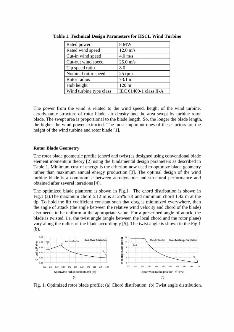
Table 1. Technical Design Parameters for HSCL Wind Turbine

Rated power 8 MW Rated wind speed 12.0 m/s Cut-in wind speed 4.0 m/s Cut-out wind speed 25.0 m/s Tip speed ratio 8.0 Nominal rotor speed 25 rpm Rotor radius 73.1 m Hub height 120 m Wind turbine type class IEC 61400-1 class II-A

The power from the wind is related to the wind speed, height of the wind turbine, aerodynamic structure of rotor blade, air density and the area swept by turbine rotor blade. The swept area is proportional to the blade length. So, the longer the blade length, the higher the wind power extracted. The most important ones of these factors are the height of the wind turbine and rotor blade [1].

Rotor Blade Geometry

The rotor blade geometric profile (chord and twist) is designed using conventional blade element momentum theory [2] using the fundamental design parameters as described in Table 1. Minimum cost of energy is the criterion now used to optimize blade geometry rather than maximum annual energy production [3]. The optimal design of the wind turbine blade is a compromise between aerodynamic and structural performance and obtained after several iterations [4].

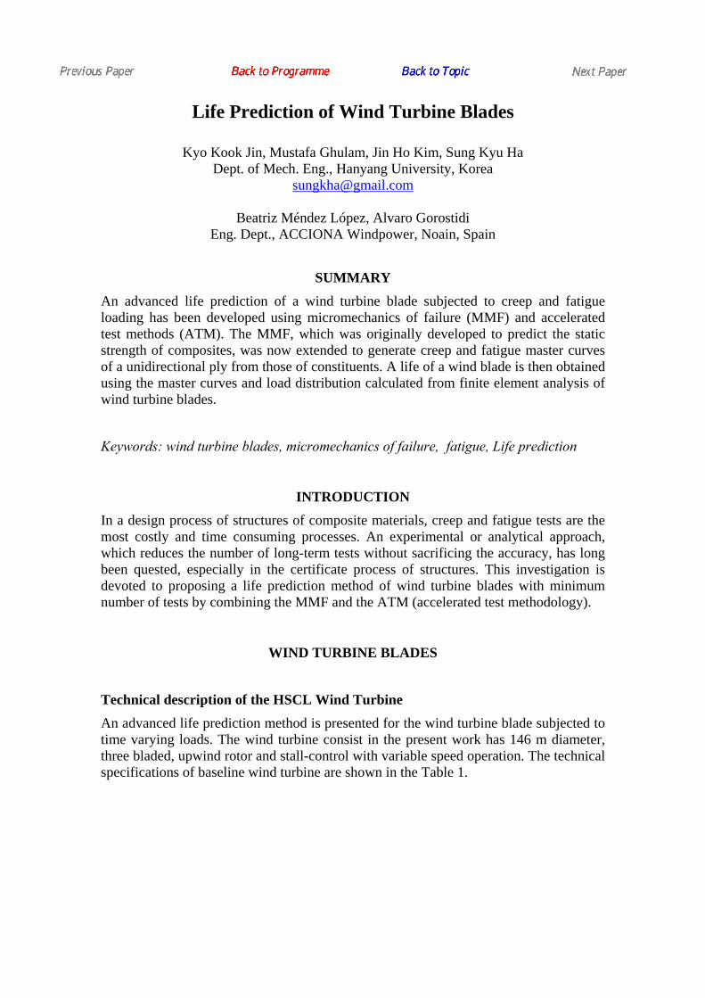
The optimized blade planform is shown in Fig.1. The chord distribution is shown in Fig.1 (a).The maximum chord 5.12 m is at 25% r/R and minimum chord 1.42 m at the tip. To hold the lift coefficient constant such that drag is minimized everywhere, then the angle of attack (the angle between the relative wind velocity and chord of the blade) also needs to be uniform at the appropriate value. For a prescribed angle of attack, the blade is twisted, i.e. the twist angle (angle between the local chord and the rotor plane) vary along the radius of the blade accordingly [5]. The twist angle is shown in the Fig.1 (b).

0.00

0.02

0.04

0.06

0.08

0.10

0.00 0.10 0.20 0.30 0.40 0.50 0.60 0.70 0.80 0.90 1.00

Blade Chord DistributionMax. chord location

Tip

Root

Ch

ord

, c/R

(%

)

Spanwise radial position, r/R (%)

(a)

0

3

6

9

12

15

0.00 0.10 0.20 0.30 0.40 0.50 0.60 0.70 0.80 0.90 1.00

Blade Twist Angle Distribution Max. chord location

Tip

Root

Spanwise radial position, r/R (%)

(b)

Twis

t an

gle

, (d

eg

ree

s)

Fig. 1. Optimized rotor blade profile; (a) Chord distribution, (b) Twist angle distribution.

Aerodynamic Design

The NREL S-series airfoils S816/S817/S818 are used for this current analysis [6]. The profile S818 is distributed in position between 25% r/R, and 75% r/R, S816 is distributed in position between 75% r/R and 90% r/R and S817 is distributed in position between 90% r/R and 100% r/R. The circular profile is selected for the inner part of the blade for strength purposes. The aerodynamic characteristics of the selected airfoils are in [6]. Fig. 2 depicts the overall blade topology.

(a) (b)

Fig. 2. Overall blade topology; (a) Airfoils, (b) Cross section at 30% r/R.

Baseline Structural Design of Rotor Blade

Several structural approaches for large blades are used now a day [7]. The blade has shell-spar structure[8] for current work. The typical structure of wind turbine blade at 30% r/R is shown in the Fig. 2 (b). The [02/+45] stacking sequence set as base laminate to both shell as well as shear webs and UD laminate to spar caps. The shell and shear webs is constructed with E-glass/LY556 Epoxy [9] and spar caps with IM6/Epoxy[10]. The laminate thickness at the shell, shear webs and spar caps were optimized iteratively, keeping strength ratio as design criterion, by using in-house developed spread-sheet based design tool 3D-Beam [11]. The maximum strength ratio calculated is 0.79.

Wind Turbine Blade Loads

There are three important sources of loading during operation of wind turbine as aerodynamic loads (mean wind speed & turbulent wind), gravity loads and centrifugal loads.

In order to simulate the aerodynamic loads as specified by IEC 61400-1[12], a three-dimensional wind field was simulated using Kaimal spectrum and coherence function described in the [13] along with wind shear.

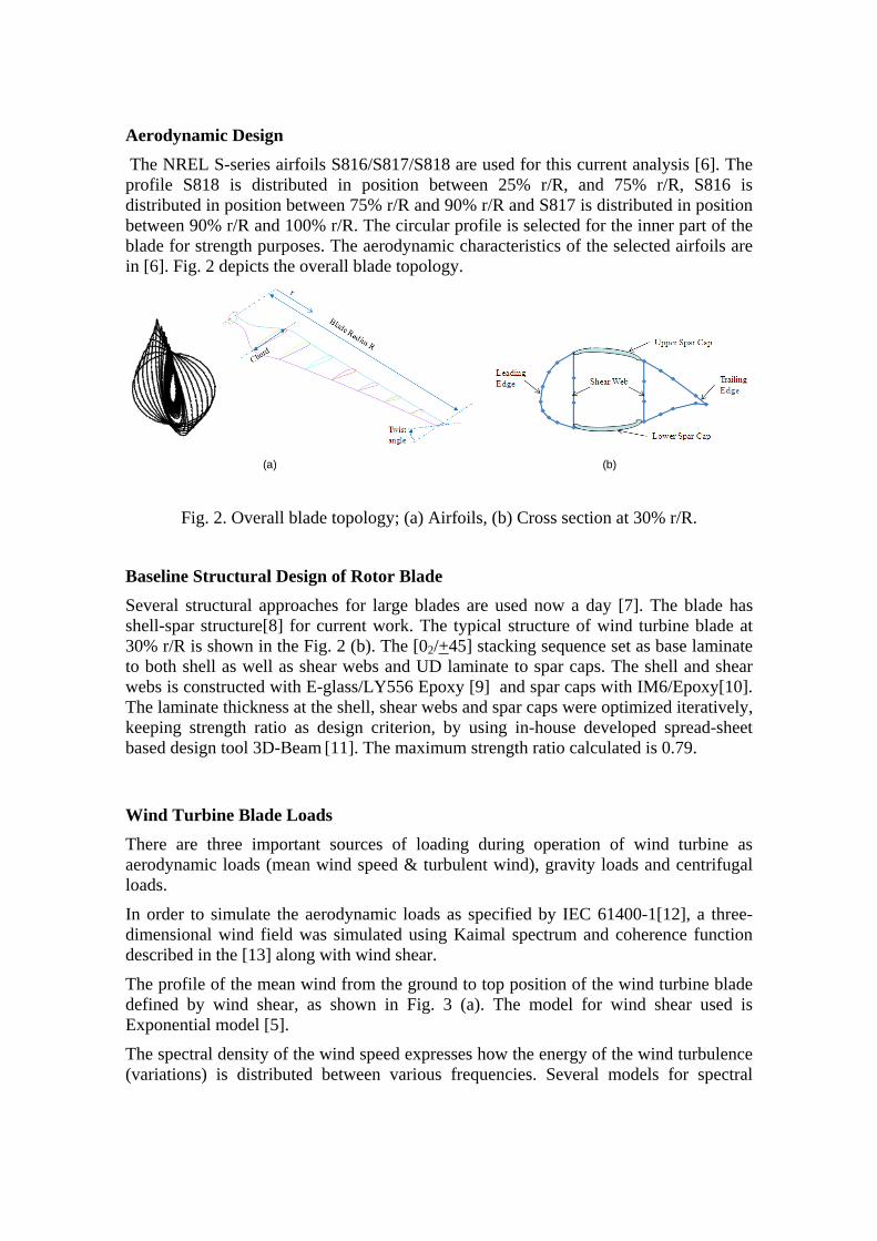
The profile of the mean wind from the ground to top position of the wind turbine blade defined by wind shear, as shown in Fig. 3 (a). The model for wind shear used is Exponential model [5].

The spectral density of the wind speed expresses how the energy of the wind turbulence (variations) is distributed between various frequencies. Several models for spectral

density exist [14]. A usually used model for spectral density is Kaimal [12], as shown in the Fig. 3 (b).

At any point in time there will be variability in the wind speed from one point to another. The closer together the two points are, the higher is the correlation between their respective wind speeds [14]. This can be described by coherence function (it is a frequency dependent measure of the amount of correlation between the wind speeds at two points in space), the coherence model used is given by Frost (1978) and also reported in [13].

(a)

0

50

100

150

200

250

300

350

400

450

0 5 10 15 20 25

Wind Shear ProfileExponential Model

He

igh

t, z

(m)

Velocity, U(z) (m/sec)

0.1

1

10

0.01 0.1 1 10

Kaimal Spectrum Model

Po

we

r S

pe

ctra

l De

nsi

ty(m

/se

c)^2

/Hz

Frequency, f (Hz)

(b)

Fig. 3. (a) Wind shear profile, (b) Kaimal power spectral density.

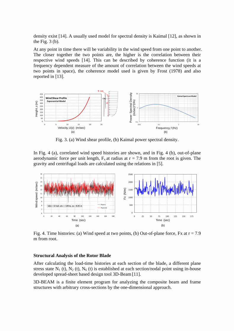
In Fig. 4 (a), correlated wind speed histories are shown, and in Fig. 4 (b), out-of-plane aerodynamic force per unit length, Fx at radius at r = 7.9 m from the root is given. The gravity and centrifugal loads are calculated using the relations in [5].

6

7

8

9

10

11

12

13

14

15

16

0 20 40 60 80 100 120 140 160 180

U(z) = 12 m/s at z = 120 m, zo = 0.01 mPoint 1

Point 10

(a)

Time (sec)

Win

d s

pe

ed

(m

/se

c)

(b)

0

500

1000

1500

2000

2500

0 25 50 75 100 125 150 175

Time (sec)

Fx

(N/m

)

Fig. 4. Time histories: (a) Wind speed at two points, (b) Out-of-plane force, Fx at r = 7.9 m from root.

Structural Analysis of the Rotor Blade

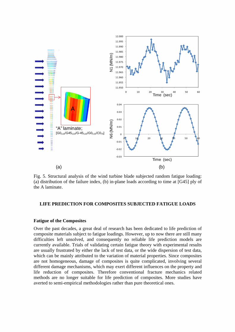
After calculating the load-time histories at each section of the blade, a different plane stress state N1 (t), N2 (t), N6 (t) is established at each section/nodal point using in-house developed spread-sheet based design tool 3D-Beam [11].

3D-BEAM is a finite element program for analyzing the composite beam and frame structures with arbitrary cross-sections by the one-dimensional approach.

‐0.03

‐0.02

‐0.01

0

0.01

0.02

0.03

0.04

0 10 20 30 40 50 60

11.950 

11.955 

11.960 

11.965 

11.970 

11.975 

11.980 

11.985 

11.990 

11.995 

12.000 

0 10 20 30 40 50 60

Time (sec)

Time (sec)

N6

(MN

/m)

(b)(a)

A

“A” laminate;[G0110/G45110/G-45110/G0110/C070]

N1

(MN

/m)

Fig. 5. Structural analysis of the wind turbine blade subjected random fatigue loading: (a) distribution of the failure index, (b) in-plane loads according to time at [G45] ply of the A laminate.

LIFE PREDICTION FOR COMPOSITES SUBJECTED FATIGUE LOADS

Fatigue of the Composites

Over the past decades, a great deal of research has been dedicated to life prediction of composite materials subject to fatigue loadings. However, up to now there are still many difficulties left unsolved, and consequently no reliable life prediction models are currently available. Trials of validating certain fatigue theory with experimental results are usually frustrated by either the lack of test data, or the wide dispersion of test data, which can be mainly attributed to the variation of material properties. Since composites are not homogeneous, damage of composites is quite complicated, involving several different damage mechanisms, which may exert different influences on the property and life reduction of composites. Therefore conventional fracture mechanics related methods are no longer suitable for life prediction of composites. More studies have averted to semi-empirical methodologies rather than pure theoretical ones.

Nevertheless, the recent development in both failure theories and testing methodologies casts light on the way towards resolving those previously mentioned obstacles. The micromechanics of failure (MMF), which is based on unit cell models of microstructure of composites, and independent constituent failure criteria, enables us to deal with failure in each constituent individually; the accelerated testing methodology (ATM), on the other hand, provides us with fatigue master curves of both fiber and matrix. In our view, the combination of MMF and ATM is a good candidate for fatigue life prediction of composite materials.

Life Prediction Method

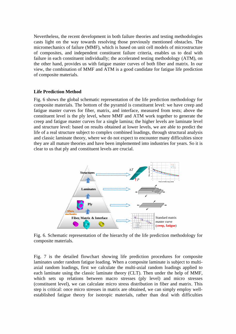
Fig. 6 shows the global schematic representation of the life prediction methodology for composite materials. The bottom of the pyramid is constituent level: we have creep and fatigue master curves for fiber, matrix, and interface, measured from tests; above the constituent level is the ply level, where MMF and ATM work together to generate the creep and fatigue master curves for a single lamina; the higher levels are laminate level and structure level: based on results obtained at lower levels, we are able to predict the life of a real structure subject to complex combined loadings, through structural analysis and classic laminate theory, where we do not expect to encounter many difficulties since they are all mature theories and have been implemented into industries for years. So it is clear to us that ply and constituent levels are crucial.

P

T

Fiber, Matrix & Interface

Ply

Laminates

Structures

0

20

40

60

80

100

120

0 1 2 3 4 5 6

T=25' C

T=70 'C

T=120 'C

Test Data

Max

. str

ess

[MP

a]

Time to Failure, log tf [min]

Standard matrix master curve(creep, fatigue)

Fig. 6. Schematic representation of the hierarchy of the life prediction methodology for composite materials.

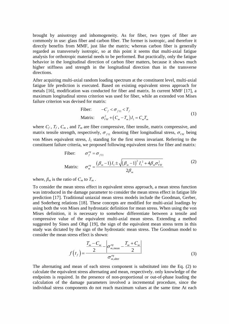
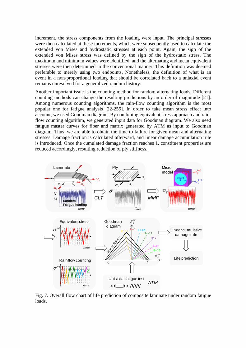
Fig. 7 is the detailed flowchart showing life prediction procedures for composite laminates under random fatigue loading. When a composite laminate is subject to multi-axial random loadings, first we calculate the multi-axial random loadings applied to each laminate using the classic laminate theory (CLT). Then under the help of MMF, which sets up relations between macro stresses (ply level) and micro stresses (constituent level), we can calculate micro stress distribution in fiber and matrix. This step is critical: once micro stresses in matrix are obtained, we can simply employ well-established fatigue theory for isotropic materials, rather than deal with difficulties

brought by anisotropy and inhomogeneity. As for fiber, two types of fiber are commonly in use: glass fiber and carbon fiber. The former is isotropic, and therefore it directly benefits from MMF, just like the matrix; whereas carbon fiber is generally regarded as transversely isotropic, so at this point it seems that multi-axial fatigue analysis for orthotropic material needs to be performed. But practically, only the fatigue behavior in the longitudinal direction of carbon fiber matters, because it shows much higher stiffness and strength in the longitudinal direction than in the transverse directions.

After acquiring multi-axial random loading spectrum at the constituent level, multi-axial fatigue life prediction is executed. Based on existing equivalent stress approach for metals [16], modification was conducted for fiber and matrix. In current MMF [17], a maximum longitudinal stress criterion was used for fiber, while an extended von Mises failure criterion was devised for matrix:

11

21

Fiber:

Matrix:

f f f

VM m m m m

C T

C T I C T

(1)

where Cf , Tf , Cm , and Tm are fiber compressive, fiber tensile, matrix compressive, and matrix tensile strength, respectively, 11f denoting fiber longitudinal stress, VM being

von Mises equivalent stress, I1 standing for the first stress invariant. Referring to the constituent failure criteria, we proposed following equivalent stress for fiber and matrix:

11

2 2 21 1

Fiber:

1 1 4Matrix:

2

eqf f

m m m VMeqm

m

I I

(2)

where, βm is the ratio of Cm to Tm .

To consider the mean stress effect in equivalent stress approach, a mean stress function was introduced in the damage parameter to consider the mean stress effect in fatigue life prediction [17]. Traditional uniaxial mean stress models include the Goodman, Gerber, and Soderberg relations [18]. These concepts are modified for multi-axial loadings by using both the von Mises and hydrostatic definition for mean stress. When using the von Mises definition, it is necessary to somehow differentiate between a tensile and compressive value of the equivalent multi-axial mean stress. Extending a method suggested by Sines and Ohgi [19], the sign of the equivalent mean stress term in this study was dictated by the sign of the hydrostatic mean stress. The Goodman model to consider the mean stress effect is shown:

,mean

,alter

2 2eqm m m mm

f eqm

T C T C

f t

(3)

The alternating and mean of each stress component is substituted into the Eq. (2) to calculate the equivalent stress alternating and mean, respectively. only knowledge of the endpoints is required. In the presence of non-proportional or out-of-phase loading the calculation of the damage parameters involved a incremental procedure, since the individual stress components do not reach maximum values at the same time At each

increment, the stress components from the loading were input. The principal stresses were then calculated at these increments, which were subsequently used to calculate the extended von Mises and hydrostatic stresses at each point. Again, the sign of the extended von Mises stress was defined by the sign of the hydrostatic stress. The maximum and minimum values were identified, and the alternating and mean equivalent stresses were then determined in the conventional manner. This definition was deemed preferable to merely using two endpoints. Nonetheless, the definition of what is an event in a non-proportional loading that should be correlated back to a uniaxial event remains unresolved for a generalized random history.

Another important issue is the counting method for random alternating loads. Different counting methods can change the resulting predictions by an order of magnitude [21]. Among numerous counting algorithms, the rain-flow counting algorithm is the most popular one for fatigue analysis [22-255]. In order to take mean stress effect into account, we used Goodman diagram. By combining equivalent stress approach and rain-flow counting algorithm, we generated input data for Goodman diagram. We also need fatigue master curves for fiber and matrix generated by ATM as input to Goodman diagram. Thus, we are able to obtain the time to failure for given mean and alternating stresses. Damage fraction is calculated afterward, and linear damage accumulation rule is introduced. Once the cumulated damage fraction reaches 1, constituent properties are reduced accordingly, resulting reduction of ply stiffness.

1N

2N6N

1M

2M

6M

NM

time

x s

y

time

( )mij

( )fij

(matrix)

( fiber )

ij

time

Laminate Ply Micro model

eq

time

Equivalent stress

CLT MMF

eq

time

Rainflow counting

R= -1

R= 0

R= -1.5 R= -0.5R= -0.3

R= 0.3

R= 0.5

eqa

eqm

C T

Goodman diagram

Uni-axial fatigue test

Linear cumulativedamage rule

Life prediction

RandomFatigue loading

ATM

Fig. 7. Overall flow chart of life prediction of composite laminate under random fatigue loads.

RESULTS

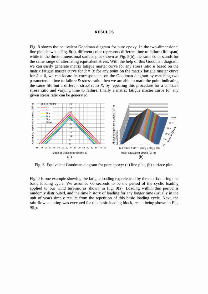
Fig. 8 shows the equivalent Goodman diagram for pure epoxy. In the two-dimensional line plot shown as Fig. 8(a), different color represents different time to failure (life span) while in the three-dimensional surface plot shown as Fig. 8(b), the same color stands for the same range of alternating equivalent stress. With the help of this Goodman diagram, we can easily generate matrix fatigue master curve for any stress ratio R based on the matrix fatigue master curve for R = 0: for any point on the matrix fatigue master curve for R = 0, we can locate its correspondent on the Goodman diagram by matching two parameters – time to failure & stress ratio; then we are able to mark the point indicating the same life but a different stress ratio R; by repeating this procedure for a constant stress ratio and varying time to failure, finally a matrix fatigue master curve for any given stress ratio can be generated.

0

5

10

15

20

25

30

35

40

45

50

80706050403020100‐10‐20‐30‐40‐50‐60‐70‐80

1 yr

5 yr

10 yr

20 yr

50 yr

100 yr

Mean equivalent stress (MPa)

Alte

rnat

ing

eq

uiva

lent

str

ess

(MP

a)

1 yr

5 yr

10 yr

20 yr

50 yr

100 yr

05101520253035404550

79

69

59

49

39

29

19 9 ‐1

‐11

‐21

‐31

‐41

‐51

‐61

‐71

‐81

‐91

Mean equivalent stress (MPa)

Alte

rativ

e eq

uiva

lent

str

ess

(MP

a)

Time to failure

(a) (b)

Fig. 8. Equivalent Goodman diagram for pure epoxy: (a) line plot, (b) surface plot.

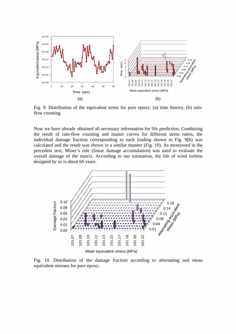
Fig. 9 is one example showing the fatigue loading experienced by the matrix during one basic loading cycle. We assumed 60 seconds to be the period of the cyclic loading applied to our wind turbine, as shown in Fig. 9(a). Loading within this period is randomly distributed, and the time history of loading for any longer time (usually in the unit of year) simply results from the repetition of this basic loading cycle. Next, the rain-flow counting was executed for this basic loading block, result being shown in Fig. 9(b).

101.00 

101.05 

101.10 

101.15 

101.20 

101.25 

101.30 

0 10 20 30 40 50 60

Time (sec)

Eq

uiv

ale

nt s

tre

ss (M

Pa

)

(b)(a)

Tim

e (

sec)

0.01 

0.04 

0.08 

0.11 

0.14 

0.18

0

1

2

3

4

5

101.07 

101.08 

101.09 

101.10 

101.11 

101.12 

101.13 

101.15 

101.16 

101.17 

101.18 

101.19 

101.20 

101.21 

Mean equivalent stress (MPa)

Fig. 9. Distribution of the equivalent stress for pure epoxy: (a) time history, (b) rain-flow counting.

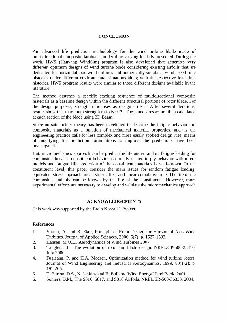
Now we have already obtained all necessary information for life prediction. Combining the result of rain-flow counting and master curves for different stress ratios, the individual damage fraction corresponding to each loading shown in Fig. 9(b) was calculated and the result was shown in a similar manner (Fig. 10). As mentioned in the precedent text, Miner’s rule (linear damage accumulation) was used to evaluate the overall damage of the matrix. According to our estimation, the life of wind turbine designed by us is about 66 years.

0.01 

0.04 

0.08 

0.11 

0.14 

0.18 

0.00

0.02

0.04

0.06

0.08

0.10

101.07 

101.09 

101.10 

101.12 

101.13 

101.15 

101.17 

101.18 

101.20 

101.22 

Dam

age

frac

tion

Mean equivalent stress (MPa)

Fig. 10. Distribution of the damage fraction according to alternating and mean equivalent stresses for pure epoxy.

CONCLUSION

An advanced life prediction methodology for the wind turbine blade made of multidirectional composite laminates under time varying loads is presented. During the work, HWS (Hanyang WindSim) program is also developed that generates very different optimum designs of wind turbine blade considering existing airfoils that are dedicated for horizontal axis wind turbines and numerically simulates wind speed time histories under different environmental situations along with the respective load time histories. HWS program results were similar to those different designs available in the literature.

The method assumes a specific stacking sequence of multidirectional composite materials as a baseline design within the different structural portions of rotor blade. For the design purposes, strength ratio uses as design criteria. After several iterations, results show that maximum strength ratio is 0.79. The plane stresses are then calculated at each section of the blade using 3D Beam.

Since no satisfactory theory has been developed to describe the fatigue behaviour of composite materials as a function of mechanical material properties, and as the engineering practice calls for less complex and more easily applied design rues, means of modifying life prediction formulations to improve the predictions have been investigated.

But, micromechanics approach can be predict the life under random fatigue loading for composites because constituent behavior is directly related to ply behavior with micro models and fatigue life prediction of the constituent materials is well-known. In the constituent level, this paper consider the main issues for random fatigue loading; equivalent stress approach, mean stress effect and linear cumulative rule. The life of the composites and ply can be known by the life of the constituents. However, more experimental efforts are necessary to develop and validate the micromechanics approach.

ACKNOWLEDGEMENTS

This work was supported by the Brain Korea 21 Project.

References

1. Vardar, A. and B. Eker, Principle of Rotor Design for Horizontal Axis Wind Turbines. Journal of Applied Sciences, 2006. 6(7): p. 1527-1533.

2. Hansen, M.O.L., Aerodynamics of Wind Turbines 2007. 3. Tangler, J.L., The evolution of rotor and blade design. NREL/CP-500-28410,

July 2000. 4. Fuglsang, P. and H.A. Madsen, Optimization method for wind turbine rotors.

Journal of Wind Engineering and Industrial Aerodynamics, 1999. 80(1-2): p. 191-206.

5. T. Burton, D.S., N. Jenkins and E. Bollany, Wind Energy Hand Book. 2001. 6. Somers, D.M., The S816, S817, and S818 Airfoils. NREL/SR-500-36333, 2004.

7. Tangler, J.L., The evolution of rotor and blade design. NREL/CP-500-28410, 2000.

8. Griffin, D.A., Blade system design studies Volume I: Composite technologies for large wind turbine blades. Sandia National Laboratories, Albuquerque, NM, 2002. SAND2002-1879.

9. Soden, P.D., M.J. Hinton, and A.S. Kaddour, Lamina properties, lay-up configurations and loading conditions for a range of fibre-reinforced composite laminates. Composites Science and Technology, 1998. 58(7): p. 1011-1022.

10. Tsai, S.W., Theory of composites design. 1992: Think Composites Dayton, Ohio. 11. Ha, S.K., User's Manual of 3D-Beam II, 3.19. 2009. 12. IEC, Wind turbine generator systems Part 1: Safety requirements. IEC 61400-1,

1999. 13. Veers, P.S. Three-dimensional wind simulation. 1988. 14. Riso/DNV, Guidelines for Design of Wind Turbines. 2002. 2nd Ed. 15. Matthew, M.D. and D.V. Kenneth, Numerical Implications of Solidity and Blade

Number on Rotor Performance of Horizontal-Axis Wind Turbines. Journal of Solar Energy Engineering, 2003. 125(4): p. 425-432.

16. G. Sines. Failure of Materials under combined repeated stresses superimposed with static stresses. Tech. Noth 3495, National Advisory Council for Aeronautics, Washington, D. C., 1955.

17. Ha SK, Jin KK, Huang YC. Micromechanics of failure (MMF) for continuous fiber reinforced composites. Journal of Composite Materials 2008; 42: 1873-1895.

18. Gang Tao, Zihui Xia (2008). Biaxial fatigue behavior of an epoxy polymer with mean stress effect, In press.

19. Shigley, J. E., and Mischke, C. R. (1989). Mechanical Engineering Design, McGraw-Hill, New York.

20. Sines, G., and Ohgi, G. (1981). Fatigue Criteria under Combined Stresses or Strains, ASME J. Eng. Mater. Technol., 103, pp. 82–90.

21. R. J. Bucci. Environment Enhanced Fatigue and Stress Corrosion Cracking of a Titanium Alloy Plus a Simple Model for the Assessment of Environmental Influence on Fatigue Behavior. Ph.D. Dissertation, Lehigh University, Bethlehem, Pa (1970).

22. M. Matsuishi and T. Endo, Fatigue of Metals Subjected to Varying Stress, JSME, Japan, 1968.

23. Downing, S. D., Socie, D. F. (1982). Simple rainflow counting algorithms. International Journal of Fatigue, Volume 4, Issue 1, January, 31-40.

24. ASTM E 1049-85. (Reapproved 2005). Standard practices for cycle counting in fatigue analysis. ASTM International.

25. Schluter, L. (1991). Programmer's Guide for LIFE2's Rainflow Counting Algorithm. Sandia Report SAND90-2260.