ices report 11-14 - university of texas at austin

A phase-field description of dynamic brittle fracture

M. J. Borden, C. V. Verhoosel, M. A. Scott, T. J. R. Hughes, and C. M. Landisby

ICES REPORT 11-14

May 2011

The Institute for Computational Engineering and SciencesThe University of Texas at AustinAustin, Texas 78712

Reference: M. J. Borden, C. V. Verhoosel, M. A. Scott, T. J. R. Hughes, and C. M. Landis, "A phase-field description ofdynamic brittle fracture", ICES REPORT 11-14, The Institute for Computational Engineering and Sciences, The University of Texas at Austin, May 2011.

A phase-field description of dynamic brittle fracture∗

Michael J. Borden1,† Clemens V. Verhoosel2 Michael A. Scott1

Thomas J. R. Hughes1 Chad M. Landis3

1Institute for Computational Engineering and SciencesThe University of Texas at Austin

1 University Station C0200, Austin, Texas 78712, USA2 Eindhoven University of Technology

Mechanical Engineering, Numerical Methods in EngineeringPO Box 513, WH 2.115, 5600 MB Eindhoven, The Netherlands

3 Aerospace Engineering & Engineering MechanicsThe University of Texas at Austin

1 University Station C0600, Austin, Texas 78712, USA

Abstract

In contrast to discrete descriptions of fracture, phase-field descriptions do not require numerical trackingof discontinuities in the displacement field. This greatly reduces implementation complexity. In this work,we extend a phase-field model for quasi-static brittle fracture to the dynamic case. We introduce a phase-field approximation to the Lagrangian for discrete fracture problems and derive the coupled system ofequations that govern the motion of the body and evolution of the phase-field. We study the behavior ofthe model in one dimension and show how it influences material properties. For the temporal discretizationof the equations of motion, we present both a monolithic and staggered time integration scheme. Westudy the behavior of the dynamic model by performing a number of two and three dimensional numericalexperiments. We also introduce a local adaptive refinement strategy and study its performance in the contextof locally refined T-splines. We show that the combination of the phase-field model and local adaptiverefinement provides an effective method for simulating fracture in three dimensions.

Keywords: Phase field, Fracture mechanics, Isogeometric analysis, Adaptive refinement, T-splines

1 IntroductionThe prevention of fracture-induced failure is a major constraint in engineering designs, and the numericalsimulation of fracture processes often plays a key role in design decisions. As a consequence, a wide varietyof fracture models have been proposed. A particularly successful model is provided by Griffith’s theory forbrittle fracture, which relates crack nucleation and propagation to a critical value of the energy release rate.A general concept in the Griffith’s-type brittle fracture models is that upon the violation of the critical energyrelease rate a fully opened crack is nucleated or propagated. As a consequence, the process zone, i.e., the∗Submitted to Computer Methods in Applied Mechanics and Engineering.†Corresponding author. Tel.: +1 512 475 6399; fax: +1 512 323 7508. E-mail address: [email protected]

1


zone in which the material transitions from the undamaged to the damaged state is lumped into a single pointat the crack tip.

Due to the complexity of fracture processes in engineering applications, numerical methods play a crucialrole in fracture analyses. In particular, finite element methods are used extensively in conjunction withGriffith’s-type linear elastic fracture mechanics models. Among the most commonly used finite elementmodels are the virtual crack closure technique (see Krueger (2004)), and, in more recent years, the extendedfinite element method introduced by Moes, Dolbow, and Belytschko (1999). All of these approaches representcracks as discrete discontinuities, either by inserting discontinuity lines by means of remeshing strategies, orby enriching the displacement field with discontinuities using the partition of unity method of Babuska andMelenk (1997). Tracing the evolution of complex fracture surfaces has, however, proven to be a tedious task,particularly in three dimensions.

Recently, alternative methods for the numerical simulation of brittle fracture have emerged. In theseapproaches, discontinuities are not introduced into the solid. Instead, the fracture surface is approximated bya phase-field, which smoothes the boundary of the crack over a small region. The major advantage of using aphase-field is that the evolution of fracture surfaces follows from the solution of a coupled system of partialdifferential equations. Implementation does not require the fracture surfaces to be tracked algorithmically.This is in contrast to the complexity of many discrete fracture models, and is anticipated to be particularlyadvantageous when multiple branching and merging cracks are considered in three dimensions.

A phase-field model for quasi-static brittle fracture emanated from the work of Bourdin and co-workerson the variational formulation for Griffith’s-type fracture models (see Bourdin, Francfort, and Marigo (2008)for a comprehensive overview). The variational formulation for quasi-static brittle fracture leads to an energyfunctional that closely resembles the potential presented by Mumford and Shah (1989), which is encounteredin image segmentation. A phase-field approximation of the Mumford-Shah potential, based on the theoryof Γ-convergence, was presented by Ambrosio and Tortorelli (1990). This approximation was adopted byBourdin, Francfort, and Marigo (2008) to facilitate the numerical solution of their variational formulation.Recently, this model has been applied in a dynamic setting by Bourdin, Larsen, and Richardson (2011);Larsen, Ortner, and Suli (2010); and Larsen (2010), but application to structures of engineering interest hasnot been considered.

An alternative quasi-static formulation of this phase-field approximation has been presented in the re-cent work of Miehe, Hofacker, and Welschinger (2010a) and Miehe, Welschinger, and Hofacker (2010b).In this formulation, the phase-field approximation follows from continuum mechanics and thermodynamicarguments. Besides the provision of an alternative derivation, Miehe, Hofacker, and Welschinger (2010a)also added various features to the model that are key to its application to engineering structures.

Independently from the phase-field formulation based on Griffith’s theory, dynamic phase-field fracturemodels have been developed based on Landau-Ginzburg type phase-field evolution equations, e.g., Karma,Kessler, and Levine (2001). However, we favor the phase-field formulation of the Bourdin-type since thephysical properties of Griffith’s theory are well understood and have proven useful in engineering applica-tions.

In this contribution we extend the quasi-static model presented by Miehe, Hofacker, and Welschinger(2010a) to the dynamic case. We begin by formulating the Lagrangian for the discrete fracture problemin terms of the displacements and the phase-field approximation of the crack path. Then, using the Euler-Lagrange equations of this approximation, we derive the strong form equations of motion. A detailed analysisof the analytical one-dimensional solution to the strong form equations is then presented. In this analysis weshow that although the length-scale parameter associated with the phase-field approximation is introducedas a numerical parameter it is, in fact, a material parameter that influences the critical stress at which cracknucleation occurs.

The numerical solution of the strong form of the equations of motion requires a spatial and temporal dis-cretization. We formulate the spatial discretization by means of the Galerkin method. In this work, we have

2


used NURBS and T-spline basis functions as the finite dimensional approximations to the function spacesof the weak form. However, we note that standard C0-continuous finite elements could also be used. Forthe temporal discretization, we present monolithic and staggered time integration schemes. The monolithicscheme requires solution of the coupled equations simultaneously. For the staggered scheme, the displace-ments (via the momentum equation) and phase-field (via the phase-field equation) are solved for separately.This provides flexibility in solution strategies by allowing the momentum equations to be solved either im-plicitly or explicitly.

To conclude this paper, we study the behavior of the model by performing a number of numerical bench-mark experiments for crack propagation and branching. These experiments show that the phase-field modelcan capture complex crack behavior in both two and three dimensions, without introducing any ad hoc crite-ria for crack nucleation and branching. In addition, we propose an adaptive refinement strategy that allowsfor the efficient simulation of complex crack patterns. We show that adaptive refinement maintains accuracywhile providing greater efficiency in terms of the number of degrees-of-freedom. Finally, we apply the adap-tive refinement strategy to a three-dimensional problem. This final problem illustrates the potential strengthof the phase-field model, which is the ability to efficiently model dynamic fracture in three-dimensions.

2 FormulationWe briefly introduce Griffith’s theory for dynamic brittle fracture in bodies with arbitrarily discrete cracks.We then present a phase-field formulation as a continuous approximation of the discrete fracture model. Weconclude this section with a study of analytical solutions of the phase-field in the one-dimensional quasi-staticcase, which reveals many interesting features of the model.

2.1 Griffith’s theory of brittle fractureWe consider an arbitrary body Ω ⊂ Rd (with d ∈ 1, 2, 3) with external boundary ∂Ω and internal dis-continuity boundary Γ (see Figure 1a). The displacement of a point x ∈ Ω at time t ∈ [0, T ] is denoted byu(x, t) ∈ Rd. Spatial components of vectors and tensors are indexed by i, j = 1, . . . , d. The displacementfield satisfies time-dependent Dirichlet boundary conditions, ui(x, t) = gi(x, t), on ∂Ωgi ⊆ ∂Ω, and time-dependent Neumann boundary conditions on ∂Ωhi ⊆ ∂Ω. We assume small deformations and deformationgradients, and define the infinitesimal strain tensor, ε(x, t) ∈ Rd×d, with components

εij = u(i,j) =1

2

(∂ui∂xj

+∂uj∂xi

)(1)

as an appropriate deformation measure. We assume isotropic linear elasticity, such that the elastic energydensity is given by

ψe(ε) =1

2λεiiεjj + µεijεij (2)

with λ and µ the Lame constants. Note that we use the Einstein summation convention on repeated indices.The evolving internal discontinuity boundary, Γ(t), represents a set of discrete cracks. In accordance with

Griffith’s theory of brittle fracture, the energy required to create a unit area of fracture surface is equal to thecritical fracture energy density Gc1. The total potential energy of the body, Ψpot, being the sum of the elasticenergy and the fracture energy, is then given by

Ψpot(u,Γ) =

∫Ω

ψe(∇su)dx+

∫Γ

Gcdx (3)

1This critical fracture energy density is commonly referred to as the critical energy release rate, or, in the context of cohesive zonemodels, the fracture toughness.

3


Ω

∂Ωgi

Γ

x1

x2

x3

∂Ωhi

Ω

∂Ωgi

c(x, t)

ǫ

x1

x2

x3

∂Ωhi

c = 0

c = 1

(a) (b)

Figure 1: (a) Schematic representation of a solid body Ω with internal discontinuity boundaries Γ. (b) Ap-proximation of the internal discontinuity boundaries by the phase-field c(x, t). The model parameter ε con-trols the width of the failure zone.

where we have defined the symmetric gradient operator, ∇s : u → ε, as a mapping from the displacementfield to the strain field. Since brittle fracture is assumed, the fracture energy contribution is merely the criticalfracture energy density integrated over the fracture surface. In the case of small deformations, irreversibilityof the fracture process dictates that Γ(t) ⊆ Γ(t + ∆t) for all ∆t > 0. Hence, translation of cracks throughthe domain is prohibited, but cracks can extend, branch, and merge.

The kinetic energy of the body Ω is given by

Ψkin(u) =1

2

∫Ω

ρuiuidx (4)

with u = ∂u∂t and ρ the mass density of the material. Combined with the potential energy (3) this renders the

Lagrangian for the discrete fracture problem as

L(u, u,Γ) = Ψkin(u)−Ψpot(u,Γ) =

∫Ω

[1

2ρuiui − ψe(∇su)

]dx−

∫Γ

Gcdx (5)

The Euler-Lagrange equations of this functional determine the motion of the body. From a numerical stand-point, tracking the evolving discontinuity boundary, Γ, often requires complex and costly computations. Thisis particularly so when interactions between multiple cracks (even in two dimensions), or complex shapedcracks in three dimensions are considered. Of particular interest in the case of dynamic fracture simulations,as considered in this work, is the ability to robustly model crack branching. In the remainder of this work wepursue a formulation which is capable of handling cracks of arbitrary topological complexity.

2.2 Phase-field approximationIn order to circumvent the problems associated with numerically tracking the propagating discontinuity rep-resenting a crack, we approximate the fracture surface, Γ, by a phase-field, c(x, t) ∈ [0, 1]. The value ofthis phase-field is equal to 1 away from the crack and is equal to 0 inside the crack (see Figure 1b). Weemploy the approximation as discussed in Miehe, Hofacker, and Welschinger (2010a), which is essentially

4


an extension of the phase-field approximation introduced by Bourdin, Francfort, and Marigo (2008)2. As inBourdin, Francfort, and Marigo (2008), we approximate the fracture energy by∫

Γ

Gcdx ≈∫Ω

Gc[

(c− 1)2

4ε+ ε

∂c

∂xi

∂c

∂xi

]dx (6)

where ε ∈ R+ is a model parameter that controls the width of the smooth approximation of the crack. Fromequation (6) it is clear that a crack is represented by regions where the phase-field, c(x, t), goes to zero. Aselaborated by e.g. Bourdin, Francfort, and Marigo (2008), in the limit of the length scale ε going to zero, thephase-field approximation converges to the discrete fracture surface.

To model the loss of material stiffness in the failure zone (i.e., the phase-field approximation of thefracture surface), the elastic energy is approximated by

ψe(ε, c) ≈ [(1− k)c2 + k]ψ+e (ε) + ψ−e (ε). (7)

As in Miehe, Hofacker, and Welschinger (2010a), we distinguish between the cases of compressive and ten-sile loading. By only applying the phase-field parameter to the tensile part of the elastic energy density,we prohibit crack propagation under compression. This model feature has been observed to be particularlyimportant in dynamic simulations, as stress waves reflecting from domain boundaries tend to create phys-ically unrealistic fracture patterns. The model parameter k 1 is introduced to prevent the positive partof the elastic energy density from disappearing when the phase-field is equal to zero, which has been ob-served to improve computational robustness in the quasi-static simulations presented by Miehe, Hofacker,and Welschinger (2010a).

Substitution of the phase-field approximations for the fracture energy (6) and the elastic energy density(7) into the Lagrange energy functional (5) yields

Lε(u, u, c) =

∫Ω

(1

2ρuiui − [(1− k)c2 + k]ψ+

e (∇su)− ψ−e (∇su)

)dx

−∫

Ω

Gc[

(c− 1)2

4ε+ ε

∂c

∂xi

∂c

∂xi

]dx.

(8)

Note that in order to conserve mass the kinetic energy term is unaffected by the phase-field approximation.The dependence of the Lagrange energy functional on the propagating discontinuity boundary is now capturedby the phase-field, c(x, t), which simplifies the numerical treatment of the model. In Miehe, Hofacker,and Welschinger (2010a) an additional viscosity contribution is introduced. For the dynamic simulationsperformed within this study no beneficial effects of this viscosity parameter were encountered, and hence thisterm is omitted for brevity.

Now that we have formulated the Lagrangian in terms of the independent fields u(x, t) and c(x, t), wecan use the Euler-Lagrange equations to arrive at the strong form equations of motion

∂σij∂xj

= ρui on Ω×]0, T [(4ε(1− k)ψ+

e

Gc+ 1

)c− 4ε2

∂2c

∂x2i

= 1 on Ω×]0, T [

(9)

2For the most part, we adopt the notation introduced by Bourdin, Francfort, and Marigo (2008), the exception being the use of k inplace of η for the model parameter that controls conditioning of the linear system. In Miehe, Hofacker, and Welschinger (2010a), use ismade of a damage field d(x, t) = 1− c(x, t), and a length scale l = 2ε to control the width of the failure zone.

5


where u = ∂2u∂t2 and the Cauchy stress tensor σ ∈ Rd×d is defined by

σij = [(1− k)c2 + k]∂ψ+

e

∂εij+∂ψ−e∂εij

. (10)

These equations of motion can be solved to find both the displacement field u(x, t) and phase-field c(x, t).The irreversibility condition Γ(t) ⊆ Γ(t + ∆t) is enforced in the strong-form equations by introducing astrain-history field,H, which satisfies the Kuhn-Tucker conditions for loading and unloading

ψ+e −H ≤ 0, H ≥ 0, H

(ψ+e −H

)= 0 (11)

(see Miehe, Hofacker, and Welschinger (2010a) for motivation on the introduction of H). After substitutingH for ψ+

e in (9)2 we get the modified strong form equations of motion

(S)

∂σij∂xj

= ρui on Ω×]0, T [(4ε(1− k)HGc

+ 1

)c− 4ε2

∂2c

∂x2i

= 1 on Ω×]0, T [.

(12)

The equations of motion are subject to the boundary conditions

(S: BC)

ui = gi on ∂Ωgi×]0, T [

σijnj = hi on ∂Ωhi×]0, T [

∂c

∂xini = 0 on ∂Ω×]0, T [

(13)

with gi(x, t) and hi(x, t) being prescribed on ∂Ωgi and ∂Ωhi, respectively, for all t ∈]0, T [, and with n(x)

being the outward-pointing normal vector of the boundary.In addition, the equations of motion (12) are supplemented with initial conditions

(S: IC)

u(x, 0) = u0(x) x ∈ Ω

u(x, 0) = v0(x) x ∈ Ω

c(x, 0) = c0(x) x ∈ Ω

(14)

for both the displacement field and the phase-field. The initial phase-field, c0(x), can be used to modelpre-existing cracks or geometrical features by setting it locally equal to zero (see Appendix A for details).

2.3 Analytical solutions of the one-dimensional quasi-static problemTo illustrate various properties of the phase-field formulation for brittle fracture, we study the analyticalsolution to the boundary value problem introduced in the previous section. We restrict ourselves to the one-dimensional domain Ω = R (d = 1) and ignore all temporal derivatives. In addition we assume the parameter

6


k to be equal to zero, and the strain field to be non-negative (i.e., ψ−e = 0 such that ψe = 12c

2Eε2). Underthese assumptions, the strong form equilibrium equations (12) reduce to

dσ

dx= 0 on R×]0, T [(

4εHGc

+ 1

)c− 4ε2

d2c

dx2= 1 on R×]0, T [

(15)

with σ = c2Eε. By virtue of (15)1, the stress σ is constant over the domain.

2.3.1 Homogeneous solution

We first study the homogeneous solution by ignoring all spatial derivatives of c. From the phase-field equationwe then obtain

chom =

(

2εEGc ε

2hom + 1

)−1

ψ+e = H (loading)(

4εGcH+ 1

)−1

ψ+e < H (unloading)

(16)

where chom and εhom are the homogeneous phase-field and strain, respectively. Substitution of this resultinto the constitutive equation yields the homogeneous stress as a function of the homogeneous strain

σhom =

(

2εEGc ε

2hom + 1

)−2

Eεhom ψ+e = H (loading)(

4εGcH+ 1

)−2

Eεhom ψ+e < H (unloading)

(17)

Figure 2(a) shows a characteristic plot of the homogeneous stress versus the homogeneous strain. Figure 2(b)shows the corresponding evolution of the homogeneous phase-field parameter. Note that the plotted resultshave been non-dimensionalized as outlined in Appendix B. It is observed that as the strain is increased,initially the stress also increases. This increase in stress is accompanied by a gradual decrease of the phase-field parameter. At some point, a critical stress level, σc, is reached after which both the stress and thephase-field decrease in value upon an increase in strain. In unloading the phase-field remains constant, whichresults in secant unloading behavior in the stress-strain curve.

As the critical stress indicates the state at which the material starts to soften, we refer to σc as the cracknucleation stress. The critical value for the stress, and corresponding value for the strain, are found as

σc =9

16

√EGc6ε

, εc =

√Gc

6εE(18)

From these expressions it is observed that the crack nucleation stress will increase as ε decreases. In thelimit as ε goes to zero, i.e., when the phase-field formulation coincides with the discrete fracture formulation,the crack nucleation stress becomes infinite. This observation is consistent with the properties of Griffith’stheory, which only allows for crack nucleation at stress singularities. It is interesting to note that the criticalvalue for the phase-field is independent of the model and material parameters

cc =

√σcEεc

=3

4. (19)

This implies that, no matter what parameters are used, a 25 percent reduction in the phase-field is establishedprior to crack nucleation at places where a crack emerges. At places where no crack is formed, the value

7


00

σ*c

σ*

ε*ε*c 0

0

1

3/4

c

ε*ε*c

(a) (b)

Figure 2: One-dimensional characteristic stress-strain (a) and phase-field-strain (b) curves for the homoge-neous solution. Note that the value of ε influences the maximum tensile stress, see (18).

of the phase-field scales with the ratio of the maximum stress in that point and the crack nucleation stress.Consequently, as the model parameter ε approaches zero, the phase-field will approach a value of one outsideof the fracture zone.

By virtue of the preceding analysis, we view ε as a material parameter since it influences the critical stressat which crack nucleation occures.

2.3.2 Non-homogenous solution

Additional interesting features of the model can be observed from the non-homogeneous solution of the one-dimensional static problem (15). If we ignore the irreversibility in the model, i.e. we takeH = 1

2Eε2, we can

combine the constitutive and phase-field equations to yield the non-linear ordinary differential equation(2εσ2

c4EGc+ 1

)c− 4ε2

d2c

dx2= 1. (20)

A solution for the phase-field, c(x), with a crack at x = 0 is found by supplementing this differential equationwith the boundary condition lim

x→±∞c(x) = chom(σ), which implies that the phase-field gradient vanishes far

away from the crack. It is important to note that the homogeneous solution to the phase-field is dependent onthe stress, σ, as elaborated in the previous section. In addition to the far-field boundary condition, we requirethe solution to be symmetric and differentiable at every point except for x = 0.

The first step in finding the non-homogeneous solution to the phase-field problem is to multiply equation(20) with dc

dx and make use of the fact that, by (15), σ is constant, to obtain

d

dx

[− εσ2

c2EGc+c2

2− 2ε2

(dc

dx

)2

− c

]= 0. (21)

Since we require the solution to be symmetric around x = 0, we integrate this expression from x to infinityfor positive values of x, and from minus infinity to x when x is negative. Since we have specified the crackto be centered at x = 0, we require the phase-field to have a minimum at x = 0. From these requirements,

8


we obtaindc

dx= sgn(x)

√1

2ε2

(− εσ2

c2EGc+c2

2− c− a

)(22)

where the coefficient a follows from the far-field boundary condition as

a = − εσ2

c2homEGc+c2hom

2− chom. (23)

By definition, substitution of the homogeneous solution chom(σ) into equation (22) yields a zero phase-field gradient. An analytical non-homogeous solution to equation (20) can be found for the case of a fullydeveloped crack, i.e. for σ = 0 (no stress carrying capability) and chom(0) = 1. In this case, equation (22)reduces to

dc

dx= sgn(x)

1− c2ε

. (24)

and, assuming c(0) = 0, we find

c = 1− exp

(−|x|

2ε

)(25)

as the solution that satisfies the specified boundary conditions. Note that this is the exact function used byMiehe et al. (2010a) to derive their phase field formulation.

The unique non-homogeneous solution can also be constructed for σ > 0. In this case, a second admiss-able phase-field value, smaller than the homogeneous solution, chom, for which the gradient is equal to zerocan be found. This phase-field value corresponds to the value of the phase-field at the center of the crack,and is denoted by ccrack. Since the phase-field increases monotonically from ccrack at the center of the crack(at x = 0) to chom far away from the crack (x = ±∞), we find the coordinates 0 < ±x < ∞ at which thephase-field is equal to ccrack < c(x) < chom by evaluation of

x = ±c(x)∫

ccrack

[1

2ε2

(− εσ2

c2EGc+c2

2− c− a

)]− 12

dc. (26)

In non-dimensional form with the non-dimensional constant Ch = 1, (26) becomes

x∗ = ±c(L0x

∗)∫ccrack

[1

2(ε∗)2

(−ε∗(σ∗)2

c2+c2

2− c− a∗

)]− 12

dc. (27)

Evaluating this integral numerically for σ = βσc with various values of β ∈]0, 1[ we get the solutions shownin Figure 3 (note that the presented results have again been non-dimensionalized and merely depend on theparameter β). It is interesting to note that, except for the limiting case of a fully developed crack, the solutionto the phase-field is smooth at the center of the crack.

3 Numerical formulationThe numerical solution of (12) requires a spatial and temporal discretization. In this section we formulatethe spatial discretization by means of the Galerkin method and we introduce two temporal discretizationschemes: a monolithic implicit scheme and a staggered scheme in which the momentum equation and phase-field equation are solve separately, and in which the momentum equation may be solved either by an explicitor implicit scheme.

9


1

0 x*

c

β00.250.50.75

Figure 3: One-dimensional solution of the phase field formulation for various values of the stress ratio β =σσc

= σ∗

σ∗c

. Note that, except for the limiting case β = 0, the phase-field is smooth at the center of the crack(x∗ = 0).

3.1 Continuous problem in the weak form

For the weak form of the problem we define the trial solution spaces St for the displacements and St for thephase-field as

St = u(t) ∈ (H1(Ω))d | ui(t) = gi on ∂Ωgi (28)

St = c(t) ∈ H1(Ω). (29)

Similarly, the weighting function spaces are defined as

V = w ∈ (H1(Ω))d | wi = 0 on ∂Ωgi (30)

V = q ∈ H1(Ω). (31)

Multiplying the equations in (12) by the appropriate weighting functions and applying integration by partsleads to the weak formulation:

(W)

Given g, h, u0, u0, and c0 find u(t) ∈ St and c(t) ∈ St, t ∈ [0, T ], such that for allw ∈ V and for all q ∈ V ,

(ρu,w)Ω + (σ,∇w)Ω = (h,w)∂Ωh((4ε(1− k)HGc

+ 1

)c, q

)Ω

+(4ε2∇c,∇q

)Ω

= (1, q)Ω

(ρu(0),w)Ω = (ρu0,w)Ω

(ρu(0),w)Ω = (ρu0,w)Ω

(c(0), q)Ω = (c0, q)Ω

(32)

where (•, •)Ω is the L2 inner product on Ω.

3.2 The semidiscrete Galerkin formFollowing the Galerkin method, we let Sht ⊂ St, Vh ⊂ V , Sht ⊂ St, and Vh ⊂ V be the usual finite-dimensional approximations to the function spaces of the weak form (see Hughes (2000) for details). The

10


semidiscrete Galerkin form of the problem is then given as

(G)

Given g, h, u0, u0, and c0 find uh(t) ∈ Sht and ch(t) ∈ Sht , t ∈ [0, T ], such that forall wh ∈ Vh and for all qh ∈ Vh,(

ρuh,wh)

Ω+(σ,∇wh

)Ω

=(h,wh

)∂Ωh((

4ε(1− k)HGc

+ 1

)ch, qh

)Ω

+(4ε2∇ch,∇qh

)Ω

=(1, qh

)Ω(

ρuh(0),wh)

Ω= (ρu0,w

h)Ω(ρuh(0),wh

)Ω

= (ρu0,wh)Ω(

ch(0), qh)

Ω= (c0, q

h)Ω

(33)

The explicit representations of uh,wh, ch, and qh in terms of the basis functions and nodal variables are

uhi =

nb∑A

NA(x)diA (34)

whi =

nb∑A

NA(x)ciA (35)

ch =

nb∑A

NA(x)φA (36)

qh =

nb∑A

NA(x)χA (37)

where nb is the dimension of the discrete space, the NA’s are the global basis functions, i is the spatialdegree-of-freedom number, and diA, ciA, φA, and χA are control variable degrees-of-freedom. Note that wehave assumed that both the finite dimensional trial solution and weighting function spaces are defined by thesame set of basis functions.

3.2.1 Isogeometric spatial discretization

In contrast to earlier work on phase-field models, we have chosen to use isogeometric spatial discretizations asintroduced by Hughes et al. (2005), which are based on NURBS and T-splines. T-splines are a generalizationof NURBS that allows greater flexibility in geometric design including local refinement. A class of analysis-suitable T-splines was identified in Li et al. (2010) and Scott et al. (2011). This class of T-splines preserves theimportant mathematical properties of NURBS while providing an efficient and highly localized refinementcapability. Analysis-suitable T-splines possess the following properties:

• Linear independence.

• The basis constitutes a partition of unity.

• Each basis function is non-negative.

• An affine transformation of an analysis-suitable T-spline is obtained by applying the transformation tothe control points. We refer to this as affine covariance. This implies that all patch tests (see Hughes(2000)) are satisfied a priori.

11


• They obey the convex hull property, see Piegl and Tiller (1997).

• Local refinement is possible.

For additional details on basic T-spline analysis technology see Scott et al. (2010).The spline-based analysis strategy of isogeometric analysis has shown some advantages when compared

to standard C0 finite elements. First, isogeometric analysis allows for the efficient and exact geometric rep-resentation of many objects of engineering interest. Also, when using T-spline-based isogeometric analysis,efficient and automatic local mesh refinement strategies exist that preserve the exact geometry. Secondly,the isogeometric basis is in general smooth. Although the phase-field model permits the use of traditionalC0 finite elements, the use of a smooth base is anticipated to have favorable effects. One is that stressesare represented more accurately than with traditional C0 finite elements, which has been observed to yieldefficient spatial discretizations for discrete (see Verhoosel et al. (2010)) and smeared (see Verhoosel et al.(2011)) fracture models. Another study by Benson et al. (2011) has shown that the accuracy of the spatialdiscretization of NURBS allows for more efficient time integration for explicit dynamics in the context oflarge deformation shells.

3.3 Time discretization and numerical implementation3.3.1 Monolithic generalized-α time discretization

The monolithic time integration scheme is based on the generalized-α method introduced by Chung andHulbert (1993). We define the residual vectors as

Ru = RuA,i, (38)

RuA,i = (h, NAei)∂Ωh−(ρuh, NAei

)Ω−(σjk, B

ijkA

)Ω

(39)

and

Rc = RcA, (40)

RcA = (1, NA)Ω −((

4ε(1− k)HGc

+ 1

)ch, NA

)Ω

−(

4ε2∂ch

∂xi,∂NA∂xi

)Ω

, (41)

where ei is the ith Euclidean basis vector and

BijkA =1

2

(∂NA∂xj

δik +∂NA∂xk

δij

)(42)

so that εjk =∑AB

ijkA dA,i. For time step n, let dn and φn be the vectors of control variable degrees-of-

freedom of the displacements and phase-field, respectively (see (34) and (36)). We then define vn = dn, andan = dn. The monolithic generalized-α time integration scheme is then stated as follows: given (dn, vn,an), find (dn+1, vn+1, an+1, dn+αf

, vn+αf, an+αm

, φn+1) such that

Ru(dn+αf,vn+αf

,an+αm,φn+1) = 0, (43)

Rc(dn+αf,φn+1) = 0, (44)dn+αf

= dn + αf (dn+1 − dn), (45)vn+αf

= vn + αf (vn+1 − vn), (46)an+αm

= an + αm(an+1 − an), (47)vn+1 = vn + ∆t((1− γ)an + γan+1), (48)

dn+1 = dn + ∆tvn +(∆t)2

2((1− 2β)an + 2βan+1), (49)

12


where ∆t = tn+1 − tn is the time step and the parameters αf , αm, β, and γ define the method. Theseparameters will be discussed below.

At each time step, the solution is obtained using a Newton-Raphson method to solve the nonlinear equa-tions above. Letting i be the Newton iteration, the residual vector and consistent tangent matrix for thelinearized system are defined by

∂Rui

∂an+1∆a+

∂Rui

∂φn+1

∆φ = −Rui , (50)

∂Rci

∂an+1∆a+

∂Rci

∂φn+1

∆φ = −Rci , (51)

where

Rui = Ru(din+αf

,vin+αf,ain+αm

,φn+1), (52)

and

Rci = Rc(dn+αf

,φn+1). (53)

For each iteration, the linearized system defined by (50) and (51) is solved and iteration continues untilconvergence of the residual vectors occurs. For the examples discussed below, we have defined convergenceas

max‖Ru

i ‖‖Ru

0‖,‖Rc

i‖‖Rc

0‖

≤ tol (54)

where ‖ · ‖ denotes the Euclidean norm. For the simulations considered in this work, tol = 10−4 has beenobserved to be an appropriate choice.

Parameter selection In Chung and Hulbert (1993) it was shown that αf and αm can be parametrizedby the spectral radius, ρ∞, of the amplification matrix at ∆t = ∞ such that second-order accuracy andunconditional stability are achieved for a second-order linear problem if

αf =1

ρ∞ + 1, (55)

αm =2− ρ∞ρ∞ + 1

, (56)

β =1

4(1 + αm − αf )2, (57)

γ =1

2+ αm − αf . (58)

3.3.2 Staggered time discretization

For the staggered time integration scheme, the momentum and phase-field equations are solved indepen-dently. At a given time step, the momentum equation is solved first to get the displacements. Using theupdated displacements, the phase-field equation is solved. In addition to reducing the problem to solving twolinear systems, this scheme also allows greater flexibility in how the momentum equation is solved, i.e., wecan use either implicit or explicit schemes. This scheme can also be generalize to a predictor/multicorrectorformat where additional Newton-Raphson iterations can be performed within a time step. Below we present

13


a general predictor/multicorrector algorithm, but for the results presented later we use only one pass of thecorrector stage.

Defining the residual vectors for the momentum and phase-field equations by (39) and (41), and again let-ting d andφ be arrays of the control variable coefficients in (34) and (36), the staggered predictor/multicorrectortime integration scheme is stated as follows: given (dn, vn, an, φn), solve

Predictor stage

i = 0 (iteration counter) (59)vn+1 = vn + ∆t(1− γ)an (60)

dn+1 = dn + ∆tvn +(∆t)2

2(1− 2β)an (61)

a(i)n+1 = 0 (62)

v(i)n+1 = vn+1 (63)

d(i)n+1 = dn+1 (64)

φ(i)n+1 = φn (65)

Multicorrector stage

a(i)n+αm

= an + αm(a(i)n+1 − an) (66)

v(i)n+αf

= vn + αf (v(i)n+1 − vn) (67)

d(i)n+αf

= dn + αf (d(i)n+1 − dn) (68)

M∗∆a = Ru(d(i)n+αf

v(i)n+αf

,a(i)n+αm

,φ(i)n+1) (69)

a(i+1)n+1 = a

(i)n+1 + ∆a (70)

v(i+1)n+1 = vn+1 + ∆tγa

(i+1)n+1 (71)

dn+1 = dn+1 + (∆t)2βa(i+1)n+1 (72)

Kcc∆φ = Fc (73)

φ(i+1)n+1 = ∆φ (74)

The phase-field arrays in (73) are defined as

Kcc = [KAB ], (75)

KAB =

((4ε(1− k)HGc

+ 1

)NB , NA

)Ω

+

(4ε2

∂NB∂xi

,∂NA∂xi

)Ω

, (76)

Fc = FA, (77)FA = (1, NA), (78)

and ∆t = tn+1 − tn is the time step and the parameters αm, αf , β, and γ, which define the method, areselected as described below.

If the linearized momentum equation (69) is being solved implicitly then

M∗ = − ∂Rui

∂an+1= αmM + αfβ(∆t)2K, (79)

14


where M is the consistent mass matrix and

K = [KuuAB,ij ], (80)

KuuAB,ij =

(∂σlk∂εmn

BjmnB , BilkA

)Ω

(81)

is the consistent damage-elastic tangent stiffness matrix. If we let M∗ = αmM where M is the lumpedmass matrix then the linearized momentum equation is solved explicitly. When computing with NURBS andT-splines, we compute M using the row-sum technique as described in Hughes (2000). Due to the fact thatNURBS and T-spline basis functions are point-wise positive, the row-sum lumped mass matrix is guaranteedto be positive. Furthermore, it is also mass conservative.

Parameter selection For the staggered solution strategy, the choice of αm, αf , and M∗ provides severaloptions for the type of algorithm that is used to solve the linear momentum problem. For the fully implicit case(M∗ = αmM + αfβ(∆t)2K) we use the generalized-α method described above. For the fully explicit case(M∗ = αmM) we use either the HHT-α of Hilber, Hughes, and Tayler (1977) or the explicit generalized-αmethod of Hulbert and Chung (1996). The HHT-α method, parameterized by α, provides a second-orderaccurate family of algorithms for linear second-order equations if α ∈ [− 1

3 , 0] and

αm = 1, (82)αf = 1 + α, (83)

β =(1− α)2

4, (84)

γ =1− 2α

2(85)

(see Miranda, Ferencz, and Hughes (1989)). The explicit generalized-α method, as shown by Hulbert andChung (1996), is a one-parameter family of explicit algorithms that provides optimal numerical dissipationand is second-order accurate for linear problems if αf = 0 and

αm =2− ρb1 + ρb

, (86)

β =5− 3ρb

(1 + ρb)2(2− ρb), (87)

γ = αm +1

2, (88)

where ρb is the spectral radius value at the bifurcation limit of the principal roots of the characteristic equation.

4 Numerical resultsIn this section we investigate the numerical performance of the phase-field fracture model. All geometrieshave been discretized spatially using either NURBS or T-spline basis functions (which we refer to as theglobal smooth basis). The numerical computation for all the models was performed using the Bezier ex-traction methods described by Borden et al. (2010) and Scott et al. (2010). Bezier extraction constructs theminimal set of Bezier elements defining a NURBS or T-spline. A Bezier element is a region of the physicaldomain in which the basis functions are C∞-continuous and over which integration is performed. In addition

15


to defining elements, Bezier extraction also builds an extraction operator for each Bezier element that mapsa Bernstein polynomial basis defined on the Bezier element to the global smooth basis. The transpose of theextraction operator maps the control points of the global smooth basis to the Bezier control points. The ideais illustrated in Figure 4 for a cubic B-spline curve. The B-spline curve with its control points, P = PI7I=1,and basis functions, N = NI7I=1, is shown on the left with the elements, Ωe, defined on the parametric do-main. On the right we illustrate the action of the extraction operator, C2 ∈ R4×4, for Ω2. The transpose of theextraction operator, CT

2 , defines the Bezier control points, Q2 = Q2,I4I=1, for the Bezier element in termsof the global control points, as shown in Figure 4. The Bernstein polynomial basis functions, B = BI4I=1,are shown below the Bezier element. The extraction operator is used to extract the smooth B-spline basisfunctions N2 = NI5I=2 from the Bernstein basis, i.e., the B-spline basis functions can be written as linearcombinations of the Bernstein basis functions. Bezier extraction provides a completely local representationof the global smooth basis. It provides an element data structure that can be integrated into existing finiteelement frameworks in a straightforward manner.

To integrate arrays over the Bezier elements we use Gaussian quadrature with a p + 1 rule in each para-metric direction, where p is the polynomial degree of the basis functions. Thus, in two-dimensions we usea 3-by-3 quadrature rule for quadratic basis functions and a 4-by-4 quadrature rule for cubic basis functions.Hughes, Reali, and Sangalli (2010) have shown that smooth bases allow for more efficient quadrature rules.See also the appendix in Hughes, Reali, and Sangalli (2008) which demonstrates the stability and accuracy ofreduced quadrature rules for NURBS. This is beyond the scope of the work presented here and we acknowl-edge that the quadrature rules we use may represent overkill.

For the examples below, the reported mesh sizes, h, are computed on the Bezier elements as h = d√a

where a is the area of an element in two dimensions and the volume of an element in three dimensions and dis the number of spatial dimensions. In most cases, the mesh is such that h = ε/2 in the area where a crackhas formed. Experience has shown that this relationship between h and ε provides sufficient accuracy withoutover resolving the crack.

4.1 2D Quasi-static shear loadIn this section we consider a quasi-static benchmark test from Miehe, Hofacker, and Welschinger (2010a)in order to compare the results obtained from standard C0 finite elements and isogeometric finite elements.The geometry and boundary conditions of the model are shown in Figure 5. We use C2-continuous cubicT-splines for the spatial discretization of the model and the staggered quasi-static solution strategy describedby Miehe, Hofacker, and Welschinger (2010a) to obtain the solution at each load increment. As can be seenfrom Figure 5b, T-splines can be locally refined in the area where the crack forms. This is in contrast to aNURBS, where refinement propagates globally to produce a much denser mesh.

The material parameters are E = 210 GPa, ν = 0.3, and Gc = 2700 J/m2 and plane strain is assumed.The length scale is chosen to be ε = 7.5 × 10−6 m and we do not include a viscous damping term on thephase-field. The T-spline was refined a priori based on the expected solution. The initial crack is modeled asa discrete discontinuity in the geometry and the T-spline contains C0 lines that radiate out from the crack tipso that the mesh is divided into four equal square subdomains of C2 continuity. These C0 lines were includedto facilitate modeling the sharp crack tip as a C0 geometric feature. An alternative would have been to usea globally C2-continuous T-spline on the entire domain and to introduce the crack through an induced crackin the phase-field (see Appendix A). The locally refined T-spline contained 5,587 cubic basis functions. Thecalculations of Miehe, Hofacker, and Welschinger (2010a) utilized 30,000 linear triangles.

Figure 6 shows the progression of the crack at several load levels and the load-displacement curve isshown in Figure 7 with a comparison to the results reported by Miehe, Hofacker, and Welschinger (2010a).As can be seen from the load-displacement curve, the results obtained from the T-spline mesh are in goodagreement with those obtained from standard C0 finite elements, but with far fewer degrees-of-freedom.

16


P1

P2P3

P4

P5P6

P7

P2P3

P4

P5

Ω1 Ω2 Ω3 Ω4

Ω2

Q2,2

Q2,1

Q2,3

Q2,4

B-spline basis

Physical SpaceBézier element

Bernstein basis

N1

N2 N3N4 N5

N6

N7

N3N4

N2

N5

B1

B2 B3

B4

Q2 = C2TP2

N2 = C2B

Global view Element view

Figure 4: Bezier extraction for a cubic B-spline curve. The B-spline curve and basis functions are shown onthe left. The action of the extraction operator, C2, for element Ω2 is illustrated on the right. The transpose ofthe extraction operator defines the control points, Q2 = Q2,I4I=1, of the Bezier element from the controlpoints, P2 = PI5I=2 of the B-spline curve. The B-spline basis functions, N2 = NI5I=2, can be computedover the element by applying the extraction operator to Bernstein polynomial basis functions, B = BI4I=1,defined on the Bezier element. Note that the Bernstein basis is the same for each element. Formation ofelement arrays can thus be standardized in a shape function routine.

We attribute this to the smooth description of the stress fields, which was also observed to be beneficial incohesive zone modeling by Verhoosel et al. (2010) and gradient damage modeling by Verhoosel et al. (2011).

17


u

0.5mm

0.5mm

0.5mm 0.5mm(a) (b)

Figure 5: Input model for the quasi-static shear benchmark test: (a) geometry and boundary conditions and(b) the Bezier element representation of the T-spline. The T-spline contains 5587 cubic basis functions and theeffective element size is between hmin = 3.906× 10−3 mm and hmax = 6.25× 10−2 mm. The refinementwas performed a priori based on knowledge of the expected crack path.

u = 9.0× 10−3 mm u = 11.0× 10−3 mm u = 13.4× 10−3 mm

Figure 6: Crack progression for the quasi-static shear test at several load increments.

18


0.000 0.0200.0150.0100.0050.0

0.6

0.4

0.2

Displacement u [mm]

Load

[kN

]

T-splineC0 FE

Figure 7: Force-displacement curve for the quasi-static shear test. The results obtained using the T-splinediscretization are compared to those reported by Miehe, Hofacker, and Welschinger (2010a) using standardC0 finite elements.

19


4.2 Dynamic crack branchingIn this example, we model a pre-notched rectangular plate loaded dynamically in tension. The geometryand boundary conditions of the problem are shown in Figure 8. A traction load is applied to the top andbottom surface at the initial time step and held constant throughout the simulation. All other surfaces havea zero traction condition applied. This load condition is such that crack branching will occur (see Song,Wang, and Belytschko (2008) for a report of results for this problem using several other methods of dynamicfracture analysis). The initial crack is induced by an initial strain-history field (see Appendix A) allowing thegeometry to be modeled as a continuous quadratic C1-continuous NURBS patch.

σ = 1 MPa

100 mm

50 mm

20 m

m40 m

m

Figure 8: The geometry and boundary conditions for the crack branching example. In the simulation theinitial crack is modeled by introducing an initial strain history field that induces a phase field at the initialcrack location, and the geometry and displacement field are C1 continuous throughout (see Appendix A).

The model parameters are ρ = 2450 kg/m3, E = 32 GPa, ν = 0.2, Gc = 3 J/m2, and plane strainis assumed. The corresponding dilatational, shear, and Rayleigh wave speeds are vd = 3810 m/s, vs =2333 m/s, vR = 2125 m/s. The length scale was chosen to be ε = 2.5×10−4 m. The monolithic generalized-α time integration scheme discussed in section 3.3.1 was used with ρ∞ = 0.5.

Table 1 lists the parameters for three successively finer meshes used for this example. A uniform meshwas used to remove any effect from mesh distribution and size variation. To ensure accurate results, the timestep was chosen for each mesh such that ∆t ≈ h/vR.

h ∆tMesh 1 2.5× 10−4 m 1× 10−7 sMesh 2 1.25× 10−4 m 5× 10−8 sMesh 3 6.25× 10−5 m 2.5× 10−8 s

Table 1: The mesh sizes and time steps used for the dynamic crack branching example. The mesh is a uniform,quadratic NURBS in each case. To ensure accurate results, the time step size is chosen to be roughly h/vR.

In order to make a comparison between the results from the three meshes we define the elastic strainenergy as

Ee =

∫Ω

[(1− k)c2 + k]ψ+

e (ε) + ψ−e (ε)

dx (89)

20


and the dissipated energy as

Ed =

∫Ω

Gc[

(c− 1)2

4ε+ ε

∂c

∂xi

∂c

∂xi

]dx. (90)

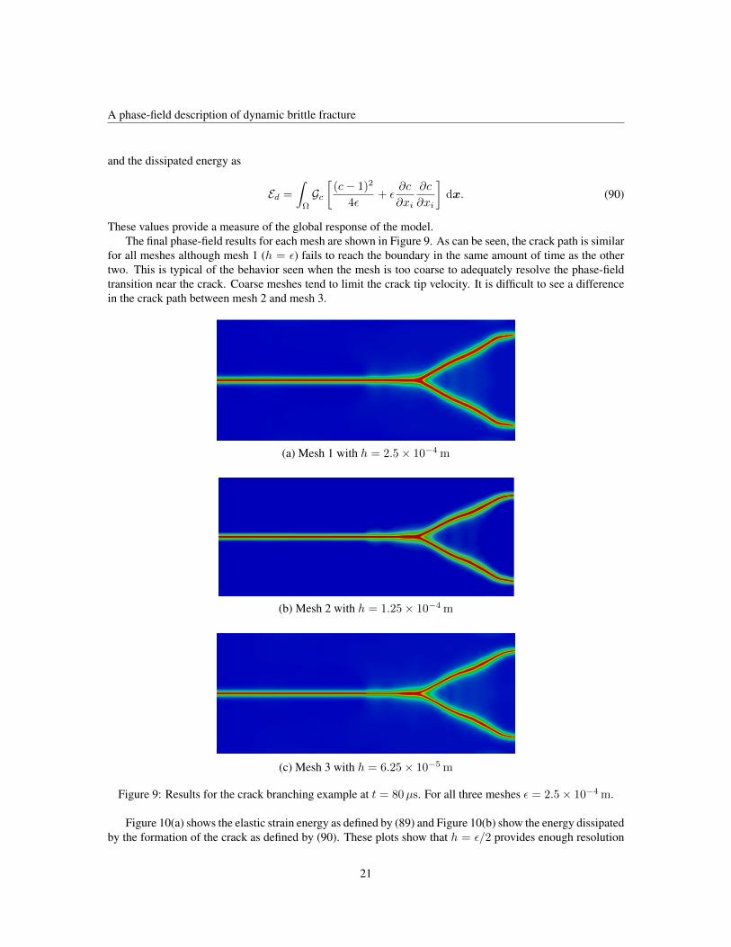
These values provide a measure of the global response of the model.The final phase-field results for each mesh are shown in Figure 9. As can be seen, the crack path is similar

for all meshes although mesh 1 (h = ε) fails to reach the boundary in the same amount of time as the othertwo. This is typical of the behavior seen when the mesh is too coarse to adequately resolve the phase-fieldtransition near the crack. Coarse meshes tend to limit the crack tip velocity. It is difficult to see a differencein the crack path between mesh 2 and mesh 3.

(a) Mesh 1 with h = 2.5× 10−4 m

(b) Mesh 2 with h = 1.25× 10−4 m

(c) Mesh 3 with h = 6.25× 10−5 m

Figure 9: Results for the crack branching example at t = 80µs. For all three meshes ε = 2.5× 10−4 m.

Figure 10(a) shows the elastic strain energy as defined by (89) and Figure 10(b) show the energy dissipatedby the formation of the crack as defined by (90). These plots show that h = ε/2 provides enough resolution

21


to capture the response of the model. For h = ε the mesh is too coarse and the material behaves as if itis too stiff and too much energy is dissipated. This is a result of the mesh being too coarse to capture thegradients of the phase-field near the crack. The crack tip velocity is plotted in Figure 10(c). In all cases, thevelocity stays well below 60% of the Rayleigh wave speed as has been commonly observed in experiments(see Ravi-Chandar and Knauss (1984)).

0.04

0.16

0.12

0.08

Elas

tic S

train

Ene

rgy

[J]

0 20 806040Time [μs]

0

Mesh 1Mesh 2Mesh 3

0 10 20 30 40 50 60 70 80Time [μs]

Mesh 1Mesh 2Mesh 3

0

0.1

0.4

0.3

0.2

Dis

sipa

ted

Ener

gy [J

]

0.6

0.5

(a) (b)

vR

0.6vR

0 10 20 30 40 50 60 70 80Time [μs]

0

1000

1500

2000

2500

Cra

ck T

ip V

eloc

ity [m

/s]

500

Mesh 1Mesh 2Mesh 3

Crack branchingCrack

widening

(c)

Figure 10: Plots over time of (a) the elastic strain energy as defined by (89), (b) the dissipated fracture energyas defined by (90), and (c) crack tip velocity. After branching, the reported crack tip velocity is that of theupper branch.

In Figure 11 we show a post-processed plot of mesh 2 at t = 70µs. In this figure we have scaled thedisplacements by a factor of 50 and removed areas of the model from the plot where c < 0.05 in order toshow a representation of the cracked geometry.

Remark: For the monolithic time integration scheme the size of ∆t is limited by accuracy and convergence.For the dynamic crack branching example discussed here, choosing a time step such that ∆t ≤ 2h/vRproduced acceptable accuracy. For ∆t = 8h/vR the Newton-Raphson method failed to converge near thetime of the initial crack propagation.

22


Figure 11: A post-processed plot of mesh 2 at t = 70µs. The displacements have been scaled by a factor of50 and areas of model where c < 0.05 have been removed from the plot. Pressure is measured in Pascals.

Remark: Since the crack is not tracked algorithmically, the velocity of the crack tip is measured as a post-processing step. For the values reported here, the location of the crack tip, x, is found on an iso-curve of thephase-field with value 0.25. The velocity is then computed as vn = (xn+1 − xn)/∆t.

23


4.3 Dynamic shear loadingIn this example we model crack initiation and propagation under a dynamic shear load. The model is basedon experimental results reported by Kalthoff and Winkler (1987) and Kalthoff (2000). Previous numericalresults of this problem based on XFEM have been reported by Belytschko et al. (2003), among others, and acomparison of results between XFEM, the element deletion method, and the interelement crack method havebeen reported by Song, Wang, and Belytschko (2008). Numerical results of a similar experiment reportedby Ravi-Chandar (1998) have been reported by Remmers, de Borst, and Needleman (2008) where cohesivesegments have been used to model the crack.

The input geometry and loading conditions for the simulation are shown in Figure 12, where symmetryis employed to reduce the computational cost. In the experiment, the load was applied by firing a projectileat a prenotched specimen. In our simulation we model the case where the projectile was fired with a velocityof 33 m/s by applying the kinematic velocity

v =

tt0v0 t ≤ t0

v0 t > t0(91)

where v0 = 16.5 m/s and t0 = 1µs. A no traction boundary condition is applied to all unspecified sur-faces. We model the geometry using quadratic NURBS basis functions. The initial crack is modeled by adiscontinuity in the geometry in order to introduce a sharp crack tip as in Section 4.1.

100 mm

50 mm75 m

m

100

mm

vsymmetry

Figure 12: The geometry and boundary conditions for the dynamic shear loading example. The crack ismodeled by an actual discontinuity in the mesh with a zero radius crack tip. The load is applied as a velocitycondition that is ramped up from 0 to 16.5 m/s in one microsecond and then held constant for the duration ofthe simulation.

The model parameters are ρ = 8000 kg/m3, E = 190 GPa, ν = 0.3, Gc = 2.213× 104 J/m2, k = 0, andplane strain is assumed. The corresponding dilatational, shear, and Rayleigh wave speeds are vd = 5654 m/s,vs = 3022 m/s, vR = 2803 m/s. The length scale was chosen to be ε = 1.95×10−4 m leading to a maximumuniaxial stress of 1.07 GPa (see Section 2.3.1). The mesh has 1024 × 1024 uniform quadratic elements sothat h ≈ ε/2.

The simulations were performed using the staggered integration scheme described in Section 3.3.2 withthe momentum equation being solved explicitly using the HHT-α method with α = −0.1. A fixed time stepof ∆t = 1.25 × 10−8 was chosen, which is slightly less than 0.9∆tcrit, where the critical time step, ∆tcrit,

24


is computed as

∆tcrit =Ωcrit

ωmax(92)

with ωmax the maximum natural frequency of the momentum equation determined from the undamped eigen-problem and (considering only the undamped case)

HHT-α (see Miranda, Ferencz, and Hughes (1989))

Ωcrit =

√2(γ + 2α(γ − β)

γ + 2α(γ − β)(93)

Explicit generalized-α (see Hulbert and Chung (1996))

Ωcrit =

√12(1 + ρb)3(2− ρb)

10 + 15ρb − ρ2b + ρ3

b − ρ4b

. (94)

The resulting phase-field is shown in Figure 13. Note that, initially, the crack starts to propagate at a largerangle then the angle decreases as the crack propagates. The average angle from the initial crack tip to thepoint where the crack intersects the boundary is somewhat greater than 65. This is in fairly good agreementwith the experimental results, which show the crack propagating at about 70. The velocity of the crack tipis shown in Figure 15. As can be seen, the crack quickly accelerates to a velocity just below 60% of theRayleigh wave speed and maintains this velocity until it decreases as the crack approaches the top surface.Although no crack tip velocity information is reported for the experimental results, this velocity behavior isin good agreement with behavior reported by Ravi-Chandar (1998) for a similar experiment.

In Figure 14 we show a post-processed plot of the model at t = 70µs. In this figure we have scaled thedisplacements by a factor of 5 and removed areas of the model from the plot where c < 0.05 in order to showa representation of the cracked geometry.

Remark: Experience has shown that the action of the phase-field does not effect the critical time step ofthe explicit algorithm. Choosing ∆t ≤ 0.9∆tcrit has proven sufficient to maintain stability and is oftenconservative, i.e, letting ∆t = ∆tcrit often results in a stable time step.

4.4 Adaptive refinement schemeThe length scale parameter, ε, plays two roles in the phase-field model: first, it determines the width of theapproximation to the crack, and second, as shown in Section 2.3.1, it influences the magnitude of the tensilestress required for crack nucleation. Thus, in order to capture fine scale details of a crack, or model materialswith high nucleation stresses, a small value for ε is needed. For example, if the maximum uniaxial shearstress is too low for the dynamic shear loading example in Section 4.3, a secondary crack will nucleate atthe surface opposite the initial crack (see Ravi-Chandar et al. (2000)). Thus, a small value of ε is required toaccurately capture the crack topology for this problem. This in turn requires a fine mesh in areas where thecrack is located.

To efficiently compute with fine meshes, as needed to accurately resolve a crack for small values of ε,we introduce an adaptive refinement scheme. For this scheme we choose the phase-field parameter as aconvenient measure for determining the need for refinement. As has been shown, the gradients of the phase-field are high in an area near the crack. Away from the crack the value of the phase-field stays close to one.By choosing a critical threshold of the phase-field that is higher than the value at which crack nucleation

25


(a) t = 20µs (b) t = 40µs

65º

(c) t = 65µs (d) t = 87µs

Figure 13: Evolution of the crack through time for a uniform 1024 × 1024 quadratic NURBS mesh with1,055,242 control points and ε = 1.95× 10−4 m. The resulting crack propagation angle is somewhat greaterthan 65 and close to the experimentally observed angle of about 70 reported by Kalthoff and Winkler (1987)and Kalthoff (2000).

occurs (c = 0.75) the area near the crack is easily identified. Using a larger value for the critical thresholdresults in a greater area of refinement (we have found c = 0.8 to be a good choice). The adaptive refinementscheme we have developed proceeds as follows:

1. Run the dynamic simulation to some termination point

2. Flag elements where the phase-field is below the critical threshold

3. Refine the flagged elements

4. Rerun the simulation with the locally refined mesh

26


Figure 14: A post-processed plot of the dynamic shear loading example at t = 75µs. The displacements havebeen scaled by a factor of 5 and areas of model where c < 0.05 have been removed from the plot. Pressure ismeasured in Pascals.

0 20 906040Time [μs]

0

3000

2000

1000

Cra

ck T

ip V

eloc

ity [m

/s]

vR

0.6vR

Figure 15: Crack tip velocity for dynamic shear loading example.

5. Repeat steps 2—4 until convergence

4.4.1 Analysis-suitable local refinement of T-splines

A distinguishing feature of T-splines is the presence of T-junctions (hanging nodes) in the mesh. T-junctionsmaintain locality in the context of refinement. This is in contrast with NURBS where all refinement isglobal. A highly localized and efficient refinement algorithm for analysis-suitable T-splines was developed

27


Perform Local

Refinement

Flag Bézier elements Extract refined Bézier mesh

Figure 16: A schematic representation of an adaptive refinement scheme based on T-splines, analysis-suitablelocal refinement, and Bezier extraction.

by Scott et al. (2011). This algorithm avoids introducing superfluous control points, preserves exact geometry,generates smooth nested spaces, and maintains the properties of an analysis-suitable space.

In the context of isogeometric analysis, the adaptive refinement scheme is based on Bezier extraction andanalysis-suitable local refinement as shown schematically in Figure 16. First, the flagged Bezier elements areused to determine the basis functions of the T-spline that will be refined. Analysis-suitable local refinementis then applied to generate the refined set of T-spline basis functions. Bezier extraction is then applied to therefined T-spline to generate the new set of Bezier elements.

We apply this refinement scheme to the dynamic shear loading example from Section 4.3. We start witha coarse initial C2-continuous cubic T-spline that has 128 × 128 Bezier elements. For all meshes, ε is setto 1.95 × 10−4 m. Elements are flagged for refinement if the phase-field parameter is less than 0.8 at anyquadrature point within the element. The sequence of results shown in Figure 17 where each simulation wasterminated at t = 100µs. Figure 18 shows the sequence of meshes with the elements that have been flaggedfor refinement at the end of each iteration. Note that when the mesh is too coarse, the crack propagation isrestricted and the direction is incorrect. It is not until mesh 3, when h = ε, that the mesh is fine enough tocapture the correct crack path.

Figure 19 compares the elastic strain energy and dissipated energy at each refinement iteration to the solu-tion from Section 4.3, which we call the reference solution. The elastic strain energy, shown in Figure 19(a),is over predicted for the coarse meshes as a result of restricted crack propagation. This plot shows that it isnot until mesh 4, when most of the element along the propagation path are such that h = ε/2, that the elasticstrain energy agrees well with the reference solution. This is also true for the dissipated energy shown inFigure 19(b).

Table 2 lists the total number of functions for each mesh in the refinement sequence and the numberof elements that were flagged at the end of each simulation. Note that the final mesh has 53,032 cubic basisfunctions. This is compared to 1,055,242 quadratic basis functions in the uniformly refined reference solutionfrom Section 4.3.

Mesh 1 Mesh 2 Mesh 3 Mesh 4 Mesh 5Number of functions 17,755 19,992 27,032 47,824 53,032

Flagged elements 589 2,001 6,257 1,446 8

Table 2: The number basis functions before refinement and the number of elements that were flagged forrefinement for each mesh.

28


Mesh 1 Mesh 2 Mesh 3

Mesh 4 Mesh 5

Figure 17: Kalthoff mesh refinement results. Mesh 1 is a 128 x 128 cubic T-spline mesh. Bezier elementswere flagged for refinement if c < 0.8 at any quadrature point inside the element and h =

√a > 1.94 ×

10−4 m where a is the element area.

29


Mesh 1 Mesh 2

Mesh 3 Mesh 4

Figure 18: The first four meshes in the local refinement sequence. The elements in red are those that wereselected to be refined at each step.

30


ReferenceMesh 1Mesh 2Mesh 3Mesh 4Mesh 5

Time, [μs]0 20 40 60 80

0

2000

4000

6000

Elas

tic S

train

Ene

rgy

[J]

ReferenceMesh 1Mesh 2Mesh 3Mesh 4Mesh 5

Time, [μs]0 20 40 60 80

0

2000

4000

6000D

issi

pate

d En

ergy

[J]

(a) (b)

Figure 19: The (a) elastic strain energy,∫

Ω[(1 − k)c2 + k]ψ+

e + ψ−e dx, and (b) dissipated energy,∫ΩGc[(c− 1)2/(4ε) + ε|∇c|2

]dx, for the sequence of refined meshes shown in Figure 17. The reference

mesh is the uniformly refined mesh from Figure 13.

31


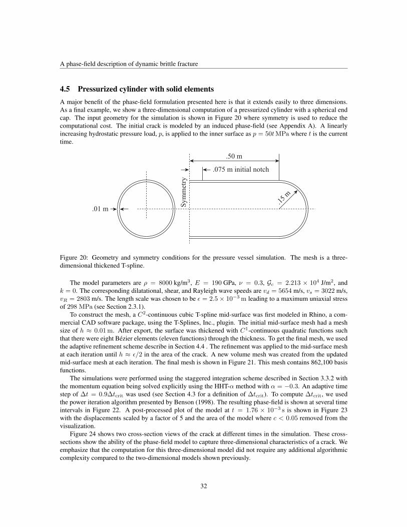
4.5 Pressurized cylinder with solid elementsA major benefit of the phase-field formulation presented here is that it extends easily to three dimensions.As a final example, we show a three-dimensional computation of a pressurized cylinder with a spherical endcap. The input geometry for the simulation is shown in Figure 20 where symmetry is used to reduce thecomputational cost. The initial crack is modeled by an induced phase-field (see Appendix A). A linearlyincreasing hydrostatic pressure load, p, is applied to the inner surface as p = 50tMPa where t is the currenttime.

.50 m

Sym

met

ry

.075 m initial notch

.01 m .1

5 m

Figure 20: Geometry and symmetry conditions for the pressure vessel simulation. The mesh is a three-dimensional thickened T-spline.

The model parameters are ρ = 8000 kg/m3, E = 190 GPa, ν = 0.3, Gc = 2.213 × 104 J/m2, andk = 0. The corresponding dilatational, shear, and Rayleigh wave speeds are vd = 5654 m/s, vs = 3022 m/s,vR = 2803 m/s. The length scale was chosen to be ε = 2.5× 10−3 m leading to a maximum uniaxial stressof 298 MPa (see Section 2.3.1).

To construct the mesh, a C2-continuous cubic T-spline mid-surface was first modeled in Rhino, a com-mercial CAD software package, using the T-Splines, Inc., plugin. The initial mid-surface mesh had a meshsize of h ≈ 0.01 m. After export, the surface was thickened with C1-continuous quadratic functions suchthat there were eight Bezier elements (eleven functions) through the thickness. To get the final mesh, we usedthe adaptive refinement scheme describe in Section 4.4 . The refinement was applied to the mid-surface meshat each iteration until h ≈ ε/2 in the area of the crack. A new volume mesh was created from the updatedmid-surface mesh at each iteration. The final mesh is shown in Figure 21. This mesh contains 862,100 basisfunctions.

The simulations were performed using the staggered integration scheme described in Section 3.3.2 withthe momentum equation being solved explicitly using the HHT-α method with α = −0.3. An adaptive timestep of ∆t = 0.9∆tcrit was used (see Section 4.3 for a definition of ∆tcrit). To compute ∆tcrit, we usedthe power iteration algorithm presented by Benson (1998). The resulting phase-field is shown at several timeintervals in Figure 22. A post-processed plot of the model at t = 1.76 × 10−3 s is shown in Figure 23with the displacements scaled by a factor of 5 and the area of the model where c < 0.05 removed from thevisualization.

Figure 24 shows two cross-section views of the crack at different times in the simulation. These cross-sections show the ability of the phase-field model to capture three-dimensional characteristics of a crack. Weemphasize that the computation for this three-dimensional model did not require any additional algorithmiccomplexity compared to the two-dimensional models shown previously.

32


Figure 21: The final mesh for the pressurized cylinder example problem. The volumetric mesh was con-structed by thickening a mid-surface mesh. The refinement was performed using the adaptive refinementscheme describe in Section 4.4 which resulted in a final mesh containing 862,100 basis functions.

Remark: This model demonstrates several key features of isogeometric analysis. First, the initial mid-surface model was constructed in a commercial CAD software package. This model was used directly toconstruct the analysis model, i.e., there is no intermediate meshing step. Second, the smoothness of the CADgeometry is represented exactly by the analysis model. Finally, refinement was performed directly on theCAD model and the exact CAD geometry was maintained at each iteration. This is illustrated in Figure 21.

33


(a) t = 1.02× 10−3 s (b) t = 1.38× 10−3 s

(c) t = 1.53× 10−3 s (d) t = 1.76× 10−3 s

Figure 22: The results of the pressurized cylinder example. The phase-field is shown.

34


Figure 23: A post-processed plot of the pressure vessel example at t = 1.76 × 10−3 s. The displacementshave been scaled by a factor of 5 and areas of model where c < 0.05 have been removed from the plot.Displacement is measured in meters.

t = 1.02×10-3 s

t = 1.53×10-3 s

Figure 24: Cross section views showing the three-dimensional phase-field profiles of the crack surfaces.

35


5 ConclusionWe have extended the phase-field model for quasi-static brittle fracture presented by Miehe, Hofacker, andWelschinger (2010a) to the dynamic case. The phase-field model provides a smooth representation of a crackand removes the requirement to numerically track discontinuities in the displacement field. The width ofthe phase-field approximation of a discrete crack is controlled by a length scale parameter. We have shownthat this parameter also influences the critical stress at which crack nucleation occurs and should therefore beconsidered as a material parameter. To perform time integration of the dynamic model, we have presentedboth a monolithic and a staggered time integration scheme. The staggered scheme provides efficiency andflexibility in how the momentum equation is integrated and therefore holds greater potential for large three-dimensional problems.

We have studied the behavior of the model by performing numerical experiments for crack propaga-tion and branching. These examples have shown that the phase-field model can accurately capture complexdynamic crack propagation behavior in both two and three dimensions. In addition, we have proposed anadaptive local refinement strategy that allows for the efficient simulation of complex crack patterns. This re-finement strategy takes advantage of the character of the phase-field evolution to determine when refinementis needed. We have demonstrated by numerical examples the effectiveness of this refinement scheme in thecontext of T-spline-based isogeometric analysis.

As a finally example, we have shown that the combination of the phase-field model and local refinementstrategy provides an effective method for simulating fracture in three-dimensional structures. The abilityto simply and effectively model three-dimensional fracture is perhaps the most significant attribute of thephase-field model.

AcknowledgementsThis work was supported by grants from the Office of Naval Research (N00014-08-1-0992), the ArmyResearch Office (W911NF-10-1-0216 ), the National Science Foundation (CMI-0700807), and SINTEF(UTA10-000374). M. A. Scott was partially supported by an ICES CAM Graduate Fellowship. M. J. Bordenwas partially supported by Sandia National Laboratories. Sandia is a multiprogram laboratory operated bySandia Corporation, a Lockheed Martin Company, for the United States Department of Energy’s NationalNuclear Security Administration under contract DE-AC04-94AL85000. This support is gratefully acknowl-edged.

The authors also acknowledge the Texas Advanced Computing Center (TACC) at The University of Texasat Austin for providing HPC and visualization resources that have contributed to the research results reportedwithin this paper. URL: http://www.tacc.utexas.edu

A Modeling a preexisting crack in a continuous bodyFor the numerical examples discussed in this paper, a preexisting crack is used to initialize crack propagation.The initial crack is model as either a discrete crack in the geometry or as an induced crack in the phase-field.For the induced crack, an initial strain-history field is specified such that an initial crack in the phase-field isdefined. To define the initial strain-history field we let l be a line that represents the discrete crack we wishto include and d(x, l) is the closest distance from x to the line l. The strain-history field is then defined as

H0(x) = B

Gc4ε

(1− d(x,l)

ε

)d(x, l) ≤ ε

0 d(x, l) > ε(95)

36


where the magnitude of the scalar B can be determined by letting d = 0 and substituting H0 into (12)2 withk = 0 and ∂2c/∂xi = 0 to get

B =1

c− 1. (96)

In the examples presented above, we have chosen c = 10−3 to be the value of the phase-field in the initialcrack so that B = 103.

B Dimensionless form of the phase-field equationsTo improve the conditioning and scaling of the fully coupled system of equations discussed in Section 3.3.1,we consider the strong form equations (12) in their dimensionless form. To arrive at the dimensionlessformulation we define a length scale L0 and time scale T0 as

L0 =GcChE

, T0 = L0

√ρ

ChE(97)

where the non-dimensional constant Ch is used to control the scaling of the problem. By introducing non-dimensional space and time coordinates, and a non-dimensional displacement field as

x∗ = x/L0, t∗ = t/T0, u∗ = u/L0 (98)

we arrive at

∂σ∗ij∂x∗j

=∂2u∗i∂(t∗)2

[4ε∗(1− k)H∗ + 1] c− 4(ε∗)2 ∂2c

∂(x∗i )2

= 1

(99)

withσ∗ =

σ

ChE, H∗ =

HChE

, ε∗ =ε

L0(100)

In practice, we have found that choosing Ch such that the size of the elements in the mesh have an area equalto one yields good results.

Remark: The same implementation can be used to compute with both the dimensional and non-dimensionalforms of the equations. If the dimensional form of the equations has been implemented then the non-dimensional form can be computed by setting the material parameters Gc = 1, ρ = 1, and E = 1/Ch;scaling the input geometry by 1/L0; scaling the time steps by 1/T0; and using ε∗ in place of ε.

ReferencesL. Ambrosio and V. M. Tortorelli. Approximation of functional depending on jumps by elliptic functional

via Γ-convergence. Communications on Pure and Applied Mathematics, 43(8):999–1036, 1990.

I. Babuska and J. M. Melenk. The partition of unity method. International Journal for Numerical Methodsin Engineering, 40(4):727–758, 1997.

37


T. Belytschko, H. Chen, J. Xu, and G. Zi. Dynamic crack propagation based on loss of hyperbolicity anda new discontinuous enrichment. International Journal for Numerical Methods in Engineering, 58(12):1873–1905, 2003.

D. J. Benson. Stable time step estimation for multi-material eulerian hydrocodes. Computer Methods inApplied Mechanics and Engineering, 167(1-2):191–205, 12 1998.

D. J. Benson, Y. Bazilevs, M. C. Hsu, and T. J. R. Hughes. A large deformation, rotation-free, isogeometricshell. Computer Methods in Applied Mechanics and Engineering, 200(13-16):1367–1378, 2011.

M. J. Borden, M. A. Scott, J. A. Evans, and T. J. R. Hughes. Isogeometric finite element data structures basedon Bezier extraction of NURBS. International Journal for Numerical Methods in Engineering, In press:DOI: 10.1002/nme.2968, 2010.

B. Bourdin, G. A. Francfort, and J. J. Marigo. The variational approach to fracture. Journal of Elasticity, 91(1-3):5–148, April 2008.

B. Bourdin, C. Larsen, and C. Richardson. A time-discrete model for dynamic fracture based on crackregularization. International Journal of Fracture, 168(2):133–143, 2011.

J. Chung and G. M. Hulbert. A time integration algorithm for structural dynamics with improved numericaldissipation: The generalized-alpha method. Journal of Applied Mechanics, 60(2):371–375, 1993.

H. M. Hilber, T. J. R. Hughes, and R. L. Tayler. Improved numerical dissipation for time integration algo-rithms in structural dynamics. Earthquake Engineering and Structural Dynamics, 5:283–292, 1977.

T. J. R. Hughes. The Finite Element Method: Linear Static and Dynamic Finite Element Analysis. DoverPublications, Mineola, NY, 2000.

T. J. R. Hughes, J. A. Cottrell, and Y. Bazilevs. Isogeometric analysis: CAD, finite elements, NURBS,exact geometry and mesh refinement. Computer Methods in Applied Mechanics and Engineering, 194:4135–4195, 2005.

T. J. R. Hughes, A. Reali, and G. Sangalli. Duality and unified analysis of discrete approximations in struc-tural dynamics and wave propagation: Comparison of p-method finite elements with k-method NURBS.Computer Methods in Applied Mechanics and Engineering, 197(49-50):4104–4124, 2008.

T. J. R. Hughes, A. Reali, and G. Sangalli. Efficient quadrature for NURBS-based isogeometric analysis.Computer Methods in Applied Mechanics and Engineering, 199(5-8):301–313, 2010.

G. M. Hulbert and J. Chung. Explicit time integration algorithms for structural dynamics with optimalnumerical dissipation. Computer Methods in Applied Mechanics and Engineering, 137:175–188, 1996.

J. Kalthoff. Modes of dynamic shear failure in solids. International Journal of Fracture, 101(1):1–31, 2000.

J. F. Kalthoff and S. Winkler. Failure mode transition of high rates of shear loading. In C. Y. Chiem, H. D.Kunze, and L. W. Meyer, editors, Proceedings of the International Conference on Impact Loading andDynamic Behavior of Materials, volume 1, pages 185–195, 1987.

A. Karma, D. A. Kessler, and H. Levine. Phase-field model of mode III dynamic fracture. Physical ReviewLetters, 87(4):045501, 2001.

R. Krueger. Virtual crack closure technique: History, approach, and applications. Applied Mechanics Re-views, 57(2):109–143, 2004.

38


C. J. Larsen. Models for dynamic fracture based on griffith’s criterion. In K. Hackl, editor, IUTAM Symposiumon Variational Concepts with Applications to the Mechanics of Materials, volume 21, pages 131–140.Springer Netherlands, 2010.

C. J. Larsen, C. Ortner, and E. Suli. Existence of solutions to a regularized model of dynamic fracture.Mathematical Methods and Models in Applied Sciences, 20(7):1021–1048, 2010.

X. Li, J. Zheng, T. W. Sederberg, T. J. R. Hughes, and M. A. Scott. On the linear independence of T-splines. Computer Aided Geometric Design, submitted for publication (see also ICES Report 10-40 athttp://www.ices.utexas.edu/research/reports), 2010.

C. Miehe, M. Hofacker, and F. Welschinger. A phase field model for rate-independent crack propagation:Robust algorithmic implementation based on operator splits. Computer Methods in Applied Mechanicsand Engineering, 199(45-48):2765–2778, 2010a.

C. Miehe, F. Welschinger, and M. Hofacker. Thermodynamically consistent phase-field models of fracture:Variational principles and multi-field fe implementations. International Journal for Numerical Methods inEngineering, 83(10):1273–1311, 2010b.

I. Miranda, R. M. Ferencz, and T. J. R. Hughes. An improved implicit-explicit time integration method forstructural dynamics. Earthquake Engineering and Structural Dynamics, 18:643–653, 1989.

N. Moes, J. Dolbow, and T. Belytschko. A finite element method for crack growth without remeshing.International Journal for Numerical Methods in Engineering, 46(1):131–150, 1999.

D. Mumford and J. Shah. Optimal approximations by piecewise smooth functions and associated variationalproblems. Communications on Pure and Applied Mathematics, 42(5):577–685, 1989.

L. Piegl and W. Tiller. The NURBS Book (Monographs in Visual Communication), 2nd ed. Springer-Verlag,New York, 1997.

K. Ravi-Chandar. Dynamic fracture of nominally brittle materials. International Journal of Fracture, 90(1):83–102, 03 1998.

K. Ravi-Chandar and W. G. Knauss. An experimental investigation into dynamic fracture: III. on steady-statecrack propagation and crack branching. International Journal of Fracture, 26(2):141–154, 1984.

K. Ravi-Chandar, J. Lu, B. Yang, and Z. Zhu. Failure mode transitions in polymers under high strain rateloading. International Journal of Fracture, 101:33–72, 2000.

J. J. C. Remmers, R. de Borst, and A. Needleman. The simulation of dynamic crack propagation using thecohesive segments method. Journal of the Mechanics and Physics of Solids, 56(1):70–92, 1 2008.

M. A. Scott, M. J. Borden, C. V. Verhoosel, and T. J. R. Hughes. Isogeometric finite element data structuresbased on bezier extraction of T-splines. International Journal for Numerical Methods in Engineering, inpress, doi: 10.1002/nme.3167, 2010.

M. A. Scott, X. Li, T. W. Sederberg, and T. J. R. Hughes. Local refinement of analysis-suitable T-splines.Computer Methods in Applied Mechanics and Engineering, submitted for publication (see also ICES Re-port 11-06 at http://www.ices.utexas.edu/research/reports), 2011.

S.-H. Song, H. Wang, and T. Belytschko. A comparative study on finite element methods for dynamicfracture. Computational Mechanics, 42(2):239–250, July 2008.

39


C. V. Verhoosel, M. A. Scott, R. de Borst, and T. J. R. Hughes. An isogeometric approach to cohesive zonemodeling. International Journal for Numerical Methods in Engineering, To appear, 2010.

C. V. Verhoosel, M. A. Scott, T. J. R. Hughes, and R. de Borst. An isogeometric analysis approach to gradientdamage models. International Journal for Numerical Methods in Engineering, 86(1):115–134, 2011.

40

ices report 11-14 - university of texas at austin

Documents