ICF CONSULTING 1

______________________________________________________________________________________010108 Final - January 2001

Final Report

DEVELOPMENT AND IMPLEMENTATION OF A HOMOLOGY MAPPINGTECHNIQUE TO AID THE SELECTION OF CITIES FOR MODELING OF THE

EFFECTS OF URBAN HEAT ISLAND MITIGATION MEASURES ON OZONE AIRQUALITY

SYSAPP-01-008

31 January 2001

Prepared for

Mr. Edgar MercadoGlobal Programs Division

U.S. Environmental Protection AgencyAriel Rios Building (6205J)

1200 Pennsylvania Avenue, NWWashington, D.C. 20460

Prepared by

Sharon G. DouglasA. Belle Hudischewskyj

Jeffrey R. LundgrenICF Consulting/

Systems Applications International, Inc.101 Lucas Valley Road

San Rafael, California 94903

2 ICF CONSULTING

______________________________________________________________________________________0101008 Final – January 2001

Copyright 2001 by Systems Applications International, Inc.

ICF CONSULTING 3

______________________________________________________________________________________010108 Final - January 2001

Contents

1 INTRODUCTION…………………………………………………… 5

2 HOMOLOGY MAPPING TECHNIQUE…………………………… 7Overview…………………………………………………………….. 7Application Procedures……………………………………………… 8

3 RESULTS FOR METEOROLOGICAL MODELING……………… 17

4 RESULTS FOR PHOTOCHEMCIAL MODELING……………….. 21Discussion of Methodology…………………………………………. 21Recommendations…………………………………………………… 22

References…………………………………………………………………… 29

4 ICF CONSULTING

______________________________________________________________________________________0101008 Final – January 2001

ICF CONSULTING 5

______________________________________________________________________________________010108 Final - January 2001

1 INTRODUCTION

This report summarizes the application of a homology mapping technique to aid the selection ofcities for photochemical modeling – the purpose of which is to assess the effects of Heat IslandReduction Initiative (HIRI) measures on ozone air quality.

An urban heat island occurs when the temperature within a city is warmer than the surroundingarea. It is an example of inadvertent climate modification (Oke, 1978). Higher temperatureswithin an urban area have the potential to adversely influence ozone air quality through highertemperatures, faster photochemical reaction rates, and greater emissions. Thus, EPA isinvestigating the effectiveness of urban heat island reduction as an ozone mitigation strategy.Two measures that have been identified as part of the EPA program to be potentially effective inreducing the high temperatures associated with an urban heat island are (1) use of reflective roofand paving material to increase the reflectivity or “albedo” of an urban area and (2) increasedvegetation cover (e.g., tree planting).

Before such measures can be reliably implemented, however, it is necessary to carefully examineboth the direct and indirect effects that may influence or alter the complex interactions amongthe various meteorological, emissions, and air quality parameters participating in the formationand transport of ozone. These effects may be beneficial or disbenficial to ozone concentrationlevels, and thus the combined total effects (including “side effects”) must be considered. Forexample, by altering the surface energy budget, a higher albedo will affect other meteorologicalparameters such as wind speed, effective mixing height, and specific humidity. Lower mixingheights resulting from the lower temperatures may offset air quality benefits derived from thereduced chemical reaction rates. Conversely, increased vegetation cover (shading) will alsoresult in lower surface temperatures, and increased roughness lengths associated with thevegetation may enhance the atmospheric mixing processes. Lower temperatures will reduce theproduction of biogenic hydrocarbon emissions from existing vegetation and enhance thedeposition of ozone and other pollutant species, but the addition of vegetation may offset thiseffect. Lower surface temperatures may also reduce emissions from motor vehicles (inparticular, evaporative emissions) and power plants (due to reduced energy demand for cooling).

Meteorological and air quality models can be used to represent the complex interactions betweenland-use, meteorology, emissions, and ozone formation and transport processes, and to estimatethe effects of the HIRI measures on temperature and other meteorological parameters as well asozone air quality. As part of an ongoing study sponsored by the Global Programs Division, EPAis conducting modeling to examine the potential air quality benefits from HIRI measures forselected cites throughout the U.S.

A detailed modeling analysis to assess the effectiveness of HIRI measures involves thecompilation of meteorological and air quality data and preparation of a variety of modelinginputs, as well as the application of urban-/or regional scale meteorological and photochemicalmodeling tools. The modeling process is time and resource intensive and, thus, a detailedmodeling analysis for every U.S. city that could potentially benefit from implementing HIRImeasures is not likely. Thus, EPA has elected to conduct detailed, state-of-the-science modeling

6 ICF CONSULTING

______________________________________________________________________________________0101008 Final – January 2001

of selected cites and to examine the feasibility of using the results from these selected cities torepresent (either qualitatively or quantitatively) the meteorological and/or ozone air qualityresponse to HIRI measures for other not-modeled cities.

To this end, selection of cities that are “prototypical” and might best be used to represent othercities may enhance or extend the utility of the modeling exercise/results. An approach to cityselection that is based on a homology mapping technique is presented in this report.

Homology mapping is a technique in which similarities in the geographical, land-use, andmeteorological characteristics of a monitoring site or, in this case, urban area are used to identifya homologue or best match (from a list of surrogates) for that site or area. This technique wasdeveloped to map observed ozone data (for actual monitoring sites) to unmonitored areas (orpseudo monitoring sites) as part of the EPA-sponsored Section 812 prospective modelinganalysis (designed to examine the costs and benefits of the Clean Air Act Amendments of 1990)– to provide the basis for health effects calculations throughout the U.S. (in both monitored andunmonitored areas). This application of the technique is described by Iwamiya and Douglas,1999).

Homology mapping was used in this study to identify urban areas that could be used to representother urban areas with respect to (1) meteorological response and (2) ozone air quality responseto implementing HIRI measures. The idea is that if detailed modeling can only be done for alimited number of areas, choosing areas for modeling that are representative of other areas mayextend the utility of the modeling results.

The remainder of this report summarizes the methods and results of the homology mappingbased city selection analysis. Recommendations for approximately 25, 15, and 10 cities orcombined urban areas representing various distributions of severity of ozone air quality problemare provided. Design of modeling domains that would capture the ten cities option is alsodiscussed.

ICF CONSULTING 7

______________________________________________________________________________________010108 Final - January 2001

2 HOMOLOGY MAPPING TECHNIQUE

In this section, we present an overview of the homology mapping concept/technique and thenpresent the application procedures used for the HIRI analysis.

OVERVIEW

Homology mapping is based on the assumption that urban areas with similar characteristics (e.g.,geographical, land-use, emissions, and population) will also share other characteristics (e.g.,meteorological conditions, air quality) – provided that the latter set is determined by the formerand the controlling characteristics can be identified and represented quantitatively. Homologymapping can be used to map or assign “data” from one area to another (where “data” can take theform of observed values or modeling results). Mapping for each area of interest is determined byfinding the best match among a set of selected areas, of the factors believed to influence the localconditions. With respect to meteorological and ozone air quality conditions, such factors mayinclude the proximity and size of nearby cities, distance to nearest body of water, land usecharacteristics, and latitude. For each area of interest these factors are combined to form ageographical information system or “GIS” vector. Comparison of the vector quantities is thenused to determine the best match. In general, the homology mapping approach includes foursteps:

• Identifying the areas of interest

• Identifying the factors expected to influence the conditions to be represented (e.g. localmeteorology, ozone concentration level, response to changing conditions)

• Creating the GIS vectors

• Finding the best match

The first two steps are specific to the application and are discussed in more detail in thefollowing section. A general description of the mathematical components of the vector creationand comparison (finding the best match) steps is given here.

Once the GIS elements are established and requisite data are compiled, each GIS vector(representing a particular urban area) will include numerous components. In addition, some ofthe vector components may also have subcomponents. Each of these may have different unitsand/or ranges – so the final step in creating the GIS vectors is to standardize the components.The individual components of the vectors are standardized based upon the mean and standarddeviation for the components of the GIS vectors.

where

−•

=Χ

i

ii

ii std

meanxN

)(1

8 ICF CONSULTING

______________________________________________________________________________________0101008 Final – January 2001

Xi - Standardized value for vector component iNi - Number of components in sub-vector group for component ixi - Actual value for vector component imeani - Mean of vector component i for monitor GIS vectors onlystdi - Standard deviation of vector component i for monitor GIS vectors only

In essence, a z score is calculated for each of the individual components of the GIS vectors.Each standardized component for the GIS vectors now has a mean of zero and a standarddeviation of one. The value for each of the standardized components is then divided by thenumber of subcomponents for the corresponding vector component. This procedure is necessarybecause of the differing units and scales of the components. Without standardization, certaincomponents would have more weight than others.

Once the vectors are standardized, suitable matches are identified by calculating and comparingthe Euclidean distance between each area under consideration. The Euclidean distance is definedas follows:

{Xarea1,i} - Standardized GIS vector for a given area{Xarea2,i} - Standardized GIS vector for another area

This method for associating two urban areas minimizes the Euclidean distance between the GISvectors, not the physical distance between the two areas. The smaller the value of Euclideandistance, the better the match. The best, second, and third best possible pairings are identified.

APPLICATION PROCEDURES

For the HIRI analysis, homology mapping was used in two ways. First to identify urban areasthat are expected to have similar meteorological features and second to identify areas that areexpected to have similar ozone air quality characteristics. By determining the matches based onthe controlling or influencing factors, rather than simply the observed characteristics (e.g.,temperature, ozone design value1) it is expected that the matches can be used to estimate theeffects of changes due to implementation of HIRI measures (a causal relationship can beestablished).

The approach generally follows the methodology developed for the 812 project but was modifiedto accommodate cities rather than monitoring sites. Overall, however, the idea is the same – touse simulation results for modeled cities to represent the same for cities that are not modeled. Inthis case, simulation results could refer to one of two things: 1) simulated changes inmeteorological parameters (e.g., temperature, effective mixing height, moisture, etc.) from a

1 Ozone design value is a multi-year representation of ozone concentration levels within an urban area.

21, 2,( 1, 2) ( )area i area i

i

DistEuclidean area area = Χ − Χ∑

ICF CONSULTING 9

______________________________________________________________________________________010108 Final - January 2001

meteorological model (e.g., MM52) due to incorporation of HIRI measures or 2) simulated ozoneconcentration changes from a photochemical model (e.g., UAM-V3) due to incorporation ofHIRI measures. These correspond to different levels in EPA’s proposed streamlining approach(to accounting for the effects of heat island reduction).

Step 1: Select Urban Areas

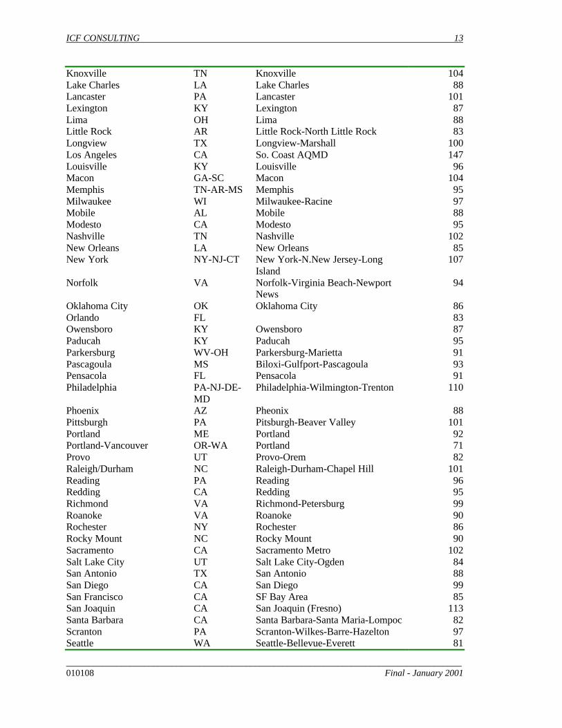
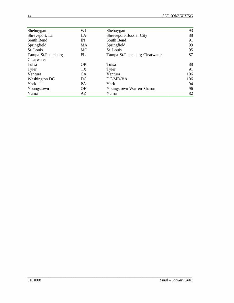
In determining which areas to include in this analysis, we obtained the current (1997-1999) 8-hour ozone design values for all areas in the U.S. from “The Green Book” on the EPA web siteand selected all areas for which the design value is equal to or greater than the expected 8-hourozone standard of 85 ppb. In addition, other areas with somewhat lower design values thatrepresent large population centers were also included. The 8-hour design value is currentlydefined as the three-year average of the fourth highest annual ozone concentration. It iscalculated for each monitoring site and the maximum among all monitoring sites within an urbanarea is used to characterize the area. The list of urban areas used for this analysis and theirdesign values are given in Table 2-1.

Step 2: Determine “GIS” Vector Elements

The next step in setting up a homology map is to identify important geographical, population,emissions, and air quality related values that can be represented quantitatively and used todescribe features that are important to or are likely to influence 1) and 2) above. For thisanalysis, we included:

1. Latitude2. Elevation3. Distance to the nearest body of water4. Land use5. Population6. Area (areal extent)7. Population density8. Population distance of nearby cities9. Emissions-based VOC/NOx ratio10. 8-hour ozone design value

We also considered other parameters such as amount of solar insolation (annual or seasonal),average temperature, number of heating degree days, and amount of urban biogenic emissions.However, these should be represented by those on the list above (i.e., latitude, distance to thenearest body of water, and elevation will largely determine the amount of solar insolation andtemperature; land-use will determine the amount of biogenic emissions, etc.).

The vector components were designed to capture the basic geophysical features that can be usedas surrogates for the physical and chemical processes that govern the formation, transport, and 2 The Pennsylvania State University/National Center for Atmospheric Research (PSU/NCAR) Mesoscale Model,Version 53 The variable-grid Urban Airshed Model developed by Systems Applications International, Inc.

10 ICF CONSULTING

______________________________________________________________________________________0101008 Final – January 2001

deposition of ozone, and result in geographical differences in ozone concentration. The designand construction of the vectors is described in the following paragraphs.

The latitude component is simply the latitude of the urban area. Similarly elevation is elevationabove sea level. The latitude and elevation vector components are important in determiningmeteorology and surrogates for both photolysis rate and temperature, important determinants ofozone production and precursor emission rates.

The distance to nearest body of water was calculated using gridded land-use data (described inmore detail below). It is the distance from the center of the urban area to the nearest large bodyof water. Proximity to water will influence the temperature and horizontal and verticaldispersion characteristics of an area.

The land-use vector component provides information related to processes that influence both theproduction and the deposition of ozone. Land use influences (or in some cases is influenced by)both the meteorology of an area and the amount and density of anthropogenic and biogenicemissions. Deposition velocities (which determine the rate at which ozone and precursorpollutants are taken out of the atmosphere through deposition onto the surface) are also land-usedependent. For example, deposition of ozone is much more rapid over forested areas than watersurfaces. This is also likely an important determinant in the effectiveness of HIRI measures.

The land-use components were estimated using gridded U.S. Geological Survey (USGS) land-use data. Eleven components describe the percentage of area that is urban, agricultural, range,deciduous forest, coniferous forest (including wetlands), mixed forest, water, barren land, non-forest wetlands, mixed agricultural and range, and rocky (low shrubs).

Population, area, and population density were based on 1990 U.S. Census Bureau informationand may help to characterize both the amount and distribution of anthropogenic emissions (e.g.,from motor vehicles) as well as the existence and magnitude of an urban heat island.

The population-distance vector component was designed to capture the influence of neighboringpopulation centers upon the ambient concentrations of ozone. Both the size and proximity ofthese population centers have the potential to influence ambient concentrations. Largerpopulation centers will generally produce more precursor pollutants to ozone formation. Due tothe limiting effects of pollutant transport and diffusion, the proximity to such population centersis a primary consideration. To accommodate the prevailing westerly wind directions, onlywestward population distance was considered.

The westward population-distance components were constructed by first compiling a list of23,655 cities, towns, military bases, etc. and dividing these into deciles, based on population.Again population estimates were based on 1990 U.S. Census data. Those places withpopulations greater than the first decile were retained and counted if they were within 50, 100, or200 km of an urban area. In this manner, 27 components of the westward population-distancesub-vector were constructed. Only those places lying to the west of the urban area. Thedirectional determination was based on longitude and therefore includes the southwest, west, andnorthwest directions.

ICF CONSULTING 11

______________________________________________________________________________________010108 Final - January 2001

The VOC-to-NOx ratio was based on a national-scale emissions inventory (ca. 2000) developedfor photochemical modeling under another EPA work assignment. The emissions were extractedfor the grid-cell or grid-cells encompassing the urban area and the ratio was calculated. Thisratio determines the response of ozone to changes in emissions.

A subset of these components (1 through 4) was used to find homologues for meteorologicalmodeling. All of the components listed above were used for the companion analysis forphotochemical modeling.

Step 2: Set Up GIS Vectors

The next step was to prepare the electronic files that contain the GIS vector element information.This GIS vector elements were standardized using the procedures outlined earlier in this section.

Step 3: Testing and Application of the Homology Mapping Technique

After standardization of the vectors – the homology mapping program/algorithm was designed tomatch each city in a list of not-modeled cities with a corresponding city from a list of themodeled cities. It does this by calculating the Euclidean distance (difference) between the vectorelements and identifies the best match as corresponding to the pair with the smallest distancevalue (difference). It provides a list of the best three matches.

For the HIRI project, we don’t yet know the list of not-modeled and modeled cities. Indeed theobjective of the task is to identify appropriate “prototype” cities for modeling. Accordingly, theapproach was as follows:

1. Select a handful of cities and make sure that they are their own best match (for testingpurposes only)

2. Remove each city one at a time from the “all cities” list and find the best match for each.From the list of three best matches for each city, see if there are any cities that are goodmatches for a number of others (i.e., count the number of times each appears in the top threelist).

These steps were applied twice – once for use with meteorological modeling and once for usewith photochemical modeling – using different sets of GIS vectors (as specified above).

12 ICF CONSULTING

______________________________________________________________________________________0101008 Final – January 2001

Table 2-1. Urban areas used for homology mapping.City State MSA/CMSA/AREA 8-hr Ozone

Design value

Allentown PA Allentown-Bethlehem-Easton 100Altoona PA Altoona 95Asheville NC Asheville 94Atlanta GA Atlanta, 118Augusta GA Augusta-Aiken 92Austin TX Austin-San Marcos 88Baltimore MD Baltimore 109Baton Rouge LA Baton Rouge 92Beaumont-Port Arthur TX Beaumont-Port Arthur 88Benton Harbor MI Benton Harbor 96Birmingham AL Birmingham 97Boston MA Boston-Worcester-Lawrence 95Buffalo NY Buffalo-Niagara Falls 86Canton OH Canton-Massillon 91Charleston WV Charleston 90Charlotte NC Charlotte-Gastonia-Rock Hill 104Chattanooga TN Chattanooga 94Chicago IL-IN Chicago-Gary-Lake Co 93Cincinnati-Hamilton OH Cincinnati 95Clarksville KY Clarksville-Hopkinsville 86Cleveland OH Cleveland-Lorain-Elyria-Akron 99Columbia SC Columbia 92Columbus OH Columbus 97Dallas TX Dallas-Fort Worth 101Dayton OH Dayton-Springfield 94Detroit MI Detroit-Ann Arbor 95Erie PA Erie 93Evansville IN Evansville-Henderson 94Fayetteville NC Fayetteville 92Fort Wayne IN Fort Wayne 88Goldsboro NC Goldsboro 85Grand Rapids MI Grand Rapids-Muskegon-Holland 94Green Bay WI Green Bay 97Greensboro NC Greensboro-Winston-Salem 98Greenville SC Greenville-Spartanburg-Anderson 95Hancock ME Hancock 89Harrisburg PA Harrisburg-Lebanon-Carlisle 97Hartford CT Greater Connecticut 103Hickory NC Hickory-Morganton-Lenoir 90Houston/GAL/Braz. TX Houston/GAL/Braz. 118Huntington-Ashland WV Huntington-Ashland 95Huntsville AL Huntsville 90Indianapolis IN Indianapolis 97Johnson City TN Johnson City-Kingsport-Bristol 91Johnstown PA Johnstown 93Kansas City MO Kansas City 91

ICF CONSULTING 13

______________________________________________________________________________________010108 Final - January 2001

Knoxville TN Knoxville 104Lake Charles LA Lake Charles 88Lancaster PA Lancaster 101Lexington KY Lexington 87Lima OH Lima 88Little Rock AR Little Rock-North Little Rock 83Longview TX Longview-Marshall 100Los Angeles CA So. Coast AQMD 147Louisville KY Louisville 96Macon GA-SC Macon 104Memphis TN-AR-MS Memphis 95Milwaukee WI Milwaukee-Racine 97Mobile AL Mobile 88Modesto CA Modesto 95Nashville TN Nashville 102New Orleans LA New Orleans 85New York NY-NJ-CT New York-N.New Jersey-Long

Island107

Norfolk VA Norfolk-Virginia Beach-NewportNews

94

Oklahoma City OK Oklahoma City 86Orlando FL 83Owensboro KY Owensboro 87Paducah KY Paducah 95Parkersburg WV-OH Parkersburg-Marietta 91Pascagoula MS Biloxi-Gulfport-Pascagoula 93Pensacola FL Pensacola 91Philadelphia PA-NJ-DE-

MDPhiladelphia-Wilmington-Trenton 110

Phoenix AZ Pheonix 88Pittsburgh PA Pitsburgh-Beaver Valley 101Portland ME Portland 92Portland-Vancouver OR-WA Portland 71Provo UT Provo-Orem 82Raleigh/Durham NC Raleigh-Durham-Chapel Hill 101Reading PA Reading 96Redding CA Redding 95Richmond VA Richmond-Petersburg 99Roanoke VA Roanoke 90Rochester NY Rochester 86Rocky Mount NC Rocky Mount 90Sacramento CA Sacramento Metro 102Salt Lake City UT Salt Lake City-Ogden 84San Antonio TX San Antonio 88San Diego CA San Diego 99San Francisco CA SF Bay Area 85San Joaquin CA San Joaquin (Fresno) 113Santa Barbara CA Santa Barbara-Santa Maria-Lompoc 82Scranton PA Scranton-Wilkes-Barre-Hazelton 97Seattle WA Seattle-Bellevue-Everett 81

14 ICF CONSULTING

______________________________________________________________________________________0101008 Final – January 2001

Sheboygan WI Sheboygan 93Shreveport, La LA Shreveport-Bossier City 88South Bend IN South Bend 91Springfield MA Springfield 99St. Louis MO St. Louis 95Tampa-St.Petersberg-Clearwater

FL Tampa-St.Petersberg-Clearwater 87

Tulsa OK Tulsa 88Tyler TX Tyler 91Ventura CA Ventura 106Washington DC DC DC/MD/VA 106York PA York 94Youngstown OH Youngstown-Warren-Sharon 96Yuma AZ Yuma 82

ICF CONSULTING 15

______________________________________________________________________________________010108 Final - January 2001

16 ICF CONSULTING

______________________________________________________________________________________0101008 Final – January 2001

3 RESULTS FOR METEOROLOGICAL MODELING

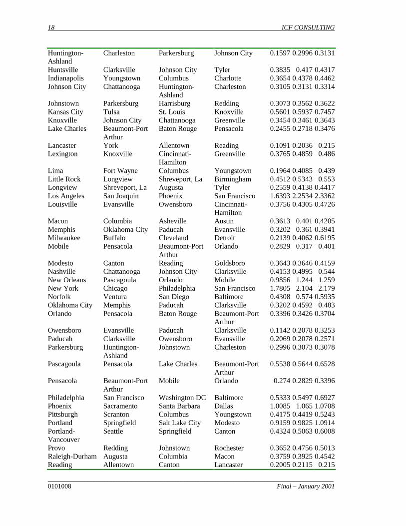
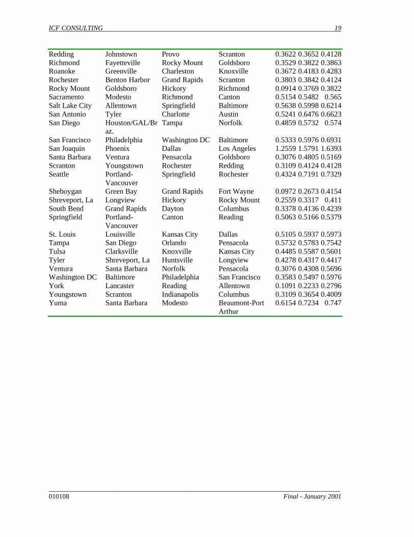
Results of the application of the homology mapping technique to identify urban areas that aremost similar to the greatest number of other urban areas with respect to the meteorologicaldrivers are presented in Table 3-1. For each urban area, the three best matches are given. TheEuclidean distance associated with each match is also provided. While this number has little orno physical meaning, the value can be used to indicate and contrast the relative fidelity of eachmatch.

Urban areas that most frequently appear as matches for other areas include Springfield, IL;Allentown, PA; Beaumont-Port Arthur, TX; Clarksville, WV; Johnson City, TN; Pensacola, FL;Reading, PA; Santa Barbara, CA; Canton, OH; and Chicago, IL. These are the top ten mostfrequent “best-match” areas. They also seem to represent a fairly broad range of geographicareas relative to coastal vs. inland location, latitude, and elevation.

Rather than guide the selection of urban areas for modeling, the meteorological homologues mayprovide the basis for mapping the HIRI meteorological modeling results (in terms of response ofthe meteorological parameters to the HIRI measures). Thus this information is simply presentedhere for possible use later in the HIRI study.

ICF CONSULTING 17

______________________________________________________________________________________010108 Final - January 2001

TABLE 3-1. Homology mapping results for meteorological modeling. ED is Euclidian distance.City Best Match 2nd Best 3rd Best 1st ED 2nd ED 3rd ED

Allentown Reading Lancaster York 0.2005 0.2036 0.2796Altoona Harrisburg Reading Canton 0.3395 0.4633 0.5275Asheville Hickory Macon Shreveport, La 0.3501 0.401 0.4461Atlanta Dallas St. Louis Houston/GAL/Br

az.0.5967 0.6384 0.6901

Augusta Raleigh-Durham Shreveport, La Longview 0.3759 0.412 0.4138Austin Macon Columbia Raleigh-Durham 0.4205 0.566 0.5945Baltimore Washington DC Norfolk Allentown 0.3583 0.5935 0.6011Baton Rouge Beaumont-Port

ArthurLake Charles Pensacola 0.1599 0.2718 0.3407

Beaumont-PortArthur

Baton Rouge Lake Charles Pensacola 0.1599 0.2455 0.274

Benton Harbor Erie Rochester Green Bay 0.3296 0.3803 0.4008Birmingham Longview Greensboro Huntsville 0.4449 0.4469 0.5323Boston Hartford Philadelphia San Francisco 0.6932 0.8528 0.9039Buffalo Milwaukee South Bend Rochester 0.2139 0.5101 0.5329Canton Reading Allentown Modesto 0.2115 0.3158 0.3643Charleston Huntington-

AshlandParkersburg Johnson City 0.1597 0.3078 0.3314

Charlotte Greenville Indianapolis Roanoke 0.4444 0.4462 0.4745Chattanooga Johnson City Knoxville Nashville 0.3105 0.3461 0.4153Chicago Detroit San Francisco Philadelphia 0.7936 0.9262 0.9526Cincinnati-Hamilton

Dayton Louisville Columbus 0.4093 0.4726 0.4807

Clarksville Paducah Owensboro Evansville 0.2069 0.3253 0.3446Cleveland Milwaukee Buffalo Erie 0.4062 0.5665 0.6508Columbia Macon Raleigh-Durham Fayetteville 0.3613 0.3925 0.4461Columbus Dayton Fort Wayne Youngstown 0.261 0.3557 0.4009Dallas Atlanta St. Louis Charlotte 0.5967 0.5973 0.7697Dayton Columbus Cincinnati-

HamiltonSouth Bend 0.261 0.4093 0.4136

Detroit Milwaukee Buffalo Pittsburgh 0.6195 0.6272 0.7266Erie Benton Harbor Rochester Cleveland 0.3296 0.558 0.6508Evansville Owensboro Paducah Clarksville 0.1142 0.2571 0.3446Fayetteville Richmond Rocky Mount Goldsboro 0.3529 0.387 0.4008Fort Wayne Lima Columbus Grand Rapids 0.1964 0.3557 0.376Goldsboro Rocky Mount Richmond Fayetteville 0.0914 0.3863 0.4008Grand Rapids Green Bay Sheboygan South Bend 0.2492 0.2673 0.3378Green Bay Sheboygan Grand Rapids Benton Harbor 0.0972 0.2492 0.4008Greensboro Roanoke Birmingham Greenville 0.4442 0.4469 0.5176Greenville Knoxville Roanoke Charlotte 0.3643 0.3672 0.4444Hancock Springfield Altoona Evansville 0.7909 0.9309 0.9445Harrisburg Altoona Johnstown Reading 0.3395 0.3562 0.3675Hartford Boston Salt Lake City Baltimore 0.6932 0.7243 0.7671Hickory Shreveport, La Asheville Rocky Mount 0.3317 0.3501 0.3769Houston/GAL/Braz.

San Diego Atlanta Orlando 0.4859 0.6901 0.7157

18 ICF CONSULTING

______________________________________________________________________________________0101008 Final – January 2001

Huntington-Ashland

Charleston Parkersburg Johnson City 0.1597 0.2996 0.3131

Huntsville Clarksville Johnson City Tyler 0.3835 0.417 0.4317Indianapolis Youngstown Columbus Charlotte 0.3654 0.4378 0.4462Johnson City Chattanooga Huntington-

AshlandCharleston 0.3105 0.3131 0.3314

Johnstown Parkersburg Harrisburg Redding 0.3073 0.3562 0.3622Kansas City Tulsa St. Louis Knoxville 0.5601 0.5937 0.7457Knoxville Johnson City Chattanooga Greenville 0.3454 0.3461 0.3643Lake Charles Beaumont-Port

ArthurBaton Rouge Pensacola 0.2455 0.2718 0.3476

Lancaster York Allentown Reading 0.1091 0.2036 0.215Lexington Knoxville Cincinnati-

HamiltonGreenville 0.3765 0.4859 0.486

Lima Fort Wayne Columbus Youngstown 0.1964 0.4085 0.439Little Rock Longview Shreveport, La Birmingham 0.4512 0.5343 0.553Longview Shreveport, La Augusta Tyler 0.2559 0.4138 0.4417Los Angeles San Joaquin Phoenix San Francisco 1.6393 2.2534 2.3362Louisville Evansville Owensboro Cincinnati-

Hamilton0.3756 0.4305 0.4726

Macon Columbia Asheville Austin 0.3613 0.401 0.4205Memphis Oklahoma City Paducah Evansville 0.3202 0.361 0.3941Milwaukee Buffalo Cleveland Detroit 0.2139 0.4062 0.6195Mobile Pensacola Beaumont-Port

ArthurOrlando 0.2829 0.317 0.401

Modesto Canton Reading Goldsboro 0.3643 0.3646 0.4159Nashville Chattanooga Johnson City Clarksville 0.4153 0.4995 0.544New Orleans Pascagoula Orlando Mobile 0.9856 1.244 1.259New York Chicago Philadelphia San Francisco 1.7805 2.104 2.179Norfolk Ventura San Diego Baltimore 0.4308 0.574 0.5935Oklahoma City Memphis Paducah Clarksville 0.3202 0.4592 0.483Orlando Pensacola Baton Rouge Beaumont-Port

Arthur0.3396 0.3426 0.3704

Owensboro Evansville Paducah Clarksville 0.1142 0.2078 0.3253Paducah Clarksville Owensboro Evansville 0.2069 0.2078 0.2571Parkersburg Huntington-

AshlandJohnstown Charleston 0.2996 0.3073 0.3078

Pascagoula Pensacola Lake Charles Beaumont-PortArthur

0.5538 0.5644 0.6528

Pensacola Beaumont-PortArthur

Mobile Orlando 0.274 0.2829 0.3396

Philadelphia San Francisco Washington DC Baltimore 0.5333 0.5497 0.6927Phoenix Sacramento Santa Barbara Dallas 1.0085 1.065 1.0708Pittsburgh Scranton Columbus Youngstown 0.4175 0.4419 0.5243Portland Springfield Salt Lake City Modesto 0.9159 0.9825 1.0914Portland-Vancouver

Seattle Springfield Canton 0.4324 0.5063 0.6008

Provo Redding Johnstown Rochester 0.3652 0.4756 0.5013Raleigh-Durham Augusta Columbia Macon 0.3759 0.3925 0.4542Reading Allentown Canton Lancaster 0.2005 0.2115 0.215

ICF CONSULTING 19

______________________________________________________________________________________010108 Final - January 2001

Redding Johnstown Provo Scranton 0.3622 0.3652 0.4128Richmond Fayetteville Rocky Mount Goldsboro 0.3529 0.3822 0.3863Roanoke Greenville Charleston Knoxville 0.3672 0.4183 0.4283Rochester Benton Harbor Grand Rapids Scranton 0.3803 0.3842 0.4124Rocky Mount Goldsboro Hickory Richmond 0.0914 0.3769 0.3822Sacramento Modesto Richmond Canton 0.5154 0.5482 0.565Salt Lake City Allentown Springfield Baltimore 0.5638 0.5998 0.6214San Antonio Tyler Charlotte Austin 0.5241 0.6476 0.6623San Diego Houston/GAL/Br

az.Tampa Norfolk 0.4859 0.5732 0.574

San Francisco Philadelphia Washington DC Baltimore 0.5333 0.5976 0.6931San Joaquin Phoenix Dallas Los Angeles 1.2559 1.5791 1.6393Santa Barbara Ventura Pensacola Goldsboro 0.3076 0.4805 0.5169Scranton Youngstown Rochester Redding 0.3109 0.4124 0.4128Seattle Portland-

VancouverSpringfield Rochester 0.4324 0.7191 0.7329

Sheboygan Green Bay Grand Rapids Fort Wayne 0.0972 0.2673 0.4154Shreveport, La Longview Hickory Rocky Mount 0.2559 0.3317 0.411South Bend Grand Rapids Dayton Columbus 0.3378 0.4136 0.4239Springfield Portland-

VancouverCanton Reading 0.5063 0.5166 0.5379

St. Louis Louisville Kansas City Dallas 0.5105 0.5937 0.5973Tampa San Diego Orlando Pensacola 0.5732 0.5783 0.7542Tulsa Clarksville Knoxville Kansas City 0.4485 0.5587 0.5601Tyler Shreveport, La Huntsville Longview 0.4278 0.4317 0.4417Ventura Santa Barbara Norfolk Pensacola 0.3076 0.4308 0.5696Washington DC Baltimore Philadelphia San Francisco 0.3583 0.5497 0.5976York Lancaster Reading Allentown 0.1091 0.2233 0.2796Youngstown Scranton Indianapolis Columbus 0.3109 0.3654 0.4009Yuma Santa Barbara Modesto Beaumont-Port

Arthur0.6154 0.7234 0.747

20 ICF CONSULTING

______________________________________________________________________________________0101008 Final – January 2001

4 RESULTS FOR PHOTOCHEMICAL MODELING

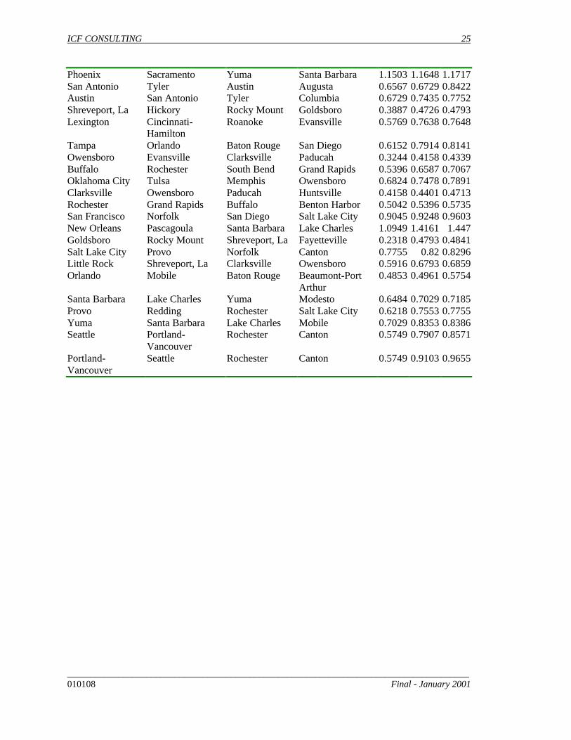
Results of the application of the homology mapping technique using the full set of vectorcomponents (to identify “prototypical” urban areas for photochemical modeling) are presented inTable 4-1. For each urban area, the three best matches are given. The Euclidean distanceassociated with each match is also provided. While this number has little or no physicalmeaning, the relative value can be used to indicate and contrast the relative fidelity of eachmatch. Note that the results are not listed alphabetically but instead have been ordered accordingto 8-hour ozone design value. In recommending areas for photochemical modeling, we attemptto include not only those areas that are good surrogates for as many other areas a possible, butalso areas represent the range of severity that characterizes ozone problems within the U.S.Specific consideration was also given to representing different regions of the country.

The ozone homologues presented in Table 3-1 may provide the basis for mapping future HIRIphotochemical modeling results (in terms of the change in ozone concentration due toimplementing HIRI measures). They also provide the basis for recommending urban areas formodeling (to provide the best basis for future use of homology mapping to extend the utility ofthe modeling results).

The three set of recommendations (corresponding to different numbers and geographicalgroupings of urban areas) as well as the stepwise procedure that was followed to arrive at therecommendations is presented in the remainder of this section.

DISCUSSION OF METHODOLOGY

We first identified (similar to for the meteorological modeling application) those areas that mostfrequently were among the best three matches for the greatest number of other areas. We thenlooked at different ranges of 8-hour ozone design value (including less than 85 ppb, 85 to lessthan 90 ppb, 90 to less than 95 ppb, etc.) and identified the same for each of these categories.We discounted those areas that had a large number of matches but for which the majority ofthese were small urban areas that were similar and nearby to one another. One such example isEvansville, IL; Owensville, KY; and Paducah, KY. These areas are very similar and very closeand are good surrogates for one another. However, they were not good general surrogates formany other areas. Similar examples occurred for smaller cities in North Carolina, Pennsylvania,and Ohio.

We also attempted to ensure that many of the larger urban areas were represented – eitherdirectly or by reasonable surrogates. This was somewhat subjective both in terms of identifyingthe key/larger urban areas as well as the degree to which a good match was found. Those areasthat were just not accommodated by the frequent match surrogates were added to the list and thusdirectly represented.

ICF CONSULTING 21

______________________________________________________________________________________010108 Final - January 2001

Two of our largest cities deserve special mention. No good match was found for either LosAngeles or New York. Since Los Angeles has been the subject of much study with respect urbanheat island mitigation, we have opted to not include it as part of our recommendations. It isimportant to note, however, that our results indicate that modeling results for Los Angeles shouldnot be used to quantify or draw conclusions about the effects of HIRI measures in other urbanareas. This is an important finding – given the amount of information that has been generated forLos Angeles. There were also no good matches found for New York – again a very unique cityin many respects. However, as discussed later, New York would likely be included in amodeling domain that includes other important surrogate cities and thus could be modeleddirectly.

Finally, from a practical perspective (given expected cost and schedule considerations) weattempted to limit our recommendations to ten different areas or modeling domains. By takingadvantage of geographical proximity of some areas to one another, we also attempted tomaximize the number of “best match” urban areas within these ten areas.

RECOMMENDATIONS

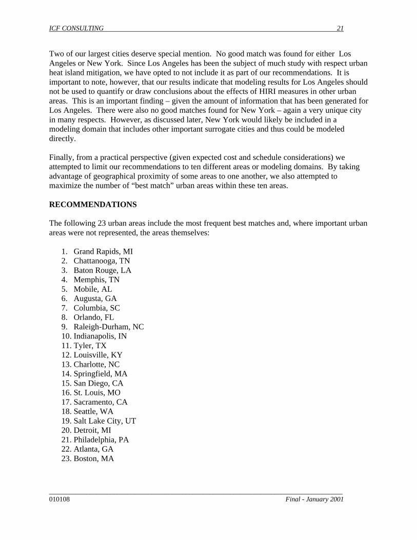
The following 23 urban areas include the most frequent best matches and, where important urbanareas were not represented, the areas themselves:

1. Grand Rapids, MI2. Chattanooga, TN3. Baton Rouge, LA4. Memphis, TN5. Mobile, AL6. Augusta, GA7. Columbia, SC8. Orlando, FL9. Raleigh-Durham, NC10. Indianapolis, IN11. Tyler, TX12. Louisville, KY13. Charlotte, NC14. Springfield, MA15. San Diego, CA16. St. Louis, MO17. Sacramento, CA18. Seattle, WA19. Salt Lake City, UT20. Detroit, MI21. Philadelphia, PA22. Atlanta, GA23. Boston, MA

22 ICF CONSULTING

______________________________________________________________________________________0101008 Final – January 2001

Based on the homology mapping results, these 23 areas could be used to represent a total of 74of the 106 urban areas considered in this analysis – using any of the three best matches andwithout considering the fidelity of the match. Using only the best match, 51 urban areas couldbe represented.

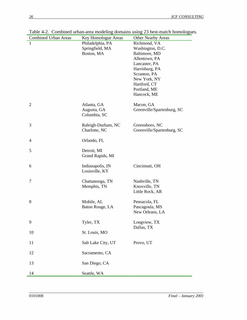
Many of these areas are near enough to one another that they could be placed within a singleregional-/urban-scale modeling domain. In defining these domains, other urban areas may alsobe included just based on proximity. For the list of cites above, possible domain groupings aregiven in Table 4-2. In addition to the key areas, other nearby areas that would also likely fallwithin a domain are listed. Please note that some of these domains (e.g., 2 and 3) may overlap.Similarly, depending upon the size of the modeling domain some of the additional areas may betoo far away to be treated with sufficient detail (i.e., to be located within the high-resolutionportion of the modeling domain).

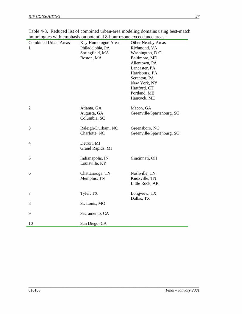
Finally, this list is shortened in Table 4-3 to ten areas comprising modeling domains. To reducethe number of domains, areas with low 8-hour design values (less than 85 were omitted). Inaddition, areas that provide the least amount of benefit (matches) for homology mapping weregiven lower priority and some were omitted. These domains include 36 urban areas from ouroriginal list (refer to Table 2-1). Based on the homology mapping results, these 36 urban areascould be used to represent a total of 69 of the 106 urban areas considered in this analysis – usingany of the three best matches and without considering the fidelity of the match. Using only thebest match, 40 urban areas could be represented. Thus, while we increase the number of areathat are directly represented by adding nearby areas, the overall representation of the cities is lessthan with the 23 best-match urban areas.

Each modeling domain would consist of a one or more coarse-resolution grids to capture theregional-scale effects on meteorology and pollutant transport and one or more high-resolutionnested grids (with approximately 4 km horizontal resolution) to enable simulation of the urban-scale effects. For combined areas that include cities that are some distance apart (e.g., GrandRapids and Detroit, MI or Tyler/Longview and Dallas, TX) multiple high resolution grids maybe used. Some recent model applications (e.g., the Gulf Coast Ozone Study), however, haveused extended high resolution grids.

As a final note on the use of homology mapping results, once the modeling domains and citiesare selected the homology mapping algorithm should be rerun using only modeled cites aspossible homologues for the not-modeled cities. Other suitable matches or mappings may exist –all results should be used with care and the fidelity of the match should be examined.

ICF CONSULTING 23

______________________________________________________________________________________010108 Final - January 2001

TABLE 4-1. Homology mapping results for photochemical modeling. ED is Euclideandistance.City Best Match 2nd Best 3rd Best 1st ED 2nd ED 3rd EDLos Angeles San Joaquin Houston. Atlanta 2.0558 2.6173 2.8421Atlanta Houston. Dallas Sacramento 0.7597 0.8723 1.0251Houston. Atlanta San Diego Sacramento 0.7597 0.8852 1.0367San Joaquin Phoenix Dallas Sacramento 1.5525 1.6835 1.7303Philadelphia Washington DC Baltimore Hartford 0.7366 0.7903 1.1089Baltimore Washington DC Allentown Philadelphia 0.4356 0.7851 0.7903New York Chicago Philadelphia Boston 1.8871 2.1494 2.4033Ventura Norfolk San Diego Modesto 0.6701 0.6873 0.76Washington DC Baltimore Philadelphia Hartford 0.4356 0.7366 0.912Knoxville Greenville Chattanooga Johnson City 0.5087 0.5234 0.6024Macon Raleigh-Durham Asheville Huntington-

Ashland0.5109 0.5792 0.6628

Charlotte Indianapolis Greenville Raleigh-Durham 0.5851 0.5874 0.5892Hartford Boston Springfield Baltimore 0.795 0.8111 0.8663Nashville Chattanooga Memphis Knoxville 0.5785 0.6421 0.669Sacramento Modesto San Diego Norfolk 0.6254 0.722 0.7532Raleigh-Durham Macon Huntington-

AshlandLongview 0.5109 0.5465 0.5591

Pittsburgh Scranton Charlotte Harrisburg 0.5279 0.7303 0.754Dallas St. Louis Charlotte Memphis 0.7107 0.8029 0.8613Lancaster Allentown York Reading 0.2788 0.3063 0.3265Longview Birmingham Augusta Shreveport, La 0.5321 0.5328 0.5346Allentown Lancaster Reading York 0.2788 0.315 0.4177Springfield Richmond Reading Canton 0.6482 0.6938 0.6954San Diego Norfolk Ventura Sacramento 0.6423 0.6873 0.722Cleveland Erie Buffalo Benton Harbor 0.7309 0.7983 0.8271Richmond Fayetteville Rocky Mount Raleigh-Durham 0.4622 0.5367 0.6192Greensboro Louisville Tulsa Cincinnati-

Hamilton1.0626 1.0703 1.0921

Scranton Pittsburgh Johnstown Parkersburg 0.5279 0.5348 0.5606Indianapolis Youngstown Columbus Charlotte 0.516 0.5396 0.5851Birmingham Longview Tyler Augusta 0.5321 0.6717 0.7023Milwaukee Cleveland Louisville Salt Lake City 0.9846 1.0726 1.0765Columbus Dayton Youngstown Grand Rapids 0.3095 0.4184 0.484Harrisburg Altoona Johnstown York 0.4319 0.4771 0.5038Green Bay Sheboygan Grand Rapids Benton Harbor 0.2441 0.3012 0.4486Louisville Evansville Cincinnati-

HamiltonIndianapolis 0.5144 0.5221 0.6675

Benton Harbor Erie Green Bay Sheboygan 0.3708 0.4486 0.4697Youngstown Columbus Indianapolis Lima 0.4184 0.516 0.5397Reading Allentown Lancaster York 0.315 0.3265 0.3397Huntington-Ashland

Charleston Johnson City Parkersburg 0.284 0.3593 0.3631

Greenville Roanoke Johnson City Knoxville 0.4348 0.5071 0.5087Cincinnati-Hamilton

Louisville Lexington Dayton 0.5221 0.5769 0.6027

Redding Indianapolis Provo Youngstown 0.601 0.6218 0.6458

24 ICF CONSULTING

______________________________________________________________________________________0101008 Final – January 2001

St. Louis Kansas City Dallas Indianapolis 0.6688 0.7107 0.7136Detroit Buffalo Pittsburgh Rochester 0.7799 0.9108 0.9411Boston Hartford Washington DC San Francisco 0.795 1.0746 1.1051Altoona Harrisburg Reading Johnstown 0.4319 0.5662 0.6715Modesto Sacramento Canton Santa Barbara 0.6254 0.7077 0.7185Paducah Memphis Evansville Owensboro 0.4171 0.4248 0.4339Memphis Paducah Evansville Owensboro 0.4171 0.4597 0.5072Norfolk San Diego Ventura Fayetteville 0.6423 0.6701 0.7035Grand Rapids Green Bay Sheboygan South Bend 0.3012 0.3429 0.4327Chattanooga Johnson City Huntington-

AshlandCharleston 0.3501 0.4485 0.4651

Dayton Columbus South Bend Grand Rapids 0.3095 0.5162 0.5519Asheville Hickory Shreveport, La Memphis 0.4068 0.5134 0.5509Evansville Owensboro Paducah Memphis 0.3244 0.4248 0.4597York Lancaster Reading Allentown 0.3063 0.3397 0.4177Johnstown Parkersburg Fort Wayne York 0.3711 0.4605 0.4643Erie Benton Harbor Rochester Green Bay 0.3708 0.6296 0.7199Chicago Detroit San Francisco Washington DC 1.0375 1.1419 1.1664Pascagoula New Orleans Lake Charles Santa Barbara 1.0949 1.1292 1.1435Sheboygan Green Bay Grand Rapids Benton Harbor 0.2441 0.3429 0.4697Augusta Tyler Rocky Mount Shreveport, La 0.4963 0.5017 0.5319Columbia Fayetteville Rocky Mount Augusta 0.4753 0.5219 0.5528Portland Springfield Hancock Canton 1.016 1.1203 1.2174Baton Rouge Beaumont-Port

ArthurMobile Lake Charles 0.4345 0.4428 0.4429

Fayetteville Rocky Mount Richmond Columbia 0.4076 0.4622 0.4753Parkersburg Charleston Huntington-

AshlandJohnstown 0.335 0.3631 0.3711

Johnson City Chattanooga Huntington-Ashland

Charleston 0.3501 0.3593 0.3684

Pensacola Beaumont-PortArthur

Baton Rouge Mobile 0.3141 0.4944 0.5072

South Bend Grand Rapids Sheboygan Dayton 0.4327 0.4909 0.5162Tyler Augusta Evansville Shreveport, La 0.4963 0.5756 0.5959Kansas City St. Louis Clarksville Chattanooga 0.6688 0.8686 0.874Canton York Fayetteville Rocky Mount 0.6241 0.6371 0.6432Charleston Huntington-

AshlandParkersburg Johnson City 0.284 0.335 0.3684

Roanoke Greenville Charleston Parkersburg 0.4348 0.4642 0.4905Huntsville Clarksville Johnson City Paducah 0.4713 0.4777 0.5836Hickory Shreveport, La Asheville Rocky Mount 0.3887 0.4068 0.4495Rocky Mount Goldsboro Fayetteville Hickory 0.2318 0.4076 0.4495Hancock Springfield Hickory Asheville 0.9963 1.0317 1.0466Beaumont-PortArthur

Pensacola Baton Rouge Goldsboro 0.3141 0.4345 0.5326

Fort Wayne Lima Johnstown Grand Rapids 0.3542 0.4605 0.4899Mobile Baton Rouge Orlando Pensacola 0.4428 0.4853 0.5072Lima Fort Wayne Youngstown Grand Rapids 0.3542 0.5397 0.5542Lake Charles Baton Rouge Mobile Orlando 0.4429 0.5714 0.6252Tulsa Oklahoma City Lexington Louisville 0.6824 0.8922 0.9353

ICF CONSULTING 25

______________________________________________________________________________________010108 Final - January 2001

Phoenix Sacramento Yuma Santa Barbara 1.1503 1.1648 1.1717San Antonio Tyler Austin Augusta 0.6567 0.6729 0.8422Austin San Antonio Tyler Columbia 0.6729 0.7435 0.7752Shreveport, La Hickory Rocky Mount Goldsboro 0.3887 0.4726 0.4793Lexington Cincinnati-

HamiltonRoanoke Evansville 0.5769 0.7638 0.7648

Tampa Orlando Baton Rouge San Diego 0.6152 0.7914 0.8141Owensboro Evansville Clarksville Paducah 0.3244 0.4158 0.4339Buffalo Rochester South Bend Grand Rapids 0.5396 0.6587 0.7067Oklahoma City Tulsa Memphis Owensboro 0.6824 0.7478 0.7891Clarksville Owensboro Paducah Huntsville 0.4158 0.4401 0.4713Rochester Grand Rapids Buffalo Benton Harbor 0.5042 0.5396 0.5735San Francisco Norfolk San Diego Salt Lake City 0.9045 0.9248 0.9603New Orleans Pascagoula Santa Barbara Lake Charles 1.0949 1.4161 1.447Goldsboro Rocky Mount Shreveport, La Fayetteville 0.2318 0.4793 0.4841Salt Lake City Provo Norfolk Canton 0.7755 0.82 0.8296Little Rock Shreveport, La Clarksville Owensboro 0.5916 0.6793 0.6859Orlando Mobile Baton Rouge Beaumont-Port

Arthur0.4853 0.4961 0.5754

Santa Barbara Lake Charles Yuma Modesto 0.6484 0.7029 0.7185Provo Redding Rochester Salt Lake City 0.6218 0.7553 0.7755Yuma Santa Barbara Lake Charles Mobile 0.7029 0.8353 0.8386Seattle Portland-

VancouverRochester Canton 0.5749 0.7907 0.8571

Portland-Vancouver

Seattle Rochester Canton 0.5749 0.9103 0.9655

26 ICF CONSULTING

______________________________________________________________________________________0101008 Final – January 2001

Table 4-2. Combined urban-area modeling domains using 23 best-match homologues.Combined Urban Areas Key Homologue Areas Other Nearby Areas1 Philadelphia, PA Richmond, VA

Springfield, MA Washington, D.C.Boston, MA Baltimore, MD

Allentown, PALancaster, PAHarrisburg, PAScranton, PANew York, NYHartford, CTPortland, MEHancock, ME

2 Atlanta, GA Macon, GAAugusta, GA Greenville/Spartenburg, SCColumbia, SC

3 Raleigh-Durham, NC Greensboro, NCCharlotte, NC Greenville/Spartenburg, SC

4 Orlando, FL

5 Detroit, MIGrand Rapids, MI

6 Indianapolis, IN Cincinnati, OHLouisville, KY

7 Chattanooga, TN Nashville, TNMemphis, TN Knoxville, TN

Little Rock, AR

8 Mobile, AL Pensacola, FLBaton Rouge, LA Pascagoula, MS

New Orleans, LA

9 Tyler, TX Longview, TXDallas, TX

10 St. Louis, MO

11 Salt Lake City, UT Provo, UT

12 Sacramento, CA

13 San Diego, CA

14 Seattle, WA

ICF CONSULTING 27

______________________________________________________________________________________010108 Final - January 2001

Table 4-3. Reduced list of combined urban-area modeling domains using best-matchhomologues with emphasis on potential 8-hour ozone exceedance areas.Combined Urban Areas Key Homologue Areas Other Nearby Areas1 Philadelphia, PA Richmond, VA

Springfield, MA Washington, D.C.Boston, MA Baltimore, MD

Allentown, PALancaster, PAHarrisburg, PAScranton, PANew York, NYHartford, CTPortland, MEHancock, ME

2 Atlanta, GA Macon, GAAugusta, GA Greenville/Spartenburg, SCColumbia, SC

3 Raleigh-Durham, NC Greensboro, NCCharlotte, NC Greenville/Spartenburg, SC

4 Detroit, MIGrand Rapids, MI

5 Indianapolis, IN Cincinnati, OHLouisville, KY

6 Chattanooga, TN Nashville, TNMemphis, TN Knoxville, TN

Little Rock, AR

7 Tyler, TX Longview, TXDallas, TX

8 St. Louis, MO

9 Sacramento, CA

10 San Diego, CA

28 ICF CONSULTING

______________________________________________________________________________________0101008 Final – January 2001

References

Iwamiya, R. K. and S. G. Douglas. 1999. “Use of a Homology Mapping Technique to EstimateOzone and Particulate Matter Concentrations for Unmonitored Areas”. TechnicalMemorandum to James B. DeMocker dated 6 April 1999. Systems ApplicationsInternational, Inc. San Rafael, California.

Oke, T. R. 1978. Boundary layer climates. Methuen and Co., New York, New York.