icfl kw - dtic
TRANSCRIPT

IcFL COP4KwENVIRONMENTAL IMPACT
RESEARCH PROGRAM
4 0 *
US Ary0 .o CONTRACT REPORT EL-89-3IF fEgpter
RESERVOIR BANK EROSION AND CULTURALI RESOURCES: EXPERIMENTS IN MAPPING AN4DPREDICTING THE EROSION OF ARCHEOLOGICAL
SEDIMENTS AT RESERVOIRS ALONG THEMIDDLE MISSOURI RIVER WITH SEQUENTIAL-
HISTORICAL AERIAL PHOTOGRAPHSby
Jam( s 1. Ebert, Eileen L. Camilli, LuAnn Wandsnider
Ebert and Associates
Albuquerque, New Mexico 87107
DTIC-IN X- E ~ECTE 1M11
o 6SEP 131989 / Y
August 1989Final Report
- -- 4Approved For Public Riflease: Distribution lnlmte(
Prepared for DEPARTMENT OF THE ARMYUS Army Corps of EngineersWashington, DC 20314-1000
ndflr Contract No. DACW39-86-C-0071-VI EIRP Work Unit 32357Monitored by Environmental LaboratoryUS Army Engineer Waterways Exp,)riment Staion
3919 Halls Ferry Road, Vicksburg, MIssissippi 3918k-61n
8913 09

Unrla~gifi edSECURITY CLASSIF1CATION OF T IS PAGE
Form AoprOveisREPORT DOCUMENTATION PAGE 0M44lVo 0'i4 O188
E'D Oaf@ Jun30 1986
la REPORT SECURITY CLASSIFICATION lb RESTRICTIVE MARKINGS
Unclassified
2a SECURITY CLASSIFICATION AUTHORITY 3 DiSTRIBUTION I AVAILABILITY OF REPORTApproved for public release;
2b DECLASSIFICATION IDOWNGRADING SCHEDULE distribution unlimited.
4 PERFORMING ORGANIZATION REPORT NUMBER(S) S MONITORING ORGANIZATION REPORT NUMBERIS)
Contract Report EL-89-3
6a NAME OF PERFORMING ORGANIZATION 6b OFFICE SYMBOL 7a NAME OF MONITORING ORGANIZATION
Ebert and Associate (if applicable) USAEWES
b n aEnvironmental Laboratory
6c. ADDRESS (City, State. and ZIPCoide) 7b ADDRESS (City. State. and ZIP Code)
Albuquerque, NM 87107 3909 Halls Ferry Road
Vicksburg, MS 39180-6199
Ba. NAME OF FUNDING i SPONSORING 8b OFFICE SYMBOL 9 PROCUREMENT INSTRUMENT IDENTIFICATION NUMBERORGANIZATION (If applicable)
US Army Corps of Engineers Contract No. DACW39-86-C-0071
8c. ADDRESS (City, State, and ZiP Code) 10 SOURCE OF FUNDING NUMBERS
PROGRAM PROJECT TASK WORK UNITE EMENT .:O Nn NO ACCESSCON Nnr
Washington, DC 20314-1000 1EIRP 32357
11. TITLE (include Security Classification) Reservoir Baik Erosion and Cultural Resources: Experiments inMapping and Predicting the Erosion of Archeological Sediments at Reservoirs Along the Middle
Missouri River with Sequential Historial Aerial Photographs
12 PERSONAL AUTHOR(S)Ebert, James I., Camilli, Eileen L., Wandsnider, LuAnn
13a TYPE OF REPORT i13b TIME COVERED 14 DATE OF REPORT (Year. Month. Day) 15 PAGE COUNTFinal reportI FROM__ TO August 1989 130
16 SUPPLEMENTARY NOTATION
See reverse.
17 COSATI CODES 18 SUBJECT TERMS (Continue on reverse if necessary and identify by block number)
'ELD GROUP SUB-GROUP Cultural resource protection Remote sensingMiddle Missouri River Reerv'oir shore!'-e
erosion
19 ABSTRACT (Continue on reverse if necessary and identify by block number)
This report reviews remote sensing capabilities for assessing archeological siteerosion using sequential, historical aerial photographs. The utility of photointerpreta-tion for measurement of bank erosion is explored to empirically document impacts tothreatened reservoir-side archeological sites and to model factors affecting differentialrates of erosion between and within such sites., The processes of bank and beach erosionare long term in nature, and sequential, historical aerial photographs offer one of thebest time-series data sources for studying reservoir bank erosion.
20 DISTRIBUTION / AVAILABILITY OF ABSTRACT I11 ABSTRACT SECURITY CLASS,FiCATION(2 UNCLASSIFIED/UNLIMITED I SAME AS RPT o DTC uSERS Unclassified
22a NAME OF RESPONSIBLE NDIVIDUAL ;2b TELEPHONE (include rea, ode) 22c OFFICE SVABOL
DD FORM 1473. 84 MAR 13 APR ecd on 'ay be uSeD unt I enausteo iE_. -Y (_ASSIICA' ON 01 '-S YAGEAll other eolton$ are oosorete Unclassified

Unclassi fipdSECURITY CLASSIFICATION OF' TMS PAGE
16. SUPPLEMENTARY NOTATION (Continued).
Available from National Technical Information Service, 5285 Port Royal Road, Springfield,VA 22161. Appendixes A and B are not reproduced herein but are available from the US ArmyEngineer Waterways Experiment Station.
SAcces on For
NTISCRDTIC TAB fJtj-anno,-.:., d C3
By
DA, 'bulturI
Avjti.jtl;ty Codes
.' , ",.'4( .
'Urc I i f iedSECURITY CLASSIFICATION OF TMIS P&GE

SUMMARY
In this research, remote sensing capabilities for assessing archeologi-
cal site erosion rate have been evaluated using sequential, historical aerial
photographs. Specifically, the utility of photointerpretation for measurement
of bank erosion using sequential, historical aerial photographs was explored
to empirically document bank erosion threatening reservoir-side archeological
sites and to model factors affecting differential rates of erosion between and
within such sites. Efforts directed toward developing a definitive and
comprehensive model of bank erosion by previous researchers have been based
upon on-the-ground measurements of bank recession. The variable results of
this research are at least partially due to the long-term nature of the
process of bank and beach erosion that cannot be monitored with sufficient
time depth by contemporary measurements. In contrast, aerial photographs
offer one of the best time-series data sources available for studying bank
erosion.
Analysis of the phenomenon of bank and site erosion has been undertaken
at several different scales: (a) the site, as more or less arbitrarily
defined by the extent of cultural features like housepits or palisade ditches;
(b) bank erosion and variability in that erosion with site areas defined as
being 2 km along active banks centered upon the site itself; and (c) bank
erosion, and its predictability, from the perspective of the overall Middle
Missouri River system.
Twelve major archeological sites situated on Corps of Engineers reser-
voirs in North Dakota, South Dakota, and Nebraska and chosen for study are a
small sample of archeological sites currently endangered by bank erosion. The
situations in which these sites are found, including the specific mechanisms
and determinants of bank erosion there, may not be representative of all bank
erosion situations on the reservoirs studied. Therefore, these sites were
believed to be representative, to some extent, of erosionally endangered
cultural resources and their situations on Middle Missouri River reservoirs.
Aerial photographs obtained from a number of government repositories
include those from the National Archives dating to the late 1930's that show
baseline, --nreqervoir erosion prior to the next series generally available
from the late 1940's to mid-1950's. Contact prints spanning the year 1949
through the present with large-scale aerial photographs ddting fror.. the early

1970's to the present were provided by the US Army Engineer District, Omaha.
Stereo photointerpretation focused on criteria best distinguishing an ero-
sional bank from a beach or waterline.
At the largest and most specific spatial scale, an electronic
enlargement/enhancement process was developed to examine bank erosion of the
immediate site area. Site area, defined on the basis of photointerpretable
indications of cultural features on the ground, was mapped and measured
digitally for successive aerial photographs. Change in site area through time
is linear, although the slope of this relationship differs among the three
sites examined. Regression analysis yielded site-area decay curves with
extinction dates predicted through the use of regression equations for three
example sites. The fact that a linear regression model fits the decay curveq
suggests that erosion rates are relatively constant through time. While a
sigmoidal model may describe bank erosion through time, the photograph dates
available document only the middle, near-linear part of the model.
At a smaller, more general scale, measurement of bank erosion focuses on
a 2-km segment of shoreline centered on sites considered. Using 1:10,000-
scale base maps of a 2-km by 2-km quadrat centered on each site, the histori-
cal sequence of photographs of each site were inspected for site specific
manifestation of beach, bank, and waterline and the positions of control
points on both the photos and base map. Transects placed at 100-m intervals
along the waterline, oriented perpendicular to the gradient or slope just
inland from the waterline, serve as objectively determined points along which
bank movement could be measured on successive photos. Using digital calipers,
the amount of displacement between the baseline (earliest) location of the
bank and the position of the bank interpreted from each stereo pair at each of
21 transects was measured. Calculating the distance between each successive
shoreline and dividing these data by the time elapsed between each photo-
graphic overflight date allows the derivation of a rate in metres per year of
recession between consecutive overflight dates. To facilitate the identifica-
tion of major factors influencing bank erosion, independent variables measured
included gradient of the land at the intersection of the transect with the
baseline shoreline, presence or absence of beach, aspect of the bank or shore,
fetch, pool level fluctuation, and soils properties.
The mean bank recession rate at individual sites, derived by averaging
measurement over all 21 transects, indicates an erosion rate of about 2.5 m or
2

8 ft per year with most sites ranging between 1.8 and 3.08 m per year. These
rates are consistent with and in some cases higher than previously reported
erosion rates based on aerial photogrammetry.
Results of regression analyses show that these bank recession rates are
to some extent at least predictable through reference to physically measur-
able, independent variables. Regression analyses designed to model rates
between measurement dates using temporal pool level data did not prove to
explain a very large proportion of variability in rates. It is possible that
the low values derived from the use of pool management data are due to the
fact that variations between measurement dates may be caused by the combined
effects of unique, high energy events between dates.
Regression analyses, modeling recession rate with nontemporal data,
suggest important differences between reservoirs. While combined site (12
study sites) predictions using nontcmporal data had low regression values,
using only aspect and fetch data did allow the explanation of between 17 and
40 percent of the spatial variability in transects in all sites within single
reservoirs. Parameter estimates calculated for regression equations within
specific reservoirs indicate that aspect is probably the most constant
estimator--that is, it has similar effects at all reservoirs. The effects of
the fetch variables differ more among reservoirs, indicating that there may be
important differences in the shapes of shorelines rather than simply the
directions they face that may be influencing bank erosion.
Projection of bank recession rates indicates, in some cases, that major
archeological sites on Middle Missouri Reservoirs will be entirely destroyed
within the next 15 to 30 years. These results indicate that archeologically
relevant bank erosion can be measured using sequential aerial photographs.
Although mean bank erosion rates at Middle Missouri River study sites are high
enough to be of immediate concern to archeologists, it is also apparent that
bank erosion rates are, at the same time, extremely variable even within
sites. This variability is in large part the result of natural factors and
may, therefore, be predictable and, thus, a realistic basis for prioritizing
cultural resource concerns.
Finally, photointerpretation noted unrecorded features and sites, in
fact continuous sites in some cases, along the bank within and beyond the 2-km
segments inspected. Thece findings underscore the value of cumulative photo-
interpretation of a series of aerial photographs of different dates and
3

types, and also suggest that in many places along the Missouri River it is not
sites per se which may be of archeological significance but entire stretches
of bank for which erosion potential must be predicted.
4

PREFACE
This study was conducted under Work Unit 32357 of the Environmental
Impact Research Program (EIRP). The EIRP is sponsored by Headquarters,
US Army Corps of Engineers (HQUSACE) and is assigned to the US Army Engineer
Waterways Experiment Station (WES) under the purview of the Environmental
Laboratory (EL). Technical monitors were Dr. John Bushman, Mr. David P.
Buelow, and Mr. Dave Mathis of HQUSACE. Dr. Roger T. Saucier, EL, WES, was
the EIRP Program Manager.
The study was performed by Ebert and Associates, Albuquerque, NM, under
Contract No. DACW39-86-C-0071. Dr. James I. Ebert served as principal inves-
tigator. The report was prepared by Dr. Ebert, Dr. Eileen L. Camilli, and
Ms. LuAnn Wandsnider and was edited by Mrs. Gilda Miller, WES, Information
Technology Laboratory, Information Products Division.
Technical reviewers of the report included the following Corps of
Engineers personnel: Dr. F. Douglas Shields, Ms. Anne MacDonald,
Mr. Robert J. Larson, and Dr. James J. Hester, all of WES, EL; Dr. Lawrence W.
Gatto, Cold Regions Research and Engineering Laboratory; Ms. Ellen Cummings,
Missouri River Division; and Messrs. Richard Berg and Edward Brodnicki,
US Army Engineer District, Omaha.
The study was conducted under the direct supervision of Dr. Shields and
under the technical editorial supervision of Dr. Hester, who was serving at
WES under an Intergovernmental Personnel Act agreement with the University of
Colorado during the time of the study. The supervisory work was performed in
the Water Resources Engineering Group (WREG), Environmental Engineering Divi-
sion (EED), EL, WES. Dr. Paul R. Schroeder, acting, and Dr. John J. Ingram
supervised the work as Chiefs of WREG; under the general supervision of
Dr. Raymond L. Montgomery, Chief, EED, and Dr. John Harrison, Chief, EL.
Acting Commander and Director of WES during preparation of the report
was LTC Jack R. Stephens, EN. Technical Director was Dr. Robert W. Whalin.
This report should be cited as follows:
Ebert, James I., Camilli, Eileen L., and Wandsnider, LuAnn. 1989."Reservoir Bank Erosion and Cultural Resources: Experiments in Mappingand Predicting the Erosion of Archeological Sediments at ReservoirsAlong the Middle Missouri River With Sequential Historical AerialPhotographs," Contract Report EL-89-3, US Army Engineer WaterwaysExperiment Station, Vicksburg, MS.
5

CONTENTS
Page
SUMMARY ..................................................................... 1
PREFACE ... .......................................................... 5
LIST OF TABLES ................... ....................................... .7
LIST OF FIGURES ............................................................ 7
CONVERSION FACTORS, NON-SI TO SI (METRIC)UNITS OF MEASUREMENT .... ........................................... 9
PART I: INTRODUCTION... ....................................... 0.... 10
Research: Orientation and Goals ............................... .. 10Setting of Missouri River Terraces ............................. .. 13Middle Missouri River Region Archeology ............................ 16
PART II: RESEARCH BACKGROUND AND METHODS ............................... 21
Aerial Archeology along the Missouri River ..................... 21Sequential Aerial Photographs for the Measurement andMapping of Bank and Shore Erosion .............................. 24
Aerial Photographs as a Data Source for the Measurement ofBank and Shore Erosion .......................................... 28
Recognition and Classification of Bank Erosion withRemote Sensing Data ........... ...... ......... ............ 35
Methods for the Measurement of Bank Erosion .................... 42Sources and Magnitude of Errors in
Measurements from Aerial Photographs ............................. 47
PART III: DATA ANALYSIS AND CONCLUSIONS ................................. 53
Bank Erosion: Causes, Processes, and Variables ................ 53Measurements, Variables, and Data Structure .................... 69Bank Recession Rates at Study Sites ......................... 71Tieldwork ........................................................... 82
Analysis of Pool Levels and Apparent Bank Recession ............. 85Aspect and Bank Recession ......................................... 89Multiple Regression Analysis ..... ............................ .93Site-Specific Measurements Using Electronic Image Analysis ..... 102Conclusions and Recommendations .................................... 113
REFERENCES ......... .................................................... 119
APPENDIX A: AERIAL PHOTOGRAPHS COVERING MIDDLEMISSOURI RIVER STUDY SITES* ................................. Al
APPENDIX B: BANK RECESSION MEASURES--SITE TABLES AND GRAPHS* ........ BI
• Appendixes A and B are not reproduced herein but are available from the US
Army Engineer Waterways Experiment Station.
6

LIST OF TABLES
No. Page
I Summary of Aerial Photographic Coverage forMiddle Missouri Sites ........................................... 27
2 Bank Recession Rates Measured from Aerial PhotographsMiddle Missouri River Reservoirs ................................ 33
3 Land Erosion Classification Levels and Taxonomies ............. 364 Photointerpretive Key Developed for the Discrimination of
Erosional Reservoir Banks along the Middle Missouri River... 38
5 Locations of the Study Sites ...................................... 436 USGS 7.5-min Topographic Quad Sheets Used
for Compiling Study Site Base Maps ................................ 44
7 Processes of Reservoir Bank Erosion andContributing Factors ............................................. 56
8 "Activating Factors" and Associated Dependent Variables
Recognized and Measured at Lake Sakakawea, ND ............... 589 Measurement, Dependent, and Independent Variables Used
in Analyses ...................................................... 7210 Overall Erosion Rates (SRATE) for Middle Missouri Sites ....... 74I1 Missouri River Sites Fieldwork, 28 Sep to 18 Oct 1987 ......... 83
12 Comparison of EDM-Measured and Aerial Photo-Measured
Bank Recession Rates ............................................. 8413 Correlations of Between-Date Measurements (RATE) and Pool
Levels for Aerial Photo Dates, by Transect .................. 8714 Between-Date Rates (RATE) for Those Sites with
General Northeast (NE) Aspects .................................. 9115 Between-Date Rates (RATE) for Those Sites with
General Southwest (SW) Aspects .................................. 9216 Results of Multiple Regression of RATE with
Fluctuation Variables ............................................ 9517 Results of Regression Analyses of RATE by Individual Sites,
Against Variables ................................................ 9618 Results of Multiple Regression Analyses of TRATE with
Normally Distributed, Nontemporal Variables ................. 9719 Results of Regression Analyses of TRATE with Normally
Distributed, Nontemporal Data ................................... 9820 Parameter Estimates for Variables in Regression Equations
Derived by Regression of TRATE with Nontemporal Variables... 10021 Extinction Dates Predicted by Regression Equations ............ 113
LIST OF FIGURES
No. Page
1 Locations of the 12 study sites in North Dakota, South
Dakota, and Nebraska ............................................ 122 Mirror stereoscope with an x-y tracking attachment ............ 45
3 Projecting interpreted bank lines to scale andrectification with a Map-O-Graph opaque projector ........... 47
4 The measurement of distances between bank lines alongtransects with digital calipers ................................. 48
7

No. Page
5 Bank erosion processes and bank characteristics contributingto erosion at northern reservoirs ............................... 57
6 Large blocks of sediment shearing from the bank at the
Jones Village Site, 39CA3 ....................................... 607 Sediments recently collapsed probably due to topple or
cantilever failure of jointed silty sediments at theJones Village Site, 39CAI ....................................... 60
8 Large numbers of huge driftwood logs pound against shores
during storms, exacerbating bank erosion .................... 619 Successive shear failures, probably caused by
freezing and thawing processes .................................. 6210 Slippage of surface soil layers during thawing causes
fenceposts in the Big Bend area to tilt in a downslope
direction ........................................................ 6211 Birds and burrowing mammals can weaken banks,
facilitating collapse, while plant roots
strengthen near-surface sediments ............................... 6312 Systematic and widespread undermining of banks during
illegal looting activities may be a major factorfacilitating bank collapse and erosion at some sites ........ 64
13 Simplified pool levels for Oahe, Fort Randall, andGavins Point reservoirs ......................................... 67
14 Lake Sakakawea pool level through time ............................ 6815 Compass rose diagram showing general a;pects
for the study sites ............................................. 9016 Site 39LM224, 26 Oct 1938 ..................................... i... . 103
17 Site 39LM224, 10 Oct 1984 ........................................ 10418 Electronic image analysis system used to edge and
contrast enhance magnified portions of aerialphotographs for site-specific mapping purposes .............. 104
19 Site 39LM224, 26 Oct 1938 ..................................... ... 105
20 Site 39LM224, I Sep 1955 ......................................... 10621 Site 39LM224, 21 Jun 1965 ........................................ 10622 Site 39LM224, 23 Jul 1969 ........................................ 107
23 Site 39LM224, 15 May 1975 ........................................ 10724 Site 39LM224, 9 Apr 1977 ......................................... 10825 Site 39LM224, 30 Oct 198i ........................................ 10826 Site 39LM224, 30 Oct 1984 ........................................ 10927 Image analysis--derived site area map of the Cable
Site, 39LM224 .................................................... 11028 Image analysis--derived site area map of the Jake
White Bull Site, 39CO6 ......................................... 11029 Image analysis--derived site area map of the
Molstad Site, 39DW234 ........................................... i1130 Measurement of areas of sites lost using a
Numonics digital planimeter .................................... I1131 Graph of extinction curves for Sites 39DW234, 39CO6,
and 39LM224 ...................................................... 112
8

CONVERSION FACTORS, NON-SI TO SI (METRIC)
UNITS OF MEASUREMENT
Non-SI units of measurement used in this report can be converted to SI
(metric) units as follows:
Multiple By To Obtain
degree (angle) 0.01745329 radians
feet 0.3048 metres
inches 2.54 centimetres
miles (US statute) 1.609347 kilometres
9

RESERVOIR BANK EROSION AND CULTURAL RESOURCES: EXPERIMENTS IN
MAPPING AND PREDICTING THE EROSION OF ARCHEOLOGICAL SEDIMENTS
AT RESERVOIRS ALONG THE MIDDLE MISSOURI RIVER WITH
SEQUENTIAL HISTORICAL AERIAL PHOTOGRAPHS
PART I: INTRODUCTION
Research: Orientation and Goals
1. This research was proposed in response to the US Army Engineer
Waterways Experiment Station (WES) Broad Agency Announcement of November 1985,
under tcpic EL-15, "Conservation of Archeological Sites," topic 7, "Remote
sensing capdbilities for assessing erosion rates, determining site extent,
location, condition, and monitoring."
2. Specifically proposed was an analysis of the utility and appropri-
ateness of using sequential, historical aerial photographs to identify the
factors contributing to the erosion or stability of a representative sample of
large, significant, and erosional1 v threatened archeological sites located on
Corps of Engineers reservoirs along the Middle Missouri River.
3. There are two major and complimentary thrusts to this research. The
first is methodological in nature, focusing on the development of efficient
and practical methods for detecting and measuring progressive erosional
changes in reservoir-related archeological sites. The second major thrust of
this research involves the identification of different types, mechanisms, and
rates of erosion and deposition at the Middle Missouri River study sites from
sequential aerial photographs. While it was envisioned that a taxonomy of
different processes contributing to site change would be compiled, along with
a photointerpretive key to their identification, it soon became apparent that,
for reasons detailed later in this report, reservoir bank erosion (and asso-
ciated aggradation in some places) is virtually the only significant process
affecting the integrity of the sites studied. A photointerpretive key was
compiled to aid in the interpretation of bank erosion from sequential aerial
photographs.
4. Deriving a definitive and comprehensive model of bank erosion pro-
cesses is beyond the scope of this research. Many previous researchers from
10

the Corps of Engineers and other agencies have directed their efforts toward
this goal. Our research, instead, is intended to supply the beginnings of a
set of methods through which archeologists, confronted with reservoir and
other water-body related threats to nrcheological sites, can utilize data
derived from sequential, historical aerial photographs to detect, measure, and
define the progression of bank recession.
5. The use of historical, sequential aerial photographs is central to
this goal. Many recent researchers interested in the processes of coastal and
reservoir bank erosion in general have based their research upon on-the-
ground, contemporary measurements of bank and beach recession, with variable
results. This may, in part, be because bank and beach erosion is a long-term
process, and contemporary measurements do not yield the time-depth necessary
to define long-term variability in the processes that cause such erosion.
Others have used historical aerial photographs, again with variable results.
Nonetheless, as discussed at length later in this report, we fePl that aerial
photographs offer one of the best data sources available for studying bank
erosion.
6. In the course of this research, we have attempted to make some
statements about the causes and predictability of erosion and erosion rates,
and how these might be correlated with measurements taker, from sequential
aerial photographs. Suggestions are made in this report about the sorts of
hydrologic, sedimentological, and other data, such as that concerning local
climatological variation, that might be needed to explain bank erosion so
detected and measured.
7. This research focuses on 12 major archeological sites along the
banks of Corps of Engineers reservoirs in North Dakota, South Dakota, and
Nebraska (Figure 1). These sites are, of course, a small sample of those
ai,1,ological sites currently endangered by bank erosion, even along reser-
voirs in those states. We do not suggest that the findings determined from
the study of these sites are representative of conditions at all res-
ervoir-side sites at these or other reservoirs. The study sites were chosen,
however, because they were believed to be to some extent representative of
archeological sites, and their situations, on these reservoirs.
8. It should also be noted that the situations in which archeological
sites are found, and therefore the mechanisms and determinants of bank erosion
in those places, may not be in general terms representative of all bank
11

32OU2
39CO6
- 39WWIS
39DW234 I
m ,39HU 173
I' 398F44
25KX57/200 39YK40
,I- MIDDLE MISSOURI RIVER
kilometere
0 so 1OO 200 a
Figure 1. Locations of the 12 study sites inNorth Dakota, South Dakota, and Nebraska
erosion situations on the reservoirs studied, or in fact in any reservoir
situation. Large archeological sites are generally thought to have beenvillages occupied either intensively with large populations or over consid-erable periods of time. It is quite likely that many careful considerations
went into locating the places in which such sites were situated, and thattheir locations are therefore somewhat unique. In addition, the intensivecultural occupation of specific areas may affect certain sedimentological
characteristics of those places, including sediment disturbance due to thedigging of house and refuse pits, and the concentration of organic materialsin sediments. These characteristics may affect the erodibility of sediments,and cause erosion in these places to be different than that of the reservoir
12

shoreline in general. While we would not automatically extend our findings to
bank erosion along reservoirs in general, we do feel that the methods of
investigation presented here represent a good starting point for investigation
of overall reservoir bank erosion.
9. Products resulting from the conduct of this research include semi-
controlled base maps representing bank position through time for each site, a
photointerpretive key for recognizing and interpreting bank positions, a
description of methods and techniques used in this study, and tabularized data
on bank position and erosion rates through time including a summary of erosion
rates at each study site. These are represented through the use of several
types of graphs. The factors which analyses suggest as being responsible for,
or at least correlated with, regional and local bank erosion on the Middle
Missouri River reservoirs are also summarized.
10. Recommendations are made concerning further research which could
reinforce, amplify, and support the results of this research. In order to
accomplish this goal, models which may aid in the explanation of the mech-
anisms and progress of bank erosion at the study sites are advanced in an
attempt to explain these processes, their progression over time, and the
variables that would have to be inspected over time in an attempt to verify
these models.
Setting of Missouri River Terraces
11. The Missouri River Basin drains an area of 1,354,564 km 2 , one-sixth
of the contiguous United States, within the Rocky Mountains, Interior Plains,
and Interior Highlands physiographic systems (Slizeski, Andersen, and Dorough
1982). Annual precipitation within its basin ranges from 25 to 127 cm per
year, depending upon whether mountain snows or seasonal rainfall supply that
water. Thus, the Missouri River was in its normal historical state subject to
devastating seasonal floods and dry periods which limited the navigation
capacity of the river system as a whole. In response to these problems, the
Corps of Engineers and uthers instituted, beginning in the 1930's, a series of
reservoir building projects to ameliorate these effects and to ensure a navi-
gable width and depth of not less than 91.4 and 2.7 m, respectively (Slizeski,
Andersen, and Dorough 1982). By 1965, the Missouri River basin contained 107
major reservoirs and 1,387 other, smaller reservoirs providing a total storage
13

capacity of over 1.38 by 1011 cu m of storage capacity (Slizeski, Andersen,
and Dorough 1982).
12. The hydrology of the Missouri River basin is a "study in hydrologi-
cal extremes" (Slizeski, Andersen, and Dorough 1982). The delay in snowmelt
in the western extremes of the basin relative to that of the plains results in
a characteristic "June rise" that both threatens flood damages downstream and
supports agriculture in semiarid western regions. When regulated, this flow
also provides a basis for year-round hydroelectric power generation as well as
allowing navigation downriver.
13. Planned as early as the 1930's, the Missouri River Bank Stabiliza-
tion and Navigation Project had as its primary objectives flood control, bank
stabilization, land reclamation, hydroelectric power generation, and develop-
ment and maintenance of a navigation channel.
14. In the ultimate furtherance of these objectives, six major dam/
reservoir systems were installed along the Missouri River between 1946 and
1963. While furthering all of the engineering contingencies envisioned by the
Corps of Engineers, Middle Missouri River reservoir construction has also
created a situation that causes occasional unique erosional threats to
archeological sites located along the terraces of the Missouri River.
15. Reservoirs are designed, and dams located, to effect optimal reser-
voir filling along river terraces--that is, reservoirs are filled to almost
the vertical extent (but not quite) circumscribed by upstream terraces. Thus,
in most places, reservoir levels lap against but somewhat below the maximum
extent of containing terraces creating a geomorphological situation in which
terrace margins are subjected to active and continuous bank erosion. Whereas
this problem might not be one of import in regions where river terraces are
comprised of highly resistant sediments, this is not the case in the Missouri
River ecosystem. The sediments against which wave and wind action encroach
along the Middle Missouri terrace system are largely composed of relatively
incompetent shales and overlying sands and silts.
16. Although the steps or terraces characterizing the physiography of
the original Missouri River valley are not everywhere present, at least five
major terraces are present in some reaches of the river in the Dakotas in
recent times. This is evidenced by accounts ranging from those of early his-
toric explorers and geologists, as well as in the course of more recent stud-
ies (Coogan 1987). These terraces have been mapped along the Missouri River
14

between Fort Thompson and Pierre, South Dakota by Coogan (1987). They have
been designated as Coogan and Irving (1959):
MT-0 The flood plain terrace of the modern river.
MT-i A terrace about 35 ft (11 m)* above themodern river at Crow Creek, south of FortThompson, exposed at Lower Brule in the1950's before the dam at Fort Thompson wasclosed.
MT-2 A terrace about 100 ft (35 m) above thepresent river level evident at Fort Thompsonat 1,420 to 1,460 ft.
MT-3 Terrace about 200 ft (65 m) above the riverevidenced on the north side of the Big BendReservoir in southern Hughes County atabout el 1,510 to 1,540 ft**
MT-4 This terrace represents the lower slopesof the Coteau du Missouri (Coogan 1987),and can be seen east of Joe Creek inHughes County, South Dakota.
17. The stratigraphy of each of these terraces consists of four major
units (Coogan 1987), deposited on the Cretaceous Pierre Shale into which the
Missouri Trench was originally cut. Overlying this bedrock unit are, in most
places, a layer of gravel, then one predominantly of sand, and lastly one of
eolian silts (loess). The latest, loess layer contains bands of humic mate-
rial representing the remnants of palaeosols, which occasionally also occur in
the sand layer. Stratigraphy is actually somewhat more complex than this
scenario in most places, the result of numerous episodes of local cutting and
filling in the Holocene.
18. Archeological remains have been found on all of these stratigraphic
layers as well as on the present ground surface. Coogan (1987) has undertaken
the task of unraveling the history of these terrace cuts to determine the
relationship between terrace fills and Pleistocene and Holocene events to pro-
vide a framework for time-stratigraphic dating of archeological sites within
the Missouri River Valley province. Working with Irving (Coogan and Irving
* A table of factors for converting non-SI units of measurement to SI
(metric) units in presented on page 9.** All elevations (el) cited herein are in feet referred to National Geodetic
Vertical Datum (NGVD) of 1929.
15
1959) and building upon the work of Clayton, Moran, and Bickley (1976), Coogan
derived a complex chronology of surfaces consisting of at least five "stable
episodes" separated by less stable, cutting, and filling episodes, spanning
the last 15,000 years. He concludes, among other things, that thin Holocene
sediments mantling the Missouri terraces and bedrock of the Missouri River
trench contain all presently known unburied and buried archeological sites in
the region, that the predominant regime during the Holocene was erosional, and
therefore that one cannot depend upon any sort of rule of thumb that buried
sites are older than unburied ones. Most known significant Missouri River
sites, from Paleoindian to historical times, lie on or within the uppermost
layers of sediment on the Missouri River terraces.
19. Investigation of bank erosion on Middle Missouri River Reservoirs,
thus, entails consideration of a number of important properties which include
such facts as:
a. When reservoirs are filled, a preformed shore and bank situa-tion exists due to the fact that terraces are already there, inplace. Terrace surfaces are very flat, while the banks againstwhich the reser-voir waters lap have a very steep gradient,approaching vertical in some cases, broken only by intermittentminor drainages which have dissected terrace margins.
b. Bank erosion is directed, in the study area, against relativelyincompetent sediments including eolian loess, silt, sand,gravels, and shales.
c. When reservoirs are filled, erosive actions are immediatelydirected toward a shoreline that has not, in the past, beensubjected to such forces. In the literature on reservoir bankerosion, it has been suggested that this occasions an initialperiod of accelerated bank erosion that should soon taper offas the bank reaches equilibrium. As will be detailed later inthis report, this is either not the case within our studyareas, or such equilibrium has apparently not been reached inthe more than 35 years since the filling of some reservoirs.
d. Due perhaps to the preferences of prehistoric peoples in thearea, many large and significant archeological sites areperched immediately on the edges of terraces, and are thus inimminent danger of impact from bank erosion.
Middle Missouri River Region Archeology
20. The Middle Missouri subarea of the Northern Plains has hosted four
major periods of prehistoric occupation. The 12 archeological sites examined
in this study represent occupations attributed to the Paleoindian Period
16

(10000 to 6000 B.C.), the Plains Archaic Period (6000 B.C. to A.D. 1), the
Plains Woodland Period (A.D. I to 900), and the Plains Village Period (A.D.
900 to 1860). While extensive discussions of human occupation of Northern
Plains can be found elsewhere (Caldwell and Henning 1978; Frison 1978; Lehmer
1971; Wedel 1961), this brief summary is intended to place the sites examined
here in perspective with respect to Middle Missouri prehistory.
Paleoindian Period(ca. 10000 to 6000 B.C.)
21. Paleoindian sites have produced the earliest documented evidence
for human occupation in the Plains with much of this evidence coming from
sites in the Northwestern Plains. Most Paleoindian manifestations identified
from the presence of finely-flaked lanceolate projectile points and extinct
Pleistocene megafauna are kill and butchering sites. These sites offer ample
evidence for exploitation of Pleistocene megafauna, principally mammoth and
bison. The Paleoindian subsistence economy may have been much more diversi-
fied, however, and may have included a wider variety of mammals and reliance
on plant resources. Faunal remains from Travis 2 (Ahler et al. 1977) in South
Dakota include the remains of bison and deer or antelope occurring in equal
frequencies. Elsewhere on the Plains, the variety of mammals represented in-
cludes deer, sheep, antelope, bison mammoth, camel, beaver, rabbit, elk,
rodents, and canids (Frison 1974, 1976; Frison et al. 1978; Frison and Bradley
1980; Wheat 1972, 1979; Wilmsen 1974). The presence of ground-stone tools at
sites such as Lindenmeler (Wilmsen 1974) also indicates reliance on plant
resources.
22. Despite the enormous effort put forth by the Federal archeological
salvage programs carried out during the 1950's and 1960's, recorded
Paleoindian and Archaic occupations in the Middle Missouri subarea are not
numerous. Lack of abundant remains attributable to this period stems chiefly
from that fact that sites representing early periods are not highly visible.
Sites either contain sparse accumulations of material or have been deeply
buried (Wood, Nickel, and Griffin 1984). Recent erosion along reservoir
shorelines has exposed previously buried archeological materials at Travis 2
(39WW15) and Walth Bay (39WW203) in South Dakota (Ahler et al. 1977; Weston,
Goulding, and Ahler 1979).
17

Plains Archaic
(ca. 6000 B.C. to A.D. 1)
23. The Plains Archaic is best known from sites in the Northwestern
Plains (Frison 1978) and least known in the Central and Northern Plains sub-
areas (Wood, Nickel, and Griffin 1984). The Archaic subsistence pattern was
one based on a wide range of resources including reliance on plant resources
(Frison 1978). Early Plains Archaic (ca. 5500 to 3000 B.C.) components are
rare on the Plains, their paucity attributed to absence of landforms and sedi-
ments of appropriate antiquity and to destruction or burial of floodplains
dating to this period (Reeves 1973). Early Plains Archaic occupations have
been recognized, however, at Travis 2 (Ahler et al. 1977) and Walth Bay (Ahler
et al. 1974) in South Dakota.
24. The variety of projectile point types attributed to the Middle
Plains Archaic (3000 to 1500 B.C.) include McKean, Hanna and Duncan types.
This period is recognized for an increased emphasis on plant foods (Frison
1978) and the appearance of roasting pits and stone circles. McKean sites
have been found in South Dakota in the Black Hills area (Sanders et al. 1987).
The Late Plains Archaic period (ca. 1500 B.C. to A.D. 1) is noted for the
distinctive corner-notched projectile points referred to as Pelican Lake.
Pelican Lake sites have been found in South Dakota around the Black Hills and
in northeastern portions of the state (Haug 1976; Nowak, Hannus, and Lueck
1982). Later large, side-notched dart-type points known as Besant are
attributed to a culture with highly organized bison hunting techniques
revolving around use of corrals (Frison 1978; Wettlaufer 1955). Besant
manifestations are included in the Late Plains Archaic by Frison (1978) and
have also been attributed to later Plains Woodland occupations.
Plains Woodland
Tradition (ca. A.D. 1 to 900)
25. Sites with Plains Woodland Tradition components are best known from
the Central Plains and the Northwestern Plains subareas from the Missouri
River eastward (Wood, Nickel, and Griffin 1984). The Plains Woodland yields
the first evidence of ceramic manufacture and domesticated plants, but perhaps
is more widely recognized as the period of mound construction on the plains.
Kansas City Hopewell or Middle Woodland sites along the Missouri River in the
eastern Central Plains include large open air habitations and campsites
located in the river bottoms (Caldwell and Henning 1978; Johnson 1976).
18

Although early evidence of cultigens is present, most Woodland occupations
represent a hunting and gathering subsistence pattern supplemented by agricul-
ture (Johnson 1976; Wedel 1961).
26. Deposits yielding Woodland components represented by thickened
cord-roughened ceramics and medium to large stemmed or corner-notched pro-
jectile points were known from early investigations of Middle Missouri sites
(Wedel 1961) and have been noted as rather common in the Middle Missouri sub-
area of the Plains (Toom and Picha 1984). Woodland sites consist of campsites
containing large quantities of bison bone, bone tools, shell, ceramic-chipped
and ground-stone tools, and Besant projectile point types, although mound
locations are more commonly known (Neuman 1975). Toom and Picha (1984)
attribute the appa-ent higher frequency of mound sites to their higher visi-
bility and to deeply buried contexts of campsites.
Plains VillageTradition (A.D. 900 to 1862)
27. The subsistence strategy during the Plains Village period was based
on horticulture practiced in bottomland and riverine settings and bison hunt-
ing. Cultigens included corn, beans, squash, and, occasionally, sunflower.
Plains Village sites consist of permanent settlements composed of earth-lodge
structures some of which are surrounded by ditch or other type of fortifica-
tion (Lehmer 1971; Wedel 1978; Wood, Nickel, and Griffin 1974). Middle
Missouri subarea villages were situated on the floodplain and on level ter-
races overlooking the extensive bottomlands of the Missouri in the vicinity of
tributary drainages. Although earth-lodge villages are a central feature of
this period, dwellings and villages appear to have been seasonally occupied.
Site types other than extensive earth-lodge villages are not as well known but
include isolated earthlodges, campsites, burials, and artifact scatters.
28. Ceramic inventory, earth-lodge shape and construction, general
artifact inventory, presence of fortifications, and geographical distribution
have been used to distinguish between the two Plains Village traditions. The
Middle Missouri Tradition was thought to have originated in the eastern wood-
lands or to have developed in place from the Plains Woodland Tradition (Lehmer
1971) and the Coalescent Tradition to have emerged from the Central Plains.
Lehmer divides the Middle Missouri Tradition into the initial (A.D. 900 to
1400), extended (A.D. 1100 to 1550) and terminal (A.D. 1550 to 1675) variants.
Subdivisions of the Coalescent Tradition are the initial (A.D. 1400 to 1550),
19
extended (A.D. 1550 to 1675), postcontact (A.D. 1675 to 1780) and disorganized
(A.D. 1780 to 1862) variants. Recent studies have called for revision of the
above taxonomy, some concluding that diffetences between variants may be more
apparent than real (Steinacher 1983).
29. The coalescence of village lifeways has been viewed as culminating
with the Arikara, Mandan, and Hidatsa village tribes. Great smallpox
epidemics in 1780 and 1781, 1801 and 1802, 1837 and 1838, and 1856 decimated
the populations of large villages along the Middle Missouri River with 30 to
98 percent mortality rates (Lehmer 1971), while measles, chickenpox, and
cholera also took their toll. The sites examined in this study were selected
by the US Army Corps of Engineers because they represent significant
archeological resources on the Middle Missouri presently threatened by bank
erosion. These sites are representative of the range of occupation periods
reviewed present in the Middle Missouri subarea. Of the Plains Village sites
examined, Molstad (39W234), Whistling Elk (39HU242), Jake White Bull (39C06),
and the Cable Site (39LM224) are presently listed in the National Register of
Historic Places. The majority of evidence for the village way of life of past
peoples on the Plains is contained in village sites such as these. The
topographic or chronologic context of other sites examined may provide unique
insights into the lifeways of early nomadic peoples as well as into the mobile
aspects of later occupations. As such, these less visible sites have been
recommended as potentially eligible for nominatioi to the National Register.
20

PART II: RESEARCH BACKGROUND AND METHODS
Aerial Archeology along the Missouri River
30. The prominent structural remains of large, often fortified villages
constructed by the prehistoric Plains Village Tradition inhabitants of the
Middle Missouri region as well as by historic Mandan, Hidatsa, and Arikara
have drawn the attention of aerial archeologists since the 1940's.
William Duncan Strong, a pioneer of Plains archeology, unsuccessfully at-
tempted to convince COL Charles Lindbergh to fly up the Missouri River to pho-
tograph earth-lodge villages shortly after the Lindberghs published their
spectacular aerial views of southwestern Pueblos in the early 1930's (Wood,
Nickel, and Griffin 1984).
31. In the late 1930's the US Department of Agriculture (USDA) began a
systematic program of vertical aerial photographic coverage of the Dakotas at
scales of approximately 1:20,000; these black-and-white aerial photographs
were first used for the systematic location and inspection of archeological
sites there by Thomas E. Huddleston, then with the US Army Engineer District,
Omaha. Beginning about 1945, Huddleston (1948) relates that his:
...attention was drawn to the fact that a number of locationsalong the upper Missouri River, which are marked 'Ancient IndianVillage' on the 1890 Corps of Engineers Maps, presented a very
singular appearance on aerial photographs...
32. Huddleston urged archeologists to use such aerial photographs to
prepare planimetric maps of the sites. He noted that the earliest available
aerial photos (from 1937 and 1938) were possibly better data sources for such
mapping than more recent coverage, because they had been taken during the
dustbowl drought when luxuriant vegetation to be found on terrace surfaces was
growing in depressions formed by earthlodges and fortification ditches, nour-
ished by organic culturally deposited materials. He provided Waldo Wedel and
Paul Cooper of the Smithsonian Institution's Missouri River Basin Surveys
(MRBS) office, initiated in 1946 in Lincoln, NE, with aerial photographs and a
list of 60 archeological sites lccated using these photographs (Wood, Nickel,
and Griffin 1984). The MRBS, under the direction of these two pioneers, con-
tinued to amass aerial photographs of their study areas and used them con-
stantly and systematically, recording possible sites on survey maps and using
21

them and subsequent aerial coverage to choose sites and plan for their
excavation.
33. Waldo Wedel flew over the Medicine Creek Reservoir in western Ne-
braska in a small aircraft to obtain the first specifically archeological aer-
ial photographs in the Plains region in the mid 1940's. Shortly thereafter,
he obtained additional oblique coverage of several major village sites, in-
cluding the Buffalo Pasture Site (39ST6) and the Sully Site (39SL4) in what
was to become the lower Oahe Reservoir area. Subsequently, Wedel and other
MRBS archeologists made hundreds of aerial overflights to photograph and docu-
ment archeological sites along the Missouri (Wood, Nickel, and Griffin 1984).
34. In the summer of 1952, the Smithsonian Institution commissioned
Ralph Soleckf to fly over and systematically photograph sites at eight planned
reservoirs in Nebraska, South Dakota, North Dakota, and Wyoming. Solecki and
his cameraman, Nathaniel L. Dewell, flew more than 8,000 km, photographing
62 archeological sites in black-and-white and color emulsions from the precar-
ious altitude of 150 to 250 m. Most of these sites are currently inundated or
significantly altered by reservoir related processes. Solecki reported on his
methods and results in two early publications (Solecki 1952, 1957).
35. A decade after Solecki's overflights, John M. Corbett, the Chief
Archeologist of the National Park Service, sought to revive aerial archeologi-
cal interests in the Middle Missouri region through the initiation of what
then seemed a novel series of experiments. These experiments, conducted by
the ITEK Corporation (ITEK 1965a, 1965b) for the National Park Service's Mid-
west Archeological Center, focused on the intensive interpretation of various
scales of black-and-white and color aerial photographs flown over two study
areas. One area measured 8 by 10 miles and was situated along the west bank
of the river near Fort George Island in Stanley County, South Dakota, and the
other area measured 6 miles in length and was located near Dores Island in
Hughes County.
36. The photographs inspected in the ITEK study included USDA vertical
black-and-white photos at an approximate 1:20,000 scale taken in 1938 and
1962, as well as 1:10,000-, 1:5,000-, and 1:3,000-scale black-and-white,
color, and color infrared photos taken specifically for the project. Hand-
held, 35-mm color photographs were also taken. These photographs were
inspected using 2x and 4x monoscopic magnifiers, and a binocular stereoscope.
37. In the 8- by 10-mile study area on the Crow Creek Indian
22

Reservation, inspection of 47 prints yielded identifications of 22 probable
sites, which were mapped on a 1:41,100-scale base map. ITEK concluded that
1:10,000-scale black-and-white and color aerial photographs yielded the best
results in their experiment, although they also remarked that the 1938 USDA
photos were excellent since they showed stressed vegetation and brought out
village sites for this reason.
38. ITEK also advanced the opinion that their experiment resulted, in
the areas studied, in a more complete and accurate survey than was previously
done by the Missouri River Basin Survey. This claim, perhaps more than any
other aspect of their work and conclusions, was to earn them and their methods
the abject spite of MRBS reviewers. In an "Analysis Memo" commenting on the
ITEK reports, addressed to Dr. Robert L. Stephenson, Director of the
Smithsonian River Basin Survey from Warren W. Caldwell, Chief of the Missouri
River Basin Project, it was contended that only 8 of ITEK's 22 sites could be
verified on the ground, that 25 additional known sites in their study area
were not seen, and that the only positives they identified were large and very
obvious. Aerial photointerpretation moneys, in Caldwell's opinion, would be
better spent on ground-based investigations.
39. A number of reasons for the hostility engendered by the ITEK report
are enumerated by Wood, Nickel, and Griffin (1984). First, ITEK erroneously
made the claim that they had "found every site which had been found by profes-
sional archeologists on the ground, (so that) field exploration which may
otherwise take months to conduct can be performed in just a few hours"
(Strandberg 1967), when in fact only about 30 percent of such sites were actu-
ally photointerpreted. Another is the rather bizarre claim by Strandberg in
the same paper that one of these sites was "discovered by photoarcheology" (it
was in fact not), and that it (39HU61, the Grannie Two Hearts Site) had been
inhabited by Norsemen. In actuality, it is a two-component site of the Ini-
tial Middle Missouri Tradition (Wood, Nickel, and Griffin 1984).
40. Some more recent aerial archeological research carried out along
the Middle Missouri River was conducted in the Big Bend Reservoir by the Divi-
sion of Archeological Research, University of Nebraska-Lincoln, employing en-
larged (1:8,100) prints of 1938-1939 USDA black-and-white aerial photographs
and two additional Corps of Engineers overflights, both at 1:24,000 scale,
from 1968 and 1974. Photographs were used as the basis of site identifica-
tion, verification, locational control, site definition and bounding, and site
23

mapping; visual inspection was supplemented by 5x, lOx, and 60x magnification,
and stereoscopic viewing. Project Director Terry L. Steinacher cites the dis-
covery of a number of sites, as well as the "misidentification" of features
that turned out to be old haystack rings and "topographic aberrations" (Wood,
Nickel, and Griffin 1984). The most immediately useful outcome of these ex-
periments was the use of the aerial photos for establishing, documenting, and
illustrating site boundaries necessary for National Register nominations.
Photos taken in early spring or late summer during dry years, it was observed,
show more cultural feature detail than others.
41. Aerial photographs, then, have provided a valuable data source for
archeologists in the Middle Missouri River region for more than 30 years. The
archeological use of aerial photographs in this area, however, has focused
almost exclusively on simply looking for evidence--largely crop marks or vege-
tative indicators--of major prehistoric and historic cultural features associ-
ated with large house pit villages and fortifications. Some researchers have
also used aerial photographs for defining site boundaries (a subject which
will be discussed elsewhere in this report), and for site mapping. This lat-
ter use, in all cases of which we are aware, constitutes sketch mapping of
visible structural cultural evidence from aerial photos.
42. The goals of this project--the interpretation and measurement of
bank through time--were somewhat at variance with such previous archeological
uses of aerial photographs along the Middle Missouri. For this reason, in
order to develop and validate appropriate methods, this study goes beyond
specifically archeological applications in the immediate study area and builds
upon methods developed across the country for using aerial photographs for the
measurement of bank and shore erosion through time.
Sequential Aerial Photographs for the Measurement andMapping of Bank and Shore Erosion
Historical aerial photographcoverage in the United States
43. Aerial photographs lend themselves to the measurement of change in
the environment and its characteristics through time for a number of reasons.
First, available aerial photographs have a considerable time-depth span in the
1'nited States. Systematic aerial photographic coverage of most of the country
was initiated in the mid-1930's by the USDA for agricultural field, soils, and
24

irrigation mapping purposes. Shortly thereafter, the US Geological Survey
(USGS) began its own systematic and repetitive mapping photography acquisition
programs. After a hiatus in aerial photo acquisition (at least in the United
States, if not in Europe and the Pacific) during World War II, the USGS re-
newed the periodic mapping coverage for the compilation of a new 7.5-min map
series. The late 1950's and 1960's saw most other Federal land-management
agencies, including the Bureau of Land Management, USDA Forest Service, Bureau
of Reclamation, and National Park Service begin their own aerial photographic
programs. Agencies involved in engineering planning, especially the Corps of
Engineers, have always used relatively large-scale controlled metric aerial
photographs taken with a calibrated camera for engineering mapping purposes,
and retake aerial photos of their project areas periodically.
44. In the early 1970's, the National Aeronautics and Space Administra-
tion (NASA) joined in the reconnaissance experimentation, and many military
and NASA high-altitude photographs were included in the USGS's national aerial
photograph and remote sensor data archive at the EROS Data Center, in Sioux
Falls, SD. The first Landsat (then ERTS) satellite was launched, and began to
supply regular, country- (and world-) wide multispectral scanner (MSS) data
with which aerial photographs could be supplemented.
45. In the late 1970's a number of government agencies initiated co-
operation in the National High Altitude Photography Program designed to pro-
vide a "next generation" of high-resolution, systematic black-and-white and
color infrared aerial photographs for the new metric-system mapping efforts,
as well as revision of land use and land cover mapping.
46. At the same time that Federal agencies and programs have been ac-
quiring aerial photographs of large areas of our country, many state and local
government offices, as well as private engineering and aerial photography
firms, have also been flying smaller areas and projects.
47. Consequently, for almost every study area chosen for any purpose in
the United States, one can be assured of finding not just one or a few, but
many, sets of high-quality aerial photographs through time. Beginning as
early as 1934 in the eastern United States, and 1936 farther west, vertical
black-and-white aerial photos at scales of between about 1:20,000 and 1:30,000
are uniformly available (except for a few states for which, unfortunately,
these older aerial negatives were destroyed as a housekeeping measure by the
National Archives). Additional coverage is available at least once in the
25

mid-to-late 1940's; by the early 1950's many overflights at a much wider range
of scales (1:5,000 through about 1:60,000) become common. In the 1970's, even
higher altitude overflights became practical, and scales reached 1:130,000 or
so. These scales are not necessarily very useful for defining and mapping the
precise locations of eroding banks, although there is much information that
they can yield, especially when subjected to image analysis (enlargement and
edge enhancement), as will be detailed later in this report.
Aerial coverage of the study area
48. Information concerning the availability of aerial photos was sought
from the USGS EROS Data Center, the USDA Soil Conservation Service (SCS), the
US Army Engineer District, Omaha, the Bureau of Reclamation, the National
Archives, and the natural resources and highway departments in Nebraska, South
Dakota, and North Dakota.
49. This search proved very successful, yielding at least 14 and in one
case as many as 28 sets of aerial photos for each study site. Dates ranged
from 1938 through 1986, and scales from 1:12,000 to 1:129,000. Black-and-
white, color, and color infrared emulsions were all available for most of the
sites. Characteristics of the aerial photos for each of the study sites are
summarized in Table 1, and individually listed in greater detail in
Appendix A.
Sequential aerialphotographs in archeology
50. The use of sequential aerial photographs and their cumulative pho-
tointerpretation, or measuring changes in and impacts to sites, by archeo-
logists in the United States has been rare. However, archeologists have used
sequential, historical aerial photographs to detect changes through time in
some southwestern Indian Pueblos (Stubbs 1950; Zubrow 1974) and metric terres-
trial photos monitoring structural sites (Ebert 1982, 1984; Lyons and Ebert
1982). Americau archeologists' uses of aerial photographs and remote sensing
have been, for the most part, one-time applications such as looking for visi-
ble evidence of undiscovered sites, mapping environmental characteristics in
the vicinity of sites, or documenting sites for cultural management purposes.
51. While the necessity of using a series of sequential aerial photo-
graphs is quite obvious in this research, to measure sequential positions of
reservoirs banks, what might be thought of as cumulative photointerpretation,
can be quite beneficial. This principle is well-known in Europe and England,
26
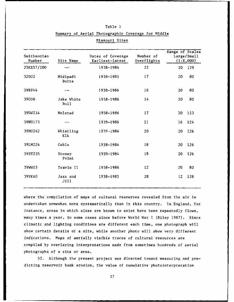
Table I
Summary of Aerial Photographic Coverage for Middle
Missouri Sites
Range of ScalesSmithsonian Dates of Coverage Number of Large/SmallNumber Site Name Earliest-latest Overflights (1:X,000)
25KX57/200 -- 1938-1984 22 20 129
32DU2 Midipadi 1938-1985 17 20 80Butte
39BF44 -- 1938-1986 16 20 80
39CO6 Jake White 1938-1986 14 20 80Bull
39DW234 Molstad 1938-1986 17 20 123
39HU173 -- 1939-1986 21 16 124
39HU242 Whistling 1939-1984 20 20 126Elk
39LM224 Cable 1938-1984 18 20 126
39ST235 Stoney 1939-1984 18 20 126Point
39WW15 Travis II 1938-1986 12 20 80
39YK40 Jazz and 1938-1985 28 12 128Jill
where the compilation of maps of cultural resources revealed from the air is
undertaken somewhat more systematically than in this country. In England, for
instance, areas in which sites are known to exist have been repeatedly flown,
many times a year, in some cases since before World War I (Riley 1987). Since
climatic and lighting conditions are different each time, one photograph will
show certain details of a site, while another photo will show very different
indications. Maps of aerially visible traces of cultural resources are
compiled by overlaying interpretations made from sometimes hundreds of aerial
photographs of a site or area.
52. Although the present project was directed toward measuring and pre-
dicting reservoir bank erosion, the value of cumulative photointerpretation
27

was apparent at a number of the study sites where the total picture of house-
pit locations, fortification ditches, and the like could be seen only whe.
features visible on a number of overflights were compiled. The cultural indi-
cations shown on the three maps compiled through electronic image analysis
means, to be described in more detail in the following paragraphs, resulted
from such cumulative mapping.
Aerial Photographs as a Data Source forMeasurement of Bank and Shore Erosion
Oceans and major lakes
53. Although archeologists, to our knowledge, have not systematically
applied sequential aerial photographs for the measurement of erosion to arche-
ological sites, a number of :'cientists have experimented with and developed
methods for measuring bank and shore erosion in general. The methods used in
this study build upon these prior efforts. Their comments about some of the
problems encountered during the course of such research, as well as their
findings, are also interesting in the light of the conclusions reached in this
study.
54. Researchers at the University of Virginia in Charlottesville em-
ployed vertical aerial mapping photographs to map beach erosion along 630 km
of the Atlantic coast between New Jersey and North Carolina (Dolan, Hayden,
and Heywood 1978; Dolan et al. 1979, 1980). These scientists note that the
use of historical aerial photographs is the most cost-effective means of de-
tecting and mapping erosion, since no other method provides the necessary
time-base for processes that take place relatively slowly. Their "Orthogonal
Grid Mapping System" (OGMS) (Dolan, Hayden, and Heywood 1978) involved the
establishment of an offshore baseline from which measurements of shoreline
position were made from aerial photographs enlarged by projection to fit a
1:5,000-scale base map. Measurements were taken at regular intervals of
100 m. Measurements from photographs from 1930, 1940, 1949, 1962, and 1970
were made of both a vegetation line demarcating the beach itself, and the
visible high-water line (rather than the visible waterline itself). Differ-
ences between these measurements were shown in graphs illustrating both mean
rate through time and their variance (one standard deviation to each side of
the mean). The prediction of future shoreline positions was approached
through the use of a linear empirical model:
28

dS = dT[(rate of change) + k(standard deviation)]
where S is the landward limit of the shoreline for a given time interval
(dT), and k is the number of standard deviations required to give a desired
probability level.
55. Mean shoreline recession rates averaged 1.5 m/yr, with high rates
of as much as 10 m/yr (Dolan et al. 1979, 1980). In estimating the level of
possible error contained in their measurements and therefore predictions,
Dolan et al. (1980) discount the significance of within-image scale variations
and radial displacement errors in aerial photographs since they are taken
along sedimentary coasts, which are of course quite level. Other errors are
due to photographic resolution, the enlargement of photographs to fit base
maps, the difficulty of precisely matching photos with the base maps, the dif-
ficulties in defining precise edges, digitizing shoreline positions, and the
idiosyncrasies of interpreters and digitizer operators. These errors result,
they say, in a "combined potential error in measurements from two photographs
at 1:5,000 scale" of 12.5 m. Since three major sources of error are summed in
this estimate (photo enlargement error, digitizing error, and interpreter
error), "each with a .5 probability" (Dolan et al. 1980), the joint probabil-
ity of this error is 0.125, which, when normally distributed about zero error
should have a standard deviation of 6.3 m. In some cases, they contend, meas-
urements are far closer than this figure, within I m of "known ground dis-
tances." In any case, Dolan et al. (1980) conclude this error amounts to
±0.32 m/yr, over a 40-year period. This conclusion puts the precision of
their OGMS methods "well within the year-to-year variance of the natural beach
system."
56. Another shoreline measurement experiment involving some of the same
researchers (Shabica et al. 1984) used the OGMS method, but was directed
toward barrier islands in the Gulf of Mexico. Interpretation instruments in-
cluded a K&E Kargl reflecting projector and a Bausch & Lomb Zoom Transfer
Scope. The measurement interval was 100 m, as before, and error and other
parameters are cited as being the same as well. As many as 10 sets of aerial
photographs spanning slightly more than 56 years were measured, and average
erosion rates ranged from 3.1 to 7.4 m/yr. Shabica et al. (1984) conclude
that today's shoreline erosion rates are closely representative of those of
29

the last 25 to 50 years and should be considered indicative of trends in the
near future.
57. Also focusing on natural (i.e. nonreservoir) shore erosion, this
time along the Ohio side of Lake Erie, Carter and Guy (1983) employed historic
maps as well as sequential aerial photographs to map shoreline recession from
1876 to 1973. Their goal was both the prediction of future shoreline changes
and the study of reasons for observed nonuniformity in erosion rates, even at
places in close proximity to one another. Shores shown on US Army Corps of
Engineer Lake Survey field maps at 1:10,000 scale were compared with those in-
terpreted from 1938 and 1973 aerial photographs at scales of 1:7,900 and
1.4,800, respectively. For comparison, the smaller-scale photos and maps were
projected to the 1:4,800 scale of the 1973 photos using a Map-O-Graph R projec-
tor. Control was accomplished through the matching of cultural and geographic
detail; the lack of many cultural control points (building, roads, etc.) be-
tween the 1976 maps and later photographs made this difficult in some cases.
58. Rather than measuring shore recession along regularly spaced tran-
sects, Carter and Guy (1983) drew the three continuous, consecutive shorelines
on base maps and then measured the alongshore length of areas of differential
recession rates between obvious break points. Their recession classes were:
very slow, <1 ft/yr; slow, 1 to 3 ft/yr; moderate, 3 to 5 ft/yr; rapid, 5 to
7 ft/yr; and very rapid, 7 to 9 ft/yr. Based primarily on the 1938-1973 aver-
age rate, a "2010 line" (Carter and Guy 1983) representing their prediction
for the shore's location in the year 2010 was also drawn. They observe that
early erosion rates were much higher prior to the building of shore protection
structures in the mid-1930's and later, and that banks rather than discrete
sandy beaches characterized the 1876 shoreline of Lake Erie.
59. A recent ocean shore measurement project undertaken at the Univers-
ity of Connecticut (Civco, Kennard, and Lefor 1986) supplements the use of
historic aerial photographs with computer assisted analysis for the identifi-
cation of salt-marsh vegetation types, changes in the area of which are the
focus of that study. Aerial photographs from 1934, 1951, 1965, 1970, and 1981
at 1:12,000 through 1:20,000 scale were interpreted, and maps of three salt
marsh areas were prepared using a Zoom Transfer Scope at 1:2,400 scale.2
Vegetation units as small as I m , according to the authors, could be mapped.
The hand-drawn vegetation maps were then converted through the use of a
drafted grid overlay into raster or picture element format; encoding maps with
30

an electronic digitizer was found to be more prone to errors than a totally
annual approach. Comparisons between areas of vegetative zones or units from
1 year to the next were then made automatically by the computer, working upon
the gridded matrix of values for each set of aerial photos.
Reservoir Bank Recession Studies
60. Perhaps the most comprehensive erosion study using aerial photo-
graphic data that is directed primarily toward reservoir bank erosion is that
carried out over the last decade by Lawrence W. Gatto and William W. Doe III,
at the US Army Corps of Engineers Cold Regions Research and Engineering Labor-
atory (CRREL). Using data from aerial photographs and other sources, Gatto
and Doe have studied reservoir (and reservoir-associated river) bank erosion
processes and trends at a large number of study sites around the country
(Gatto and Doe 1983, 1987; Gatto 1982a, 1984a, 1984b, 1988). Citing at least
34 processes which influence the type and rate of bank erosion at reservoirs,
Gatto and Doe (1983) selected 10 representative northern reservoirs (from an
initial sample of 30) for historical bank recession analyses. These analyses
were based partially on the availability of aerial photographs and the fact
that at these reservoirs bank erosion was recognized as a problem threatening
private property, recreation areas, or other site stabilization measures.
Several of their study reservoirs, including Ft. Peck, Sakakawea, and Oahe,
are on the Middle Missouri River.
61. Aerial photo coverage was selected on the basis of photo quality,
visibility of banklines and control or reference points, the availability of
stereo coverage, and time span represented. At most study sites, a 20- to 30-
year span between first and last photo dates was found. Immediately upon in-
spection of aerial coverage, it became apparent, that, at all the study sites,
bank erosion was extremely variable even within small study areas and that
"recession measurements along two or three transects may not adequately char-
acterize recession for a given bank reach" (Gatto and Doe 1983). Although
personnel from Corps offices in all regions had informally observed actual
bank erosion, these authors could find no reports, literature, or other
evidence of systematic studies or data collection on bank recession at any of
their study reservoirs.
62. Photographic control was derived by selecting stable features visi-
ble on all repetitive photos, chosen so that a line drawn between them would
be, as closely as possible, parallel to the local orientation of the bank.
31

According to Gatto and Doe (1983), transects perpendicular to the baseline
were then drawn:
... because of the geometric distortions in the photographs anddifferent photographic scales, these transects did not always passthrough the same ground features on all of the photographs for asite, so the positions of the transects were adjusted...
The intersections of the transects and the banklines were marked on the photo-
graphs while viewing stereoscopically with an Old Delft stereoscope at
4.5 power. The photograph distances from the baseline to bankline were then
measured along the transects while viewing with a 4.0-power magnifier, and
converted into equivalent ground distances using average photographic scale
for the site.
63. Calculated rates of recession varied between 0 and 39 ft/yr; bank
recession rates at Middle River sites are shown in Table 2. It is interesting
to note that these rates, up to approximately 22 m/yr, and averaging about
7 m/yr, are of the same general magnitude (if not slightly higher) as the
rates measured in the course of the present study of sites on Oahe and
Sakakawea reservoirs. In a shorter and more recent description of their
research, Gatto and Doe (1987) cite average erosion rates from the same study
in metric units (shown within brackets in Table 2). One class of parameters
Gatto and Doe address is the potential error which might result from using
aerial photographs to measure bank recession. Error causing factors they list
(Gatto and Doe 1983) include photo scale variations due to camera lens distor-
tions; aircraft altitude changes; radial, relief, and tilt distortions; lack
of useful reference or control points; obscured banklines; errors in calcu-
lating scale when using maps to determine ground distances; and human errors
when making measurements from photographs.
64. On the basis of estimates of the errors in their aerial photo-
graphic measurements, Gatto and Doe (1983, 1987) calculate a "minimum
measurable distance" (MMD) after Tanner (1978), which represents a "confidence
level for photographic measurements" (Gatto and Doe 1983). Gatto and Doe
(1983, 1987) also analyzed their measured recession figures in a number of
ways in an attempt to assess the factors responsible for erosion at their
10 study reservoirs. A series of linear regression analyses were performed to
determine whether pool levels, bank sediment textures, shoreline orientation
relative to dominant wind direction, mean annual wind speed, reservoir
32

Table 2
Bank Recession Rates Measured from Aerial Photographs, Middle
Missouri River Reservoirs (after Gatto and Doe 1983, 1987)
Study Transects RecessionReservoir Sites (Total) Years Rate
Oahe 2 11 1968-1970 68 ft/yr1970-1976 23 ft/yr
[Metric: 11.9 m/yr]
Sakakawea 3 11 1958-1966 514 ft/yr
1966-1976 19 ft/yr
[Metric: 5.2 m/yr]
Fort Peck 1 4 1950-1958 53 ft/yr
1958-1978 4 ft/yr
[Metric: 0.9 m/yr]
drainage area, surface area, mean outflow, reservoir age, or the durations of
the rainy season, the freeze-thaw season, or reservoir ice cover showed a
linear relationship with measured recession rates.
65. Unfortunately, the "...results of most of the regressions, however,
proved to be unreasonable and were not useful..." (Gatto and Doe 1983). The
only moderately high correlations with recession rates were provided by dura-2
tion of freeze-thaw and frozen-ground seasons and ice cover (r = 0.65) and
reservoir drainage area (r2 = 0.83). At the same time, it was reasoned that
other factors (wind direction, wind speed, and bank sediment characteristics)
showed no correlation whatsoever and should have been very influential. A
lack of correlation with reservoir age indicated that recession may be con-
stant over the life of a reservoir, although Gatto and Doe (1987)
...believe... that if recession continues, its rate would likelydecrease with age as an equilibrium develops between bank condi-tions and normal reservoir water level fluctuations. If there isa long term rise in the normal water level, then recession wouldprobably increase...
66. Gatto and Doe attempted to utilize aerial photographs with a con-
sideration of photographic measurement errors and stated:
33

... the data derived from aerial photographs are estimates at
best... (Gatto and Doe 1987).
and
For measuring on-going bank recession, aerial photographs do notshow the detail necessary and, if uncorrected photographs areused, contain inherent distortions which can cause large measure-ment errors... (Gatto 1984a)
They also, however, cite the possibility that average rates are not necessar-
ily actual (Gatto and Doe 1987), that correlations based on small samples may
be unreliable, and that the values used for independent variables may not be
calculated with high enough resolution to be specific to the study sites and
transects at those sites. Linear regressions, they also note, may not provide
the best models for bank recession analysis. Lumping bank recession data from
10 reservoirs across the northern portion of the country might also obscure
patterning specific to single or hydrologically and climatically related
reservoirs.
67. To collect historical bank recession data in contrast to the con-
temporary measurements made on the ground, Millsop (1985) utilizes USDA verti-
cal aerial photos taken in 1958, 1966, and 1976 at scales of 1:20,000 and
1:40,000. Millsop's (1985) annual bank recession measurements made from the
aerial photographs at Lake Sakakawea between 1966 and 1976 ranged from 1.2 to
4.3 m/yr, and averaged 2.2 m/yr. He notes that these rates also correspond
closely with rates measured at higher resolution by measuring between pins
placed on the ground. He also notes that bank recession rates for Lake
Sakakawea, measured for the same years, by Gatto and Doe (1983) were quite
different, ranging from 1.8 to 13.1 m/yr, an averaging 5.8 m/yr. This dis-
crepancy might, Millsop (1985) feels, be due to the inaccuracies of measuring
from small-scale aerial photographs; he felt that his measurements from
1:40,000-scale photos might be far less accurate than those from the
1:20,000-scale photos. Both sets of rates, he also felt, might be true with
intersite variation being quite large.
68. In a more recent study focusing on measuring shoreline erosion and
studying erosion and slumping on prairie lakes and reservoirs, J. D. Mollard
of J. D. Mollard and Associates, Ltd., Regina, Saskatchewan (Mollard 1986) in-
spected 32 natural lake as well as man-made reservoirs in the Canadian plains
using as many as 10 sets (per site) of aerial photographs ranging in date be-
tween the 1940's and the present. Landsat MSS satellite data since 1972 was
34

also incorporated into this research, primarily for assessing changes in
offshore sediment deposition. Airphoto and map interpretation (Mollard 1986)
was combined to:
...determine underwater nearshore, beach, bluff, and neighboringvalleyside slopes and the origin and composition of materialsbelow them...
Specifically, shorezones are classified in terms of high, intermediate, and
low deepwater wave energy; valley-side and lake shorezone topography is clas-
sified according to degree of slope both above and below the waterline;
shoreline configuration is classified in plan view as long and straight, curv-
ing, or irregular with headlands and coves; and shorezone sediments are also
typed. Mollard finds that bank erosion on exposed shores of natural prairie
lakes varies from about I to 5 m/yr; it is also suggested that bank erosion on
young man-made reservoirs might be as high as 12 m/yr in some settings. Res-
ervoir erosion rates, he says, are particularly high in areas with moderate to
steep underwater nearshore slopes, and projecting headlands peninsulas that
face into long effective fetches aligned in the direction of the prevailing
wind. At less exposed sites in young reservoirs, measured rates are on the
order of 3 to 5 m/yr. These bank recession rates compare very closely with
those observed during the course of this study in Middle Missouri reservoirs.
Recognizing the need to predict future bank erosion, Mollard (1986) also rec-
ognizes that such prediction is extremely complex, and that "...because of the
many uncertainties, judgement must be based on several lines of attack..." He
goes on to recommend, among other things, obtaining aerial photographs of new
reservoirs when they reach full supply level for the first time and at fre-
quent and regular intervals thereafter.
Recognition and Classification of Bank Erosionwith Remote Sensing Data
69. In the early 1970's, when earth-imaging satellite data was becoming
a practical reality, an apparent need was felt to formulate general interpre-
tative keys that would allow the integration of large-to-small scale aerial
photographic data with that interpreted and measured from satellite images.
70. The two classification classics of this era were engendered by the
USGS's EROS Program (Anderson, Hardy, and Roach 1972; Anderson et al. 1976).
These keys recognize four classification levels, (Anderson et al. 1976)
35

characterized by the sorts of data from which their determination can be made
(Table 3). These authors then go to advance a land use and land cover classi-
fication taxonomy at Levels I and II that, they feel, takes into account most
significant land use and cover types in the United States today. Categories
and subcategories within this classification applicable to the distinction be-
tween reservoirs, reservoir banks and beaches, and other types land bounding
reservoirs in the present reservoir bank definition and measurement study are
included in this table.
71. What this indicates, according to Anderson et al. (1976), then, is
that even Landsat MSS data (in digital form or at available visual product
scales of 1:250,000 through 1:1,000,000) should to some extent be useful in
discriminating the banks or shores of reservoirs in contrast to surrounding
Table 3
Land Erosion Classification Levels and Taxonomies
Classification Levels
Classification Typical DataLevel Characteristics
I........... Landsat Multispectral Scanner DataII........... High-altitude aerial photographs at less than 1:80,000 scale
III .......... Medium-altitude data taken between 1:20,000 and 1:80,000scales
IV .......... Low-altitude data taken at more that 1:20,000 scale
Land Use and Land Classification TaxonomiesLevel I Level IT
1 Urban or built-up land 11 Residential13 Industrial14 Transportation, utilities
16 Mixed urban or built-up land
2 Agricultural land 21 Cropland and pasture
5 Water 52 Lakes53 Reservoirs54 Bays and estuaries
7 Barren land 72 Beaches74 Bare exposed rock76 Transitional areas
36
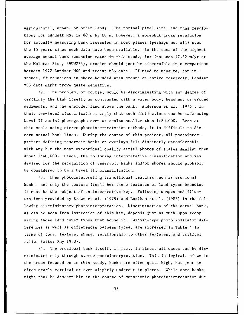
agricultural, urban, or other lands. The nominal pixel size, and thus resolu-
tion, for Landsat MSS is 80 m by 80 m, however, a somewhat gross resolution
for actually measuring bank recession in most places (perhaps not all) over
the 15 years since such data have been available. In the case of the highest
average annual bank recession rates in this study, for instance (7.32 m/yr at
the Molstad Site, 39DW234), erosion should just be discernible in a comparison
between 1972 Landsat MSS and recent MSS data. If used to measure, for in-
stance, fluctuations in shore-bounded area around an entire reservoir, Landsat
MSS data might prove quite sensitive.
72. The problem, of course, would be discriminating with any degree of
certainty the bank itself, as contrasted with a water body, beaches, or eroded
sediments, and the uneroded land above the bank. Anderson et al. (1976), in
their two-level classification, imply that such distinctions can be made using
Level II aerial photographs even at scales smaller than 1:80,000. Even at
this scale using stereo photointerpretation methods, it is difficult to dis-
cern actual bank lines. During the course of this project, all photointer-
preters defining reservoir banks on overlays felt distinctly uncomfortable
with any but the most exceptional quality aerial photos of scales smaller than
about 1:40,000. Hence, the following interpretative classification and key
devised for the recognition of reservoir banks and/or shores should probably
be considered to be a Level III classification.
73. When photointerpreting transitional features such as erosional
banks, not only the feature itself but those features of land types bounding
it must be the subject of an interpretive key. Following usages and illus-
trations provided by Brown et al. (1979) and Loelkes et al. (1983) is the fol-
lowing discriminatory photointerpretation. Discrimination of the actual bank,
as can be seen from inspection of this key, depends just as much upon recog-
nizing those land cover types that bound it. Within-type photo indicator dif-
ferences as well as differences between types, are expressed in Table 4 in
terms of tone, texture, shape, relationship to other features, and vcrtical
relief (after Ray 1960).
74. The erosional bank itself, in fact, in almost all cases can be dis-
criminated only through stereo photointerpretation. This is logical, since in
the areas focused on in this study, banks are often quite high, but just as
often near'y vertical or even slightly undercut in places. While some banks
might thus be discernible in the course of monoscopic photointerpretation due
37

Table 4
Photointerpretive Key Developed for Discrimination of Erosional
Reservoir Banks along the Middle Missouri River
Photo Indicators Identified Feature
Water Surface
Tone Water surface is distinguishable primarily by photographictone and texture. Calm water surface is dark toned inboth black and white (where it is black) and color (black)to blue) aerial photos, while its tone in color infraredphotographs is determined by the amount of suspended sed-iments and varies from black to light blue.
Texture The photographic texture of the water surface is deter-mined by the regularity and definition of waves and theirorientation to incident sunlight. A very fine, regularwave texture is usually seen on all but the calmestsurfaces.
If incident sunlight is such that it reflects directlyinto the camera lens from the water surface, that surfaceor portions of it may appear to be the brightest object ina photographic scene, rather than very dark. Such a watersurface reflection is easily recognizable since it willnot occur in previous or subsequent frames along a flightline.
Shape The shape of the boundary of the water surface can varyfrom extremely smooth, in the case of shallowly slopingbeach or other shore contacts, to almost randomly ir-regular in small-scale photographs when it laps directlyagainst convoluted shorelines.
Relationship to In relation to other features, the water surface can beother features bounded by a beach, or alternatively it can impinge dir-
ectly upon a bank or upon a shore that does not displaya distinct vertical bank.
Vertical relief Stereoscopically viewed, the water surface is extremelyflat, to such an extent in fact that no vertical relief atall can be determined.
(Continued)
(Sheet I of 4)
38

Table 4 (Continued)
Photo Indicators Identified Feature
Beach
Tone Since, in the study area, beaches are uniformly composedof light colored, fine sediments, they are very light grayto white in tone on all photographic emulsions. Areas ofbeaches recently wetted by waves can be slightly darker intone than higher portions of the beach.
Texture Beaches themselves are extremely uniform, fine-to-indiscernible photographic texture. Due to the presenceof cobble- and boulder-size material on some of thebeaches along the main stem reservoirs, both photo tone(above) and texture will vary in these areas from those ofthe beach itself.
Shape Beach shape is usually smooth and straight or smoothlycurving on the lakeward edge, while its shape on theshoreward side is determined by bank shape.
Relationship to The relationship of a beach to other features is variableother features in that a beach is only visible if it is uncovered or only
slightly covered by the water surface. In cases of highwater, beaches are not visible.
Vertical relief Topographically, beaches are very low gradient, low enoughin most cases to be indiscernible under stereoscopicinterpretation.
Slumped Sediment
Tone Slumped sediment detached from a bank can fill a shortdistance between beach and bank, or if a beach is notpresent between the water surface and the bank. Slumpedsediment is generally of medium tone due to irregularitieswhich create slight shadow effects. Organic materials inslumped sediment may also contribute to a slightly darktone.
Texture The photographic texture of such sediment is visiblycoarser than that of the beach or water surface.
Shape Slumped sediment indicators are less regular in shape andoutline, particularly lakeward, than either water surface
Relationship to or beach indicators. Slumped sediment typically occurs inother features short segments along bank and occupies a relatively thin
strip between water and bank, or beach and bank.
(Continued)(Sheet 2 of 4)
39

Table 4 (Continued)
Photo Indicators Identified Feature
Slumped Sediment (Continued)
Vertical relief The vertical relief of slumped sediment is discerniblygreater than the water surface or beach, but its heightis less than that of the bank itself.
Erosional Bank
Tone The erosional bank, a feature of primary interest in thisstudy, it also perhaps the most difficult to discern. Itsphotographic tone--or more properly the tone of boundingshadow indicators--can in some places be sharply dark, butin other cases there may be virtually no tonal indication.If the bank is not strictly vertical, or if radial dis-placement allows the definition of the toe of the verticalbank, then the exposed face can be light in tone. If it_s composed of darker sediments, or rack (such asPierre Shale at 39DW234), it may however be medium to darkgray in tone.
Texture Such an exposed erosional bank face is also often of fineand uniform texture, although if of extremely convolutedshape, it can appear rougher in texture.
Shape In terms of shape, banks can range from long and uniformlystraight, to highly convoluted. In most cases viewed inthis study, straight banks also exhibited uniform vertical
Relationship to relief, while their convolutions--inundated relict drain-other features ages dissecting terrace edges--are less uniformly vertical
in relief, with shallower gradients.
Vertical relief It is in terms of their three-dimensional relief that ero-sional banks are best defined. Since the base-to-heightratio of stereo photographs with 60-percent overlap ex-aggerates vertical heights up to about seven times nor-mal, and since in the case of most erosional banks theseheights are considerable or at least abrupt in compari-son with surrounding surface, they are sharply visible andunambiguously determinable in most cases under a stereo-scope. It is difficult to understand how erosional banksin many cases can be mapped using only monoscopic inter-pretation, however.
(Continued)
(Sheet 3 of 4)
40
Table 4 (Concluded)
Photo Indicators Identified Feature
Shoreward Surface
Tone The shoreward surface is the surface found on the top sideof the erosional bank, away from the slump, beach, andwater surfaces that may be seen lakeward from it. Invirtually all cases in -,r study areas, at least portionsof the shoreward surface are covered by grassland andbrush throughout the years included in the aerial photo-graphs. In some cases, trees occur near the bank edge andobscure the bank for short distances. In nearly allcases, the photographic tone of the shoreward surface isdarker than beach or slumped sediments, but considerablylighter than either shadows under the bank, or the watersurface. For this reason, when no beach or slumped sedi-ment is present, even if the bank cannot be confidentlydiscerned, the abrupt boundary between shoreward surfaceand water surface can be defined.
Texture The shoreward surface's texture depends upon its vegeta-tive cover, as well as its topographic variations whichcatch shadow depending upon their orientation and the sunangle on the photo date. In the case of uniform grass orshrub cover on flat terrace surfaces, texture is fairlyuniform. Brush or trees, that in fact often grow differ-entially in cultural features (housepit depressions andfortification features) coarsen the shoreward surface'stexture.
Shape The shape of the shoreward surface is determined by itsinterface with the shape of the erosional bank or withthe waterline.
Vertical relief Topographically, the shoreward surface is in some casesremarkably level, while in other cases it varies consider-ably due to prereservoir topographic contours. In thecase of the Midipadi Butte study area in North Dakota(32DU2), for instance, the shoreward surface risesabruptly, beyond the actual erosional bank, at least 50 m.In some other cases, for instance at the Cable Site(39LM224) or Whistling Elk (39HU242), the shoreward sur-face is in most places almost totally level for some dis-tance inland.
(Sheet 4 of 4)
41

to shadow marks, most aerial mapping photographs are taken in midday. When
stereo pairs of aerial photographs, taken along a flight line with about a
60-percent overlap (as, in fact almost all mapping photos), are viewed on a
stereoscope, the vertical relief of the erosional bank is easily seen in
aerial photos of scales of about 1:40,000 or larger (in some cases, smaller-
scale photographs of high quality are useful as well).
Methods for Measurement of Bank Erosion
75. The methods we have incorporated in this research build upon those
developed for the National Park Service's Interagency Archeological Services
and outlined in a report entitled "Using Aerial Photographs to Measure the
Erosion of Archeological Sites" (Ebert and Lyons 1986). This publication was
initiated to provide National Park Service Personnel with a series of methods
to be used to measure erosional impacts to park archeological sites. It out-
lines ways that sequential, historical aerial photographs can be used for
measuring erosion of archeological sites in a simple manner.
Selection of study sites
76. The sites forming the basis of this study were selected from
25 sites designated at a meeting of Corps of Engineers archeologists in 1986
as being representative of erosionally endangered cultural resources along
Middle Missouri River reservoirs. The 12 study sites examined were chosen be-
cause they are representative of the erosional threats identified by Corps of
Engineers archeologists. These sites and their locations are shown in
Table 5. Details of the archeological significance of these sites, and the
perceived erosional threats to them, are given in the draft final report.
77. Laboratory methods. Building upon methods developed previously
(Ebert and Lyons 1986), the following methods were adapted for the measurement
of bank erosion at the 12 study sites:
a. Acquisition of aerial photographs. The first step in thisproject was the search for all available aerial photographs ofthe study sites. Inquiries were made of all applicable Federaland state sources for the areas in which the study sites werelocated; four major agencies were found to hold the aerialphotos covering the sites. These agencies, the aerial photo-graphic coverage located and used, and its scale, emulsion, andother characteristics are listed in Appendix A.
42

Table 5
Locations of the Study Sites
LegalSite Description Latitude Longitude
Nebraska
1) 25KX200 T33N R2W SEC 17 420 50'00" 970 34'00"
2) 25KX57 T33N R2W SEC 18 420 50'00" 970 34'00"
North Dakota
3) 32DIT2 T147N R19W SEC 1 470 35'44" 1020 13'00"
South Dakota
4) 39C06 T22N R30E SEC 22 450 51'00" 1000 23'30"
5) 39LM224 T1O7N R74W SEC 2 440 06'00" 990 40'50"
6) 39HU242 T109N R76W SEC 3 440 16'20" 990 57'45"
7) 39HU173 T112N R80W SEC 4&9 440 32'00" 1000 25'00"
8) 39BF44 T106N R71W SEC 15 430 59'20" 990 20'00"
9) 39ST235 T4N R33E SEC 13 440 18'30" 1000 06'00"
10) 39DW234 T17N R31E SEC 7 450 27'30" 1000 21'00"
11) 39WW15 T124N R79W SEC 32 450 31'00" 1000 25'00"
12) 39YK40 T93N R57W SEC 16 420 52'00" 970 35'45"
L. Compilation of base maps. Base maps at a scale of 1:10,000, agraphically manageable scale, were made by photomechanicallyenlarging US Geological Survey, 1:24,000-scale, 7-1/2-mintopographic quad sheets. Those sheets listed in Table 6 wereused for this purpose.
(1) Portions of these topographic sheets, containing the areaaround the site, a 2-km by 2-km square, and sufficientadditional area within which mapped details useful forphotographic control could be found, were enlarged ontofrosted mylar photographic film, each measuring 55 cm by55 cm. Map detail was screened at 60 percent of fullblack level in order to provide contrast between the mapdetails and later drafted shorelines.
(2) Also, it should be noted that the shorelines shown on thepublished US Geological Survey maps bear little or no re-lationships to actual water levels, shores, or banks. Inthe early stages of thiE research, the US GeologicalSurvey mapping office in Denver was contacted and asked
43

Table 6
USGS 7.5-mmn Topographic Quad Sheets Used
for Compiling Study Site Base Maps
Site USGS Quad Sheet
25KX57/200 Tabor SE, Nebraska-South Dakota 1968
32DU2 Twin Buttes, North Dakota 1967
39CO6 Kenel, South Dakota 1967
39WW15 Mobridge, South Dakota 1967
39YK40 Tabor SE, Nebraska-South Dakota 1968
39BF44 Bedashosha Lake, South Dakota 1974
39HU173 Okobojo SW, South Dakota 1973
39LM224 Lower Brule, South Dakota 1966
39DW234 Moreau, South Dakota 1968
39ST235 Rosseau, South Dakota 1973
39HU242 DeGray, South Dakota 1973
about the meaning of what appeared to be water levels orshorelines on several of the maps. In some cases, thenominal average pool level was used as the waterline; inother cases, the water level on the day on which the aer-ial photographs from which the map was compiled was drawn.
(3) Paper copies of the base maps, with drafted shorelinesdetermined from aerial photographs, were provided in thedraft copy of this report.
c. Control location. Next, the enlarged mylar base maps and eachset of aerial photographs were inspected to determine appropri-ate photo control points. Requirements for such control pointsare that they are visible on both the aerial photographs andthe base maps. These points were to be used to match and, dur-ing overlay projection, for dimensions. In most cases, atleast three identifiable control points--such features as theintersections of roads, small stock tanks, or buildings--could
be found on maps and aerial photographs. At some of the studysites including 39CO6 and 32DU2, however, finding matching con-trol points on maps and each photograph proved difficult due tothe lack of map detail. In these cases, a method that might bedescribed as using serial control was used in which identifi-able trees, shrubs, and other photovisible features were usedas control to match consecutive photointerpretive overlays toone another. Although such features rarely persist throughoutthe entire photo time sequence, sufficient points to allowmatching from one photo date to another can be found.
44

d. Formulation of a photointerpretive key. Photointerpretation,while it may be thought of to some extent as an art, must beguided by replicable interpretive rules or keys to beconsistent. To formulate such a photointerpretive key, theaerial photographs of the study sites were first preliminarilyinspected using a mirror stereoscope. A key specifying tonal,textural, and contextual factors allowing the discrimination ofwater surface, beach, slumped sediment, erosional banks, andshoreward surface was compiled. This key is included inTable 4 following a discussion of aerial photointerpretive map-ping of shores and banks.
e. Photointerpretation and overlay mapping. Using the photointer-pretative key, each date of aerial photographs was interpretedusing a Topcon mirror stereoscope with 1.8-, 3.0-, and 6.0-power magnification (Figure 2). During photointerpretation, atransparent mylar overlay was superimposed atop one of thephotographs of the stereo pair, and secured to that photo withdrafting tape. The locations of control points were thenmarked with a 4x0 rapidograph and acetate ink. Next, thephotointerpreter carefully traced a 2-km segment of bank line,centered on the study site and visible in stereo on the aerialphotographs. In cases where more than two aerial photos werenecessary to view the 2-km bank line segment, the overlay wasfixed to the central photographs in the necessary series sothat it would not be moved or repositioned. Stereo photointer-pretation is invaluable in identifying banks from aerial
Figure 2. Mirror stereoscope with an x-y tracking attachment
45

photographs because of the relief cues the operator can see.One of our concerns early in this stage was that the width ofthe rapidograph line would constitute a source of error.
(1) A 6x0 rapidograph was experimented with, but it cloggedafter only a few minutes of use.
(2) A 4x0 rapidograph seemed to be the best compromise betweenpracticality and line width; the 0.18-mm-wide ink linemade by the tip of this pen would, it was calculated, havea scaled width of 3.60 m on a 1:20,000-scale photograph.
After a bit of consideration, however, a means was devised tomake this a nonproblem: it was decided to use the edge of theline to define the bank, rather than its center. Using thisdrafting method, any size pen would be perfectly acceptable.
f. Projection of bank lines to base map scale. Each photointer-pretive overlay was next projected to 1:10,000 scale using aMap-O-Graph opaque projector with a special flat field lens.This was accomplished by matching chosen photo control pointsagainst their corresponding locations on the 1:10,000-scalebase map and redrafting the bank line at the base map scale(Figure 3).
. Definition of transects and measurement. A series of tran-sects along which measurements were to be made was constructedon the base map sheet. These transects were oriented perpen-dicular to the slope of the landscape at the point they inter-sected the earliest interpreted reservoir bank and were spaceda scaled distance of 100 m apart (1 cm apart on the 1:10,000-scale base map) at that point. The transects were oriented inthis manner primarily to help answer the question of whetherthe apparent bank recession being measured was due simply tovariations in reservoir pool levels rather than actual erosion.Upon analysis and further consideration, this possible problemseems relatively insignificant in our measurements, as dis-cussed later at greater length. Twenty-one transects weredefined for each site, with one intersect (No. 11) centered onthe archeological site itself, and ten intersects spaced 100 mapart on each side of the archeological site. The earliestinterpreted bank line was used as a baseline from which to makemeasurements to consecutive bank lines. After each interpre-tive overlay was matched and drafted onto the base map, thedistance between it and the baseline bank was measured, alongeach of the 21 transects, using digital calipers (Figure 4).Measurements were made to the nearest 0.01 mm; the FowlerMax-Cal calipers used have a nominal accuracy of 0.03 mm, whichscales to 0.03 m at the 1:10,000-scale map.
46

Figure 3. Projecting interpreted bank lines toscale and rectification with a Map-O-Graph opaque
projector
Sources and Magnitude of Errors in Measurementsfrom Aerial Photographs
78. An assessment of the possible sources and amounts of error in the
photointerpretation and mapping methods used to study bank recession along the
2 km reaches of shoreline is facilitated by a breakdown of error into two
basic types. The first of these is the inherent error. Such errors are not
occasioned by the specific measurements made here but are already contained
within the data sources and devices used in making those measurements. Inher-
ent errors which must be considered in this project include errors contained
in the aerial photographs, in maps used for control, and in the projection and
measurement devices used to actually make the measurements. Inherent errors
can e empirically estimated at some level, based on geometric, statistical,
and engineering parameters.
47

Figure 4. The measurement of distances between bank lines alongtransects with digital calipers
79. Another type of error affecting any measurement is the operational
error. Operational errors are those arising from the actual process of making
the specific measurements at hand. Operational errors depend upon the indi-
viduals making measurements. In this research, such errors would include the
variation introduced in interpreting the positions of bank lines, errors in
rectification and control matching during projection, variations in measure-
ment technique using calipers, etc., and some errors due to human decisions
such as at what level of precision one will carry out computer or other analy-
ses. Operational errors depend, then, on situationally and personally unique
factors of measurement and cannot really be estimated fully.
80. For this reason, nqost assessments of errors entailed in interpret-
ing, mapping, and measuring spatial data from aerial photographs focus solely
on inherent errors. Gatto and Doe (1983), in considering errors that might
affect their measurements of bank recession at northern Corps of Engineers
reservoirs, cite inherent errors in aerial photographs as most important, in-
cluding "...scale variations due to camera lens distortions and aircraft alti-
tude changes..." and "...radial, relief and tilt distortions...." Gatto and
48

Doe also found, as we did when trying to map specific archeological sites,
that measurements within small test areas are increasingly difficult as the
scale of the aerial photographs used becomes smaller. Errors (both inherent
and human) of the same basic magnitude in measurement from smaller-scale
photographs represent a greater proportion of the total measurement than in
larger-scale photos. Gatto and Doe (1983) adopted a rule-of-thumb for
accepting or rejecting measurements based on Tanner's (1978) concept of the
MMD. The MMD represents a confidence measure as a distance below which one
cannot, it is assumed, reliably measure from aerial photograph. If a measure-
ment they compared between two aerial photographs of different dates was less
than the combined MMD of both photographs or if it indicated that the bank
moved outward toward the reservoir, that measurement was not represented as an
absolute value but rather a range of values.
81. Millsop (1985) also explicitly used Tanner's MMD method to define
the level of precision to which he measured from historical aerial photographs
in his bank recession research along the shores of Lake Sakakawea. Millsop's
(1985) distance measurements were made from aerial photographs with a divider
and an engineers' scale to:
...the nearest 0.21 mm. This corresponds approximately to thestrict limit of measurement which the human eye can accuratelymeasure, as defined by Tanner (1978)...
82. In measuring patterns of Atlantic and Gulf of Mexico coastal
shoreline and island erosion and change using sequential historical aerial
photographs, Dolan et al. (1980), Shabica et al. (1984), and Dolan and Hayden
(1983) have calculated and estimated the extent of measurement errors, using a
number of methods. Correcting their error figures for the 1:5,000 scale at
which their photographs were interpreted onto base maps during projection,
they calculate such factors as inherent photo resolution limit of 0.02 m,
photo blur translating to 0.01 to 0.15 m, and the precision of the digitizer
used to trace high waterlines translating to 1.25 m (Dolan et al. 1980). A
much larger error in these measurements is occasioned by the difficulty of
matching control features on photographs with the base maps, estimated by
Dolan and Hayden (1983) to be approximately a 10-m ground distance. "The com-
bined error of all measurement steps was calculated with a maximum value of
12.85-m ground distance, although it is commonly on the order of 5 m" (Shabica
et al. 1984). Another source of inherent error that must be taken into
49

account in any procedure requiring the matching of photographs to maps for
control and rectification purposes is that error inherent in the maps
themselves. National Map Accuracy Standards published by the Office of
Management and Budget as a guide to acceptable government maps are in reality
somewhat difficult to interpret. As reproduced for photogrammetrists in the
American Society of Photogrammetry's Manual of Photogrammetry (Slama 1980),
they require the following:
a. Horizontal accuracy. For maps on publication scales largerthan 1:20,000, not more than 10 percent of the points testedshall be in error by more than 1/30 in.; for maps on publica-tion scales of 1:20,000 or smaller, not more than 10 percent ofthe points tested shall be in error by more than 1/50 in. Thelimits of horizontal accuracy shall apply in all cases to posi-tions of well defined points only. Well defined points arethose that are easily visible or recoverable on the ground,such as bench marks; property boundary monuments; intersectionsof roads, etc.; and corners of large buildings or structures.
b. Vertical accuracy. As applied to contour maps on all publica-tion scales, not more than 10 percent of the elevations testedshall be in error by more than one-half of the contour inter-val. This means that at a map scale of 1:24,000, the scalefrom which our base maps (and the maps used by Dolan et al.(1980) and the other references cited) were compiled, at least90 percent of well defined points must be accurate to within adistance of 40 ft, or 12.9 m. Ten percent of such points canbe in error greater than this distance; this is level of accur-acy to which the USGS and their mapping contractors strive.Map magnification, luckily, will not increase this error. Lessfortunately, this means that if only well defined points areused for control matching, the inherent map error in accuracyof control matching that can be expected may be as great as thesum of the other inherent and operational errors estimated bythe authors of this report. An error of nearly 25 m in con-trolled mapping, the sum of these errors, would be fatal in7:.ost bank recession measurements from aertal photographs ofwhich these authors are aware.
83. A few points can be made in an argument for still being able to
accept the results of this and other bank recession measurements made from
historical and sequential aerial photographs. This argument requires parti-
tioning the error or faithfulness of measurements into two categories somewhat
differently than the inherent versus operational dichotomy detailed above.
Measurements can also be thought of as having properties of both accuracy and
precision.
a. Accuracy is the faithfulness of a measurement to the realworld; this is the property of measurements dealt with in the
50

National Map Accuracy Standards (Slama 1980). They can betested against the real world, and are in this sense comparablefor the most part with inherent errors.
b. Precision refers to the repeatability of measurements, withrespect to one another. The precision of measurements dependslargely upon the abilities of the individual making those mea-surements, and the inherent error of the actual measuringdevice--dividers and scales, or digitizers, or digital calipersin the case of this research. Practically, the inherent errorsof measurement devices are very small compared to the errors inprecision that people make.
84. In the case of the measurements upon which the research reported
here are based, lack of accuracy when compared to maps is in some cases quite
noticeable. This is especially true where aerial photographs exhibit consid-
erable relief and thus inherent radial displacement and scale errors. This is
demonstrated by the lack of close correspondence between the mapped contours
of base maps and bank line measurements at 39DU2, our site with the greatest
relief differences (see the maps for 39DU2 in the appendices).
85. It is the relative distance between controlled representations of
bank lines that are being measured between, however, rather than their corre-
spondences with the base maps. The base maps are used actually to provide
only consistent control points, rather than (necessarily) accurate control
points. Unfortunately, precision errors (comprised mostly of operation
errors) are not possible to estimate, since they depend not only upon the in-
dividual, but the conditions under which the measurements are made as well.
An individual's precision of measurement can vary with factors as mundane as
amount of sleep and feelings at the time the measurements are made. Control
of these conditions over time would be impossible.
86. Such measurements will be consistent, however, if they are made at
the same time, and under the same conditions for the measurement instrument
operator. Although three such operators made the measurements in the case of
this research, all of the measurements for sequential shorelines for each site
were made within a short period of time (during one measurement session). In
experiments with the repeated measurement of small distances using digital
calipers, one of the authors, Ebert, usually averaged within I to 5 percent in
terms of precision or repeatability. What is more, most inherent error can be
estimated only in terms of a plus-or-minus error. This means that, for in-
stance, the measurement precision and accuracy of a digital caliper device
such as that used in this research, for example, be 0.03 mm less or greater
51

than the actual distance. It would vary around the true distance in both
directions during measurements, and during a large number of measurements this
two-way error between measurements would tend to compensate for itself. It
can be considered, in many instances, to be a form of self-correcting noise
rather than a real problem.
52

PART III: DATA ANALYSIS AND CONCLUSIONS
Bank Erosion: Causes, Processes, and Variables
87. Bank erosion, its causes, and its effects on our environment and
landform are not just topics of recent interest. A classical treatment of the
forms which lakeshore landforms take and the processes which give rise to such
features by the geomorphological pioneer G. K. Gilbert (1884) is still one of
the most complete descriptive treatments of such phenomena. Building on the
premise that "In shore sculpture the agent of erosion is the wave..." Gilbert
(1884) explains that the significant type of wave in this process is the wind
wave proper, existing during the continuance of the wind; the swell, which
continues after the wind has ceased, is far less important in bank and shore
erosion. While the wave is the chief agent, it is in turn influenced in its
energy and ability to erode sediments, and the effects upon sediments, by many
factors. These include the depth and shape of near offshore slope, the height
of wave crest, the nature of undertow which removes eroded sediments, the type
of sediment being eroded. Gilbert's primary illustration of the variability
of wave-cut landforms based on different combinations of these causes focuses
on cliffs, wave-cut terraces, beaches, barriers, and other littoral features
apparent around ancient, abandoned lakes such as those on the margins of the
Plains of San Augustin in New Mexico.
88. Reservoir bank and shore erosion, of which Gilbert probably had
few illustrations in 1884, is similar in many ways to that on oceans and natu-
ral lakes, but there are important differences as well. Reservoirs create a
unique erosional situation in that their impoundments create erosional shores
on slopes previously unaffected by lacustrine processes, causing immediate and
accelerated erosion and sedimentation (Lawson 1985). Upon reservoir filling,
flooding or almost instantaneous shoreline erosion causes the loss of vegeta-
tion which may have protected sediments for millennia. Hydrologic conditions
are altered through the modification of the water table and of the previous
drainage system, by overbank flooding, and by fluctuation of reservoir water
levels within a variable zone. Rapid injection of sediment into the water
column adjacent to the shoreline causes offshore features to form quickly,
modifying the erosional regime. While water level variations of different time
scales may be equivalent in their effects per unit time, they are quite likely
53

of widely different predictability; seiche-induced water level differences,
for instance, could only be predicted or measured given a large, dense network
of recording stations.
Time scales
89. The factors which influence reservoir-related erosion can be
attributed to several time scales. Water levels in many reservoirs are manip-
ulated on a short-term basis, often on the order of a few days, according to
the purposes for which the reservoir system was built. Other short-term dif-
ferences in erosion can be caused by weather, and wind and barometric pressure
differences, for instance, can cause water levels to differ from place to
place on a single reservoir (seiche). Long-term fluctuations in water level
at reservoirs result from changes in climatic parameters, droughts for in-
stance, for several years or more. Bridging the periods between these are
seasonal fluctuations, which cause periodic water level fluctuations (Lawson
1985). Water level fluctuations are of course important in determining the
nature of bank and shore erosion on reservoirs, because they determine which
areas or sediments wave erosion reaches and affects.
Morphology
90. Shore morphology is another area in which reservoirs differ from
most natural shores. Reservoirs usually have an elongated shape, with greater
shoreline development (ratio of shoreline length to circumference of a circle
with the same area as the pool) (Lawson 1985); i.e., reservoir shores are
often convoluted, irregular, and complex. Factors affecting erosion in reser-
voirs can therefore be expected to vary significantly from place to place,
even over short distances. Reservoirs are deepest near dams, whereas natural
lakes are deepest in their centers, also enhancing spatial variability in ero-
sion along reservoir shores. The geotechnical properties of sediments along
reservoirs therefore will vary along their length, as well.
Equilibrium of shorelines
91. Newly created reservoir shores are immediately in disequilibrium
with their new lacustrine environment, and are thus highly unstable. The
length of time required to reach equilibrium will vary, because of the factors
just described, from reach to reach in many larger reservoirs. Although it is
tempting to think that shorelines in some places may reach equilibrium
quickly, some of the results of the present study show that apparently this
has not happened at our study sites in more than 30 years. The complexity
54

of the different components of shorezones, and therefore the difficulty of
assessing the factors that affect its shape and evolution (Dean and Maurer
1984; Bruun and Schwartz 1985; Dietz 1963) are compounded in reservoirs by
often great short- and medium-term changes in pool level, which constantly
change the identity of the shore zone profile (Lawson 1985). Specifically,
profiles of eroding reservoir margins often differ from typical natural
coastal profiles in having prominent, abrupt bluffs adjacent to a fore-
shortened beach profile. In many cases, a backshore zone is entirely absent,
with the waterline lying at or above the bluff toe. Natural lakeshore pro-
cesses and predictions may not, therefore, be completely appropriate analogs
for characterizing reservoir shores, and since large reservoirs are a rela-
tively recent phenomenon, the behavior of their shores is poorly understood.
Reservoir shore processes may in fact include many factors in common with
riverbank erosion, such as meander geometry, in an unknown combination with
lakeshore processes (Warren 1987).
92. Numerous processes, as well as factors which account for their
intensity and occurrence, interact to cause reservoir bluff or beach erosion
and subsequent shoreline recession. According to Lawson (1985), "No single
process or parameter uniquely accounts for erosion or recession of a bank or
bluff."
93. A recent summary prepared at CRREL of processes and phenomena
affecting bank erosion at northern-latitude reservoirs (Gatto and Doe 1983)
illustrates the complexity of these factors (Table 7, Figure 5).
94. The variables that any study incorporates in an attempt to explain
and predict a phenomena of interest, of course, vary with the objectives of
that study. A discussion of variables significant in explaining and pre-
dicting reservoir bank erosion germane to this study is presented by Millsop
(1985), who conducted studies above Garrison Dam at Lake Sakakawea in North
Dakota to assess the reasons that bank erosion there showed little sign of
reaching equilibrium since the filling of that reservoir.
95. Millsop (1985), in agreement with Gilbert (1884), observes that the
primary cause of reservoir bank erosion is waves. The effects that waves have
on banks, and hence the types and amounts of erosion and bank recession they
cause, are in turn dependent upon many measurable factors or variables. In
large northern reservoirs such as Lake Sakakawea, as well as the other lakes
considered in this study, important variables include: reservoir pool levels;
55

Table 7
Processes of Reservoir Bank Erosion and Contributing
Factors (Gatto and Doe 1983)
FrozenPerennially Seasonally Unfrozen
Frost wedgingFrost heavingIce wedgingThermoerosional niching and fallingGround-ice slumping
----- Ice lenses----------------------------- Ice scour ------------------------------ Ice push------------------------------- Ice pile-up---------------------------- Ice shelving--------------------------- Ice cover let down--------------------- Ice rafting---------------------------- Snow erosion--------------------------- Thawed soil slides----------------
-Positive pore-water pressure ---------------------------------- ---Groundwater piping--------------------
-------------------Chemical weathering---------------------------------------------------- Waves-------------------------------------------------- ------Currents-----------------------------
------------------- Water level fluctuations--------------------................... ------- Wind-------------------------------------------------- -------Falling Trees-------------------------------------- --- Man-induced erosion----------------------------------- -------Debris Sliding----------------------------------------- ------- Sloughing---------------------------------- - - Bank sediment characteristics------------------------- ----- Biological Factors-------------------
------------------------------ Sheet Flow----------------------------- Rill erosion- --------------------------- Gully erosion
---------------------------- Raindrop impact------------------------------- Landslides------------------------------- Earth fall------------------------------------ Slumps
56

PATTERNED GROUND WN
LAYER' ..
ICE WDGESFLOODEDICE W DG ESIC E C O V ER
THERMOEROSIONAL a m m m ~ m m
NICHE!WAVES
Figure 5. Bank erosion processes and bank characteristics contributingto erosion at northern reservoirs (from Gatto and Doe 1983)
wind velocity, direction, and duration; bank orientation; bank geology; bank
form; vegetation cover; the existence of natural riprap, beaches, or other
sheltering structure; and offshore bathymetry. "Activating factors" (Millsop
1985) include the actions of ice on shores (Gatto 1982b, 1984c), slumping or
bank failure of various types, and rainfall and overland water flows. These
variables or factors and their own dependent variables are as Millsop (1985)
summarized in Table 8.
96. To assess the various contributions and interactions of these vari-
ables, Millsop (1985) made measurements of bank recession--his "independent
variable"--over a 4-year period using measurements at pins on the ground, and
over longer historical periods using aerial photographs. He compared bank
erosion rates and trends in those rates with bank profiles measured on the
ground, wind, pool level data, evidence of overland water flows, precipita-
tion, ground water (measured with piezometers), the frost-thaw cycle (measured
through direct observation as well as frost tubes and thermographs), and the
nature of bank sediments (using field and laboratory measures).
57

Table 8
"Activating Factors" and Associated Dependent Variables Recognized
and Measured at Lake Sakakawea, ND (after Millsop 1985)
Activating Factor Dependent Variables
Wave Erosion Bank orientation, geology andgeometry; natural rip-rap andvegetative cover; offshoreprofile; offshore islands; poollevels; wind direction, strength,and duration.
Overland Erosion Preexisting moisture condition;(Rainsplash and Runoff) bank orientation, geology and
geometry; vegetative cover;precipitation intensity, dura-tion, and direction.
Ground Water Bank geology and geometry;topography; precipitation and
snowmelt amounts; pool levelfluctuations.
Frost-Thaw Preexisting moisture condition;bank orientation, geology andgeometry; vegetative cover;frost rate, depth, and duration;volume and concentration of ice;freeze-thaw cycles; rate of thaw;snowmelt amounts.
Lake Ice-shove Bank orientation, geology andgeometry; pool level; degree ofice cracking and refreezing; windstrength, duration, and
direction.
Vibration Location, intensity, and(man-made, wave-induced or duration.storm-induced)
97. Most bank erosion, Millsop (1985) concludes, occurs through the
process of bank failure or shear. Types of bank shear movements include falls
of overhanging masses (cantilever failure), topples or forward tilts, slides
(transitional or rotational), lateral spreads, and flows. Most shear events
are combinations of these types.
Wave action
98. Millsop's (1985) analyses illustrated that wave action is the
dominant erosional process at Lake Sakakawea, as it is on natural lakes in
58

that area (Reid 1985). Wind-driven waves undercut banks during high water,
bank shear occurs causing sediment collapse when water levels lower and sedi-
ments dry, and sediment is then removed at moderate to high-water levels.
Natural rip-rap or sheltering factors, rainfall, and overland erosion are of
very minor importance there due to the dry climate, which is the case at all
of the reservoirs studied here as well. Ground water, too, is relatively
unimportant except that related to reservoir levels. Frost-thaw cycles can
also be significant causes of bank failure but affect primarily jointed
bedrock. These cycles are less important in homogeneous fine-grained sedi-
ments similar to those found at the archeological sites upon which this study
focuses. Bank disturbance by human and animal activity are also acknowledged
as important in some places. Human activity is also noted in this study as
being an important, if difficult to control for (in both scientific and legal
terms), variable. This human activity occurs at the archeological sites in
this study in two forms: the effects caused by past human activity (i.e.
differences between archeological and culturally unaffected sediments), and by
present-day archeological looting. Not considered here are waves induced by
reservoir navigation; even in heavily navigated reservoirs, vessel induced
waves probably account for only about 5 percent of bank erosion (Gatto 1984c).
Bank erosion processes
99. Erosional processes observed and measured during this research are
also attributable, on an ultimate level, to the action of waves, affected pri-
marily by their energy and their effects on different portions of the beach/
bank profile due to fluctuations in reservoir pool levels. During periods of
higher water level, bank profiles are cut to the vertical in fine-grained,
homogeneous sediments, or less often undercut. When levels lower, shears of
these vertical banks result in topples or forward tilts (Figure 6), as well as
less consolidated flows (Figure 7). Sheared or slumped material is then re-
moved by further wave and current action.
100. An observed factor which may aggravate wave action in some cases,
or ameliorate it in others, is the existence along many reservoir shores of
tremendous amounts of often massive driftwood logs derived from the Missouri
River Valley forests which are now submerged (Figure 8). These now-dead trees
apparently float to the surface continuously, and batter against shores during
storms; it may be however, that they also offer an element of shoreline pro-
tection under certain conditions. Though the interaction of driftwood with
59

Figure 6. Large blocks of sediment shearing from the bank at theJones Village Site, 39CA3
Figure 7. Sediments recently collapsed probably due to topple or cantileverfailure of jointed silty sediments at the Jones Village Site, 39CAI
60

Figure 8. Large numbers of huge driftwood logs pound againstshores during storms, exacerbating bank erosion
winter ice is not known, the two will probably continue to be participants in
the shore system of Missouri River reservoirs for many decades.
101. Subsurface soil liquidity and resultant shear failures caused by
thawing and freezing are a common feature not only along reservoir shores in
the area (Figure 9), but also on slopes not immediately adjacent to reservoirs
or their banks, as illustrated by crazily tilting fenceposts, especially in
the Big Bend area of South Dakota (Figure 10).
102. In some areas, biological and cultural agents form what may be an
important subset of mechanical factors disturbing the integrity and thus
increasing the susceptibility of bank sediments to shear failure. While plant
cover and roots may increase the competence of sediments, our study sites are
covered almost entirely by grass cover with shallow root systems; this makes
overland water flows and rill erosion almost nonexistent, but has little
effect on resistance to bank sediment slump and removal. Birds and animals
burrow into banks, and may help cause bank failures (Figure 11). Another sort
of "biological burrowing" that may be quite significant, particularly because
it occurs only at archeological sites, is caused by illegal artifact looting
61

Figure 9. Successive shear failures, probably caused byfreezing and thawing processes
Figure 10. Slippage of surface soil layers during thawing causes
fenceposts in the Big Bend area to tilt in a downslope direction
62

'lit
Figure 11. Birds and burrowing mammals can weaken banks, facilitatingcollapse, while plant roots strengthen near-surface sediments
(Figure 12). Looters remove astonishingly large amounts of sediment and
undermine banks very effectively at some sites, and this activity occurs year
after year. Illegal artifact collectiing, then, poses a double threat to cul-
tural resources. This is one cause of bank erosion that would be relatively
easy to combat and control (Site 39C06).
Variables and measures
103. The variables recorded in this study were designed to meet analy-
tical goals outlined earlier in this report, specifically: (a) to allow the
measurement and description of bank recession amounts and rates through time
at the study sites, (b) to facilitate the identification of major processes
and factors influencing bank erosion at each study site, and in general in the
study area, and (c) to illustrate approaches that might be productive in
modeling bank erosion and predicting its future course at the study sites as
well as along the shores of Missouri River reservoirs in general. At the same
time, another somewhat more operational goal or consideration in this research
was to avoid overcomplicating our analyses at this developmental stage. The
scope of work for this research was written to include, for the most part,
63
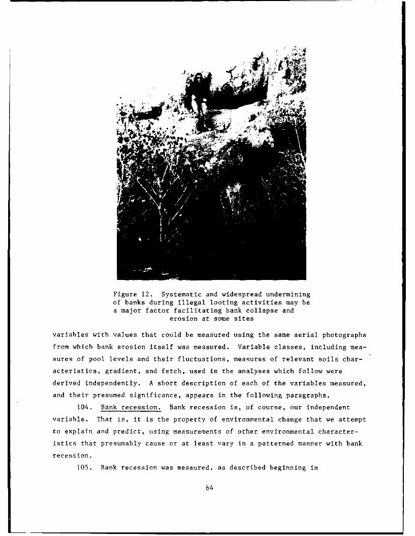
Figure 12. Systematic and widespread underminingof banks during illegal looting activities may bea major factor facilitating bank collapse and
erosion at some sites
variables with values that could be measured using the same aerial photographs
from which bank erosion itself was measured. Variable classes, including mea-
sures of pool levels and their fluctuations, measures of relevant soils char-
acteristics, gradient, and fetch, used in the analyses which follow were
derived independently. A short description of each of the variables measured,
and their presumed significance, appears in the following paragraphs.
104. Bank recession. Bank recession is, of course, our independent
variable. That is, it is the property of environmental change that we attempt
to explain and predict, using measurements of other environmental character-
istics that presumably cause or at least vary in a patterned manner with bank
recession.
105. Bank recession was measured, as described beginning in
64
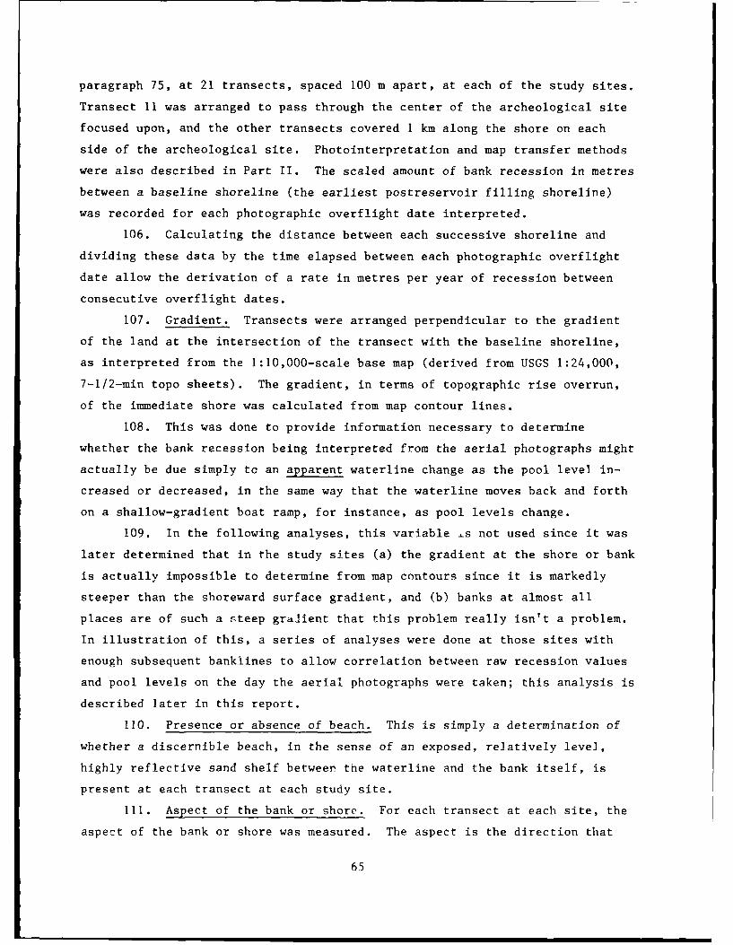
paragraph 75, at 21 transects, spaced 100 m apart, at each of the study sites.
Transect 11 was arranged to pass through the center of the archeological site
focused upon, and the other transects covered I km along the shore on each
side of the archeological site. Photointerpretation and map transfer methods
were also described in Part II. The scaled amount of bank recession in metres
between a baseline shoreline (the earliest postreservoir filling shoreline)
was recorded for each photographic overflight date interpreted.
106. Calculating the distance between each successive shoreline and
dividing these data by the time elapsed between each photographic overflight
date allow the derivation of a rate in metres per year of recession between
consecutive overflight dates.
107. Gradient. Transects were arranged perpendicular to the gradient
of the land at the intersection of the transect with the baseline shoreline,
as interpreted from the 1:10,000-scale base map (derived from USGS 1:24,000,
7-1/2-min topo sheets). The gradient, in terms of topographic rise overrun,
of the immediate shore was calculated from map contour lines.
108. This was done to provide information necessary to determine
whether the bank recession being interpreted from the aerial photographs might
actually be due simply to an apparent waterline change as the pool level in-
creased or decreased, in the same way that the waterline moves back and forth
on a shallow-gradient boat ramp, for instance, as pool levels change.
109. In the following analyses, this variable s not used since it was
later determined that in the study sites (a) the gradient at the shore or bank
is actually impossible to determine from map contours since it is markedly
steeper than the shoreward surface gradient, and (b) banks at almost all
places are of such a steep gralient that this problem really isn't a problem.
In illustration of this, a series of analyses were done at those sites with
enough subsequent banklines to allow correlation between raw recession values
and pool levels on the day the aerial photographs were taken; this analysis is
described later in this report.
110. Presence or absence of beach. This is simply a determination of
whether a discernible beach, in the sense of an exposed, relatively level,
highly reflective sand shelf between the waterline and the bank itself, is
present at each transect at each study site.
111. Aspect of the bank or shore. For each transect at each site, the
aspect of the bank or shore was measured. The aspect is the direction that
65

the shore faces, expressed in terms of the angle in degrees clockwise from
north of a line normal to (that is, perpendicular to a tangent at) each tran-
sect. Aspect was measured because it is an indicator of the wind direction
that should create waves most directly affecting bank or shore erosion at each
transect.
112. Fetch. Fetch is a measure of the distance over which wind-driven
waves originate, and is therefore indicative of the energy of wind-driven
waves. Waves driven farther by the wind are larger and stronger. Another way
of thinking of fetch is that a small fetch means that a bank or shore is more
sheltered.
113. Fetch was measured in kilometers to a resolution of 0.1 km in
three directions from the intercept of each transect at each site with the
shore after Phillipps (1986). The first fetch direction measured was shore-
normal, i.e. perpendicular to a tangent to the shore at each transect. Fetch
distances at angles of 45 deg both right and left of the shore-normal fetch
were also measured. This was done because winds are not always, of course,
shore-normal and are variable about a dominant direction over even short
periods. It also allows an assessment of the shelteredness of the shore at
each transect, which might not be apparent if, for instance, it was located at
the end of a narrow cove.
114. Pool levels and their fluctuation. In the foregoing discussion of
bank erosion factors and processes, one variable identified by previous rc-
searchers was the extent of pool levels and their fluctuation. Although pool
level on the aerial photo date could perhaps be measured from aerial photo-
graphs (although there would be problems with scale and resolution), pool
level and its dynamics between the photo dates, in the periods when bank ero-
sion was actually taking place, obviously cannot.
115. Pool level data are of course carefully collected at high (as
often as hourly) resolution. They present a serious data reduction problem.
What is more, our study sites were located at different places on the reser-
voirs, while pool levels are recorded at the dams themselves.
116. In order to comply with our goal of keeping the present analyses
relatively simple, but to still have general measures of the pool dynamics of
reservoirs between t-he aerial photo dates, three gross measurements were made
from graphs appearing in Plate No. 3 in the Corps of Engineers' "1986-1987
Missouri River Main Stem Reservoirs Annual Operating Plan and Summary of
66
Actual 1985-1986 Operations," prepared by the Missouri River Reservoir ControlCenter in Omaha. These graphs include pool elevations in feet above mean sea
level for the years 1955 through 1986. These graphs are presented here asFigures 13 and 14. These data served at the baqis for measurement of the
temporal, pool-level variables used in regression analysis.
117. From these graphs, the maximum and minimum pool levels that
1630 1530
1620 I 1620
1610 1610I,\
600 1 600
590 - - -590
f5a - - - 580
570 2 L-570560 j- 1560
- - -I i -, J155S1550 t T 1550
,Z1540 J 1540
IlU 1530 ----- 530> Ii ,520
1 5 2 0co 510----
1510 5]0
1 I350 ON 1 ' i E 1 , ; ,, 3800
,L 370 . .. -+-
'350 1350zo 1340 fl340
1330 L , 330
>I320 . . 320i, I I I ! ii : ,-LJ -~-- I I 320
LL 1310 - 10
300 -1-- -100±.., Ih±I L 2
FORT RANDALL1220 T12
f210 - -~ <II - KiI 1210
1 200 200
1 190+ f f90
55 57 59 6 3' 3 5 b' ' ) ' '5 , 7 ' 8 83 e5CALENDAR "rEAR;AVINS POTNT
Figure 13. Simplified pool levels for Oahe, Fort Randall,and Cavins Point reservoirs
67

I I I I II I I I II ll
_j 70 1870
l5_ 1850
0 - -40 1840< 130 1,2111
_T F1o1820
LUJU 810 - 1810
o 80 4A o800
z I0 1780 1780
1770 :1770
>1 760 1760
1L :7 50 1750
Figure 14. Lake Sakakawea pool level through time
occurred between each aerial photograph date for which bank recession was mea-
sured at each site were estimated to a resolution of I m. The difference be-tween maximum and minimum pool level for each period between photo dates wascalculated as well. Finally, a pool fluctuation index was determined bycounting pool level peaks, separated by valleys of pool level minima, between
each photo date.
118. Soils properties. A final class of independent data with assumedrelevance to bank erosion that we attempted to measure was soils properties.
Soils classifications developed by the USDA's SCS are available for mostcounties in the study area but are derived primarily for agricultural pur-poses; these classifications are thus also almost always difficult to relate
to most nonagricultural investigations. The SCS soils classifications arebased on the description of a suite of properties for each of a number ofsoils associations and series, so that even continuous variables are brokendown by nominal soils unit categories, and the data generally available forsuch variables are given as ranges typical of each soils unit. For many pur-poses, then, such variables may be simplified to such an extent as to be prac-tically worthless for explanatory purposes at high spatial resolution.
119. What is more, the agriculturally oriented classifications mappedby the SCS pertain in almost all cases to surface properties of soils and theareas they cover, extending in most cases to depths of 60 in. or less. Obvi-ously, this takes into account only a portion of the variability in sediments
that comprise banks at most of the study sites.
68

120. Nonetheless, inspection of the variability in bank recession rates
and the SCS soils descriptions between and within the study sites does indi-
cate that differences in soils are perhaps of some explanatory importance.
Rather than attempt to use nominal classes, three classes of continuous vari-
ables incorporated in these soils descriptions which seemed to vary the most
with measured bank recession rates were extracted from published and unpub-
lished SCS data for the counties containing our scudy sites for which it was
available. These variables are:
a. Erosion factor (K). This is one of six factors used in theUniversal Soil Loss Equation to predict the average annualrate of soil loss by sheet and rill erosion in tons per acreper year. K is based primarily on percentage of silt, sand,and organic matter (up to 4 percent) and on soil structure andpermeability. Values of K range from 0.05 to 0.69 and indi-cate the susceptibility of a soil to sheet and rill erosion;the higher the value, the more susceptible is a soil to sucherosion by water.
b. Liquid limit and plasticity index. These measures are de-rived from the Atterberg limits, and indicate the plasticitycharacteristics of a soil. They are based by the SCS on testdata from the survey area or from nearby areas and on fieldexamination.
121. These index measures are given as ranges for each soils class in
SCS country soils descriptions. Some soils units contain estimates of all
three indexes, and some contain only one or two indexes.
122. To determine these variable values, the soil unit intersected by
each measurement transect at each site was first identified. The range of
values contained within each soils description was then averaged, to derive a
single, central value, and these were then coded for each transect in each
site.
Measurements, Variables, and Data Structure
123. At the end of the last section, a summary of the types of data
interpreted and measured in the course of this research was given. The term
variable is used in most scientific research in at least two diffirent ways.
The actual measurements taken during research are often called variables, but
the term can be used in another sense as well--the analytical variables in-
cluded in attempts to model or explain phenomena. The phenomena to be ex-
plained are dependent variables, while those that the scientist believes to
69

be causal, or to affect, or at least vary with the dependent variables are
independent variables.
Problem orientationand dependent variables
124. The focus of this research, and the analyses set forth are rates
of reservoir bank recession as they vary in space and in time. For the inde-
pendent variable, RATE, there are at least three basic scales or magnitudes of
variation in space and time that are important to consider. These are:
a. The mean rate of bank recession at the site over the period ofrecord.
This rate is a site-specific average bank recession ratemeasured from the first or baseline bank date through thelatest bank date, averaged for all measurement transects or,alternatively, for any single measurement transect. It isaffected by both spatial and temporal variation within thesite as a whole. In the case of this research, this rate isfound by averaging the recession rates for each of the 21transects measured at each site, over the time of record.This rate is expected to differ to some extent from one siteto another due to a combination of site-specific variables,within-site spatial variation between transects, and varia-tions within each transect through time.
b. The variation in bank recession rates over space at each site.
This is the difference in bank recession rates throughoutthe time of record (between the first and last bank measured)among 100-m spaced transects at each site. Variation betweenaverage rates among transects at a site will be due to differ-ences in independent variables that do not vary through time,specifically bank orientation, fetch (a measure of sheltered-ness of each point on the bank), and the characteristics ofsoils or sediments as they vary between transects with each2-km stretch of bank line.
c. Variation in bank recession rates over time at each transect.
Measurement of bank recession using multiple sets ofsequential aerial photographs allows the breakdown of ratesinto time periods. These rates vary due to independent vari-ableL that change through time, or have different valueswithin the time periods between successive aerial photograph(and therefore bank measurement) dates. Such independentvariables include properties of the pool level at each reser-voir; these probably, however, interact in various ways withthe nontemporal independent variables at each site. Othernonmanageable independent temporal variables, such as theoccurrence of storms and local high winds that are difficultor impossible to measure for each site, probably also haveimportant effects in terms of variability in bank recessionover high-resolution time.
70

125. Dependent variables designed to represent each of these types and
scales of resolution are used in the analyses presented in this section.
These variables are:
a. A gross site-specific bank recession measure consists of theaverage of bank recession at all transects within each studysite over the total time period measured for that site. Thisrate is designated SRATE in the data structure.
b. A mean bank recession rate at each transect within the siteconsists of the total bank recession distance measured at eachtransect within each site. This distance is divided by thetotal time period represented between the first (baseline) andlast bank position measured. This rate is designated as TRATEin the data structure.
c. Bank recession rates for each transect in each site are mea-sured by dividing the difference between bank positions atsuccessive measurement (aerial photo) dates by the elapsedtime between each successive measurement date. This dependentvariable is designated RATE in the data structure.
Variables
126. The derivation, and assumed importance, of the independent vari-
ables measured from the aerial photographs, or by independent means, used in
the analyses presented here are described in the preceding paragraphs.
127. Measurement variables used to calculate dependent variables, along
with the dependent variables and the independent variables used in the analy-
ses presented here, are listed and summarized in Table 9.
Bank Recession Rates at Study Sires
SRATE, TRATE AND
RATE for individual sites
128. A first level of analysis is approached here through the presenta-
tion of simple tables and graphs for each site depicting SRATE, TRATE, and
RATE. Table 10 pi-sents site-averaged or SRATE values, along with their stan-
dard deviations (SD), and a summary of number of photo measurement dates used
and the first and last photo dates, for each of the 12 study sites. Sites are
arranged in order of bank recession rates, from highest to lowest. A review
of this table indicates that sites are being lost at a rate of about 2.5 m or
8 ft/yr. Although it may seem unrealistic to report rates to two decimal
places, it must be remembered that summary statistics presented in Table 10
represent rates averaged from a series of measurements; and, that in any case,
71

Table 9
Measurement, Dependent, and Independent Variables
Used in Analyses
ASPECT The direction, in compass degrees, that the bank at theintersection of each measurement transect faces. This is adirection perpendicular to the tangent of the bank at eachtransect, or normal to the bank
DATE The date at which each bankline was interpreted and betweenwhich distances between banks were measured
DISTDIF1 The distance between the baseline bank and the bank measuredat each date
DISTDIF2 The distance between a bank and the bank interpreted priorto the time at which each bank was defined
FETL The fetch distance (that is, the unimpeded water distance)in kilometres between the intersection of each transect withthe bank at an angle of 45 deg to the left of the normalfetch
FETR The fetch distance in kilometres at the intersection ofeach transect with the bank at an angle of 45 deg to theright of the normal fetch
FLUCT The number of peaks in pool level fluctuation countedbetween successive bank measurement dates
K Soil erodibility factor as described in the section above
LEVDIFFI The difference in pool level between the baseline (earliest)bank time measured, and the latest bank
LEVDIFF2 The difference in pool level between successive bankmeasurement dates through time
LEVEL The pool level above mean sea level on the date that theaerial photographs from which each bank measurement weretaken
LIQ Liquid retention index for soils, as described inparagraph 120b
NORFET Fetch distance in kilometres along a line normal to thebank at the intersection of each transect
(Continued)
72

Table 9 (Concluded)
PDIFF Absolute difference in metres between the maximum andminimum pool elevations occurring between successivephoto/measurement dates
PLAST Plasticity index for soils at each transect
PMAX Maximum pool level achieved at any time between successivephoto/measurement dates
PMIN Minimum pool level achieved at any time between successivephoto/measurement dates
POINT Numerical designator for each transect
RATE The rate of bank recession (expressed in metres per year)between two successive measurement dates for each transect.This is the distance between the two dates divided by thetime between these dates
SRATE The mean bank recession rate at each individual site,derived by averaging TRATE over all of the 21 transects ateach site
TRATE Mean bank recession rate (metres per year) at each transectfor the entire period of measurement. This is derived bydividing the distance between the first and the last datedbanklines for each transect by the elapsed time betweenthose two transects
73

Table 10
Overall Erosion Rates (SRATE) for Middle Missouri River Sites
Erosion RateNumber of Photo Date Mean SD
Site Photos First Last m/yr m/yr
39DW234 8 9-27-62 5-30-86 7.32 4.51
39C06 3 6-13-68 7-31-82 3.08 2.2239LM224 4 6-21-65 8-12-77 2.95 1.59
39BF44 7 8-5-55 5-31-86 2.59 0.9032DU2 3 5-25-66 10-18-85 2.44 1.2825KX57/200 6 6-18-57 9-8-78 2.37 2.4539HU242 5 6-17-68 6-3-83 2.33 1.0939ST235 6 6-17-68 6-3-83 2.23 0.49
39WW15 5 7-25-70 5-30-86 1.82 0.85
39HU173 4 6-18-68 5-31-86 0.60 0.7239YK40 8 6-28-56 5-23-83 0.41 0.60
inherent and operational errors affecting measurements have been acknowledged.
The decimal places by which measurements are reported are, of course, the con-
sequence of the physical process of measurement, and statistical operations
should not be taken simply as a reflection of accuracy or precision.
129. A few general observations should be made concerning SRATE's.
First, these rates are all well within the magnitude of bank erosion or reces-
sion rates made by other researchers measuring bank and shore erosion at man-
made reservoirs, as well as natural lakes and oceans cited previously in this
report. The sites with the highest SRATE's also exhibit the highest standard
deviations in rates over space, generally speaking. This means that the
variation between rates at transects within these sites is highest.
130. There is also a striking variation in SRATE's between sites; the
mean (average) SRATE among all of the study sites is 2.56 m/yr, with a stan-
dard deviation of 1.80 m/yr. Clearly, simply citing an average rate of bank
recession for archeological sites and their surrounding banks along Middle
Missouri reservoirs is not necessarily a completely workable strategy for pre-
dicting actual rates of erosion at any of them.
131. Tables and graphic representations of TRATE and RATE at individual
74

sites, as well as the distances and times used to calculate these variables,
are presented in Appendix B under the sections for each site. Specifically,
tables and graphs included for each site are:
a. A table of the scaled distances (in metres) between the sitebaseline and each measured bank line through time (DISTDIF1),by DATE.
b. A table of the scaled distances (in metres) between successivemeasured bank lines through time (DISTDIF2), by DATE.
c. A table showing elapsed time between DATE's, expressed indecimal years.
d. A table representing between-date bank recession rates inmetres per year.
e. A table showing bank recession rates averaged over the periodof record, or TRATE (i.e. between the baseline or first andthe last measured bank line) by transect at each site.
f. A graph showing the means and range (standard deviation) ofTRATE's for each transect.
A graph showing the mean of all RATE's (i.e. bank recessionrates at each transect for each time period measured, lumpedfor all transects through time.
132. While the various rates depicted for each site, and some of their
site-specific implications, will be discussed below, there is an important
general observation that must be made here. Some of the TRATE's in some of
the sites, as well as some of the site-averaged RATE's for successive dates,
exhibit means and ranges that appear to indicate that the banks have moved
outward into the reservoir, rather than uniformly receding in a shoreward
direction.
133. Strictly speaking, of course, true banks--that is, sediments con-
solidated prior to reservoir filling--cannot move in a poolward direction. In
the reservoir bank recession studies cited in the preceding paragraphs of this
report, for instance, Gatto and Doe (1983, 1987) and Millsop (1985), conven-
tions were adnpted to drop or disregard Ruch negative recession measurements.
134. In the analyses presented here, we will not adopt such a co-,en-
tion for a number of reasons. First, we feel that arbitrarily dropping such
values erodes the usefulness of calculating standard deviations for measure-
ments. Expressions of the variation of measurements, such as the standard
deviation, are intended to express the effects of measurement error among
other things. If there are inherent and/or operational errors in our measure-
ments, as described in paragraphs 78-86 of this report, then doctoring
75

measurements obscure these errors in accuracy and precision.
135. Perhaps more importantly, however, we would point out that, espe-
cially when multiple measurements of banks (such as at our 2-km stretches of
bank/shore surrounding each study site) are made, in contrast to simple point
measurements, the definition of banks and their characteristics may vary
within a study site. A characteristic of the overall banks surrounding study
sites on the reservoirs examined in this study is that these may vary from
high, steep banks of prominent headlands, to low banks (or essentially no
banks at all) in inlets formed by the flooding of prior drainages cutting
through terrace surfaces into the river valley itself. In other words, all
banks are not equal, particularly in terms of gradient.
136. Another possibility is that sediment buildup of some sort may
actually be taking place, causing the bank to appear to move toward the reser-
voir pool rather than away from it. This might be due to the creation of
beaches by alongshore currents, or the slumping of large blocks of sediment
from banks into the pool or onto the beach at different photo dates.
Study sites summary
137. Summary discussions of photointerpreted bank recession at each of
the 12 study sites presented refer to tables of scaled distances measured
between baselines and bank lines and between successive bank lines and bank
recession rates included in Appendix B. Periods of rapid bank recession and
the locations which have experienced the most rapid recession are discussed.
Site maps illustrating transect location and topography are available in the
draft final report.
a. Site 39BF44 is located on an eroding terrace immediately northof Wolf Creek and is the only site examined on Lake FrancisCase. The site contains three prehistoric occupational compo-nents including Plains Woodland, Initial Middle Missouri, andCoalescent components. Photographs from which shoreline mea-surements were made include seven sets of stereo pairs takenover a period spanning 30.9 years (Appendix B). Transects 1through 5 are situated along the west and southwest-facingshore of a peninsulalike area formed by the terrace betweenWolf and Crow Creeks. This point of land has experienced themost rapid rates of erosion. Transect 12, intersecting a lowlying west-southwest-faclng terrace immediately north of themouth of Wolf Creek, also has a high erosion rate. Consid-ering the entire overall recession distances for the 30-yearperiod of investigation, the average recession rate for alltransects was calculated at 2.58 m/yr. Average erosion ratesusing individual periods of observation range between less
76

than 1 m/yr to over 7 m/yr. As can be seen, transects 1through 5 and transect 12 have the highest overall measures ofaverage rate and standard deviation. The area of site shore-line is represented by transects 11, 12, and 13, each of whichexhibits moderately high recession rates. Periods of the mostrapid recession for these transects fall between 1969 and1973, 1981 and 1983, and 1983 and 1986 (Appendix B).
b. Site 39ST235 (Stony Point) is located on a level expanse ofterrace at the base of a series of steep bluffs bordering LakeSharpe and includes the remains of a Post-Contact Coalescentearth-lodge village and earlier Initial Middle Missouriremains. Field investigations reported the terrace conformsto the MT-2 landform described by Coogan and Irving (1959).The site is situated in the middle of the expanse of shorelineexamined between transects 9 and 11 on a bulging section ofterrace. Five sets of aerial photographs spanning a 15-yearperiod between the baseline date and 3 June 1983 were used tomeasure the recession rate (Appendix B). Translating dis-tances measured between photo dates into erosion rates, therates for the period preceding Sep 1968 are very high fortransects 1 through 9. Rates for succeeding periods aremoderate to low for these transects. Between 1972 and 1982,rates appear to be stabilized for most transects but riseagain for the period between 1982 and 1983, especially fortransects 11 through 21. Apart from aspect, transects Ithrough 9 differ from the others in that they are situated onSully-Sansarc complex soils. This soil complex is distin-guished by 9- to 25-percent slopes compared with 3- to9-percent slopes for soils along the remainder of the shore-line investigated. Differences in slope are not perceptibleat the scale of the USGS topographic quadrangle, but may ac-count in part for differences in erosion rate between transectlocations.
c. Site 32DU2 (Midipadi Butte Site) is located on a flat-toppedbutte which rises 50-m above the western shore of LakeSakakawea and includes house depression constructed in theperiod between A.D. 1781 and 1815 as well as Woodland Tradi-tion ceramic and lithic artifacts. The bank line defining theedge of the actual site at 32DU2 and its intersection with thewater line has a variable morphology. The slope of the banknear the edge of the mesatop is at an approximate 45-degangle, while it becomes progressively steep as it nears thewaterline.
(1) Photointerpretation illustrates that this steep butteface was present at the site prior to reservoir fillingand the effect of reservoir filling can be assessed byinspection of the aerial photographs taken on 5 Sep 1966(just after the filling of the reservoir) and 10 Oct1985. These illustrate a trend of the foreshortening ofthe horned peninsula upon which the mesa containing thesite is located, as well as the less pronounced but stillobvious collapse and retreat of the bank edge atop the
77

butte. If anything, the slope of the bank defining theoutside edge of the site itself has become more shallow,while still losing sediment. That 32DU2 is undergoingsignificant bank recession is obvious; the relationshipof this bank recession to independent variables affectedby wave dynamics may be more complex than in most of thestudy sites, however.
(2) Three sets of aerial photography spanning a period of19.5 years were examined to obtain edge recession data(Appendix B). Transects 6 and 11 intersect the north-western and southeastern corners of the butte and havethe highest erosion rates, 5.8 and 2.3 m, respectively.Highest rates for the intervening transects are less than2.7 m/yr. Mean rates for periods of observation rangefrom less than I to more than 5 m/yr. The negative ratesfor trarqect 7 may be attributable to slumping of thebutte edge during the period between 1982 and 1985. Atrend through time in overall cannot be accessed withonly two periods of observation.
d. Site 39LM224 (Cable Site) is located on a broad terrace whichextends north into Lake Sharpe. Cultural remains include anearth-lodge village attributed to the Extended Coalescent.The site is listed in the National Register of HistoricPlaces. The terrace surface is slightly indented along a lineparalleling and about 25 m from the shoreline. Bank recessiondistances are relatively great along this section of shore-line, averaging 2.94 m/yr between 1965 and 1977. Using abaseline date of 21 June 1965, total distance eroded exceeds100 m at several transects (Appendix B). Seven sets of aerialphotographs for the period been 1965 and 1984 were examined toobtain these measures of bank retreat, but average bank reces-sion listed in Table 10 (2.92 m/yr) could be calculated onlyfor the period prior to 1977. Transects 10, 11, and 12 inter-sect the site area and have overall measures of bank retreatof from 65 to 120 m for the period between 1965 and 1984.Compared with transects 11 and 12, transect 10 intersects thewestern edge of the terrace and has relatively high rates oferosion. Erosion rates through time begin with moderate ratesof about 4 m/yr for the period prior to 1969 and rise to over10 m/yr for the period prior to 1981. Rates then declineafter 1981, but negative rates indicated for the periods priorto 1982 and 1984 do not represent aggradation at the shore-line. The small scale of the 1984 photographs, 1:80,000, isprobably responsible for difficulty in interpreting the bankline on this date resulting in less precise measurement.Photograph scale does not explain the negative measurementsobtained with the 1982 photos. These are, however, within amore acceptable margin of interpretation error. It shouldalso be pointed out that if negative recession rates aredropped from tables presented in Appendix B, the overall meanerosion rates for transects at this site are increasedmarkedly. Transects 10, 11, and 12, for example, would have
78

erosion rates of 9.75, 5.24, and 5.27, respectively, if aver-aged for the periods between 1965 and 1981, rather than ratesof 5.61, 0.69, and 1.10, respectively.
e. Site 39WW15 (Travis 2 Site) is located to the west of a pointof land on the west side of a former tributary drainage to theMissouri River which now forms a small embayment. The siteincludes surface and subsurface artifact distributions alongthe east bank of Lake Oahe that contain projectile pointstypologically assigned to Paleoindian and Plain Archaic occu-pations. Shallow slopes (generally less than a 15-ft riseover a distance of 1,000 ft) characterize the entire shorelinewithin the study area. Differences in bank recession dis-tances among transects dates point to landform and gradient asmajor influences in recession rate at this site. Five sets ofaerial photographs taken between 1970 and 1986 were used tomeasure bank erosion at the site (Appendix B). On the firstphoto date, 25 July 1970, the point of land west of the smallembayment intersected by transect\ 14 is partially inundated.Pool level on this date measured 1,608.5 ft. A higher poolelevation on 30 May 1986 of 1,617.4 ft is responsible for thetotal submergence of the point on succeeding photographs. Thetotal recession distances as measured from the large-scale,high-quality 1986 photographs do indicate the largest reces-sion distances for transects 14 and 15 that border the embay-ment on the west and east, respectively. These areas alsohave the lowest gradients of any areas along the shoreline.The remainder of the shoreline investigated slopes to agreater degree, although no steep banks are present on theportion of the shoreline examined. Transects 8 through 13intersect the site and have total recession distances of from20 to almost 27 m. Averaging recession rate for periodsbetween photo dates, these distances translate into a littleover 1 m of bank erosion per year for transects 8 through 10.Transects 12 and 13 have slightly lower rates.
f. Site 39HU242 (Whistling Elk) is located on the east bank ofLake Sharpe. During a survey of this site by the Universityof Nebraska (Steinacher 1983), it was noted that extensiveerosion had taken place at this site, listed in the NationalRegister of Historic Places, since the time of its originalrecording in 1968. This shoreline erosion rcvealed evidenceof a buried Plains Village site consisting of an earth-lodgevillage surrounded by a fortification ditch. Bank recessionrates measured over the period between 1968 and 1983 (AppendixB). Transects 8 through 11 intersect the site shoreline andhave low to moderate rates for this section of shoreline.Rates are initially quite high for transects I through 7 tothe west of the site, while transects 12 through 21 evidencehigh rates for the period between 1981 and 1983. Averagerecession rates for transects 8 through 11 are close to thoseobserved by Toom for the period between 1979 and 1983. Toomand Picha (1984) observed between 1/2 and 2 m of bank erosionper year, while mean rates measured from aerial photographsare between about 1/2 to I m/yr. Rates also appear to
79
increase through time averaging about 2 m/yr prior to 1981,increasing to almost 5 m/yr for the period between 1981 and1983.
g. Site 39YK40 (Jazz and Jill Site) is located in a high bank ofthe Lesterville stream approximately 400 m upstream from theentrance of this drainage into Lewis and Clark Lake. It con-sists of five fire areas situated 15 m below the presentground surface and from 5 to 15 m above the stream bottom(Blakeslee and O'Shea 1983). Since the site is located in theexposed bank of a tributary drainage to the Missouri River, itis not susceptible to reservoir shoreline erosion. This areais not visible on aerial photographs due to heavy forestcover, and degree of recession was, therefore, not investi-gated at this location. The reservoir shoreline was investi-gated, however, to determine if the Lesterville stream wassusceptible to flooding during periods of high reservoir poolelevation. Accordingly, the study area was centered at themouth of the drainage on which the site is located, and bankrecession distances were measured for the reservoir shorelinefor the period between 1956 and 1983 (Appendix B). Tran-sects 8 through 11 are positioned around the entrance of thestream into the reservoir. Transects 8 and 9, intersectingthe shallow gradient of a terrace on the downstream side ofthe entrance, evidence the greatest initial recession dis-tances between photo dates. Transects 10 and 11, intersectinga high bluff on the opposite side of the stream, show compara-tively little erosion. Average erosion rates for these tran-sects are quite low and have little variability. Rates forperiods between photograph dates appear to be generally lowand relatively uniform. At no time does the Lestervilledrainage itself become flooded. Thus, if reservoir pool ele-vation does not exceed 1,208.3 ft. the maximum elevation forthe period studied, the site should not be affected by reser-voir shoreline erosion.
h. Sites 25KX57 and 25KX200 (Weigand) consists ot a dense depositof ceramics and lithics extending for a distance of 50 m alongthe east bank if Weigand Creek and 30 to 35 m along tho westbank of the creek and shore of Lewis and Claik Lake. fhe sitewas described as centered around the original bank of WejindCreek (Blakeslee and O'Shea 1983) and now extends into Lewisand Clark lake. Bank erosion measurements were made for theperiod betueen 1957 and 1978 (Appendix B). Transects 14and 15 intersect either side of the mouth of Weigand Creek andtransect 13 intersects the shore of Lewis and Clark Lake tothe west of the creek where 25KX57 is located. Transects 9,10, 11, and 12 intersect the shore of Lewis and Clark Lake tothe west of 25KX57 where 25KX200 is located. 25KX200 issituated on an elevated portion of terrace. After reservoirconstruction, this area formed a point of land extendinF intothe lake as do smaller and more culturallv disturbed areas oneither side of Weigand Creek. Transects 10, 11, 14, and 15,intersecting points of land formed by these terrace
80

extensions, evidence the greatest overall and between-photodate amounts of bank recession. Highest measures of bankrecession through time are indicated for transect 11. Tran-sects 9, 12, and 13 display an opposite pattern, one in whichthe shoreline is aggrading in shallow embayments on eitherside of the point intersected by transect 11. These patternsof shoreline erosion can be identified in the averaged reces-sion rates for periods between photo dates. Average rates ofbank recession in the site area are highest for transects 10,11, 14, and 15 and are lowest and actually negative for tran-sects 12 and 13. When compared between photo dates, bank ero-sion appears to have increased through time until 1978. Theprogress of shoreline recession and aggradation continues sothat by 1985 the former points of land have become reduced andembayments are ringed with wide beaches.
i. Site 39CO6 (Jake White Bull) is an Extended Middle Missourifortified earth-lodge village located on the east-facing slopeof the second terrace above the Missouri River. The site islisted in the National Register of Historic Places. Bankrecession was measured from a baseline bank on 13 June 1968using two sets of subsequent photographs (Appendix B). Por-tions of the shoreline with the largest bank recession dis-tances are located at points of land bordering tributarydrainages to Lake Oahe which are intersected by transects 15and 20. Recession rates are highest for the 8-year periodprior to 1976. Three transects, transects 5, 7, and 8, evi-dence negative distances or shoreward movement of Lhe bank forthe period between 1976 and 1982. Inspection of aerialphotography of these locations indicated that bank slumpage oneast/southeast-facing slopes may be primarily responsible forthese measurements. Recession rates averaged for the twoperiods investigated range between about 2 and 4 m/yr with theexception of transects 15, 20, and 5. Transects 15 and 20average about 7 and 9 m/yr, respectively. Transects 10through 14 intersect the site shoreline and have erosion ratesof between 1.8 and 4.3 m/yr. These measures are quite com-parable to the average of about 3 m/yr observed by Larson-Tibesar personnel for the period between 1975 and 1986(Sanders et al. 1987).
. Site 39DW234 (Molstad Site) is an Extended Coalescent earth-lodge village, a National Register property located on thewest bank of Lake Oah! on the secoia terrace above the formerMissouri River floodplain. The terrace forms a prominencebordered on the north, east, and south by Lake Oahe andunderlain by Cretaceous Pierre shales which are exposed in thebank directly below and to the north of the site. Shorelinerecession was measured using eight sets of aerial photographsand appears to have been quite rapid, initially. One reasonfor the high initial erosion rate is that the terrace belowthe one on which the site is located became completely inun-dated between 1962, the earliest photo date, and 1968. Afterthis period, recession rates are appreciablv lower. The
81
overall mean recession rate calculated for all transects is7.31 m/yr, the highest mean rate of any site studied. Areaswith very high erosion rates are situated to the north andsouth of the site where study transects intersect tributarydrainages. These sections of shoreline have erosion ratesfrom 5 to about 40 m/yr (Appendix B). Transect 11 intersectsthe shoreline in the vicinity of the site. Recession rateaveraged for all periods of observation is 9 m/yr for thistransect.
k. Site 39HU173 is situated on an extension of a broad upperterrace above the former floodplain of Spring Creek about2.5 km east of the former confluence of the creek with theMissouri River. This elongated section of terrace terminateson each end in a point formed by the former courses of tribu-tary drainages with Spring Creek. University of Nebraskainvestigations recorded 21 stone features, including 11 stonecircles, 7 rock clusters, 2 rock lines, and I rock cairn ten-tatively attributed to both Woodland and Plains Village groupsbased on two projectile point fragments recovered from surfacecontexts. Bank recession measurements were made using a base-line date of 18 June 1968 and three sets of aerial yhotographsspanning a period of about 18 years (Appendix B). Study tran-sects 6 through 17 intersect the site shoreline. Althoughbank erosion has taken place at the southeastern portion ofthe peninsula where transects 14 through 17 intersect theshoreline, the majority of the site shoreline has experiencedlittle erosion. The erosion that has taken place at thesoutheastern portion of the site is not uniform between obser-vation periods. Averaged photograph rates are well under1 m/yr. Average recession rates for periods between photo-graph dates is highest prior to 1973, an average of 1 m/yr,and falls to 0.11 and 0.64 m/yr for the periods prior to 1981and 1986, respectively.
Fieldwork
138. It is always desirable to check results or conclusions measured or
interpreted from one sort of data with an independent data source. In remote
sensing, this activity is often referred to as ground truth checking, implying
that information gleaned from aerial photos must be proven by seeing it on the
ground. Of course, actually being on the ground is not always necessary;
interpretations made from one date or type of aerial photographs can also be
supported by similar observations made from another set of aerial photographs.
In one sense, this is a property built into any project involving the use of
sequential, historical aerial photographs.
139. In many ways, in fact, the truth of at least some kinds of mea-
surements of change from sequential photographs are difficult or impossible to
82

check in any specific way. The reservoir bank changes upon which this re-
search focused are of this nature, for the bank lines imaged on the historical
aerial photos are of course no longer there, and one cannot go back, find
them, and measure them on the ground. Neither can contemporary ground mea-
surements made on existing banks, nor short-term measurements of bank reces-
sion, really serve to confirm measurements of historical change.
140. It was reasoned, however, that it should be possible to make mea-
surements of portions of bank lines at a sample of the sites studied here on
the ground, and compare them with our historical data to at least support the
consistency of these measures over time. A field check of a sample of the
study sites would also allow ground photographs characterizing bank conditions
to be taken, and allow supportive observations to be made. With these goals
in mind, a three-week field reconnaissance was undertaken between 28 Sep and
18 Oct 1987. Sites visited are listed in Table 11.
Table 11
Missouri River Sites Fieldwork
28 Sep to 18 Oct 1987
Oct 02 32DU2Oct 03-08 39DW234, 39WW15, 39CO6Oct 09-10 39LM224Oct 13 39YK40Oct 14-15 25KK57/200
141. The chief activity at each site visited, with the exception of
39YK40 and 25KX57/200, was mapping a portion of the bank using a Wilde T-16
theodolite equipped with a Lietz RED-2 Electronic Distance Meter (EDM). After
a suitable instrument location was established, from which a portion of the
bank line centered on the actual site could be covered, angles and distances
to a range-pole mounted prism were shot in. Shots were taken at points which
would allow the resolution of what were judged to be significant changes in
the linearity of the bank. Control points that could be used to match mapped
bank lines to the 1:10,000 base maps used to control the photointcLpreteO
overlays, described in paragraph 77, were also shot in.
142. Vertical angles and slope distances were transformed to horizontal
distances and elevation differences, and these data were used to plot the por-
tions of bank line measured at each site to 1:10,000 scale using Generic CADD
83

Version 3.0 (Logitech, Inc.). These bank lines were then transferred to the
1:10,000 scale base maps, and distances between those 100-m transects covered
by the EDM-mapped banks and the last aerial photo-mapped bank line were mea-
sured. The EDM-mapped bank line segments are shown on the 1:10,000-scale map
copies attached to draft copies of this report. Bank erosion rates were deter-
mined by averaging scaled, measured distances so determined by time elapsed
between the last photo measurement and the EDM measurements. Bank recession
rates determined in this manner are compared with overall, aerial photo-
measured rates in Table 12. In all cases, the EDM-mapped bank line sediments
fell either behind or on the last photographically interpreted bank line.
Table 12
Comparisons of EDM-Measured and Aerial Photo-Measured
Bank Recession Rates
EDM-Number of Elapsed Measured Overall Photo- Recent Photo-
Site Transects Years Rate Measured Rate Measured Rate
39C06 5 5.191 1.95 m/yr 3.08 m/yr 1.63 m/yr (1976-1982)SD = 2.22 SD = 3.42
39WW15 12 1.348 3.19 m/yr 1.82 m/yr 2.32 m/yr (1981-1986)SD = 0.85 SD = 2.07
39LM224 3 2.946 2.57 m/yr 2.95 m/yr 8.44 m/yr (1981-1977)SD = 1.59 SD = 5.52
39DW234 5 1.356 1.95 m/yr 7.32 m/yr 1.34 m/yr (1982-1986)SD = 4.51 SD = 3.69
39HU242 3 4.360 1.16 m/yr 2.33 m/yr 4.74 m/yr (1981-1983)SD = 1.09 SD = 3.26
143. At site 32DU2, an EDM map of the edge of the mesatop containing
the site was made, but due to the nature of the topography, this cannot be
compared in any direct way with the bank line there at 1:10,000 scale. A
further discussion of the reasons for this problem, and comparisons of the EDM
map with two previous site-boundary maps at 32DU2, appears in the draft report
in the section for this site.
144. Site 39YK40 does not lie along the shore of Lewis and Clark Lake,
but is located between 500 m and I km from its shore in a small, steep-sided
valley unaffected by the reservoir pool. Since the aerial photo measurements
were made along the reservoir shore, no comparisons could be made. The
84

erosional situation at 39YK40 is discussed in its section in the appendix of
the draft report.
145. Site 25KX57/200 was not EDM-mapped because the entirety of its
unstabilized shoreline was inaccessible and, in fact, could not be defined
when this site was visited. The waterline, at that time at least and probably
for most of its existence (to judge from the historical aerial photographs),
consisted of water underlying a thick mat of reeds and other vegetation. Mea-
surements of the bank line and its recession at this site made in any manner
may, for this reason, be difficult to interpret.
146. For those sites where compariscns can be made, however, three of
the EDM-measured rates are within or almost within one standard deviation of
the aerial photo-measured rates. For 39LM224, the two rates are within a few
percent of one another. The EDM-measured rate at 39WW15 seems quite high com-
pared with the aerial photo-measured rates, although it is still almost within
one standard deviation. Verbal reports from local archeologists indicate,
however, that high water in the summer and fall of 1986 may have caused above
average erosional effects. This seeming inconsistency, then, might serve as a
reminder that some of the most significant bank recession may be caused by
short-term events, and that averages can be misleading. The elapsed time be-
tween the last photo-measured date and the EDM measurements is short, only
about 15 months. Using a shorter measurement period, the rate calculated for
the period between 1981 and 1986 is quite comparable to the EDM-measured rate.
147. The EDM-measured recession rate at 39DW234, where the highest ero-
sion rates were photographically measured, is low. Elapsed time between EDM
measurement and the latest photointerpreted bank line at this site is also
only about 15 months, however. The very rapid initial recession rate between
1962 and 1968 during which the terrace below the one on which the site is
located was inundated contributes is a significant fashion to the high overall
photointerpreted rate at this site. The erosion rate calculated for the
period between 1982 and 1986, 1.34 m/yr, is quite comparable to the EDM-
measured rate.
Analysis of Pool Levels and Apparent Bank Recession
148. In an attempt to analyze variation in the characteristics of banks
that might lead to "negative" measurements of apparent bank erosion, we first
85

tried to measure the gradient at the intersection of each transect with the
bank. Our measurement transects were oriented perpendicular to the gradient,
as shown on the 1:5,000-scale base map enlargements. These enlargements were
made from 1:24,000-scale, 7.5-min USGS topographic quads, with contouz lines
at intervals of 10 to 20 ft.
149. Unfortunately, this contour resolution does not, in our opinion,
allow the accurate calculation of gradient at the critical point between the
reservoir pool and the surfaces containing archeological remains on Middle
Missouri reservoirs, given the topography of the terrace-reservoir system.
150. The following questions still remain, however. Is there, in the
case of some transects within some or all of the study sites, a relationship
between pool levels and apparent bank recession or the lack thereof? If the
gradient (however unmeasurable) of the shore zone at a transect is sTallow,
and a true bank (i.e., a tall, vertical, or near-vertical sediment cross sec-
tion) is not present, might not an increase in pool level cause an apparent
shoreward shift in the bank and a decrease cause an apparent poolward shift,
without any real erosion or aggradation taking place?
151. It is important to examine the possible effects of pool level on
bank line recession. To examine this question further, pool elevation data
for each measurement (aerial photo) date for each of the study sites were
obtained from the US Army Engineer District, Omaha (the variable LEVEL in
Table 8). A series of correlation analyses were performed at those sites with
more than two photo measurement dates; variables used in these analyses were
DISTDIF2 (the distance that banks were measured to have changed between suc-
cessive photo dates), and LEVDIF2 (the difference in pool level between suc-
cessive photo dates). It was reasoned that if, indeed, pool level were influ-
encing the apparent distance between bank lines, these two variables would
show positive and significant correlations.
152. Of the 12 study sites, 9 had enough photo dates to accomplish such
corrclation analyses. The results are shown in Table 13. In this table, the
R (regression coefficient) values and their significance 1evels are shown.
For the nine sites analyzed in this way, there were 180 transects with suffi-
cient (no missing) data to be used in correlation analyses. For 105 of the
transects used in this analysis, R values were negative. Among the 180 with
sufficient data for these correlation analyses to be performed, there are 14
transects for which the correlation coefficients are significant at the 0.1
86

Table 13
Correlations of Between-Date Measurements (RATE) and Pool Levels
for Aerial Photo Dates, by Transect
Site 25KX57/200 Site 39WW15 Site 39HU173Transect R* p(R)** Transect R* p(R)** Transect R* p(R)**
1 -0.278 0.650 1 -0.295 0.704 12 0.766 0.131 2 23 -0.171 0.783 3 34 0.539 0.348 4 -0.273 0.726 45 -0.014 0.982 5 -0.762 0.247 56 -0.153 0.806 6 -0.085 0.914 67 0.167 0.787 7 0.224 0.775 7 -0.277 0.8208 -0.730 0.161 8 -0.121 0.879 89 -0.438 0.460 9 -0.550 0.449 9 -0.996 0.054
10 -0.376 0.532 10 0.219 0.780 10 0.424 0.72111 0.660 0.224 11 -0.276 0.723 1112 0.256 0.677 12 -0.782 0.216 12 0.905 0.27813 0.050 0.936 13 -0.727 0.272 13 -0.996 0.05414 0.543 0.344 14 -0.214 0.78 14 -0.917 0.26015 0.596 0.287 15 15 -0.299 0.80616 0.295 0.629 16 0.553 0.466 16 0.759 0.45017 -0.380 0.527 17 0.221 0.778 1718 -0.049 0.936 18 -0.067 0.932 18 0.999 0.00719 -0.056 0.927 19 19 0.350 0.77120 -0.264 0.667 20 -0.336 0.664 20 -0.419 0.72421 -0.094 0.879 21 -0.350 0.649 21
Site 39LM224 Site 39HU242 Site 39YK40Transect R* p(R)** Transect R* p(R)** Transect R* p(R)**
1 1 0.069 0.930 1 -0.599 0.152 -0.487 0.512 2 0.202 0.797 2 -0.089 0.843 0.817 0.046 3 -0.146 0.853 3 -0.284 0.534 -0.274 0.598 4 0.610 0.389 4 -0.198 0.665 0.011 0.982 5 0.008 0.991 5 0.282 0.536 -0.182 0.722 6 0.204 0.795 6 -0.010 0.987 0.485 0.504 7 -0.232 0.767 7 0.064 0.898 -0.421 0.405 8 -0.067 0.932 8 0.607 0.149 9 0.478 0.521 9 0.402 0.37
10 0.077 0.884 10 -0.246 0.753 10 -0.051 0.9111 -0.220 0.647 11 -0.442 0.557 11 0.238 0.6012 -0.318 0.538 12 0.958 0.041 12 -0.462 0.2913 0.069 0.895 13 0.144 0.855 13 -0.425 0.3414 -0.325 0.528 14 -0.693 0.306 14 -0.813 0.0215 -0.121 0.819 15 -0.175 0.825 15 -0.494 0.25
(Continued)
* R = Pearson's product moment coefficient.** p(R) = probability.
87
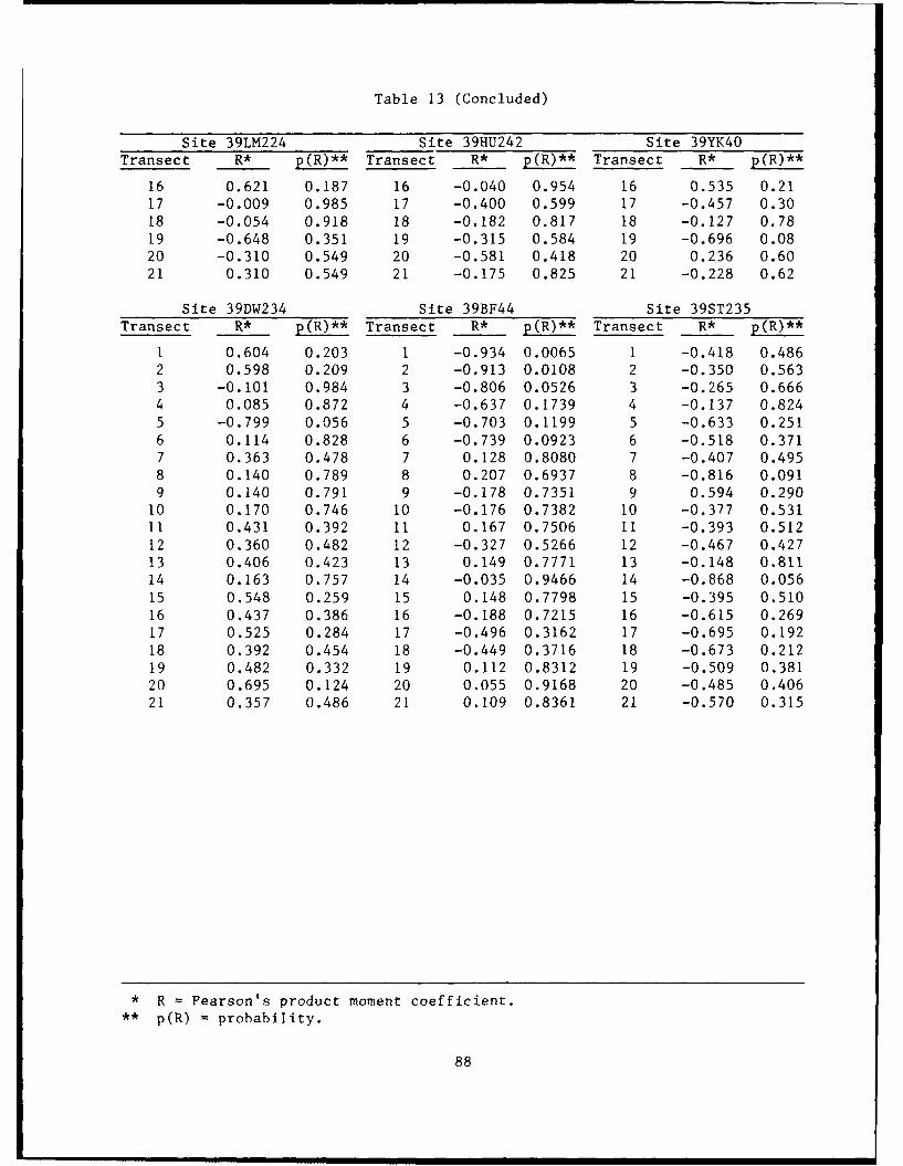
Table 13 (Concluded)
Site 39LM224 Site 39HU242 Site 39YK40Transect R* p(R)** Transect R* p(R)** Transect R* p(R)**
16 0.621 0.187 16 -0.040 0.954 16 0.535 0.2117 -0.009 0.985 17 -0.400 0.599 17 -0.457 0.3018 -0.054 0.918 18 -0.182 0.817 18 -0.127 0.7819 -0.648 0.351 19 -0.315 0.584 19 -0.696 0.0820 -0.310 0.549 20 -0.581 0.418 20 0.236 0.6021 0.310 0.549 21 -0.175 0.825 21 -0.228 0.62
Site 39DW234 Site 39BF44 Site 39ST235Transect R* p(R)** Transect R* p(R)** Transect R* p(R)**
1 0.604 0.203 1 -0.934 0.0065 1 -0.418 0.4862 0.598 0.209 2 -0.913 0.0108 2 -0.350 0.5633 -0.101 0.984 3 -0.806 0.0526 3 -0.265 0.6664 0.085 0.872 4 -0.637 0.1739 4 -0.137 0.8245 -0.799 0.056 5 -0.703 0.1199 5 -0.633 0.2516 0.114 0.828 6 -0.739 0.0923 6 -0.518 0.3717 0.363 0.478 7 0.128 0.8080 7 -0.407 0.4958 0.140 0.789 8 0.207 0.6937 8 -0.816 0.0919 0.140 0.791 9 -0.178 0.7351 9 0.594 0.290
10 0.170 0.746 10 -0.176 0.7382 10 -0.377 0.53111 0.431 0.392 11 0.167 0.7506 11 -0.393 0.51212 0.360 0.482 12 -0.327 0.5266 12 -0.467 0.42713 0.406 0.423 13 0.149 0.7771 13 -0.148 0.81114 0.163 0.757 14 -0.035 0.9466 14 -0.868 0.05615 0.548 0.259 15 0.148 0.7798 15 -0.395 0.51016 0.437 0.386 16 -0.188 0.7215 16 -0.615 0.26917 0.525 0.284 17 -0.496 0.3162 17 -0.695 0.19218 0.392 0.454 18 -0.449 0.3716 18 -0.673 0.21219 0.482 0.332 19 0.112 0.8312 19 -0.509 0.38120 0.695 0.124 20 0.055 0.9168 20 -0.485 0.40621 0.357 0.486 21 0.109 0.8361 21 -0.570 0.315
* R = Pearson's product moment coefficient.
** p(R) = probability.
88

level. Of the correlation coefficients for these 14 transects, 11 are nega-
tive. A negative correlation coefficient in this analysis signifies that as
the pool level increased, the apparent bank line moved poolward rather than
shoreward, or as the pool level decreased, the bank line moved shoreward.
153. This is essentially the opposite of what would be expected if pool
level were influencing apparent bank recession measurements. It may be that
bank slumping at some transects is causing the interpretation of poolward
movements; however, bank collapse following pool level decreases may also be
produced. Given the extremely small number of transects for which correla-
tions (negative or positive) are significant even at the 0.1 level (a very
liberal level of significance), it is likely that the appearance of poolward
measurements of bank erosion are due to random combinations of inherent and
operational errors.
Aspect and Bank Recession
154. All treatments of the causes of bank erosion and recession cited
previously in this report focused on the action of waves and wind as a primary
causal factor. People often speak of prevailing winds, but in practice the
relationships between wind speed, direction, and duration from place to place
are difficult to measure and characterize. Wind-rose graphs for a number of
weather recording stations in North Dakota, South Dakota, and Nebraska were
obtained from the US Department of Transportation for possible use in this
study, but reducing and interpreting these data proved too complex to be
incorporated here.
155. Instead, it was reasoned that if prevailing wind directions,
velocity, and durations were constant over time (an assumption that is possi-
bly valid given the 20+ year record at some of the study sites), and if, in
fact, wind direction, especially winds of high energy, are important in bank
recession rates, then the aspect and fetch of reservoir shorelines should vary
in a patterned way with bank recession rates.
156. As a prelirinary assessment of whether such patterning does in
fact exist, the general aspects of the study sites were examined in relation
to bank recession rates. The general aspect of each site was measured by the
perpendicular, facing poolward, of a line drawn from the shore intersect of
transect 1 to the shore intersect of transect 21 for each site. The
89

patterning of these general aspects of the study sites (that is, the direction
they generally face) is distinctive, to say the least. Because of the
northwest-to-southeast trend of almost all portions of the Missouri River
within North Dakota, South Dakota, and Nebraska, the study sites can be
divided into two very distinct groups: those facing between north and east
(aspect northeast) and those facing between south and west (aspect southwest).
A compass rose showing the general aspects of the study sites is presented in
Figure 15.
157. Tables 14 and 15 list the mean values of RATE's (bank recession
rates between consecutive bank measurements) and their standard deviations for
sites with northeast and southwest general aspects, respectively. An
N
039BF4 (26 39C06 (940)
Figure 15. Compass rose showing the general aspects of the study sites
9e

Table 14
Between-Date Rates (RATE) for Those Sites with
General Northeast (NE) Aspects
Mean HighDate Reservoir Site Rate* SD Low Rate** Ratet
18JUN1957 Lewis & Clark 25KX57/200 0.0000 0.0000 0.0000 0.00005AUG1964 Lewis & Clark 25KX57/200 1.7179 3.6658 -1.9479 5.38428APRI966 Lewis & Clark 25KX57/200 1.0721 5.8323 -4.7602 6.90404JUN1967 Oahe 39DW234 14.0972 15.2712 -1.1740 29.36813JUN1968 Oahe 39CO6 0.0000 0.0000 0.0000 0.00028JUN1968 Oahe 39DW234 50.4035 62.1659 -11.7624 112.56901SEP1968 Sharpe 39LM224 4.2932 4.3866 -0.0934 8.68001SEP1968 Sharpe 39ST235 24.8083 40.0762 -15.2679 64.88423JUL1969 Sharpe 39LM224 4.2278 10.4286 -6.2008 14.65604SEP1970 Lewis & Clark 25KX57/200 2.8472 6.0707 -3.2235 8.91815SEP1972 Lewis & Clark 25KX57/200 5.7646 10.1160 -4.3514 15.88104NOV1972 Sharpe 39ST235 2.1349 1.7052 0.4297 3.84018AUG1974 Oahe 39DW234 4.2234 4.4524 -0.2290 8.67609MAY1976 Oahe 39DW234 13.5265 15.1610 -1.6345 28.68810MAY1976 Sharpe 39ST235 0.6449 1.2888 -0.6439 1.93419JUN1976 Oahe 39CO6 4.1953 2.9810 1.2144 7.17612AUG1977 Sharpe 39LM224 2.2781 2.5868 -0.1087 4.86508SEP1978 Lewis & Clark 25KX57/200 2.0173 3.1975 -1.1802 5.21501SEP1981 Sharpe 39LM224 10.9761 5.1824 5.7937 16.159020CT1981 Oahe 39DW234 -0.6166 5.5802 -6.1967 4.96430JUL1982 Sakakawea 32DU2 1.3186 0.5619 0.7568 1.88131JuL1982 Oahe 39C06 1.6281 3.4154 -1.7873 5.04303SEP1982 Sharpe 39LM224 1.5567 7.9305 -6.3739 9.48703SEP1982 Sharpe 39ST235 0.2436 1.4381 -1.1945 1.68208SEP1982 Oahe 39DW234 2.6094 18.0490 -15.4396 20.65803JUN1983 Sharpe 39ST235 20.7444 12.0400 8.7044 32.78430OCT1984 Sharpe 39LM224 -3.2473 7.3645 -10.6118 4.117180CT1985 SakAkawea 32DU2 8.0590 6.9775 1.0815 15.03730MAY1986 Oahe 39DW234 1.3430 3.6925 -2.3495 5.035
* Mean rate is the mean value of RATE's (bank recession rates between
consecutive bank measurements) and their standard deviations.** Low rate is mean rate minus one standard deviation.
t High rate is mean rate plus one standard deviation.
91
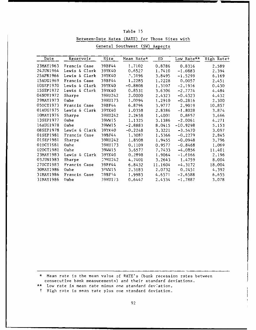
Table 15
Between-Date Rates (RATE) for Those Sites with
General Southwest (SW) Aspects
Date Reservoir Site Mean Rate* SD Low Rate** High Ratet
23MAY1963 Francis Case 39BF44 1.7102 0.8786 0.8316 2.58924JUN1964 Lewis & Clark 39YK40 0.6527 1.7410 -1.0883 2.39425APRI966 Lewis & Clark 39YK40 7.3196 3.8495 -1.5299 6.16915AUG1969 Francis Case 39BF44 1.2285 1.2228 0.0057 2.45110SEP1970 Lewis & Clark 39YK40 -0.8808 1.3107 -2.1916 0.43015SEP1972 Lewis & Clark 39YK40 0.8531 3.6306 -2.7774 4.48404NOV1972 Sharpe 39HU242 2.0000 2.4323 -0.4323 4.43229MAY1973 Oahe 39HU173 1.0094 1.2910 -0.2816 2.300050CT1973 Francis Case 39BF44 6.8796 3.9777 2.9019 10.857O1AUG1975 Lewis & Clark 39YK40 1.0358 2.8386 -1.8028 3.87410MAY1976 Sharpe 39HU242 2.2658 1.4001 0.8657 3.66613SEP1977 Oahe 39WW15 1.1325 3.1386 -2.0061 4.27116AUG1978 Oahe 39WW15 -2.8883 8.0415 -10.9298 5.15308SEP1978 Lewis & Clark 39YK40 -0.2248 3.3221 -3.5470 3.09701SEP1981 Francis Case 39BF44 1.3087 1.5366 -0.227q 2.84501SEP1981 Sharpe 39HU242 1.8508 1.9455 -0.0948 3.79601OCT1981 Oahe 39HU173 0.1109 0.9577 -0.8468 1.069020CT1981 Oahe 39WW15 3.6577 7.7433 -4.0856 11.40123MAY1983 Lewis & Clark 39YK40 0.2898 1.9064 -1.6166 2.19603JUN1983 Sharpe 39HU242 4.7401 3.2643 1.4759 8.004270CT1983 Francis Case 39BF44 6.8432 11.1604 -4.3172 18.00430MAY1986 Oahe 39%W15 2.3183 2.0732 0.2451 4.39231MAY1986 Francis Case 39BF't4 1.9983 4.6571 -2.6588 6.65531MAY1986 Oahe 39HU173 0.6447 2.4334 -1.7887 3.078
* Mean rate is the mean value of RATE's (bank recession rates between
consecutive bank measurements) and their standard deviations.** Low rate is mean rate minus one standard deviation.t High rate is mean rate plus one standard deviation.
92

inspection of these tables shows that the highest mean rates for sites with
general aspects within the northeast quadrant are an order of magnitude
greater than the high rates for those sites generally facing southwest. Wind
direction, then, is an important factor in predicting episodes during which
high bank recession rates occur and sites and transects where high rates occur
as well.
Multiple Regression Analysis
158. Multiple regression analysis is a procedure which is useful both
for identifying the relative contributions of suspected independent variables
on a dependent variable, and for predicting different future values of a
dependent variable on the basis of a number of independent variables. It is
incorporated in the analyses here with both of those goals in mind.
159. Two very different kinds of independent variables are incorporated
into the analyses described here. Some of the independent variables (see
Table 9 for a list and summary explanation--only the analytical variables are
considered here, not the measurement variables from which some analytical
variables were derived), as measured, are constant through time but vary in
space from place to place. These are:
ASPECT, FETL, FETR, K, LIQ, NORFET, PLAST
Other independent variables vary through time. These variables are:
FLUCT, PDIFF, PMAX, PMIN
160. Two dependent, analytical variables were designed for purposes of
the regression and other analyses presented here which could be examined in
the light of each of these groups of independent variables.
161. RATE is the rate of bank recession, in metres per year, derived
between two successive bank measurement dates. Each transect at each site has
more than one RATE; some transects have as many as seven RATE's. The time
periods associated with RATE measures each have their own values of FLUCT,
DIFF, PMAX, AND PMIN. To each of these RATE time segments can also be
assigned values for the nontemporal independent variables, although these are
93

constant within sites, and within reservoirs, so their inclusion into regres-
sions using RATE as a dependent variable would probably overpower and obscure
the correlation with temporal variables. Regression analysis of the variable
RATE with FLUCT, PDIFF, PMAX, and PMIN were designed to attempt to explain the
variation of bank recession rate over time.
162. TRATE is the bank recession rate, expressed In metres per year,
between the earliest and latest measured bank lines at each transect. One
transect has only one TRATE. For this reason, it is not meaningful to assign
values of the temporal independent variables to TRATE's; that is, there is no
variation through time for TRATE's, thus no potential correlation with
temporal variables. Regression analyses of the variable TRATE with ASPECT,
FETL, FETR, K, LIQ, NORFET, and PLAST were designed to examine the relation-
ship between differences in bank recession rate from place to place, rather
than changes in rate through time.
Regression methods
163. All of the statistical analyses described here were performed
using the statistical analysis system (SAS) for personal computers (SAS Insti-
tute 1985). The first step in each regression analysis, then, was determining
which variables, given the values of each to be incorporated into each regres-
sion analysis, were normally distributed. Following Millsop (1985), we re-
garded the distribution of values for a variable to be normal if its skewness
was between +1 and -1, and/or the Shapiro-Wilk Statistic, W, was 0.05 or
greater. Variables with values outside these ranges were regarded as non-
normal, and were not incorporated into the regression analyses. The distribu-
tion of values of a variable at one site, of course, might be nonnormal, while
the distributions of its values at another site, or within a larger grouping,
might be normal. This caused variables to be used in different combinations
when regression analysis was performed on a site-by-site basis.
164. It is also necessary to avoid using variables that exhibit
colinearity--that is, correlate closely with one another--in multiple regres-
sion analyses. If the correlation (Pearson's Product Moment Coefficient, r)
between any two variables was greater than 0.8, only one of those variables
was incorporated into the regression analysis; the other was discarded.
165. The regression analyses were performed using a maximum R-square
improvement method. This method finds the best one-variable model, the best
two-variable model, etc. either by adding variables with successively smaller
94

partial contributions to the resulting regression equation, or by replacing
variables to increase the total variability explained (r 2) value.
Analyses and results
166. The first group of multiple regression analyses took RATE as the
dependent variable, and regressed it against each of the temporal variables
PMIN, PMAX, PDIFF, and FLUCT that had normally distributed values for the
group of RATE's examined. The purpose of these analyses was to examine the
contribution of the temporal pool level variables only on changing bank reces-
sion rates through time. Results of these analyses are summarized in
Table 16.
Table 16
Results of Multiple Regression of RATE with Fluctuation Variables
Site Variables* R2 Probability
All sites PMIN FLUCT PDIFF 0.051 0.0001
39WW15 FLUCT PDIFF 0.146 0.0176
39YK40 FLUCT PDIFF 0.023 0.1881
39BF44 FLUCT PMAX PMIN 0.184 0.0001
39DW234 FLUCT PMAX PMIN 0.267 0.0001
Variables are listed in order of contribution to regression results; allnormally distributed variables used in regressions; no regression resultsfor sites where pool level variables not normally distributed; and siteswith no pool data excluded.
2
167. The r values listed represent the proportion of the variability
in the dependent variable represented by a regression equation incorporating
the independent variables listed. The independent variables are listed in the2
order to the magnitude of their contribution to this total r value; the first
variable explains more variability than the second, and so forth; together,2their contributions totaled r . The probability value is the probability of
reaching this level of explanation by chance, given the values of the vari-
ables used in the regression analysis. Although it is conventional in much
research to accept only those results with a probability greater than, say,
0.001, we will not automatically make probability the criterion for acceptance
here. The results summarized in Table 16 indicate that when single sites are
95

considered, the variable FLUCT, a simple count of the number of fluctuations
of pool level occurring between each measurement date, is the best single pre-
dictor of RATE. Only when all sites are combined is FLUCT replaced by PMIN as2
best predictor. Overall, the r values are quite low, with a maximum of about
27 percent of the total variability in RATE explained by any three temporal
pool level variables. This indicates, simply, that pool level variables, at
least measured the way they were in this study, are not good predictors of
rates or changes in rates within sites or, indeed, within the RATE's as2
grouped at all sites. In fact, the r value for all sites together is the
worst for this series of analyses.
168. In an attempt to explain more of the variability in RATE's, the
temporal variables were coupled with the fetch and aspect variables NORFET,
FETR, FETL, and ASPECT in a series of regression analyses summarized in
Table 17.
169. The number of variabies included in Table 17 changes from site to
site; this is because those regression models chosen only include variables2
offered until there is no further improvement in r greater than 0.01. This
Table 17
Results of Regression Analyses of RATE by Individual
Sites, Against Variables
Site Variables* r 2Probability
32DU2 FLUCT NORFET FETR 0.411 0.0001
39C06 PMIN FETL ASPECT 0.332 0.0014
39WW15 NORFET FETR FLUCT PMIN FETL 0.358 0.0006
39YK40 PMIN ASPECT PDIFF FLUCT 0.091 0.0083
39BF44 FLUCT NORFET FETR 0.272 0.0001
25KX57/200 FETL FLUCT PDIFF PMIN ASPECT FETR 0.114 0.0592
39LM224 FLUCT ASPECT NORFET PMAX 0.170 0.0005
39DW234 FETL PMAX PKIN FLUCT 0.360 0.0001
Variables listed in table are those incorporated into regression results2
until no improvement in r greater than 0.01 could be realized; variables2
listed in order of their contribution to r . Sites with no pool dataexcluded.
96

cutoff point was arbitrarily taken as that point beyond which the inclusion of
more variables in the model would be inefficient. In fact, it is probably a
very liberal estimate for such a cutoff point in most regression analyses.
170. Probability levels are all greater than 0.001 except at2
25KX57/200, where the r value is relatively low in any case. Both temporal
(pool level) variables and nontemporal variables figure in each regression
model accepted. It is interesting that the variable PMIN appears more often
than PMAX in the regression models. It is also interesting that, at a major-
ity of the sites, pool level variables take precedence over the nontemporal
(topographic) variables in explaining RATE. This is probably an indication
that, for use as data in developing predictive models to describe RATE, the
individual site may be too small a spatial unit for analysis. It may also be
an indication that in such regression analyses of a temporally variable mea-
sure such as RATE, the influence of temporal independent variables obscures
the importance of nontemporal variables.
171. To assess whether this in fact is the case, another series of
regression analyses was performed, this time modeling TRATE--the mean rate
through all measurement within each transect--as a function of nontemporal
variables. Values of the temporal variables cannot, of course, be assigned to
TRATE's, since temporal values will vary but TRATE will not. Normally, dis-
tributed soils data (K, PLAS, and LIQ) were also included in the independent
data sets, where present. These analyses are summarized in Table 18.
Table 18
Results of Multiple Regression Analyses of TRATE with Normally
Distributed, Nontemporal Variables
Site Variables** r2 Probability
32DU2 NORFET FETR ASPECT 0.234 0.1985
39HU173 FETL PLAST ASPECT NORFET 0.281 0.4160
39LM224 FETL ASPECT 0.567 0.0008
39DW234 NORFET ASPECT 0.336 0.0253
39ST235 LIQ ASPECT 0.011 0.9090
39HU242 FETL ASPFCT NORFET 0.632 0.0006
* Sites not shown for which no normal variables occur or no regression
solutions could be reached. 2** Variables listed in respect to their contribution to r
97

172. When considered on a site-by-site basis like this, the nontemporal
variables explain roughly the same sort of proportion of total TRATE variabil-
ity as the combined temporal and nontemporal variables did for RATE's. The
significance of the r 2s, however, is quite low in at least three of the six
analytical cases summarized in Table 18. This is probably because there are
far fewer TRATE values (only 21) per site than there are RATE values (up to
147 per site). TRATE samples on a site-by-site basis, then, are quite small.
173. It might, it was reasoned, be advantageous to lump sets of TRATE's
from sites to be able to perform analyses on larger samples. It was decided
to do this in a manner that would allow control for temporal variables to some
extent. The regression analyses summarized in Table 19 were done for all
Table 19
Results of Multiple Regression Analyses of TRATE with Normally
Distributed, Nontemporal Data
Site Locations Variables* R 2 Probability
All sites combined ASPECT FETR NORFET 0.102 0.0001
Lewis and Clark (39YK40, NORFET FETL FETR ASPECT 0.314 0.006425KX57/200)
Oahe (39HU173, 39WW15, ASPECT NORFET FETR FETL 0.395 0.000139C06, 39DW234)
Sharpe (39HU242, 39LM224, ASPECT FETL NORFET FETR 0.240 0.008139ST235)
Sakakawea (32DU2)** NORFET FETR ASPECT 0.234 0.1985
2* Variables listed with respect to contribution to r ; regression analysis
2ended when no improvement in r greater than 0.01 could be realized.
** Results for Lake Francis Case (containing site 32DU2) could not beanalyzed due to lack of any normally distributed independent variables.
sites combined and for all sites on each of the reservoirs. Only one study2
site fell on Lake Sakakawea, so its r and significance value alone comprise
the Lake Sakakawea sample. For one site and reservoir, 39BF44 on Lake Francis
Case, no variable values were normally distributed and a regression analysis
proved meaningless. The analyses are summarized in Table 18. Soils variables
were not included in this last series of regression analyses because of the
fact that they are not available for all of the study sites,
98

and variables with missing values render the regression procedures used here
ineffective. The analyses summarized in Table 19 did not result in any2
improvement over those described in Table 18, although their r values are
quite similar if the site-specific analyses of 39HU242 and 39LM224 are disre-
garded. One irte-esting result of the Table 19 regression analyses is that
either ASPECT or NORFET are the most significant independent variables in each
variable set. These are in fact the simple independent variables that one
might expect would be most important in explaining differences in bank reces-
sion rates from place to place; aspect should be an important variable since
it serves as an indicator of that direction of wind that should strike the
shore head on, while normal fetch measures the potential energy of waves
striking at this aspect. It was surprising to these investigators that these
variables figured so little in the results of the previous regression
analyses.
Regression equations for reservoirs
174. The regression analysis summarized in Table 19 also produced
matrices listing the constant values calculated to arrive at a regression
equation for predicting new (future) values for the dependent variable. These
values are examined in Table 20 to illustrate differences in predictions of
bank recession between various reservoirs studied here. The values listed as
parameter estimates serve as constants in a regression equation of the form
listed earlier in this section.
Discussion ofregression analysis results
175. The above analyses indicate that bank recession rates are variable
through time and within as well as between sites. This variation has been
shown through a simple calculation of mean rate of bank recession (SRATE) as
an aggregate of between date rates over the 21 measurement transects within
each study site, as well as the inspection of site-specific tables and graphs
of within-site spatial variation, and within-transect temporal variation.
176. Regression analyses were directed toward explaining both changes
in rates over time in transects, and differences in rates in space (between
transects) to better describe these dimensions of variability. Regressions
designed to model rates between measurement dates (RATE's) using temporal
(pool level) variable data did not prove to explain a very large proportion of
variability in rates. This is perhaps because our pool level variables are
99

Table 20
Parameter Estimates for Variables in Regression Equations Derived
by Regression of TRATE with Nontemporal Variables
2 Probability
All sites combined Intercept 4.0205 0.0001ASPECT -0.0060 0.0002FETR 0.3713 0.0216NORFET -0.3935 0.0025
Lewis and Clark Lake Intercept 18.8353 0.0007ASPECT 0.0034 0.1956NORFET -6.5995 0.0017FETL 0.7071 0.0901FETR -0.5052 0.1259
Lake Oahe Intercept 4.4808 0.0001ASPECT -0.0163 0.0001NORFET 1.6234 0.0001FETR -0.9469 0.0028FETL 0.2605 0.4452
Lake Sharpe Intercept 3.9346 0.0063ASPECT -0.0076 0.0048FETL 0.5158 0.1719NORFET -1.2941 0.1516FETR 0.6844 0.3367
Lake Sakakawea Intercept 2.0486 0.1455NORFET 0.2504 0.0475FETR -0.1077 0.3727ASPECT -0.0095 0.6499
not well developed, being made from low-resolution graphic data rather than
reduced from the much more detailed pool level data available. It is also2
possible, however, that the low r values derived from the use of pool manage-
ment data are due to the fact that variations between measurement dates may be
caused by the combined effects of many unique, high energy events (storms,
particularly) between dates.
177. To improve explanatory success in modeling RATE variations, non-
temporal measured variables were added to an additional series of analyses.
This effort proved partially successful, resulting in a maximum of about
60 percent of the variability in RATE being explainable at some sites. The2
average r values, however, are still between 10 and 30 percent.
178. It is probable that the addition of more independent variables,
100
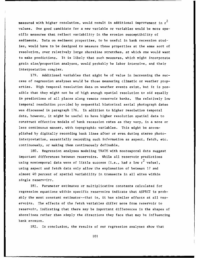
2
measured with higher resolution, would result in additional improvement in r
values. One good candidate for a new variable or variables would be more spe-
cific measures that reflect variability in the erosion susceptibility of
sediments. Data on sediment properties, to be useful in bank recession stud-
ies, would have to be designed to measure these properties at the same sort of
resolution, over relatively large shoreline stretches, at which one would want
to make predictions. It is likely that such measures, which might incorporate
grain size/proportion analyses, would probably be labor intensive, and their
interpretation complex.
179. Additional variables that might be of value in increasing the suc-
cess of regression analyses would be those measuring climatic or weather prop-
erties. High temporal resolution data on weather events exist, but it is pos-
sible that they might not be of high enough spatial resolution to aid equally
in predictions of all places along remote reservoir banks. The relatively low
temporal resolution provided by sequential historical aerial photograph dates
was discussed in paragraph 176. In addition to higher resolution temporal
data, however, it might be useful to have higher resolution spatial data to
construct effective models of bank recession rates as they vary, in a more or
less continuous manner, with topographic variables. This might be accom-
plished by digitally recording bank lines after or even during stereo photo-
interpretation, essentially recording such information as aspect, fetch, etc.
continuously, or making them continuously definable.
180. Regression analyses modeling TRATE with nontemporal data suggest
important differences between reservoirs. While all reservoir predictions2
using nontemporal data were of little success (i.e., had a low r value),
using aspect and fetch data only allow the explanation of between 17 and
almost 40 percent of spatial variability in transects in all sites within
single reservnirF.
181. Parameter estimates or multiplicative constants calculated for
regression equations within specific reservoirs indicate that ASPECT is prob-
ably the most constant estimator--that is, it has similar effects at all res-
ervoirs. The effects of the fetch variables differ more from reservoir to
reservoir, indicating that there may be important differences in the shapes of
shorelines rather than simply the directions they face that may be influencing
bank erosion.
182. In conclusion, the results of our regression analyses show that
101
bank recession rates are to some extent at least predictable through reference
to physically measurable, independent variables. The independent variables we
have used in this exploratory study are, however, not completely sufficient or
refined to allow more than about one-half of the variability in bank erosion
to be explained through regression analysis.
183. Probably the best way to actually predict the position of an
eroding reservoir bank at some time in the future, then, is to assume that
these same bank recession rates will continue with the same amount of varia-
tion in the foreseeable future. The new position of the bank at some time in
the future, then, can be expressed (after Dolan, Hayden, and Heywood 1978) by
an increments to the present shore position determined by
dS = dT [(rate of change) + k(standard deviation))
where S is the landward limit of the shore for a given time interval dT, and k
is the number of standard deviations required to give a desired probability
level. Then one would use additional information gained through these explor-
atory analyses to qualify or adjust predictions empirically arrived at.
Site Specific Measurements Using Electronic Image Analysis
184. The measurement technique focusing on transects spaced 100 m apart
along 2 km segments of the reservoir shore centered on the study site was de-
signed to allow the characterization of bank erosion trends through time at a
relatively wide range of spatial scales. The "philosophy" behind this method
is that bank recession at an archeological site is a process inherent in a
larger and more inclusive system, some of the components of which are sedi-
ments, the resezvcir pool with its wave and current dynamics, and the bank and
beach that form the interface between these components. This system operates
not simply at a specific spot along the shore, but is influenced by variabil-
ity in processes along a segment of shoreline. There is some question in the
literature on shoreline erosion (Phillips 1986) about just how great a reach
of shore must be considered to understand the operation of this system;
depending on the specific erosion related phenomena being studied, Phillips
recommends distances between 100 m and 60 km.
102

185. To more closely depict the effects of bank erosion on the actual
sites themselves, however, experiments were also undertaken using an alterna-
tive, and far more site specific, method. This method involves using enlarged
and electronically enhanced portions of aerial photographs, rather than
stereoscopic viewing. Even very large archeological sites are quite small in
most aerial photographs; a site measuring 500 m, for instance, appears only
2.5 cm across at a 1:20,000 scale. Interpretive overlay mapping of extremely
small areas leads to error which can constitute a large proportion of the
total measurements. Photographic enlargement, however, can lead to a degrada-
tion of resolution and contrast due to the creation of two new generations--a
negative and a positive--in the enlargement itself. If original photo scale
is sufficiently large, then photo enlargements are acceptable (Figure 16).
However, smaller-scale photographs such as that shown in Figure 17, at about
the same degree of enlargement as Figure 16, are more difficult to photo-
enlarge acceptably.
186. Electronic image enlargement and edge enhancement performed on an
International Imaging Systems analog image analysis system (Figure 18) were
employed in an attempt to remedy these problems. This system focuses a highly
Figure 16. Site 39LM224, 26 Oct 1938
103

INV*
Figure 17. Site 39LM224, 10 Oct 1984
Figure 18. Electronlc Image analysis system used to edge and contrastenhance magnified portions of aerial photographs for site-specific
mapping purposes
104

stable video camera equipped with a macro lens (and, if necessary, extension
rings and bellows) on - small portion of a photo placed on a light table. The
resulting video signal, without the multigenerational characteristics of suc-
cessive photo negatives and prints, is then processed. Contrast is increased
through a histogram stretch and edge enhancement. This procedure involves
superimposing otherwise identical negative and positive video signals and then
slightly delaying one signal to increase the definition of edges where photo
densities change. Edge enhancement is particularly effective on subtle linear
features--such as bank lines.
187. Successive aerial photographs showing three of the study sites,
39C06, 39LM224, and 39DW234, through time were analyzed using the analog image
analysis system, and slides were taken from the edge enhancer screen. A time-
series of these images depicting the Cable Site, 39LM224, in Lyman County,
South Dakota, is shown in Figures 19 through 26.
188. Next, the slides of the video images were projected, to scales of
about 1:1,000, and control points in and around the sites were used to ensure
rectification relative to one another. While details from the USGS quad
Figure 19. Site 39LM224, 26 Oct 1938
105

Figure 20. Site 39LM224, 1 Sep 1955
Figure 21. Site 39LM224, 21 Jun 1965
106

Figure 22. Site 39LM224, 23 Jul 1969
Figure 23. Site 39LM224, 15 May 1975
107

44
4-4!
Figure 24. Site 39LM224, 9 Apr 1977
Figure 25. Site 39LM224, 30 Oct 1981
108

Figure 26. Site 39LM224, 30 Oct 1984
sheets allowed the initial two-dimensional rectification of baseline site area
details, there was in some occasions insufficient map detail in the specific
site areas to allow the control of successive projections. For this reason
ephemeral control points, such as bushes or cultural features--visible from
one date to another, but not necessarily throughout the entire series--were
also used.
189. Maps for sites 39LM224, 39C06, and 39DW234 made in this manner,
including selected shoreline positions through time, are shown in Figures 27
through 29.
190. A digital planimeter was used to measure the areas of the sites as
they were prior to reservoir filling, and the successive amounts of site area
lost due to bank recession at later dates (Figure 30). It should be mentioned
here that defining the boundaries of a site is, in almost all cases, a rather
arbitrary exercise, whether it is done using evidence visible on aerial photo-
graphs or through survey or excavation on the ground. In the three experimen-
tal cases illustrated here, site boundaries were defined on the basis of cul-
tural features that could be cumulatively photointerpreted from the aerial
photographs--the maximum extent of fortification ditches and housepits, for
109

"to'/15/75
7/23169
Lyman County, South DakotaAPPROXIMATE SCALE'"s
0 no "0 MUI
Figure 27. Image analysis--derived site area map of the Cable Site, 39LM224
3- 2 ~
Corson County, South DakotaAPPROXIMATE SCALEas ON NoU@
Figure 28. Image analysis--derived site area map of theJake White Bull Site, 39C06
110

olk SITE !jo
A0A
-~s ~%\- -
81U241081 927/96
Dewey County, South DakotaAPPROXIMATE SCALE0 x" ac our?
Figure 29. Image analysis--derived site area map of the Moistad Site, 39DW234
Figure 30. Measurement of areas of sites lost using aNumonics digital planimeter

the most part. While these boundaries are not necessarily true in any sense,
they are consistent for within-site measurements.
191. Site area was plotted against aerial photograph dates for each
site (Figure 31), and regression equations derived for the resulting point
s0-
a0 39LM224
* 39DW234 0
0 o 39COO20
206 . . . .70 .. .75"'0"8
Photo Date
Figure 31. Graph of extinction curves for Sites 39DW234,
39C06, and 39LM224
swarms. It is interesting to note that the regression lines shown in this
figure are linear, and they fit their respective point swarms well. In dis-
cussions with field personnel at reservoirs, and in a majority of the more
theoretical literature, a recurrent theme is that while reservoir bank erosion
may be very rapid shortly after pool filling, a leveling off of erosion rates
should be noted soon due to the shoreline reaching an equilibrium state. In
support of this idea, it has been noted (Mollard 1986) that bank recession
proceeds much more slowly at natural lakes than at reservoirs of comparable
size in the same areas.
192. Unfortunately, no sign of the approach of such an equilibrium
state is given by the linear form of the regression lines in Figure 31. At
the only site to show a definite trend, as a matter of fact (39C06), the rate
of area loss may actually be increasing. Similar findings were announced by
Millsop (1985) as one result of high-resolution, on-the-ground measurements of
bank recession at Lake Sakakawea. There is no way to tell whether the absence
of diminishing bank erosion rates indicates that these rates will always re-
main high or whether the banks being studied here have simply not begun to
112

reach equilibrium in the 25 to 36 years that have elapsed since the closing of
the reservoirs.
193. As a final step in this exercise, the regression lines for each
site were projected to their intercept with the x axis, at which time--given a
linear area loss model--each site would theoretically be gone, or extinct. It
must be remembered, of course, that the boundaries used to measure initial
site areas were defined solely on the basis of photointerpretations of cul-
tural features. Given the large variations in erosion rates calculated much
more consistently and precisely along the 2 km shore reaches, there is no rea-
son tc believe that these "predictions" would necessarily be highly accurate,
certainly not to the extent implied by listing the day of extinction. We do
intend to be at those sites on their extinction days, however, to test these
predictions.
194. There are unavoidable geometric variations in images reproduced
from video screens, as well, which may affect the accuracy of maps compiled
from such images, although these probably constitute only a small error in
proportion to the enlarged size of the archeological sites in these rendi-
tions. We do feel, however, that the enlarged and enhanced views of immediate
site areas shown in the examples above, the site area maps, and the site
extinction dates given in Table 21 serve to dramatize in a graphic way the
impact of reservoir bank recession at these sites.
Table 21
Extinction Dates Predicted by
Regression Equations
Site Extinction Date
39LM224 I Mar 1994
39DW234 24 May 2019
39C06 8 Apr 2009
Conclusions and Recommendations
195. The research described here focuses on the detection, measurement,
and exploration of trends in, and causes of, bank erosion at archeolcgical
sites along the Middle Missouri River. The discussion of a few more specific
113

question areas addressed during the course of this research serves as a con-
clusion to this report. The discussion of these questions also suggests areas
in which additional, immediate, and longer-term activities and research might
be planned.
a. Is bank erosion causing impacts to archeological sites alongthe Middle Missouri River?
(1) In a specific sense, the results of this study illustrateconclusively that bank erosion is taking place at the12 sites studied. This erosion falls within the range ofgeneral reservoir bank erosion rates measured by physicalscientists in a number of similar studies. The amount oferosion also agrees with estimates given by archeologistsfor sites along Middle Missouri and other reservoirs.
(2) Although bank erosion is demonstrably taking place at allof the study sites, its rates are variable from site tosite. Determining the amount of management concern thatshould result from different rates of bank erosion ateach site will undoubtedly involve a complex equation inwhich many variables, including archeological signifi-cance and tradeoffs between economic and other resourcevalues, must figure. Exploration of such decision makingis beyond the scope of this study.
(3) Nonetheless, the results of this study emphasize thatthere is a pressing need to make such decisions. Some ofthe archeological sites studied will be gone within a fewdecades, as will probably hundreds more not studied. Itshould also be borne in mind that while archeologicalsites occupy only a small portion of the shores of Corpsof Engineers reservoirs, bank erosion is taking placealong entire shorelines where it threatens other re-sources such as vegetation, habitat, and the boundariesbetween public versus private property. Bank erosion isfar more than simply an archeological problem.
(4) Data such as those collected here, from historical andsequential aerial photographs, can serve as one of themajor bases for locating areas with differential rates ofbank erosion and for planning and prioritizing to meetthe problems posed by bank recession.
b. Can these effects be detected and measured using sequential,historical aerial photographs?
(1) The results of this study demonstrate that they can bedetected and measures via aerial photography. They alsosuggest that it is important to use as complete an aerialphotographic database as possible--that is, to discoverand use as many sets of aerial photographs as can befound--to ensure the maximum possible temporal resolutionand separate it from high resolution spatial variation.
14

(2) One of the major differences between this study and pre-vious bank erosion studies is the use of all available,appropriately scaled aerial photographs, rather than onlya few, to measure changes in bank position at each studysite.
(3) Even when all of the historical aerial photographs avail-able for an area through time are used, the temporalrepresentation of changes in bank position is not idealbut is variable through time. Using as large a selectionof aerial overflight dates as possible can help mitigatethis problem. Future bank erosion measurement effortsshould, for this reason, not attempt to use any sort ofsample of available, historical aerial photographs.
c. Can bank recession measurements from sequential, historicalaerial photographs serve as a data source for the estimationor prediction of future bank recession-related impacts toarcheological sites along the Middle Missouri Riverreservoirs?
(1) This question requires the consideration and separationof two types or dimensions of variation that can bestudied and predicted: temporal and spatial.
(2) Existing aerial photographs (not taken to measure banklines, but at the same time are all we have with which tomeasure), were taken at fortuitously variable times.They record the position of reservoir banks, of course,at the instants they were taken. As suggested by thebody of literature reviewed in this report, however, thedynamics of reservoir bank recession are caused by natu-ral or other factors of short duration, many of whichmight even be thought of as catastrophic. The incongru-ence of natural and photographic events, as well as thetemporal scale of their occurrences, make it likely thatwe will never be able to correlate time-specific inde-pendent variables with bank recession in a reliable way.
(3) If the purpose of doing so is to predict future bankrecession, one also would have to be able to predict thespecifics of future independent variables (storms andtheir intensity and location, for instance). Until thisis possible, predictions of concomitant bank recessionwill only be possible after the fact, in a high resolu-tion, temporal sense.
(4) A far more likely--and, upon contemplation, useful--prospect is the prediction of spatial variation in bankerosion at lower temporal scale. In the course of thisstudy, it was observed that bank recession rates arevariable over a range of spatial scales. While rateswere demonstrated to be variable between the study sites,they were in some cases much more variable within thesites.
115

(5) Variability at different spatial scales may be an ex-tremely important property of bank erosional dynamics fora number of reasons. First, the resources threatened bybank erosion are not constant over space but also havecharacteristic frequencies in different places. Forexample, archeological sites have been argued to bespaced not randomly but regularly in any number of argu-ments supported theoretically as well as with recourse todata. Spatial variation in the susceptibility of reser-voir banks to erosion, conditioned by nonrandom topo-graphic, pedological, and other properties at a range ofscales, must certainly be important in designing andengineering of physical bank protection measures, aswe11.
(6) If predictions could be made about bank recessionspecifying that while 95 percent of the bank in an areaof concern had to be protected (or its archeologicalrecord studied) and another 5 percent of the bank didnot, millions of dollars could be saved in only a fewmiles of shoreline.
(7) The results of this study suggest that it may be possibleto make such statements, at spatial frequencies between100 m and 1 km. It is likely that much higher and lowerspatial frequencies may also be important, however, inboth research and more practical terms. For this reason,future bank recession research should be designed toallow the collection of data with which the widest possi-ble range if spatial frequencies--from a few metresthrough entire reservoir bank lines--can be analyzed.
(8) The best way to collect such data would be to digitizeinterpretations of bank position at high resolution overentire reservoir bank lines. Such a data base wouldallow the application of power spectrum, Fourier, orother spatial analyses to investigate variability overtime at a wide range of spatial scales.
(9) Such analyses wuuld also ideally incorporate data onindependent variables such as archeological sites andmaterials, topographic variation, and other relevantnatural or cultural properties affecting bank erosionsusceptibility, also at a wide range of scales.
d. How consistent are bank recession rates at specificreservoirs, and how well can they be extended to otherreservoir bank recession rates?
(1) It is important to distinguish between spatial versustemporal variation in answering this question, as well.At a very general spatial scale, bank erosion at differ-ent places along reservoir shores is quite consistent,other things being equal. These other things can vary ata large scale, too, however. For instance, shore orien-tation, as compared to prevailing winds, causes bank
116

recession at even a gross spatial scale to be differenton opposite sides of a reservoir.
(2) At higher spatial scales, however, site-specific as wellas within-site characteristics are important. For thisreason, prospects for transferring some sort of generalpredictive model developed at specific places on onereservoir to specific places on another reservoir are notencouraging. Such a lack of high spatial resolution con-gruence, both within and between reservoirs, was probablyresponsible for Gatto and Doe's (1983) lack of success incorrelating bank recession at a large number of northernreservoirs (measured from aerial photographs) with allother assumed independent variables.
(3) One general observation about bank erosion and retreatthat can, however, be made on the basis of this study--and that crosses reservoir boundaries--is that bank ero-sion may be a more significant threat to archeologicalsites and materials (as well as to other bank properties,including encroachment into private land) than has beenimagined previously. The scientific literature on bankerosion, as well as experiential observations made bymany reservoir personnel, suggests the common senseprinciple that while reservoir banks would be expected toerode rapidly after reservoir filling, rates should slowor level off quickly. The results of this study illus-trate that this is not the case, at least at the sitesstudied here over a period of as much as 30 years. Bankerosion and recession may continue to be a relativelyconstant threat to the integrity of reservoir shorelinesand the resources they contain over long periods of time.
e. How can methods be improved in future studies of reservoirbank recession relevant to cultural resource studies, as wellas other bank recession measurements?
(1) Embodied in the previous conclusions are a number of sug-gestions. These suggestions concern data collection, howanalyses can be performed, and studies otherwise struc-tured, to enhance the value of future reservoir bank ero-sion studies and the usefulness of their results in prac-tical applications.
(2) First, more rather than fewer sets of aerial photographsshould be used to ensure the highest possible temporaldata resolution, thus possibly improving prospects ofpredicting erosion trends through time. Going hand-in-hand with the need for high temporal resolution bankretreat measurements is the necessity for collecting allrelevant independent data with a temporal dimension atscales which allow comparisons to be made with bankretreat data itself. Methods need to be devised, forinstance, to reduce such information as the characteris-tics of the weather, or of pool level fluctuations, to
117

measures that can be correlated with changes in bankposition through the variable time periods measurablefrom aerial photographs taken at fortuitous times in thepast.
(3) The widest possible range of spatial scales of bankretreat must also be available for future studies. Thiswill probably best be accomplished through the high-resolution digitization of the banklines across entirereservoir shores.
(4) A further argument for the measurement of the position ofbanks for entire reservoirs, and perhaps for all reser-voirs, is that reservoir shores and banks are logically amajor focus of Corps of Engineers interests and responsi-bilities. Reservoir shores and banks, in effect, are inand of themselves an important resource within the con-text of the Corps' responsibilities. Not knowing exactlywhere actively changing banklines of reservoirs are iscomparable to an agency such as the Park Service notknowing where their park boundaries are, or the Bureau ofLand Management not mapping the changing distribution ofrange resources.
(5) Measurements from aerial photographs, as illustrated bythis study, offer the best way to map both the positionsof past banklines, the locations of banklines in thepresent, and those of the future.
118

REFERENCES
Ahler, Stanley A., Davies, D. K., Falk, Carl R., and Madsen, D. B. 1974."Holocene Stratigraphy and Archeology in the Middle Missouri River Trench,South Dakota," Science, Vol 39, pp 905-908.
Abler, Stanley A., Cvancara, Alan M., Madsen, David B., and Kornbrath,Richard W. 1977. "Archeological Reconnaissance and Test Excavation at theTravis 2 Site, 39WW15, Oahe Reservoir, South Dakota," University of NorthDakota, Grand Forks; report submitted to the US Army Engineer District, Omaha,Omaha, NE.
Anderson, James R., Hardy, Ernest E., and Roach, John T. 1972. "A Land-UseClassification System for Use with Remote Sensor Data," US Geological SurveyCircular 671, US Geological Survey, Washington, DC.
Anderson, James R., Hardy, Ernest E., Roach, John T., and Witner, Richard E.1976. "A Land-Use and Land Cover Classification System for Use with RemoteSensor Data," Professional Paper 964, US Geological Survey, Washington, DC.
Blakeslee, Donald J., and O'Shea, John. 1983. "The Gorge of the Missouri:An Archeological Survey of Lewis and Clark Lake, Nebraska and South Dakota,"Wichita State University, Wichita, KS, report prepared for the US ArmyEngineer District, Omaha, Omaha, NE.
Brown, William M, Ill, Hines, Walter G., Rickert, David A., and Beach, Gary L.1979. "A Synoptic Approach for Analyzing Erosion as a Guide to Land-Use Plan-ning," Circular 715-L, US Geological Survey, Arlington, VA.
Bruun, Per, and Schwartz, Maurice L. 1985. "Analytical Predictions of BeachProfile Change in Response to a Sea Level Rise," Annals of Geomorphology, Sup-plementband 57, pp 34-50, Gerbuder Borntrager, Berlin.
Caldwell, W. W., and Henning, D. R. 1978. "North American Plains," Chronol-ogies in New World Archeology, R. E. Taylor and C. W. Meighan, eds.,Academic Press, New York, pp 113-245.
Carter, Charles H., and Guy, Donald E., Jr. 1983. "Lake Erie Shore Erosion,Ashtabula County, Ohio: Setting, Processes, and Recession Rates from 1876 to1973," Report of Investigations No. 122, Department of the Natural Resources,Division of Geological Survey, Columbus, OH.
Civco, Daniel L., Kennard, William C., and Lefor, Michael W. 1986. "Changesin Connecticut Salt-Marsh Vegetation as Revealed by Historical Aerial Photo-graphs and Computer-Assisted Cartographics," Environmental Management, Vol 10,No. 2, pp 229-239.
Clayton, Lee, Moran, S. R., and Bickley, W. E., Jr. 1976. "Stratigraphy,Origin and Climatic Implications of Late Quaternary Upland Silt in NorthDakota," Miscellaneous Series 54, pp 1-15, North Dakota Geological Survey.
Coogan, Alan H. 1987. "Holocene Geomorphic and Stratigraphic Framework ofArcheological Sites along the Missouri Pivar. Central SouLh Dakota," US ArmyEngineer District, Omaha, Omaha, NE.
Coogan, Alan H., and Irving, W. N. 1959. "Late Pleistocene and Recent Mis-souri River Terraces in the Big Bend Reservoir, South Dakota," Proceedings ofthe Iowa Academy of Sciences, Vol 66, pp 317-327.
119

Dean, R. G., and Maurer, E. M. 1984. "Models for Beach Profile Response,"CRC Handbook of Coastal Processes and Erosion, Paul D. Komar, pp 151-165.
Dietz, Robert S. 1963. "Wave-Base, Marine Profile of Equilibrium, and Wave-Built Terraces: A Critical Appraisal," Bulletin 74, pp 971-990, GeologicalSociety of America.
Dolan, Robert, and Hayden, Bruce. 1983. "Patterns and Prediction of Shore-line Change," CRC Handbook of Coastal Processes and Erosion, Paul D. Komar,ed., CRC Press, Inc., Boca Raton, FL.
Dolan, Robert, Hayden, Bruce, and Heywood, Jeffrey. 1978. "A New Photo-grammetric Method for Determining Shoreline Erosion," Coastal Engineering,Vol 2, pp 21-39.
Dolan, Robert, Hayden, Bruce P., May, Paul, and May, Suzette. 1980 (Oct)."The Reliability of Shoreline Change Measurements from Aerial Photographs,"Shore and Beach, pp 22-29.
Dolan, Robert, Hayden, Bruce, Rea, Cary, and Heywood, Jeffrey. 1979. "Shore-line Erosion Rates along the Middle Atlantic Coast of the United States,"Geology, Vol 7, pp 602-606.
Ebert, James I. 1982. "Photogrammetry: Tool for Documentation, Monitoringand Analysis of Cultural Resources," Technical Papers of the American Societyof Photogrammetry, ASP-ACSM Convention, March 14-20, 1982, Denver, CO,pp 57-61, American Society of Photogrammetry, Falls Church, VA.
• 1984. "Remote Sensing Applications in Archeology," Advances inArcheological Method and Theory, Vrl 7, Michael B. Schiffer, ed., AcademicPress, New York.
Ebert, James I., and Lyons, Thomas R. 1986. Measuring Archeological SiteErosion with Aerial Photographs, Interagency Archeological Services, NationalPark Service, San Francisco, CA.
Frison, George C. 1974. The Casper Site: A Hell Gap Bison Kill on the HighPlains, Academic Press, New York.
• 1976. "Cultural Activity Associated with Prehistoric MammothButchering and Processing," Science, Vol 194, pp 728-730.
. 1978. Prehistoric Hunters of the High Plains, Academic Press,New York.
Frison, George C., and Bradley, Bruce A. 1980. "Folsom Tools and Technologyat the Hanson Site, Wyoming," University of New Mexico Press, Albuquerque, NM.
Frison, George C., Walker, Danny N., Webb, Daviu S., and Zeimens, George M.1978. "Paleo-Indian Procurement of Camleops on the Northwestern Plains,"Quaternary Research, Vol 10, No. 3, pp 385-400.
Gatto, Lawrence W. 1982a. "Shoreline Conditions and Bank Recession Along theU.S. Shorelines of the St. Marys, St. Clair, Detroit and St. Lawrence Rivers,"Report 82-11, US Army Cold Regions Research and Engineering Laboratory,Hanover, NH.
• 1982b. "Reservoir Bank Erosion Caused and Influenced by IceCover," Special Report 82-31, US Army Cold Regions Research Engineering Labor-atory, Hanover, NH.
120

Gatto, Lawrence W. 1984a. "Informal Memorandum: Technical Note: ReservoirBank Erosion Measurement Techniques," US Army Cold Regions Research andEngineering Laboratory, Hanover, NH.
. 1984b. "Tanana River Monitoring and Research Program: Rela-tionships Among Bank Recession, Vegetation, Soils, Sediments and Permafrost onthe Tanana River Near Fairbanks, Alaska," Special Report 84-21, US Army ColdRegions Research and Engineering Laboratory, Hanover, NH.
. 1984c. "Reservoir Bank Erosion Caused by Ice," Cold RegionsScience and Technology, Vol 9, pp 203-214.
• 1988. "Techniques for Measuring Reservoir Bank Erosion," SpecialReport 88-3, US Army Cold Regions Research and Engineering Laboratory,Hanover, NH.
Gatto, Lawrence W., and Doe, William W., III. 1983. "Historical Bank Reces-sion at Selected Sites Along Corps of Engineers Reservoirs," SpecialReport 83-30, US Army Cold Regions Research and Engineering Laboratory,Hanover, NH.
• 1987. "Bank Conditions and Erosion Along Selected Reservoirs,"Environmental Geology and Water Sciences, Vol 9, No. 3, pp 143-154.
Gilbert, G. K. 1884. "The Topographic Features of Lake Shores," Report ofthe Director of the US Geological Survey, Vol 5, pp 75-123, US Geological Sur-vey, Washington, DC.
Haug, James K. 1976. "Archeological Survey of Coldbrook and CottonwoodSprings Reservoirs, Fall River County, South Dakota," US Army Engineer Dis-trict, Omaha, Omaha, NE.
Huddleston, T. E. 1948. "Random Notes on Aerial Photography as Applied toPlains Archeology," Plains Archeological Conference Newsletter, Vol 1, No. 3,pp 5-7.
ITEK Corporation. 1965a. "Archeological Photointerpretations of the Brule-Crow Creek Indian Reservation Area, South Dakota," Manuscript on file at theMidwest Archeological Center, National Park Service, Lincoln, NE.
• 1965b. "Archeological Photointerpretation," Manuscript on fileat the Midwest Archeoligical Center, National Park Service, Lincoln, NE.
Johnson, A. E. 1976. "Hopewellian Archeology in the Lower Missouri Valley,"Publications in Anthropology No. 8, University of Kansas, Lawrence, KS.
Lawson, Daniel E. 1985. "Erosion of Northern Reservoir Shores," Mono-graph 85-1, US Army Cold Regions Research Engineering Laboratory, Hanover, NH.
Lehmer, Donald J. 1971. "Introduction to Middle Missouri Archeology," Na-tional Park Service, US Department of the Interior, Washington, DC.
Loelkes, George L., Jr., Howard, Gordon E., Jr., Schwertz, Eddie L., Jr.,Lampert, Phillip D., and Miller, Stephan W. 1983. "Land Use/Land Cover andEnvironmental Photointerpretation Keys," Bulletin 1600, US Geological Survey,Alexandria, VA.
121
Lyons, Thomas R., and Ebert, James 1. 1982. "Photogrammetric Measurement andMonitoring of Historic and Prehistoric Structures," Conservation of HistoricStone Buildings, pp 242-271, Report of the Committee on Conservation of His-toric Stone Buildings and Monuments, National Research Council, Washington,DC, National Academy Press.
Millsop, Mark D. 1985. A Quantitative Analysis of Shoreline Erosion Pro-cesses, Lake Sakakawea, North Dakota, M.A. Thesis, Department of Geology,University of South Dakota, Grand Forks, SD.
Mollard, J. D. 1986 (May). "Shoreline Erosion and Slumping Studies onPrairie Lakes and Reservoirs," Paper presented at Symposium on CohesiveShores, National Research Council Associates Committee for Research on Shore-line Erosion and Sedimentation, Burlington, Ontario, Canada.
Neuman, Robert W. 1975. "The Sonata Complex and Associated Sites on theNorthern Great Plains," Publications in Anthropology No. 6, Nebraska StateHistorical Society.
Nowak, Timothy R., Hannus, L. Adrien, and Lueck, Edward J. 1982. "A Pre-historic and Historic Overview of Northeastern South Dakota," Cultural Re-source Investigations of the South Dakota Segment of the Northern BorderPipeline, Peter Winham, Katherine Winham, Edward Lueck, Lynette Rossum, andJohn Butterbrodt, eds., Vol 4, pp 25.1-25.74, South Dakota State UniversityArcheology Laboratory, Brookings, SD.
Phillips, Jonathan D. 1986. "Spatial Analysis of Shoreline Erosion, DelawareBay, New Jersey," Annals of the Association of American Geographers, Vol 76,No. 1, pp 50-62.
Ray, Richard G. 1960. "Aerial Photographs in Geologic Interpretation andMapping," Professional Paper No. 373, US Geological Survey, Washington, DC.
Reeves, Brian 0. K. 1973. "The Concept of an Altithermal Cultural Hiatus inNorthern Plains Prehistory," American Anthropologist, Vol 75, No. 5,pp 1221-1253.
Reid, John R., Jr. 1985. "Bank-erosion Processes in a Cool-temperate Envi-ronment, Orwell Lake, Minnesota," Geological Society of America Bulletin,Vol 96, pp 781-792.
Riley, D. N. 1987. Air Photography and Archeology, Duckworth, London.
Sanders, Paul H., Penny, Dori M., McFaul, Michael L., Dueholm, Keith H.,Schwiegert, Kurt P., and Larson, Thomas K. 1987. "A Cultural Resource In-ventory of Portions of Lake Oahe, Corson County, South Dakota," Vol I, Reportprepared for the US Army Engineer District, Omaha, Omaha, NE, by Larson-Tibesar, Laramie, WY.
SAS Institute, Inc. j985. SAS-STAT Guide for Personal Computers, 6th ed,Cary, NC.
Shabica, Stephen V., Dolan, Robert, May, Suzette, and May, Paul. 1984."Shoreline Erosion Rates Along Barrier Islands of the North Central Gulf ofMexico," Environmental Geology, Vol 5, No. 3, pp 115-126.
Slama, Chester C. 1980. "Manual of Photogrammetry," American Society ofPhotogrammetry, Falls Church, VA.
122

Slizeski, Joseph J., Andersen, John L., and Dorough, Wayne G. 1982. "Hydro-logic Setting, System Operation, Present and Future Stresses," The MissouriRiver Study Group, L. W. Hesse, ed., pp 14-37.
Solecki, Ralph S. 1952 (Sep). "Photographing the Past," Missouri BasinProgress Report, pp 42-48, US Department of the Interior, Interior MissouriBasin Field Committee, Billings, MT.
. 1957. "Practical Aerial Photography for Archeologists," AmericanAntiquity, Vol 22, No. 4, pp 337-351.
Steinacher, Terry L. 1983. "Archeological Investigations at the WhistlingElk Site (39HU242), 1978-1979," Archeological Investigations Within FederalLands Located on the East Bank of the Lake Sharpe Project Area, South Dakota:1978-1979, Final Report, Technical Report 83-04, Vol II, Appendix I, Sec-tion A, University of Nebraska-Lincoln, Division of Archeological Research,Lincoln, NE; report prepared for the US Army Engineer District, Omaha, Omaha,NE.
Strandberg, C. H. 1967. "Photoarcheology," Photogrammetric Engineering,Vol 33, No. 10, pp 1152-1157.
Stubbs, Stanley A. 1950. "Bird's Eye View of the Pueblos," University ofOklahoma Press, Norman, OK.
Tanner, W. F. 1978. "Standards for Measuring Shoreline Change," Report ofthe Ad Hoc Committee Workshop, Coastal Research and Department of Geology,Florida State University, Tallahassee, FL.
Toom, Dennis L., and Picha, Paul R. 1984. "An Archeological Survey of Se-lected Federal Lands on the West Bank of the Big Bend/Lake Sharpe ProjectArea, Lyman and Stanley Counties, South Dakota, 1983; Main Report," Contribu-tion No. 198, Department of Anthropology and Archaeology, University of NorthDakota, Grand Forks, ND; report prepared for US Army Engineer District, Omaha,Omaha, NE.
US Army Engineer Division, Missouri River. 1986. "1986-1987 Missouri RiverMain Stem Reservoirs Annual Operating Plan and Summary of Actual 1985-1986Operations," Missouri River Reservoir Control Center, Omaha, NE.
Warren, Robert E. 1987. "The Impact of Bank Erosion on Prehistoric CulturalResources in the Lower Illinois River Valley," Technical Report 87-211-10,Illinois State Museum Society, Quaternary Studies Program, Springfield, TL.
Wedel, Waldo R. 1961. "Prehistoric Man on the Great Plains," University ofOklahoma Press, Norman, OK.
• 1978. "The Prehistoric Great Plains," Ancient Native Americans,Jesse D. Jennings, ed., W. H. Freeman, San Francisco, CA, pp 182-219.
Weston, Timothy, Goulding, Douglas, and Ahler, Stanley A. 1979. "Archeologi-cal Monitoring and Shoreline Reconnaissance at the Travis 2 Site, 39WW15, OaheReservoir, South Dakota," University of North Dakota, Grand Forks, ND; reportprepared for the US Army Engineer District, Omaha, Omaha, NE.
Wettlaufer, Boyd. 1955. "The Mortlach Site in the Besant Valley of CentralSaskatchewan," Saskatchewan Museum of Natural History, Regina, Canada.
123

Wheat, Joe Ben. 1972. "The Olsen-Chubbuck Site: A Paleo-lndian Bison Kill,"American Antiquity, Vol 37, No. 1, Plains Anthropology Society, Lincoln, NE.
. 1979. "The Jurgens Site," Plains Anthropologist Memoir 15,
Plains Anthropological Society, Lincoln, NE.
Wilmsen, Edwin N. 1974. Lindenmeier: A Pleistocene Hunting Society, Harperand Row, New York.
Wood, W. Raymond, Nickel, Robert K., and Griffin, David E. 1984. "RemoteSensing: The American Great Plains," Division of Cultural Resources, NationalPark Service, Washington, DC.
Zubrow, Ezra B. W. 1974. "Population, Contact, and Climate in the New Mexi-can Pueblos," Antropological Papers of the University of Arizona, Tucson, AZ.
124

APPENDIX A
AERIAL PHOTOGRAPHS COVERING MIDDLE MISSOURI RIVER STUDY SITES
(Data on file at US Army Engineer WaterwaysExperiment Station (WES) CEWES-EE-R)

APPENDIX B
BANK RECESSION MEASURES SITE TABLES AND GRAPHS
(Data on file at US Army Engineer WaterwaysExperiment Station (WES) CEWES-EE-R)