pastel.archives-ouvertes.fr · · 2018-02-23hal id: pastel-00666690 submitted on 6 feb 2012 hal...
TRANSCRIPT

HAL Id: pastel-00666690https://pastel.archives-ouvertes.fr/pastel-00666690
Submitted on 6 Feb 2012
HAL is a multi-disciplinary open accessarchive for the deposit and dissemination of sci-entific research documents, whether they are pub-lished or not. The documents may come fromteaching and research institutions in France orabroad, or from public or private research centers.
L’archive ouverte pluridisciplinaire HAL, estdestinée au dépôt et à la diffusion de documentsscientifiques de niveau recherche, publiés ou non,émanant des établissements d’enseignement et derecherche français ou étrangers, des laboratoirespublics ou privés.
Three-dimensional modeling of radiative and convectiveexchanges in the urban atmosphere
Yongfeng Qu
To cite this version:Yongfeng Qu. Three-dimensional modeling of radiative and convective exchanges in the urban at-mosphere. Earth Sciences. Université Paris-Est, 2011. English. <NNT : 2011PEST1111>. <pastel-00666690>
ÉCOLE DES PONTS PARISTECH / UNIVERSITÉ PARIS-EST
P H D T H E S I Sto obtain the title of
PhD of the Université of Paris-Est
Specialty : SCIENCE , ENGINEERING AND ENVIRONMENT
Defended by
Yongfeng QU
Three-dimensional modeling of radiative
and convective exchanges in the urban
atmosphereProvisional date of defense: November 18, 2011
Jury :
Reviewers : Dr. Majorie MUSY - CERMA
Dr. Valéry MASSON - Météo-France
Examinators : Pr. Jean François SINI - École Centrale de Nantes
Pr. Jean Philippe GASTELLU-ETCHEGORRY - CESBIO
Pr. Marina K.A. NEOPHYTOU - University of Cyprus
Dr. Patrice G. MESTAYER - IRSTV
Advisor : Dr. Bertrand CARISSIMO - CEREA
Co-advisor : Dr. Maya MILLIEZ - CEREA
Co-advisor : Dr. Luc MUSSON-GENON - CEREA

Acknowledgments
This research was conducted with the financial support from EDF. I thank Grégoire Pigeon for
providing access to the CAPITOUL data and the Defense ThreatReduction Agency (DTRA)
for providing access to the MUST data.
I would like to express my gratitude to my advisor, Bertrand Carissimo, for his insight-
ful suggestions and guidance. More particularly, I must thank my co-advisor, Maya Milliez,
whose endless patience, good-natured helpfulness, throughout kept the thesis on track and sub-
stantially improved it at every stage. I would like also to recognize the contribution of my
co-advisor Luc Musson-Genon who gave me invaluable advice and provided me administra-
tive assistance on numerous occasions.
I would like to express my sincere gratitude to Majorie Musy and Valéry Masson who take
precious time off from their tight schedule to be reviewer. Iam also greatly indebted to Jean-
François Sini, Jean Philippe Gastellu-Etchegorry, Patrice Mestayer and Marina Neophytou to
be the jury committee members.
My thanks go also to Christian Seigneur, Director of the CEREA, for hosting me in his
laboratory. Thanks to all the CEREA members who have instructed and helped me a lot in the
past three years. Also thanks to the personel of the university of Paris-Est and doctoral School
for their kind support.
I am also grateful to the department MFEE of EDF R&D for hosting me in Chatou and for
providing the facilities to conduct this thesis.
I would also like to acknowledge the CERMA laboratory for their technical assistance on
the SOLENE software, especially, Julien Bouyer and LaurentMalys.
I am greatly indebted to people for their many helpful suggestions and comments: Richard
Howard, Alexandre Douce, Namane Méchitoua, David Monfort,Patrice Mestayer, Majorie
Musy, James Voogt, Jörg Franke, Marina Neophytou, Bert Blocken, Dominique Groleau.
Special thanks go to my friends and colleges who have supported me throughout my re-
search: Denis Wendum, Dominique Demengel, Eric Gilbert, Eric Dupont, Raphael Bresson,

ii
Cédric Dall’ozzo, Fanny Coulon, Venkatesh Duraisamy, Marie Garo and Hanane Zaïdi and
many others.
There is not enough space, here, to mention all the people whohave helped me, with scien-
tific discussions, or with their friendship and encouragement, during this thesis work. I would
like to thank all of them.

Contents
1 Context and objectives 1
1.1 Background. . . . . . . . . . . . . . . . . . . . . . . . . . . . . . . . . . . . 1
1.1.1 Urban heat island. . . . . . . . . . . . . . . . . . . . . . . . . . . . . 2
1.1.2 Air quality . . . . . . . . . . . . . . . . . . . . . . . . . . . . . . . . 3
1.1.3 Energy management. . . . . . . . . . . . . . . . . . . . . . . . . . . 3
1.1.4 Pedestrian wind comfort. . . . . . . . . . . . . . . . . . . . . . . . . 4
1.2 Urban physics. . . . . . . . . . . . . . . . . . . . . . . . . . . . . . . . . . . 5
1.2.1 Spatial and temporal scales and urban boundary layer. . . . . . . . . . 5
1.2.2 Urban energy balance. . . . . . . . . . . . . . . . . . . . . . . . . . 8
1.3 Objectives and structure of the thesis. . . . . . . . . . . . . . . . . . . . . . . 12
2 Model design 15
2.1 General CFD modeling approach for the urban environment. . . . . . . . . . 15
2.1.1 Best practice guidelines. . . . . . . . . . . . . . . . . . . . . . . . . 18
2.1.2 Mesh issues. . . . . . . . . . . . . . . . . . . . . . . . . . . . . . . . 27
2.2 Review of some Urban Energy Balance Models. . . . . . . . . . . . . . . . . 32
2.2.1 Urban Energy Balance Modeling. . . . . . . . . . . . . . . . . . . . . 32
2.2.2 International Urban Energy Balance Models Comparison . . . . . . . . 35
2.3 A new coupled radiative-dynamic 3D scheme inCode_Saturne for modeling
urban areas . . . . . . . . . . . . . . . . . . . . . . . . . . . . . . . . . . . . 38
2.3.1 Presentation of the atmospheric module inCode_Saturne . . . . . . . . 39
2.3.2 3D Atmospheric Radiative model. . . . . . . . . . . . . . . . . . . . 42
2.3.3 Surface temperature models. . . . . . . . . . . . . . . . . . . . . . . 47
2.3.4 Convection model. . . . . . . . . . . . . . . . . . . . . . . . . . . . 50

iv Contents
3 Micrometeorological modeling of radiative and convective effects with a building
resolving code: published in Journal of Applied Meteorology and Climatology,
(2011) 50, 1713–1724 53
4 A comparison of two radiation models:Code_Saturne and SOLENE 67
4.1 Introduction. . . . . . . . . . . . . . . . . . . . . . . . . . . . . . . . . . . . 67
4.2 Description of SOLENE model. . . . . . . . . . . . . . . . . . . . . . . . . . 70
4.2.1 Geometry and mesh. . . . . . . . . . . . . . . . . . . . . . . . . . . 70
4.2.2 Thermo-radiative model. . . . . . . . . . . . . . . . . . . . . . . . . 72
4.3 Radiation analyses. . . . . . . . . . . . . . . . . . . . . . . . . . . . . . . . 74
4.3.1 Set-up for radiation computation. . . . . . . . . . . . . . . . . . . . . 74
4.3.2 Comparison of direct solar flux. . . . . . . . . . . . . . . . . . . . . . 75
4.3.3 Comparison of diffuse solar flux. . . . . . . . . . . . . . . . . . . . . 77
4.3.4 Comparison of long-wave radiation flux. . . . . . . . . . . . . . . . . 80
4.3.5 Comparison of surface temperatures. . . . . . . . . . . . . . . . . . . 81
4.4 Conclusions and perspectives. . . . . . . . . . . . . . . . . . . . . . . . . . . 82
5 Numerical study of the thermal effects of buildings on low-speed airflow taking
into account 3D atmospheric radiation in urban canopy: paper submitted to Jour-
nal of Wind Engineering & Industrial Aerodynamics 87
6 Validation with CAPITOUL field experiment 120
6.1 Introduction. . . . . . . . . . . . . . . . . . . . . . . . . . . . . . . . . . . . 121
6.2 Overview of CAPITOUL field experiment. . . . . . . . . . . . . . . . . . . . 121
6.2.1 Objectives and description of the site. . . . . . . . . . . . . . . . . . 122
6.3 Simulation set-up. . . . . . . . . . . . . . . . . . . . . . . . . . . . . . . . . 126
6.3.1 Choice of the computational domain. . . . . . . . . . . . . . . . . . . 127
6.3.2 Mesh strategy. . . . . . . . . . . . . . . . . . . . . . . . . . . . . . . 127
6.3.3 Initial and boundary conditions. . . . . . . . . . . . . . . . . . . . . 128

Contents v
6.4 Results and discussion. . . . . . . . . . . . . . . . . . . . . . . . . . . . . . 131
6.4.1 Comparison of IRT pictures. . . . . . . . . . . . . . . . . . . . . . . 131
6.4.2 Comparison of the local diurnal evolution of brightness surface tem-
peratureTbr . . . . . . . . . . . . . . . . . . . . . . . . . . . . . . . . 138
6.4.3 Model-Observation comparison of heat fluxes. . . . . . . . . . . . . . 139
6.4.4 Model-Observation comparison of friction velocityu∗ . . . . . . . . . 144
6.4.5 Statistical comparison with hand-held IRT data. . . . . . . . . . . . . 147
6.5 Conclusions and perspectives. . . . . . . . . . . . . . . . . . . . . . . . . . . 153
7 Conclusions and Future Work 155
7.1 Summary and Conclusions. . . . . . . . . . . . . . . . . . . . . . . . . . . . 155
7.2 Perspectives. . . . . . . . . . . . . . . . . . . . . . . . . . . . . . . . . . . . 158
Bibliography 161


CHAPTER 1
Context and objectives
Contents
1.1 Background . . . . . . . . . . . . . . . . . . . . . . . . . . . . . . . . . . . . 1
1.1.1 Urban heat island. . . . . . . . . . . . . . . . . . . . . . . . . . . . . . 2
1.1.2 Air quality . . . . . . . . . . . . . . . . . . . . . . . . . . . . . . . . . 3
1.1.3 Energy management. . . . . . . . . . . . . . . . . . . . . . . . . . . . 3
1.1.4 Pedestrian wind comfort. . . . . . . . . . . . . . . . . . . . . . . . . . 4
1.2 Urban physics . . . . . . . . . . . . . . . . . . . . . . . . . . . . . . . . . . . 5
1.2.1 Spatial and temporal scales and urban boundary layer. . . . . . . . . . . 5
1.2.2 Urban energy balance. . . . . . . . . . . . . . . . . . . . . . . . . . . 8
1.3 Objectives and structure of the thesis . . . . . . . . . . . . . . . . . . . . . . 12
1.1 Background
Urbanization is a sign of modernization, industrialization and mobilization. It implies for a
transformation in the social environment, political organization and division of work. On the
other hand, rapid urban extension in the last century had far-reaching consequences for sus-
tainability and had profoundly changed the environment by everyday activities. Furthermore,
more than half of the world’s population live in urban areas.As described byOke(1987), the
process of urbanization produces radical changes in the nature of the surface and atmospheric

2 Chapter 1. Context and objectives
properties of a region. It involves the transformation of the radiative, thermal, hydrology and
aerodynamic characteristics and thereby alters the natural energy and hydrology balances, as
well as the wind and turbulence levels.
Therefore, among the many issues and challenges involved inurban development, are the
environment ones, such as:
• Urban heat island
• Air quality
• Pedestrian wind comfort
• Energy management
1.1.1 Urban heat island
The Urban Heat Island (UHI) phenomenon consists in an increased air temperature within
cities in comparison to the rural surroundings. It was first identified byHoward(1820) over
the city of London. Especially at night, the air temperaturedifference can reach 3 to 10K
for large agglomerations (Oke, 1987). The deterioration of the urban thermal environment has
been recognized as a serious problem during the summer months even in mid-latitude regions.
During heat waves, it can lead to serious consequences in terms of public health. This was
revealed during a important heat wave in August 2003 that affected Europe and caused more
than 70, 000 victims, with a majority in urban areas (15, 000 in France) (Hémon and Jougla,
2003). This deterioration could become worse in the context of climate change (temperature
increase even larger in cities due to a positive feedback) (McCarthy et al., 2010).
Consequently, urban development initiatives that consider the influence on the urban ther-
mal environment have received more attention than they havein the past. In addition, a ther-
mally comfortable environment would be pleasant for the inhabitants and commuters in urban
areas.

1.1. Background 3
It is also worth noting that the UHI is seen during both summerand winter. Rational uti-
lization of the UHI effect in winter may get some advantages:reducing the need for heating,
making the snow on the roads melt faster etc. Moreover, most plants are sensitive to temper-
atures and only grow above a certain threshold. In areas which are affected by the UHI effect
there is more growth in most plants, so whilst it may be practical from an agricultural point of
view.
1.1.2 Air quality
The heat wave that struck Europe in summer 2003 was not only extreme in temperature but also
in the persistence of high ozone concentrations for almost three weeks. The World Health Or-
ganization (WHO) states that more than two million people die each year from causes directly
attributable to air pollution (WHO, 2006). Current research concludes that emissions in build-
ings are one of the major sources of the pollution that causesurban air quality problems, and
pollutants that contribute to climate change. They accountfor 49% of sulfur dioxide emissions,
25% of nitrous oxide emissions, and 10% of particulate emissions, all of which damage urban
air quality. From the source of World Resource Institute, based on data for 2000, buildings (in-
cluding residential and commercial buildings) produce 15.3% greenhouse gas emissions ahead
of industry (10.4%) and transportation (13.5%) sectors. In that event, sustainable develop-
ment requires the improvement of the interrelationships between a building, its components, its
surroundings, and its occupants.
1.1.3 Energy management
The World Business Council for Sustainable Development (WBCSD, 2009) points out that
40% of the world’s energy use is consumed in buildings. New buildings that will use more
energy than necessary are being built every day, and millions of today’s inefficient buildings
will remain in 2050. On one side, in order to reduce the globalenergy-related carbon footprint
by 77% or 48 Gigatons to stabilize CO2 levels in order to reach the ones recommended by

4 Chapter 1. Context and objectives
the Intergovernmental Panel on Climate Change (IPCC), the building sector must radically
make cut in energy consumption. On the other side, this presents an excellent opportunity for
business to develop new products and services that cost-effectively reduce the energy burden on
consumers and countries while contributing to the slowdownof climate change. This market
could be worth between US$ 0.9 trillion and US$ 1.3 trillion.
1.1.4 Pedestrian wind comfort
Near high-rise buildings, it can happen that wind reaches high velocities at pedestrian levels,
contributing to general discomfort of the city inhabitantsor even being dangerous. In March
2011, in the United Kingdom, high winds blustered in Yorkshire for almost one day long,
causing some minor structural damages to buildings and roads. Moreover, a report of the Daily
Mail described how a pedestrian was killed and another injured when a lorry overturned and
toppled over them during a high wind episode in the center of the city of Leeds. Actually,
there have already been recorded instances of people being blown off their feet near high-rise
buildings.Lawson and Penwarden(1975) reported dangerous wind conditions to be responsible
for the death of two old ladies in 1972 after being blown over by sudden wind gusts.
On the other hand, in weak wind region, the use of urban ventilation helps to decrease the
UHI intensity. This is definitely an advantage with the raising concerns regarding the cost and
environmental impact of energy use. Not only does wind provide natural ventilation (outdoor
air) to ensure safe healthy and comfortable conditions for building occupants without the use
of fans, it also provides free cooling without the use of mechanical systems. Adequate urban
ventilation is also helpful to reduce air pollutant dispersion around buildings (Shirasawa et al.,
2008).
In fact, the construction of a building inevitably changes the microclimate and the ventila-
tion in its vicinity. Therefore, the design of a building should not only focus on the building
appearance and on providing good indoor environment, but should also include the effect of its
architecture on the outdoor environment. The impact of buildings on outdoor environment, in

1.2. Urban physics 5
particular related to wind, has received relatively littleattention, so far.
1.2 Urban physics
As a consequence of these issues, focus was given on the research in the field of urban physics,
aiming to better understand and model the phenomena occurring in urban areas and the atmo-
sphere above, such as heat, moisture and momentum transfers, pollutant and acoustic disper-
sion, radiative transfer etc. Urban physics cover a large range of disciplines: meteorology, fluid
dynamics, thermal, aerodynamics, and acoustics etc. For instance, in the field of wind engi-
neering, urban physics analyze the effects of wind in the built-up environment and studies the
possible damages or benefits which may result from wind. In the fields of air pollution, urban
physics also includes low and moderate winds as these are relevant to dispersion of contami-
nants.
1.2.1 Spatial and temporal scales and urban boundary layer
The interactions between urban areas and the atmosphere above imply various scales.Orlanski
(1975) gives a rational subdivision of scales for atmospheric processes:
• synoptic scale (scale of largest cyclones, distance largerthan 2000km)
• mesoscale (between synoptic scale and larger than microscale, from 2000km to 200km
and from 200kmto 2km)
• microscale (near-ground atmospheric phenomena, distanceless than 2km). More re-
cently, microscale includes smaller scales, such as: building scale (less than 100m),
building component scale (less than 10m) even building material scale.
Scale dependent parameterizations are needed to include the influences of built-up areas
on meteorological fields in atmospheric models. In order to study to impact of an urban area
on its surroundings (scale varying from 10 to 100km) mesoscale modeling is used, where the

6 Chapter 1. Context and objectives
influence of obstacles is parameterized. In order to study the phenomena occurring within
the urban canopy (scale varying from 100m to 2km) obstacle resolving microscale models are
used, where the obstacles are explicitly included in the mesh. Nevertheless, while characteristic
scales of phenomena resulting from single obstacles are relatively small (∼ 100m, ∼ minutes)
and can be resolved, in reality there are always multiple obstacles as, for example in urban
areas; many buildings, in a wind turbine park; many turbines, or in a forest; many trees. In
these cases, hardly all obstacles can be resolved with sufficient detail, and their impacts need to
be parameterized (Schlünzen et al., 2011). To additionally calculate the interaction of canopy
layer processes and the air above, a coupling between mesoscale and microscale models can
be used. Based onOrlanski(1975) andRanderson(1976), Schlünzen et al.(2011) (Fig. 1.1)
summarize the spatial scales of phenomena that can be directly simulated in a mesoscale model
and microscale model and that have to be parameterized in a model or to be considered via the
boundary values. The boundary layer over an urban area is of particular interest as it is in this
layer of the atmosphere that the majority of observations inurban areas are made (Oke, 1987;
Stull, 1988). It is therefore important to know what these observationsrepresent. As air flows
from one surface to another an internal boundary layer forms. The internal boundary layer is
influenced by the new surface and deepens with fetch. The internal boundary layer formed over
urban areas is the urban boundary layer (UBL) (Oke et al., 1999; Stull, 1988). The buildings
introduce a large amount of vertical surfaces, high roughness elements, artificial materials, and
impervious surfaces (such as buildings and pavements that are made of dark colors absorb the
heat which causes the temperature of the surface and surrounding air to increase). The most
well-known consequences are the UHI, the generation of local flows between the city centre and
its outskirts and between the various city districts, and the "urban plume" downwind of a city.
In calm or low wind condition, the warmer air in the city core rises, pulling air near the surface
radically inward and a radially outward return flow develop aloft. This air circulation forms
the "urban dome"(a dome of heated air above the cities due to pressure differences between
warmer temperatures in the city and cooler temperatures in the surrounding rural areas). The

1.2. Urban physics 7
Figure 1.1: Spatial and temporal scales of atmospheric phenomena and how these phenomena
are treated in Reynolds-Averaged Navier-Stokes (RANS) mesoscale or obstacle resolving mi-
cro scale models (right columns). Dashed areas in the right columns indicate the currently used
RANS model resolutions and the resulting possibly resolvable minimum phenomena sizes.
FromSchlünzen et al.(2011).

8 Chapter 1. Context and objectives
UBL structure and its various sub-layers are depicted in Figure1.2.
Figure 1.2: Schematics of the urban boundary-layer structure indicating the various (sub)layers
and their names. a) PBL: planetary boundary layer; in b) UCL:urban canopy layer; in c) SVF:
sky view factor. FromRotach et al.(2005); modified afterOke(1987).
1.2.2 Urban energy balance
Knowledge of the surface energy balance is essential to understand urban climate and boundary
layer processes (Oke, 1987). Oke (1987) defines the energy balance for a building and air
volume containing the net radiationQ∗ (W m−2), the sensible heat fluxQH (W m−2), the
latent heat fluxQE (W m−2), storage∆QS (W m−2), the advective flux∆QA (W m−2), and the
anthropogenic heat fluxQF (W m−2) as illustrated in Figure1.3, with the following equilibrium

1.2. Urban physics 9
relationship:
Q∗ +QF = QH +QE +∆QS+∆QA, (1.1)
whereQ∗ (W m−2) is the net radiation flux through the top of the volume,QF (W m−2) is
the anthropogenic heat flux release within the volume,QH (W m−2) andQE (W m−2) refer to
convection of sensible heat flux and latent heat flux respectively through the top of the volume.
The terms∆QS (W m−2) and∆QA (W m−2) are storage of heat in the ground and the build-
ings and advective heat transfer within the volume. Note that here the terms "convection"and
"advection"refer to vertical turbulent transfer and mean horizontal transfer, respectively.
For dry surfaces, the energy balance in equation (1.1) is simplified by neglectingQE, and if
the sites are horizontally homogeneous,∆QA can be also ignored. Therefore, surface temper-
ature results from the balance of energy exchanges at the surface given the incoming radiative
forcing, the local ambient air temperature, and the surfaceradiative properties.
Figure 1.3: Schematics of the urban energy balance in an urban building-air volume. From
Oke (1987). The base of the averaging volume is determined as the levelacross which there
is negligible energy transfer on time scales of less than a day. With: Q∗ (W m−2) is the net
radiation;QH (W m−2) the sensible heat flux;QE (W m−2) the latent heat flux;∆QS (W m−2)
storage;∆QA (W m−2) the advective flux; andQF (W m−2) the anthropogenic heat flux.

10 Chapter 1. Context and objectives
1.2.2.a Radiative balanceQ∗
The net radiative flux at a surface reads:
Q∗ = S↓−S↑ +L↓−L↑, (1.2)
whereS↓ (W m−2) andS↑ (W m−2) are respectively the incoming and outgoing short-wave
radiative fluxes,L↓ andL↑ are respectively incoming and outgoing long-wave radiative flux
(W m−2).
Incoming short-wave radiation can be decomposed into its direct and diffuse component,
and for both short- and long-wave radiation we can distinguish the contributions coming from
the atmosphere above and from the urban environment:
S↓ = SD +Sf +Se, (1.3)
L↓ = La+Le, (1.4)
whereSD (W m−2) is the direct solar flux,Sf (W m−2) the solar flux diffused by the atmosphere
above,Se (W m−2) the flux diffused by the environment (i.e. from multi-reflection on the
surfaces).La (W m−2) andLe (W m−2) are the long-wave radiation flux from the sky and from
the multi-reflection on the other surfaces.
Outgoing solar radiation expresses by the albedo (usually writtenα, a dimensionless quan-
tity) which is the fraction of solar radiation reflected by a surface. Albedo determines how
much solar energy, a particular substance reflects. Hence,S↑ reads:
S↑ = α(SD +Sf +Se). (1.5)
Outgoing long-wave radiation is decomposed into an emittedand reflected part. It is a func-
tion of surface temperatureTs f c (K) and surface emissivity (usually writtenε, a dimensionless
quantity). Emissivity of a particular material is the fraction of energy that would be radiated by
a black body at the same temperature. For a black bodyε would be equal 1, while for any real
objectε < 1. Thus,L↑ reads:
L↑ = εσT4s f c+(1− ε)(La+Le), (1.6)

1.2. Urban physics 11
whereσ is the Stefan-Boltzmann constant (5.66703×10⁻⁸ W m−2 K−4).
1.2.2.b Anthropogenic heat fluxQF
Anthropogenic heat flux is generated by humans and human activity, whilst it has a small in-
fluence on rural temperatures, it becomes more significant indense urban areas (Washington,
1972). The American Meteorological Society (AMS) defines it as: “Heat released to the at-
mosphere as a result of human activities, often involving combustion of fuels. Sources include
industrial plants, space heating and cooling, human metabolism, and vehicle exhausts. In cities
this source typically contributes 15∼ 50W m−2 to the local heat balance, and several hundred
W m−2 in the center of large cities in cold climates and industrialareas.”
Anthropogenic heat flux is one contributor to urban heat islands. Although it is usually
smaller compared to other fluxes, its influence is observable(Pigeon et al., 2007). Anthro-
pogenic heat generation can be estimated by adding all the energy used for heating and cooling,
running appliances, transportation, industrial processes, plus that directly emitted by human
metabolism.
1.2.2.c Sensible heat fluxQH
Surface sensible heat flux is the energy exchanged between a surface and the air in the presence
of a surface-air thermal gradient. Modeling the sensible heat flux contributes to determine
both stratification effects on turbulent transport, and to estimate the surface temperature. The
sensible heat fluxQH can be parameterized as:
QH = hf (Ta−Ts f c), (1.7)
in which hf (W m−2K−1) is the heat transfer coefficient andTa (K) the air temperature.
We give a detailed comparison between different approachesto model the heat transfer
coefficient in Chapter 3.

12 Chapter 1. Context and objectives
1.2.2.d Storage heat flux∆QS
The storage heat flux is a significant component of the energy balance (Grimmond and Oke,
1999b). Knowledge of the storage heat flux term is required in a variety of applications, for
example to model evapotranspiration, sensible heat flux, boundary layer growth, etc. Further-
more, the thermal inertia provided by this storage term is often regarded as a key process in
urban heat islands. It accounts for 17% to 58% of the daytime net radiation, and is greater at
the more urbanized sites (downtown and light industrial) (Grimmond and Oke, 1999b). Con-
sidered at the hourly timescale∆QS is variable. However,∆QS is difficult to measure or model
because of the complex three-dimensional structure of the urban surface and the diversity of
materials. It is often determined as the residual of the surface energy balance equation (Grim-
mond and Oke, 1999b).
Camuffo and Bernardi(1982), Grimmond and Oke(1999b) suggest a hysteresis-type equa-
tion to characterize the storage heat flux as a linear function of Q∗ and of the temporal variation
of Q∗:
∆QS = a1Q∗ +a2∂Q∗
∂ t+a3, (1.8)
wheret (s) is time. The parametera1 describes the overall strength of the dependence of the
storage heat flux on net radiation. The parametera2 is the coefficient of retardation of∆QS with
respect toQ∗. The parametera3 is an intercept term that indicates the relative time when∆QS
andQ∗ turn negative. Parametersa1, a2 anda3 can be calculated through regression for hourly
averaged data.
1.3 Objectives and structure of the thesis
This work aims to contribute to study the detailed energy exchanges between buildings and the
urban atmosphere (the distribution of surface temperatures). It involves developing a model
coupling thermal transfers involving the buildings and a Computational Fluid Dynamics (CFD)
modeling of the atmosphere in an urban area. The numerical model used is the atmospheric

1.3. Objectives and structure of the thesis 13
module of the three-dimensional open source CFD codeCode_Saturne developed by EDF and
CEREA. In previous work, a microscale three-dimensional atmospheric radiative scheme has
been implemented in the code to model the energy balance for complex geometries (Milliez,
2006). The surface temperature is modeled with a simple approach, the force-restore method.
The new scheme has been validated with simple cases found in the literature (Milliez, 2006).
Four objectives of this research are as follows:
• The first objective of the thesis is to improve the heat transfer model in buildings, by
testing two modeling approaches: the force-restore model and a one dimensional con-
duction scheme. For both approaches, the aim is to perform sensitivity studies to thermal
parameters and material properties and in particular to internal building temperature.
• The second objective is to compare with another 3D radiativemodel which uses the
geometric view factor approach: the SOLENE model (Miguet and Groleau, 2002). The
comparison are made for the short-wave direct and diffused fluxes, long-wave incoming
fluxes and surface temperatures.
• The third objective is to study the full radiative-convective coupling. In most models tak-
ing into account the radiation in built-up environment (integrative or three-dimensional
models), the airflow, required for calculating the convective flux, is parameterized and
rarely fully modeled. The radiative and thermal models implemented in the CFD code
Code_Saturne has the advantage of being coupled with the dynamic module, in particular
through the use of a common mesh.
However, in previous studies (Milliez, 2006), the radiative-dynamical interaction has
been discussed in a simple way, using a constant pre-calculated and thus decoupled
flow field. The full radiative-dynamical coupling is nevertheless already implemented,
it needs to be studied in detail in this thesis, including thethermal impact on airflow
and on surface temperatures of taking into account a three-dimensional flow field for the
computation of convective fluxes. Such a detailed study (which may be computationally

14 Chapter 1. Context and objectives
expensive) may provide a better understanding of the phenomena at microscale.
• The last objective includes the validation of our approach with field measurements on an
idealized urban environment as well as on a real city district. This requires a detailed
analysis of the available data sets in order to identify the surface properties, the input
and meteorological data (radiative fluxes and wind) as well as mesh generation of very
complex geometries.
In Chapter 2, I first present some basic CFD aspects and urban energy models, then de-
scribe our radiative-dynamical coupled model. Chapter 3 presents a validation of the radiative-
dynamical model with observations (MUST field experiment) and compares three schemes of
increasing complexity for predicting convective flux (published paper). In Chapter 4, I compare
our radiative model with the SOLENE model. Chapter 5 consists a numerical investigation on
the thermal impact on a low wind speed airflow within an idealized built-up area (submitted
paper). In Chapter 6, I perform numerical simulation of a real urban area case (a district of
Toulouse, CAPITOUL case) including data analysis, complexmesh generation and simulation
results. Chapter 7 highlights the main conclusions and provides perspectives for future work.
CHAPTER 2
Model design
Contents
2.1 General CFD modeling approach for the urban environment . . . . . . . . . 15
2.1.1 Best practice guidelines. . . . . . . . . . . . . . . . . . . . . . . . . . 18
2.1.2 Mesh issues. . . . . . . . . . . . . . . . . . . . . . . . . . . . . . . . . 27
2.2 Review of some Urban Energy Balance Models. . . . . . . . . . . . . . . . . 32
2.2.1 Urban Energy Balance Modeling. . . . . . . . . . . . . . . . . . . . . . 32
2.2.2 International Urban Energy Balance Models Comparison . . . . . . . . . 35
2.3 A new coupled radiative-dynamic 3D scheme inCode_Saturne for modeling
urban areas . . . . . . . . . . . . . . . . . . . . . . . . . . . . . . . . . . . . . 38
2.3.1 Presentation of the atmospheric module inCode_Saturne . . . . . . . . . 39
2.3.2 3D Atmospheric Radiative model. . . . . . . . . . . . . . . . . . . . . 42
2.3.3 Surface temperature models. . . . . . . . . . . . . . . . . . . . . . . . 47
2.3.4 Convection model . . . . . . . . . . . . . . . . . . . . . . . . . . . . . 50
2.1 General CFD modeling approach for the urban environ-
ment
In the past decades, Computational Fluid Dynamics has been intensively used to evaluate the
indoor environment of buildings and heat and mass transfer between the indoor environment

16 Chapter 2. Model design
and the building envelope (Loomans et al., 2008). It has also been used in research on wind flow
and the related processes in the outdoor environment aroundbuildings, including pedestrian
wind comfort (Blocken, 2009), wind-driven rain on building frontage (Briggen et al., 2009),
pollutant dispersion (Hanna et al., 2006), exterior surface heat transfer (Blocken et al., 2009),
natural ventilation and wind load of buildings (Cook et al., 2003). For both indoor and outdoor
environment studies, the advances in computing performance and the development of efficient
and powerful grid generation techniques and numerical solvers have led to the present situation
in which CFD can technically be applied for study cases involving complex geometries and
complex flow fields.
Numerical CFD modeling offers considerable advantages because it allows investigation
where experimentation is not possible. It can provide a large amount of detail about a flow in
the whole calculation domain, under varied conditions and without similarity constraints. The
main limitations are the requirement of systematic and CFD solution verification and validation
studies. The Navier-Stokes equations are commonly used to model the flow in the atmospheric
boundary layer (ABL) and the nature of the flow in an urban area, consisting of an arbitrary ag-
gregation of buildings, is dominated by unsteady turbulentstructures. Unfortunately, turbulent
flow is one of the unsolved problems of classical physics. Despite many years of intensive re-
search, a complete understanding of turbulent flow has not yet been attained (Davidson, 2004).
Several methods exist for predicting turbulent flows with CFD. Three most popular
approaches are: Direct Numerical Simulation (DNS), Large Eddy Simulation (LES) and
Reynolds-Averaged Navier-Stokes (RANS) simulation. The three approaches including the
choice for our simulations have already been introduced in aprevious work (seeMilliez (2006)
Chapter 2). Here, we just briefly present the advantages and weaknesses of each simulation
approach.
Direct Numerical Simulation (DNS) DNS solves the exact Navier-Stokes equations by re-
solving all the scales of motion from the energetic large scales to the dissipative small scales,
without any modeling. In consequence, DNS is expected to provide accurate predictions of

2.1. General CFD modeling approach for the urban environment 17
the flow (Moin and Mahesh, 1998). However, the associated computational cost is extremely
expensive in the case of urban flow problems. Indeed, the number of grid points required to
simulate a three-dimensional turbulent flow in DNS is proportional toRe9/4L , whereReL is the
Reynolds number based on the integral scale of the flow. Because the time step is related to the
grid size, the total computational cost for DNS actually increases asRe3L. This rapid increase
with ReL prohibits the application of DNS to high Reynolds number flows, such as the ones
in the ABL. Despite of all progress in terms of computationalpower, DNS is still restricted to
flows with low Reynolds numbers in relatively simple obstacles in urban areas because of the
very large range of scales that have to be resolved (Coceal et al., 2007) .
Large Eddy Simulation (LES) The basic idea of LES is to solve "filtered" Navier-Stokes
equations, therefore to resolve only the large-scale motions in a turbulent flow and model the
small-scale (unresolved) motions. The latter scales of motion are expected to be more universal
and, hence, easier to model. Compared to DNS, LES is not an exact solution but is less com-
putationally demanding. However, the application of LES towall-bounded flows, particularly
at high Reynolds numbers, is severely restricted owing to the grid resolution requirements for
LES to resolve the viscous small-scale motions near the wall. Chapman(1979) estimated that
the number of grid points needed for LES to resolve these near-wall small-scale motions is
approximately proportional toRe1.8L . Several LES studies have been applied to study ABL flow
and dispersion in urban areas (Kanda et al., 2004; Xie et al., 2008; Santiago et al., 2010). In
spite of the fact that LES computations are feasible and moreaccurate than Reynolds-Averaged
Navier-Stokes simulation (see next paragrah) but they are still very expensive.
Reynolds-Averaged Navier-Stokes simulation (RANS) As the name implies, the RANS
approach solves the "averaged" Navier-Stokes equations. In this approach, only the ensemble
averaged flow properties are resolved with all other scales of eddies being modeled. The tur-
bulent stresses required for the closure of the Reynolds-averaged momentum equation, known
as the Reynolds stresses, represent the mean momentum fluxesinduced by turbulence. The

18 Chapter 2. Model design
classical approach to model this term is to adopt the eddy viscosity concept originally proposed
by Boussinesq(1877), which assumes a linear constitutive relationship between the turbulent
stresses and the mean strain-rate tensors.
As additional equations, several types of turbulence models allow to obtain an estimate
for the Reynolds stresses in the RANS equations: Mixing length model (Prandtl, 1925), k− ε
turbulence models (standard, renormalization group (RNG), realizable) (Launder and Spald-
ing, 1974; Yakhot et al., 1992), k−ω turbulence models (Kato and Launder, 1993), Algebraic
stress models (Baldwin and Lomax, 1978) and Reynolds stress models (Launder et al., 1975).
The computational cost of RANS is independent of the Reynolds number, except for wall-
bounded flows where the number of grid points required in the near-wall region is proportional
to ln(ReL) (Pope, 2000). Although RANS is less accurate, because of its computational effi-
ciency, RANS is the most commonly used CFD methodology for the simulation of turbulent
flows encountered in industrial and engineering applications. Note that there is no turbulence
model that is universally valid. In our simulations, the turbulence is parameterized by the well
known standardk− ε closure .
2.1.1 Best practice guidelines
The accuracy of CFD is an important matter of concern. Care isrequired in the geometrical
implementation of the model, in grid generation and in selecting proper solution set-up and
parameters. Since a large number of choices needs to be made by the user in CFD simulations,
some guidelines on industrial applications have been published in order to clarify the method
for validation and verification of CFD results (e.g. ERCOFTAC (European Research Commu-
nity on Fluids, Turbulence And Combustion) organizations’guidelines (Casey and Winterg-
erste, 2000)). In 2007, European Cooperation in Science and Technology (COST action 732
research group) (Franke et al., 2007) compiled a set of specific recommendations for the use of
CFD in wind engineering from a detailed review of the literature. In2008, a Working Group
in the Architectural Institute of Japan (AIJ) (Tominaga et al., 2008), similar to COST 732, con-

2.1. General CFD modeling approach for the urban environment 19
ducted extensive best practice advice for CFD prediction fothe pedestrian wind environment
around buildings. These documents primarily focused on steady RANS simulations. Here, we
briefly present some guidelines for CFD in urban aerodynamics which are mainly based on
COST (Franke et al., 2007) and AIJ (Tominaga et al., 2008) recommendations.
2.1.1.a Error in CFD Simulations
In typical CFD simulations, different kinds of errors can have a very large impact on the results.
Here we classify some sources of errors:
Physical modeling errors Physical modeling errors are due to uncertainties in the formu-
lation and to deliberate simplifications of the model: for instance, the RANS equations in
combination with a given turbulence model, the eddy viscosity model or Boussinesq hypothe-
sis, use of specific constants in thek− ε model, use of wall functions, modeling of the surface
roughness, simplifications of the geometry, etc. In general, physical modeling errors can be
examined by performing validation studies that focus on certain phenomena (e.g. turbulent
boundary layers).
Computer round-off errors Computer round-off errors develop with the representationof
floating point numbers and the accuracy at which numbers are stored. With advanced computer
resources, numbers are typically stored with 16, 32, or 64 bits. Computer round-off errors
are not considered significant when compared with other errors. If they are suspected to be
significant, one can perform a test by running the code at a higher precision. For simple flows,
single precision runs (32 bit arithmetic) are usually adequate for convergence. In some more
difficult cases, where there may be extremes of scales in the problem or very fine meshes, it can
be required to use double precision (64 bit arithmetic). This will require more memory, but may
not add a huge overhead on computational time, depending on the nature of the hardware being
used. The computer numbering format in the CFD codeCode_Saturne used in our simulations
is double precision.

20 Chapter 2. Model design
Iteration-convergence error This error is introduced because the iterative procedure toreach
the steady state solution has to be stopped at a certain moment in time. The default values
for convergence in most commercial codes are not strict because code vendors want to stress
calculation efficiency. Therefore, stricter convergence criteria are required to check that there is
no change in the solution. COST 732 (Franke et al., 2007) suggests that scaled residuals should
drop by at least 4 orders of magnitude. AIJ (Tominaga et al., 2008) points that the suitable
convergence values are largely dependent on flow configuration and boundary conditions, so it
is better to check the solution directly using different convergence criteria. In our simulations
with Code_Saturne, we keep a standard residual value (10−9) and check the convergence of the
solution with monitoring points.
Spatial and temporal discretization errors These errors are generated from representing
the governing equations on a mesh that represents a discretized computational domain. For
unsteady calculations also time discretization causes discretization errors. ERCOFTAC report
(Casey and Wintergerste, 2000) indicates that the spatial and temporal discretization are prob-
ably the most crucial source of numerical errors. The COST 732 report (Franke et al., 2007)
advises that grid sensitivity analysis is a minimum requirement in a CFD simulation. In Section
(2.1.2), we discuss in more detail the issues relative to the computational grid. To assess the in-
fluence of the time step on the results, a systematic reduction or increase of the time step should
be made, and the simulation repeated. We investigate this point with the MUST experiment in
Chapter 3. In advection dominated problems, the time step∆t (s) should satisfy the following
criteria:
∆t = CFL ∆xmin/Umax (2.1)
where∆xmin (m) is the minimum grid width,Umax (m s−1) is the maximum velocity andCFL
is the Courant-Friedrichs-Lewy number (Courant et al., 1967). Choosing the minimum grid
spacing and the maximum velocity makes this estimate conservative. The generally suggested
criteria thatCFL < 1.
Besides the above mentioned errors, due to a lack of information about physical parameters

2.1. General CFD modeling approach for the urban environment 21
used within the model, the influence of the unwise choice of these parameters can also lead to
error on the results if the choice is inadequate (see the sensitivity study in Chapter 3).
Generally, many errors are made by CFD users because of lack of knowledge. As a result,
simulation results can only be trusted or used if they have been performed on a mesh obtained
by grid-sensitivity analysis, performed taking into account the proper guidelines that have been
published in literature and carefully validated. Validation means systematically comparing
CFD results with experiments to assess the performance of the physical modeling choices.
2.1.1.b Choice of the computational domain
The size of the entire computational domain in the vertical,lateral and flow directions depends
on the area that shall be represented and on the boundary conditions that will be used. For urban
areas with multiple buildings, both COST 732 (Franke et al., 2007) and AIJ (Tominaga et al.,
2008) reports suggest that the top boundary should be set 5Hmax or above the tallest building
with heightHmax (Fig. 2.1). The reason is that the large distances given above the obstacles
are necessary to prevent an artificial acceleration of the flow over the buildings. AfterFranke
Figure 2.1: Recommended computational domain size whereHmax refers the maximum height
of the building, adapted afterFranke et al.(2007) andTominaga et al.(2008).

22 Chapter 2. Model design
et al.(2007), the lateral boundaries should be at a distance of 5Hmax from the obstacles. Same
distance should be set between the inlet boundary and the first building which allows for a fully
developed flow (Fig.2.1). The outflow boundary should be positioned at least 15Hmax behind
the last building to allow for flow re-development behind thewake region (Fig.2.1). Similar
requirements for the lateral and the inlet boundaries were suggested byTominaga et al.(2008).
However, they report that there is a possibility of unrealistic results if the computational region
is expanded without representation of surroundings, then the recommended outflow boundaries
is at least 10Hmax.
2.1.1.c Initial and boundary conditions
Incorrect or inappropriate specification of initial or boundary conditions is a very common
cause of errors. They may lead to the solution of the wrong problem as well as convergence
difficulties.
Initial conditions Initial data and inflow data are very often chosen the same. This is a good
starting point for most models. Initializing with the larger-scale field which is expected to be
close to the final solution will reduce the computational efforts needed to reach stationary so-
lutions. However, if these initial data are not close to the real initial conditions (e.g. wrong
wind direction) then an accurate solution can not be expected. Since initial data are not known
perfectly, but include uncertainties that result from lackof measurement or measurement in-
accuracy, the initial input values are never perfectly known. ThereforeFranke et al.(2007)
advise to keep initial data uncertainty as little as possible and to keep in mind that the initial
data influence the model results in unsteady simulations.
Inlet boundary conditions The proper choice of boundary conditions is very important.
Since they represent the influence of the larger-scale surroundings and they determine to a
large extent the solution inside the computational domain.At the inlet boundary, the mean
velocity profile is often obtained from the academic logarithmic profile modeling the flow over

2.1. General CFD modeling approach for the urban environment 23
the upwind terrain via the roughness lengthz0 (m), or from the profiles of the wind tunnel sim-
ulations. In simulation of field experiments, available information from nearby meteorological
stations is used to determine the wind speedUre f (ms−1) at a reference heightzre f (m) (Stull,
1988).
In the case the vertical distribution of turbulent energyk(z) (m2 s−2) is not available in the
data set,Franke et al.(2007) assuming a constant friction velocity in ABL, suggest:
k(z) =U∗2
ABL√Cµ
, (2.2)
and the dissipation rateε(z) can be expressed as:
ε(z) =U∗3
ABL
κ(z+z0), (2.3)
whereU∗ABL (m s−1) represents the atmospheric boundary layer friction velocity, Cµ is a con-
stant coefficient (= 0.09),κ is the von Karman constant (= 0.4).
Nevertheless,Tominaga et al.(2008) point out that, in their recommendations,Franke et al.
(2007) assume that the height of the computational domain is much lower than the atmospheric
boundary layer height, since the assumption of a constant friction velocity is only valid in the
lower part of the atmospheric boundary layer - surface boundary layer (Stull, 1988). Therefore,
AIJ (Tominaga et al., 2008) proposed the following estimation equation between the vertical
profile of turbulent intensityI(z) and turbulent energyk(z):
k(z) = I(z)2U(z)2, (2.4)
with
I(z) = 0.1(z
zG)−β−0.05, (2.5)
whereU(z) is the vertical velocity (ms−1), zG (m) is the boundary layer height andβ is the
power-law exponent. BothzG andβ are determined by terrain category, and
ε(z) = C1/2µ k(z)
Ure f
zre fβ (
zzre f
)β−1. (2.6)

24 Chapter 2. Model design
Top boundary conditions AIJ (Tominaga et al., 2008) report that if the computational do-
main is large enough (Fig.2.1), the boundary conditions for lateral and top boundaries donot
have significant influences on the calculated results aroundthe target buildings. However, the
COST 732Franke et al.(2007) report stresses the importance of the choice of the top boundary
condition and lateral boundary conditions. If symmetry boundary conditions are applied to the
top boundary, these might enforce a parallel flow, by forcingthe velocity component normal
to the boundary to vanish. Furthermore, prescribing zero normal derivatives for all other flow
variables may lead to a change from the inflow boundary profiles (which can have a non zero
gradient at the height of the top of the domain). On the other hand, if the top boundary is
handled as an outflow boundary, it can allow a normal velocitycomponent at this boundary. In
order to prevent a horizontal change from the inflow profiles,it is recommended to prescribe a
constant shear stress at the top. The latter option is taken in our simulations (see Chapter 5 and
6).
Lateral boundary conditions In the CFD codes, when the approach flow direction is parallel
to the lateral boundaries, symmetry boundary conditions are frequently used at lateral bound-
aries. We use this option in an idealized case simulation (see Chapter 5).Franke et al.(2007)
state that symmetry boundary conditions enforce a parallelflow by requiring a vanishing nor-
mal velocity component at the boundary. Therefore, the boundary should be positioned far
enough from the built-up area of interest in order not to leadto an artificial acceleration of the
flow near the lateral boundaries (Fig.2.1). In the case where different wind directions are to be
simulated with the same computational domain, then the lateral boundaries become inflow or
outflow boundaries. They are cases we present in Chapter 3 and6.
Outlet boundary conditions At the boundary behind the obstacles (where all or most of the
fluid leaves the computational domain), open boundary conditions are mostly used in CFD sim-
ulations. The open boundary conditions are either outflow orconstant static pressure boundary
conditions. We apply the outflow boundary conditions in our simulations. With an outflow

2.1. General CFD modeling approach for the urban environment 25
boundary condition, the derivatives of all flow variables are forced to zero, corresponding to
a fully developed flow.Franke et al.(2007) indicate that this boundary should be ideally far
enough from the last building in order not to have any fluid re-entering into the computational
domain. This also applies when using a constant static pressure at the outflow boundary, with
the derivatives of all other flow variables forced to vanish.We note that imposed pressure at
outlet is used inCode_Saturne.
Wall boundary conditions At solid walls, the no-slip boundary condition is used for the
velocities.Franke et al.(2007) mention two different approaches to resolve the shear stress at
smooth walls. The first one is the low-Reynolds number approach which resolves the viscous
sublayer and computes the wall shear stress from the local velocity gradient normal to the
wall. The equations for the turbulence quantities contain damping functions to reduce the
influence of turbulence in this region dominated by molecular viscosity. The low-Reynolds
number approach requires a very fine mesh resolution in the wall-normal direction. The first
computational node should be positioned at a dimensionlesswall distancez+ given by:
z+ = zuτ/ν ≈ 1, (2.7)
wherez (m) is the distance normal to the wall,ν (m2 s−1) is the the kinematic viscosity anduτ
(m s−1) is the shear velocity, computed from the time averaged wallshear stressτw (N m−2):
uτ = (τw/ρ)1/2, (2.8)
with ρ (kg m−3) the density.
To reduce the number of grid points in the wall-normal direction and therefore the com-
putational costs, another approach called wall functions is applied as an alternative approach
to compute the wall shear stress. With the wall function approach, the wall shear stress is
computed assuming a logarithmic velocity profile between the wall and the first computational
node in the wall-normal direction. For the logarithmic profile to be valid, the first computational
node should be placed at a dimensionless wall distance ofz+ between 30 and 500 for smooth

26 Chapter 2. Model design
walls. Also, for wall function modeling the turbulence quantities have to be modified at the
first computational node. They are usually calculated assuming an equilibrium boundary layer,
consistent with the logarithmic velocity profile. In spite of invalid in regions of flow separation,
of reattachment and of strong pressure gradients and also unpredictable of the transition from
laminar to turbulent boundary, the effect of wall functionson the solution away from the wall
is however regarded as small in the built environment.
Furthermore, the wall function approach is also used for rough walls.Blocken et al.(2007)
state different wall functions and demonstrate the importance of four basic requirements for
CFD simulation of ABL flow with sand-grain wall functions. The four requirements are:
• a high mesh resolution in the vertical direction near the bottom of the computational
domain,
• the horizontal homogeneity of ABL flow in the upstream and downstream region of the
domain,
• a distanceyP (m) from the center pointP of the wall-adjacent cell to the wall (bottom
of the domain) that is larger than the physical roughness height kS (m) of the terrain
(yP > kS),
• the relationship between the equivalent roughness heightkS and the corresponding aero-
dynamic roughness lengthz0 (m).
In order to deal with the problem of the impossibility of simultaneously satisfying all four
requirements in theks type wall functions for fully rough surfaces (i.e. standardwall functions
modified for roughness based on experiments with sand-grainroughness),Blocken et al.(2007)
consider that the best solution is to violate the third requirementyP > kS and advise to assess the
extent of horizontal inhomogeneity by a simulation in an empty computational domain prior to
the simulation domain with obstacles. A roughness wall function is used in our simulations, and
is presented in Section2.3.4. We also apply the similar consideration to the thermal boundary
layer for heated walls.

2.1. General CFD modeling approach for the urban environment 27
2.1.1.d Algorithmic Considerations
In order to be numerically solved, the basic equations have to be discretized and transformed
into algebraic equations. For time-dependent problems, second-order methods should also
be chosen for the approximation of the time derivatives. Higher order advection differenc-
ing schemes can lead to to numerical oscillations that may cause poor convergence, or have
quantities to overshoot. Running with first order upwind schemes may help to overcome this.
However, it should be recalled that the spatial gradients ofthe transported quantities tend to
become diffusive due to a large numerical viscosity of the upwind scheme. Both COST 732
(Franke et al., 2007) and AIJ (Tominaga et al., 2008) reports do not recommend the use of
first-order methods like upwind scheme except in initial iterations.
In this research, I first performed the simulations which arepresented in Chapter 3 with a
center scheme. However, when the thermal effects are taken into account in a low wind speed
case (Chapter 5), using a center scheme happens to creat numerical instabilities, especially in
the inflow region and an upwind scheme is used. We adapt the same choice for the simulation
in Chapter 6.
2.1.2 Mesh issues
The discrete spatial domain (either for Finite-Difference, Finite-Volume or Finite-Element
methods) is known as the grid or mesh. Mesh generation is often considered as the most
important and most time consuming part of CFD simulations. The quality of the mesh plays
a direct role in the quality of the simulations, regardless of the flow solver used. Additionally,
the solver will be more robust and efficient when using a well constructed mesh.
2.1.2.a Mesh classification
As CFD has developed, better algorithms and more computational power have become avail-
able, resulting in a diversification in solver techniques. One direct result of this development
has been the expansion of available mesh elements and mesh connectivity (how cells are con-

28 Chapter 2. Model design
nected to one another). The elements in a mesh can be classified in various ways. Based on
the connectivity of the mesh, they can be classified: structured or unstructured. Structured
grid generators are most commonly used when strict elemental alignment is mandated by the
analysis code or is necessary to capture physical phenomenon. Unstructured mesh generation,
on the other hand, relaxes the node valence requirement, allowing any number of elements to
meet at a single node.Code_Saturne can work with both a structured grid and an unstructured
mesh. Another mesh classification is based on the dimension and type of the elements. Com-
mon elements in 2D are triangles or rectangles, and common elements in 3D are tetrahedral or
hexahedral. Here we briefly describe the types of meshes which are commonly used.
Hexahedral meshes Hexahedral meshes (either structured or unstructured grids) take their
name from the fact that the mesh is characterized by a polyhedron with six faces. Although
the element topology is fixed, the mesh can be shaped to be bodyfitted through stretching
and twisting of the grid. Hexahedral meshes have the advantage of allowing a high degree of
control. Indeed, hexahedral grids, which are very efficientat filling space, support a high degree
of skewness and stretching before the solution is significantly affected. Also, the mesh can be
flow-aligned, thereby yielding to greater accuracy of the solver. Hexahedral mesh flow solvers
typically require lower amount of memory for a given mesh size and execute faster because
they are optimized for the structured layout of the mesh. Lastly, post processing of the results
on a hexahedral block mesh is typically a much easier task. Because the logical mesh planes
make excellent reference points for examining the flow field and plotting the results.
Compared to tetrahedral meshes (see next paragraph), for the same cell count, hexahedral
meshes will give more accurate solutions, especially if thegrid lines are aligned with the flow.
The major drawback of hexahedral meshes is the time and expertise required to lay out an
optimal block structure for an entire model. Some complex geometries (see the CAPITOUL
mesh in Chapter 6) are very hard even impossible to mesh with hexahedral block topologies.
In these areas, the user is forced to stretch or twist the elements to a degree which drastically
affects solver accuracy and performance. With the present computational power, mesh genera-

2.1. General CFD modeling approach for the urban environment 29
tion times are usually measured in hours if not days. We use this type of the mesh in the simple
building geometry case (see Chapter 3 MUST mesh).
Tetrahedral meshes Tetrahedral meshes (always unstructured grids) are characterized by
irregular connectivity which is not readily expressed as a three dimensional array in computer
memory, but use an arbitrary collection of elements to fill the domain. Tetrahedral meshes can
be stretched and twisted to fit the domain. These methods havethe ability to be automated to
a large degree. Given a good Computer-Aided Design (CAD, hereafter) model, a good mesher
can automatically place triangles on the surfaces and tetrahedral in the volume with very little
input from the user. The advantage of tetrahedral mesh methods is that they are very automated
and, therefore, require little user time or effort. And we donot need to worry about laying
out block structure or connections. Mesh generation times are usually measured in minutes or
hours.
The major drawback of tetrahedral meshes is the lack of user control when laying out the
mesh. Typically any user involvement is limited to the boundaries of the mesh with the mesher
automatically filling the interior. Triangle and tetrahedral elements have the problem that they
do not stretch or twist well, therefore, the mesh is limited to being largely isotropic, i.e. all the
elements have roughly the same size and shape. This is a majorproblem when trying to refine
the mesh in a local area, often the entire mesh must be made much finer in order to get the point
densities required locally. Another drawback of the methods is their reliance on good CAD
data. Most meshing failures are due to some (possibly minuscule) error in the CAD model.
Tetrahedral flow solvers typically require more memory and have longer execution times than
structured hexahedral mesh solvers on a similar geometry. Post processing the solution on a
tetrahedral mesh requires powerful tools for interpolating the results onto planes and surfaces
of rotation for easier viewing. SinceCode_Saturne accepts meshes with any type of cell and
any type of grid structure and we have an available CAD data, we use this type of the mesh in
CAPITOUL studies (see the CAPITOUL mesh in Chapter 6).

30 Chapter 2. Model design
Hybrid meshes A hybrid mesh is a mesh that contains hexahedral portions andtetrahedral
portions. Hybrid meshes are designed to take advantage of the positive aspects of both hexa-
hedral and tetrahedral meshes. They use some form of hexahedral cells in local regions while
using tetrahedral cells in the bulk of the domain. Hybrid meshes contain hexahedral, tetrahe-
dral, prismatic, and pyramid elements in 3D and triangles and quadrilaterals in 2D. The various
elements are used according to their strengths and weaknesses. Hexahedral elements are ex-
cellent near solid boundaries (where the gradients are high) and afford the user a high degree
of control, but are time consuming to generate. Prismatic elements (usually triangles extruded
into wedges) are useful for resolving near wall gradients, but suffer from the fact that they are
difficult to cluster in the lateral direction due to the underlying triangular structure. In almost all
cases, tetrahedral elements are used to fill the remaining volume. Pyramid elements are used
to transition from hexahedral elements to tetrahedral elements. Many codes try to automate
the generation of prismatic meshes by allowing the user to define the surface mesh and then
marching off the surface to create the 3D elements. While very useful and effective for smooth
shapes, the extrusion process can break down near regions ofhigh curvature or sharp disconti-
nuities. The advantage of hybrid mesh methods is to control the shape and distribution of the
grid locally, which can yield excellent meshes. The disadvantage is that they can be difficult
to use and require user expertise in laying out the various grid locations and properties to get
the best results. The generation of the hexahedral portionsof the mesh will often fail due to
complex geometry or user input errors. While the flow solver will use more resources than a
structured hexahedral block code, it should be very similarto an unstructured tetrahedral code.
Post processing the flow field solution on a hybrid grid suffers from the same disadvantages
as a tetrahedral mesh. The time required for mesh generationis usually measured in hours or
days.

2.1. General CFD modeling approach for the urban environment 31
2.1.2.b Choice of the computational mesh
With the Finite Volume, Finite Difference and Finite element methods the computational results
depend crucially on the mesh that is used to discretise the computational domain. A high quality
mesh should allow capturing the important physical phenomena like shear layers or vortices
with sufficient resolution and no large errors introduced.
Geometrical representation of obstacles The level of details required for individual build-
ings or obstacles depends on their distance from the centralarea of interest.Franke et al.(2007)
point out that the central area of interest should be reproduced with as much details as possible.
This naturally increases the number of cells that are necessary to resolve the details. The avail-
able computational resources therefore limit the details which can be reproduced. Nevertheless,
the numerical studies do not always require a very high degree of details. In our simulations,
buildings will be represented as simple blocks (see Chapter3, the MUST experiment or with
more details in Chapter 6 the CAPITOUL experiment).
Mesh resolution When a global systematic mesh refinement is not possible due to resource
limitations, at least a local mesh refinement should be used in the areas of interest. Grid stretch-
ing/compression should be small in regions of high gradients to keep the truncation error small.
In these regions, bothFranke et al.(2007) andTominaga et al.(2008) advise an expansion ratio
of 1.3 or less.Tominaga et al.(2008) suggest that the minimum grid resolution should be set to
about 1/10 of the building height scale (about 0.5 to 5.0m) within the region including the eval-
uation points around the target building. Moreover, the evaluation height (1.5 to 5.0m above
ground) should be located at the third or higher grid cell from the ground surface.Franke et al.
(2007) suggest that at least 10 cells should be used per building side and 10 cells per cube root
of building volume as an initial choice. It is also recommended that pedestrian wind speeds at
1.5 to 2mheight should be calculated at the third or fourth cell abovethe ground.
The mesh should be generated with consideration of such things as resolution, density, as-
pect ratio, stretching, orthogonality, grid singularities, and zonal boundary interfaces. However,

32 Chapter 2. Model design
the sensitivity of the results on the mesh resolution shouldbe tested.Franke et al.(2007) and
Tominaga et al.(2008) indicate that the number of fine meshes should be at least 1.5 times
the number of coarse meshes in each dimension, and at least three refined meshes should be
tested. Additionally, for the unstructured mesh, it is necessary to ensure that the aspect ratios
do not become excessive in regions adjacent to coarse girds or near the surfaces of complex
geometries. For improved accuracy, it is recommended to arrange the boundary layer elements
(prismatic cells) parallel to the walls or the ground surfaces (Fig. 2). BothFranke et al.(2007)
andTominaga et al.(2008) introduce the same technique.
2.2 Review of some Urban Energy Balance Models
2.2.1 Urban Energy Balance Modeling
The behavior of the atmospheric Urban Canopy Layer (UCL) is the result of the interactions
between atmospheric structures induced by the urban heterogeneities. One important feature
of the UCL is the urban energy balance. The recent years, Surface Energy Balance (SEB)
models have evolved rapidly and increased in complexity, with increasing computer power and
development of micrometeorological parameterizations.
A large number of models now exist with different assumptions about the important features
of the surface and exchange processes that need to be incorporated. They can be classified
into five categories, depending on the complexity of the parametrization, each one having its
advantages and weaknesses (Masson, 2006; Milliez, 2006):
• Empirical models: this type of approach makes it possible touse extremely simple
schemes. For instance, the Local-scale Urban Meteoro-logical Parameterization Scheme
(LUMPS) (Grimmond and Oke, 2002) is a local-scale urban meteorological parameteri-
zation scheme capable of predicting the 1D spatial and temporal variability in heat fluxes
in urban areas. Their main weakness is that they are based on statistics from field data,
therefore they are limited to the range of conditions (land cover, climate, season, etc.)

2.2. Review of some Urban Energy Balance Models 33
encountered in the original studies (Masson, 2006).
• Vegetation models without drag terms: this type of approachis based on the observa-
tion that roughness lengths and displacement heights are large over cities. Some refine-
ment, depending on how the buildings are spatially organized, can be used to evaluate the
roughness lengths. When coupled to an atmospheric model, the first atmospheric level is
above the surface scheme, with all the friction located at this level. Grimmond and Oke
(1999a) analyze the nature, sensitivity, and size of aerodynamic parameters obtained us-
ing morphometric methods, especially in the context of the physical structure of parts of
North American cities.
• Vegetation models with drag terms: these models are derivedfrom forest canopy parame-
terizations. A drag force is directly added in the equationsof motions in the atmospheric
model, up to the height of the highest buildings. Additionalterms in the turbulence equa-
tion can also be taken into account. The main disadvantage ofdrag based schemes is that
they imply direct modification of the equations of the atmospheric models to which they
are coupled. The Soil Model for Submesoscales, Urbanized Version (SM2-U) (Dupont
et al., 2004), includes a one-layer urban-and-vegetation canopy modelto integrate the
physical processes inside the urban canopy and three soil layers. The physical processes
inside the urban canopy, such as heat exchanges, heat storage, radiation trapping, wa-
ter interception, or surface water runoff, are integrated in a simple way (e.g. neither
separated walls and roads energy budgets nor wind speed parameterization inside the
canopy).
• Single layer schemes: in this approach, the exchanges between the surface and the at-
mosphere occur at the top of the canopy. This means that, whenthis scheme is coupled
with an atmospheric model, the first level of the atmosphericmodel is located above the
roof level. This has the advantage of simplicity and transferability. In this approach, the
characteristics of the air in the canopy must be parametrized. In general, the logarithmic

34 Chapter 2. Model design
law for wind is assumed above the top of the canopy, and an exponential law below. Air
temperature and humidity are assumed to be uniform in the canyon. One of these mod-
els is the Town Energy Balance (TEB) scheme ofMasson(2000). Although TEB is a
simple approach with the use of only one roof, one generic wall and one generic road, it
has been shown to reproduce accurately the SEB from regionalto mesoscale and urban
scales (Masson et al., 2002; Lemonsu et al., 2004).
• Mutlti-layer models: in these schemes, the wind and temperature are not uniform in the
canopy, they depend on the interaction between the urban surfaces and the air at different
levels in the roughness sub-layer. However, such a refinement is made at the cost of direct
interaction with the atmospheric models because their equations are modified. Among
these models, the Building Effect Parameterization model (Martilli et al., 2002) presents
a high level of detail of the SEB, since any number of road and wall orientations are
available, different building heights can be taken into account, and at each level of the
wall intersecting an air level, there is a separate energy budget. This feature means this
model is able to represent the differential heating of the wall when the sun is close to the
horizon.
In addition, 3D models generally based on view factors calculation, compute for each urban
sub-facet the incoming radiative fluxes and simple convection parameterization or coupled with
CFD (e.g. SOLENE (Miguet and Groleau, 2002), TUF-3D (Krayenhoff and Voogt, 2007),
DART (Gastellu-Etchegorry et al., 2004; Gastellu-Etchegorry, 2008). Some of them will be
introduced more details in Chapter 3.
In view of a wide range of urban energy balance models, it is not possible to single out
one universal SEB model, which would be valid for all cases. However, a classification and a
comparison of these models can be very helpful to identify the models for understanding the
complexity required to model energy and water exchanges in urban areas. To do so,Grim-
mond et al.(2010, 2011) recently conducted an international Urban Energy BalanceModels
Comparison which we present in next section.

2.2. Review of some Urban Energy Balance Models 35
2.2.2 International Urban Energy Balance Models Comparison
Grimmond et al.(2010, 2011) conducted an international comparison of more than 30 mod-
els based on modeling the methodology and initial results with a same experimental data set.
The fundamental requirement for the models to be included inthis international comparison
study is that they simulate urban energy balance fluxes. These schemes have varying levels
of complexity, and model different fluxes. Table2.1 refers to all the models involved in the
international comparison study and Figure2.2 illustrates the categories in which the different
models were classified according to seven characteristics relating to: vegetation, anthropogenic
heat flux, heat storage flux∆QS, morphology, facets and orientations, reflection, albedo and
emissivity. While all the models calculate the outgoing radiative fluxesS↑ andL↑, net all wave
radiationQ∗ and turbulent sensible heat fluxQH , some do not model either turbulent latent heat
flux QE or the additional sources of energyQF , and some model neither. It is noteworthy that
some models solve the heat conduction equation using the force-restore method, while others
solve the one-dimensional heat conduction equation. Both these two approaches have been
implemented into in our model (see section2.3.3).
The evaluation of these models shows that they overall modelaccuratelyQ∗, while they are
less capable of modelingQE. There is evidence that some classes of models perform better
for individual fluxes but not overall. Typically, those thatperform best during daytime do not
perform best at night. For most models, the mean bias error (MBE) for sensible heat flux is
positive, which might be explained by observational errors.
Some of the greatest differences in model performance are found between classes of model
that treat vegetation and reflections differently. Some of the smallest differences relate to ap-
proaches used to calculate heat storage flux and urban morphology. Not including vegetation,
even for a site with limited vegetation, results in the poorest performance for all fluxes during
the day (in terms of the root mean square error (RMSE)) and forlatent heat flux at night. In
general, using a bulk albedo/emissivity results in better performance for all fluxes during the
day.

36 Chapter 2. Model design
Table 2.1: Urban energy balance models with a given reference utilizing each model participat-
ing in the International Urban Balance Models Comparison Project. Modified afterGrimmond
et al.(2010)
Code Model Name References (e.g.)
BEP02 Building Effect Parameterization Martilli et al. (2002)
BEP_BEM08 BEP coupled with Building Energy Model Salamanca et al.(2009)
CLMU Community Land Model - Urban Oleson et al.(2008)
GCTTC Green Cluster Thermal Time Constant model Shashua-Bar and Hoffman(2004)
IISUCM Institute of Industrial Science Urban Canopy Model Kawamoto and Ooka(2009)
JULES Joint UK Land Environment Simulator Best et al.(2006)
LUMPS Local-scale Urban Meteorological ParameterizationScheme Offerle et al.(2003)
NKUA University of Athens Model Dandou et al.(2005)
MORUSES Met Office Reading Urban Surface Exchange Scheme Harman and Belcher(2004)
MUCM Multi-layer Urban Canopy Model Kondo et al.(2005)
NJU-UCM-S Nanjing University Urban Canopy Model-single layer Kusaka et al.(2001)
NJUC-UM-M Nanjing University Urban Canopy Model-multiplelayer Kanda et al.(2005)
NSLUCM /NSLUCMK /NSLUCM-WRF Noah land surface model/Single-layer Urban Canopy Model Chen et al.(2004)
SM2U Soil Model for Submesoscales (Urbanized) Dupont and Mestayer(2006)
SNUUCM Seoul National University Urban Canopy Model Ryu et al.(2009)
SRUM2/SRUM4 Single Column Reading Urban Model tile version Harman and Belcher(2006)
SUEB Slab Urban Energy Balance Model Fortuniak et al.(2005)
SUMM Simple Urban Energy Balance Model for Mesoscale Simulation Kawai et al.(2007)
TEB Town Energy Balance Masson(2000)
TEB07 Town Energy Balance Hamdi and Masson(2008)
TUF2D Temperatures of Urban Facets 2D Krayenhoff and Voogt(2007)
TUF3D Temperatures of Urban Facets 3D Krayenhoff and Voogt(2007)
VUCM Vegetated Urban Canopy Model Lee and Park(2004)

2.2. Review of some Urban Energy Balance Models 37
Figure 2.2: Model classifications in the International Urban Balance Models Comparison
Project with their individual characteristics, afterGrimmond et al.(2010).

38 Chapter 2. Model design
Classifications show that no model include all the characteristics. In general, the simpler
models perform as well as the more complex ones, based on all statistical measures, and no
individual model performs best for all the fluxes. This finding has very significant implications
for the applications of any model. It may also imply that, in some cases, models perform well
but for the wrong physical reasons. For example, if a model overestimates the net short-wave
radiation, but accurately models the sensible heat flux, it may indicate a problem in the physical
representation of the heat exchanges between the surfaces and the atmosphere (since it needs
to absorb more energy to get the right sensible heat flux).
When considering each individual characteristic, the models that best perform are those that
are the simplest, since they need to assign only one parameter, which can be chosen close to the
observed value. Considering all the characteristics together, the simplest and the most complex
models have similar results and perform better than the medium complexity models. Additional
surface information is important for improving model performance. Simpler models often show
a net improvement with additional information; the more complex models do not. This may be
because there was not enough additional detailed information provided, so it was more difficult
for the users to decide how to properly use this information.It is expected that more complex
models may have more potential for future improvements, as they are able to resolve more
details without deteriorating their performance. The mostcomplex models are more flexible
and have the potential to describe the physical interactions between the atmosphere and the
urban surfaces.
2.3 A new coupled radiative-dynamic 3D scheme in
Code_Saturne for modeling urban areas
The present research aims to accurately simulate the atmosphere and surfaces in urban envi-
ronments at microscale. The objective is to model the 3D airflow in the urban canopy in non
neutral conditions and therefore to take into account atmospheric radiation and heat transfers

2.3. A new coupled radiative-dynamic 3D scheme inCode_Saturne for modeling urbanareas 39
for complex geometries. A new 3D microscale radiative scheme has been previously imple-
mented in the open-source CFD codeCode_Saturne, described in details inMilliez (2006).
The model was evaluated with idealized cases, using as a firststep, a constant 3D wind field
(Milliez, 2006). In this section, we describe the main features of the modeland some current
improvements.
2.3.1 Presentation of the atmospheric module inCode_Saturne
Generality of Code_Saturne Developed by Electricite De France for laminar or turbulent
flow, Code_Saturne is a CFD code which can handle complex geometry and complex physics
(Archambeau et al., 2003). Code_Saturne solves the Navier-Stokes equations for 2D, 2D ax-
isymmetric, or 3D, steady or unsteady, laminar or turbulent, incompressible or dilatable flows,
with or without heat transfer, and with possible scalar fluctuations. Beside the atmospheric
module, the code also includes a Lagrangian module, a semi-transparent radiation module, a
gas combustion module, a coal combustion module, an electric module (Joule effect and elec-
tric arc) and a compressible module.
The code uses a Finite Volume discretization. A wide range ofunstructured meshes, either
hybrid (containing elements of different types) and/or non-conform, can be used. Within the
framework of the Finite Volume approach, the numerical solver integrates the equations over
each cell of the unstructured mesh. For RANS simulations, the time scheme is an implicit
first order Euler approach. A fractional step scheme is used to solve the mass and momentum
equations. The first step (predictor step) provides predicted velocity components: they are
determined sequentially and without coupling between eachother. The mass equation is taken
into account during the second step (corrector step): a pressure Poisson equation is solved and
the mass fluxes at the cell faces are updated.
Furthermore, the equations for the turbulent variables (turbulent kinetic energy and dissi-
pation or Reynolds stresses and dissipation) are solved, using also the Euler approach. For the
k− ε model, an additional step is carried out to couple the sourceterms. Next, the equations
40 Chapter 2. Model design
for the scalars are solved, also with the Euler approach. Finally, all the variables are updated
and another time step may start.
Specificity of the atmospheric module The atmospheric module is based on the former code
Mercure_Saturnewhich was a peripheral version ofCode_Saturne adapted for multi-scales at-
mospheric airflow (either neutral or stratified) and pollutant dispersion studies. Detailed de-
scribed inMilliez and Carissimo(2007), the atmospheric module ofCode_Saturne solves the
Navier-Stockes equations for momentum and equations for additional scalars with an anelastic
approximation (i.e. by filtering the acoustic waves while keeping an assumption of compress-
ibility, by neglecting the variations in time of the densityin the continuous equation). It can take
into account larger scale meteorological conditions, by using a meteorological file that contains
the wind velocity, turbulence kinetic energy, dissipationrate, and temperature profiles. As cur-
rently done in atmospheric models, the potential temperature is the thermodynamic variable in
the energy conservation equation, which determines stratification effects on vertical turbulent
transport and allows to estimate the surface-air thermal gradient that controls convective heat
transfer. An ideal gas state equation is used to take into account the water vapor content.
Two turbulent approaches are available in the module, RANS and LES. As mentioned be-
fore, we choose the RANS approach with ak− ε turbulence closure for our simulations. We
stress that despite the fact that thek− ε closure is generally unable to capture precisely the
geometry dependent large eddies in many complex flows and overestimates the dissipated en-
ergy, it gives a fairly acceptable accuracy with a reasonable computational time for this research
work.
The model can take into account the Coriolis effects, but in our simulations, we work at
local scale and the Coriolis effects are neglected (i.e. thesimulations are under large Rossby
number conditions). In order to take into account the variation of density in the fluid, the Favre
average is used in the model equations. For a variablev, the Favre averagev and its fluctuation

2.3. A new coupled radiative-dynamic 3D scheme inCode_Saturne for modeling urbanareas 41
v′ are defined as:
v =ρvρ
, v′ = v− v
wherev is the ensemble average.
The equations for mass, momentum and energy conservation that are solved in the atmo-
spheric are:
∂ρui
∂xi= 0, (2.9)
ρ(∂ ui
∂ t+ u j
∂ ui
∂x j) = − ∂ p
∂xi+
∂∂x j
[µ(∂ ui
∂x j+
∂ u j
∂xi)− 2
3µδi j
∂ uk
∂xk]
−∂ (ρ u′iu
′j)
∂x j+(ρ −ρre f)gi, (2.10)
ρ(∂ θ∂ t
+ u j∂ θ∂x j
) =∂
∂x j(
λCp
∂ θ∂x j
)−∂ (ρθ ′u′j)
∂x j+Srad, (2.11)
whereui (ms−1) is the speed for coordinatei, p (Pa) is the pressure,µ (kgm−1s−1) is the viscos-
ity of the fluid,gi (ms−2) the gravity for coordinatei, ρre f (kgms−3) is a reference state density,
λ (Wm−1K−1) the thermal conductivity,θ (K) the potential temperature,Cp the specific heat
(J kg−1 K−1) andSrad (JKm−5s−1) an extra thermal source.
To close equations (2.9:2.11), the Reynolds stress and the heat flux are expressed according
to Boussinesq’s turbulent diffusivity model:
−ρ u′iu′j = µt(
∂ ui
∂x j+
∂ u j
∂xi)− 2
3µtδi j
∂ uk
∂xk−ρ
23
δi j k, (2.12)
−ρ θ ′u′j =µt
Prt(
∂ θ∂x j
), (2.13)
with Prt the Prandtl number.
In the k− ε model, µt is linked to the turbulent kinetic energy per unit massk and the
dissipationε through:
µt = Cµρk2
ε, (2.14)
with Cµ = 0.09 as inLaunder and Spalding(1974).

42 Chapter 2. Model design
The equation for the turbulence and the dissipation are transport equations:
ρ
(∂ k∂ t
+ u j∂ k∂x j
)=
∂∂x j
((µ +µt
σk)
∂ k∂x j
) (2.15)
+P+ G−ρε +Sk (2.16)
ρ(
∂ε∂ t
+ u j∂ε∂x j
)=
∂∂x j
((µ +µt
σε)
∂ε∂x j
)
+Cε1εk(P+Cε3G)−Cε2 ρ
ε2
k+Sε . (2.17)
Sk andSε are extra source terms of turbulence and dissipation respectively that can be used for
example in drag porosity models andP andG are respectively the production rate ofk and the
production or destruction rate due to buoyancy:
P = −ρ u′iu′j∂ ui
∂x j, (2.18)
G =µt
Prt
1
θ∂θ∂x j
g j . (2.19)
The parameters of the equation are:σk = 1, σε = 1.3,Cε1 = 1.44,Cε2 = 1.92 andCε3 = 0
for a stable stratified atmosphere (G < 0) andCε3 = 1 for an unstable stratified atmosphere
(G > 0).
2.3.2 3D Atmospheric Radiative model
In SEB models, different schemes have been developed to estimate the radiative balance (shad-
ing and trapping effect of the buildings). In a transparent media, numerous approaches employ
the radiosity method (Krayenhoff and Voogt, 2007) to compute the radiative flux exchanges be-
tween any kinds of two surfaces by calculating the view factors or shape factors (sky-wall, wall-
wall, sky-ground, wall-ground, ground-ground). Few approaches (Milliez, 2006; Gastellu-
Etchegorry, 2008) estimate the radiative fluxes by solving the Radiation Transfer Equation
(RTE). We compare in detail the two approaches in Chapter 4.
A radiative atmospheric model for flat homogeneous terrain is available in Mer-
cure_Saturne. The principle of this model is described in detail inStephens(1984), Musson-
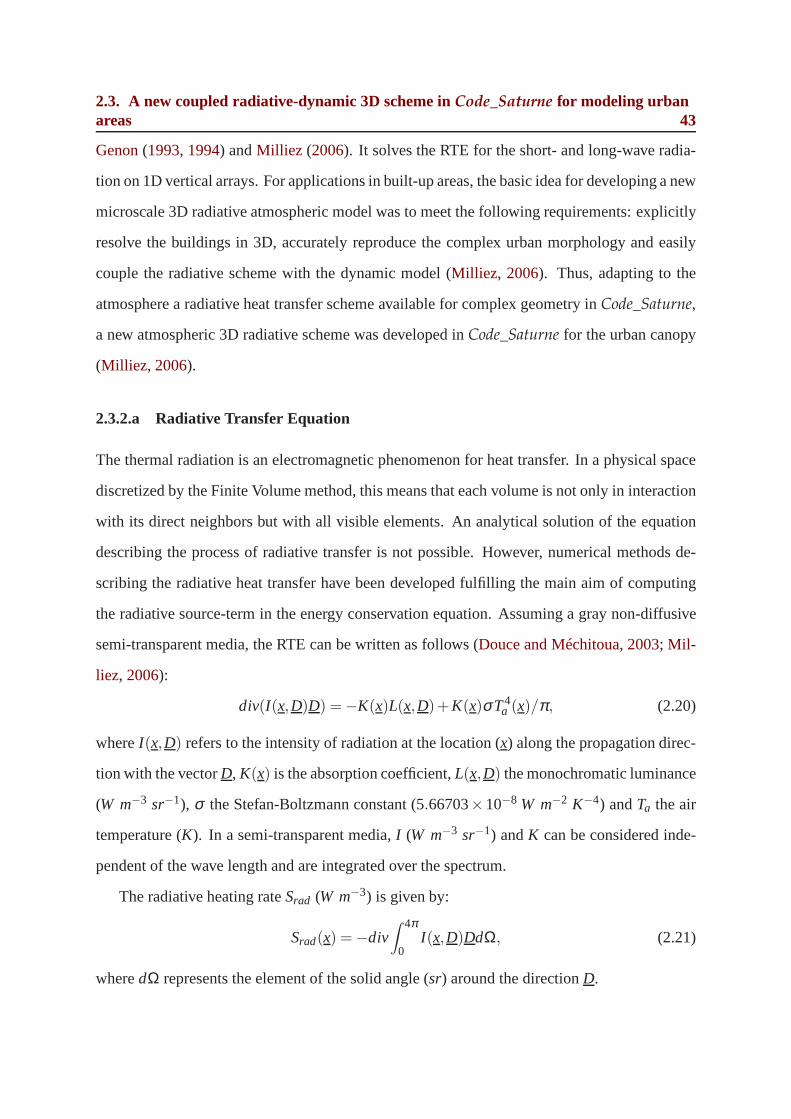
2.3. A new coupled radiative-dynamic 3D scheme inCode_Saturne for modeling urbanareas 43
Genon(1993, 1994) andMilliez (2006). It solves the RTE for the short- and long-wave radia-
tion on 1D vertical arrays. For applications in built-up areas, the basic idea for developing a new
microscale 3D radiative atmospheric model was to meet the following requirements: explicitly
resolve the buildings in 3D, accurately reproduce the complex urban morphology and easily
couple the radiative scheme with the dynamic model (Milliez, 2006). Thus, adapting to the
atmosphere a radiative heat transfer scheme available for complex geometry inCode_Saturne,
a new atmospheric 3D radiative scheme was developed inCode_Saturne for the urban canopy
(Milliez, 2006).
2.3.2.a Radiative Transfer Equation
The thermal radiation is an electromagnetic phenomenon forheat transfer. In a physical space
discretized by the Finite Volume method, this means that each volume is not only in interaction
with its direct neighbors but with all visible elements. An analytical solution of the equation
describing the process of radiative transfer is not possible. However, numerical methods de-
scribing the radiative heat transfer have been developed fulfilling the main aim of computing
the radiative source-term in the energy conservation equation. Assuming a gray non-diffusive
semi-transparent media, the RTE can be written as follows (Douce and Méchitoua, 2003; Mil-
liez, 2006):
div(I(x,D)D) = −K(x)L(x,D)+K(x)σT4a (x)/π, (2.20)
whereI(x,D) refers to the intensity of radiation at the location (x) along the propagation direc-
tion with the vectorD, K(x) is the absorption coefficient,L(x,D) the monochromatic luminance
(W m−3 sr−1), σ the Stefan-Boltzmann constant (5.66703×10⁻⁸ W m−2 K−4) andTa the air
temperature (K). In a semi-transparent media,I (W m−3 sr−1) andK can be considered inde-
pendent of the wave length and are integrated over the spectrum.
The radiative heating rateSrad (W m−3) is given by:
Srad(x) = −div∫ 4π
0I(x,D)DdΩ, (2.21)
wheredΩ represents the element of the solid angle (sr) around the directionD.

44 Chapter 2. Model design
Boundary Conditions For a solid surface, the outgoing long-wave radiative fluxL↑ (W m−2)
at a locationx is composed of a reflected and emitted part under the assumption of a gray,
diffusive radiation of the surface. The boundary conditionfor a surface is given by:
L↑(x) =εσT4
s f c
π+
1− επ
∫ 2π
Ω=0I(x,D) | D.n | dΩ, (2.22)
with ε the emissivity of the surface,Ts f c (K) the surface temperature.
Numerical methods The equation governing radiative transfer is of an integro-differential
type. Some methods such as the zone method and the Monte Carlomethod, may be exces-
sively computing-time demanding and therefore currently not suitable for simulation of fluid
flow, chemical reactions and heat transfer in large simulation domains. Approximate and rapid
solution methods combining accuracy and computational efficiency are preferred especially for
three-dimensional simulations. To resolve the RTE, there are in general two different kinds of
approximate numerical approaches: ray-tracing and differential methods. The essential differ-
ence of these two groups are the directions in which the transport equations are formulated.
• Ray-tracing method: One-dimensional equations along a multitude of individual rays
through the computational domain are solved. The formulation of the equations is made
along straight, arbitrarily oriented rays, which are not inevitably aligned with the coordi-
nate system of the fluid flow. Determining all traces of the rays and cells located along its
way requires either a lot of computational time or a lot of memory. In addition, the vec-
torization and parallelization of the algorithms of ray-tracing radiation models is limited
due to the different lengths of the individual rays (Knaus et al., 1997).
• Differential Methods: They are tools to transform the equation of radiative transfer (Eq.
2.20) into a set of partial differential equations which can be formulated in the Cartesian
coordinate system of the fluid flow. After discretizing the equation with the finite-volume
method, a fast iterative sparse matrix solvers can be used tocompute the solution, and the
code for the differential radiation models can effectivelybe vectorized without significant

2.3. A new coupled radiative-dynamic 3D scheme inCode_Saturne for modeling urbanareas 45
increase of memory. One of the differential methods is the Discrete Ordinates Method
(DOM) (Fiveland, 1984; Truelove, 1987; Liu et al., 2000) which is used in our radiative
model.
2.3.2.b Discrete Ordinates Method (DOM)
In the Discrete Ordinates Method, the radiative transport equation is solved for a set ofn dis-
crete directions (32 or 128). Each direction is associated with a solid angle in which the inten-
sity is assumed to be constant. All solid angles are non-overlapping and spanning the total an-
gle range of 4π. The integrals over the direction are replaced by numericalquadrature weights
summed over each ordinate. In the microscale, we assume thatthe atmosphere is not diffu-
sive. In fact, the angular discretization and the small number of directions make the DOM less
accurate than view factor models. To illustrate this, in Chapter 4, we discuss the advantages
and weaknesses of using DOM in our radiative model through a comparison with SOLENE
model (Miguet and Groleau, 2002) which uses the calculation of view factors or form factors.
We adapted the model to atmospheric radiation. Both short- and long-wave radiation are taken
into account separately. For the short-wave radiation, we distinguish direct and diffuse solar
fluxes. We note that the new radiative scheme is, initially, designed to be applied in the urban
canopy. Consideration of the upper part of the atmosphere isthen taken into account by the
boundary conditions at the top of our domain. Section2.3.2.band2.3.2.cpresent the simple
models for upper boundary conditions when data are not avaible and when not coupled with
the 1D radiative model ofMercure_Saturne.
2.3.2.c Global solar radiation model
When solar rays pass through the atmosphere, there are five main types of radiation-damping
processes: Rayleigh scatering, diffusion by aerosols, absorption by ozone, water vapor absorp-
tion/diffusion and uniformly-mixed gas absorption. The model we use to evaluate the incoming
global solar radiative flux is based on the Bird Clear Sky model (Bird and Hulstrom, 1981) and

46 Chapter 2. Model design
METSTAT model (Maxwell, 1998). The latter one is used to provide the solar radiation data
for the United States.
In clear sky conditions, the direct normal solar fluxSDn (W m−2) is obtained as:
SDn = CS0τrτaτozτwτg, (2.23)
where coefficientC = 0.9751 from METSTAT,S0 = 1370(W m−2) is the solar constant andτr ,
τa, τoz, τw, τg the transmittances.
The solar diffusion flux by the atmosphere is considered to beisotropic and can be expressed
with three terms: Rayleigh diffusionSdr (W m−2), aerosol diffusionSdae(W m−2) and reflection
by the surfaceSdg (W m−2). Each term can be estimated by:
Sdr = 0.79S0cos(Z)τrτaaτozτwτg(1− τr)0.5
1−m+m1.02, (2.24)
Sdae= 0.79S0cos(Z)τrτaτozτwτg(1− τad)Fc
1−m+m1.02, (2.25)
Sdg = (SDncos(Z)+Sdr +Sae)αgαs
1−αgαs, (2.26)
with Z (rad) the sun zenith angle,τaa andτad the transmittance due to aerosol absorption and
scattering, respectively,mair mass (kg m−3) andFc the ratio of the forward-scattered irradiance
to the total scattered irradiance due to aerosols,αg averaged ground albedo,αs clear sky or
atmospheric albedo.
All above expressions are in accordance withMilliez (2006) with the following modifica-
tions. First, proposed byYang et al.(2001), a different expression for the air mass is used:
m= (1−0.0001zs)/[sin(h)+0.15(57.296h+3.885)−1.253], (2.27)
wherezs (m) is ground level andh (rad) is the altitude angle of the sun.
Secondly, in equation2.24, the expression of the transmittance due to aerosol absorption
τaa is
τaa = 1−E1(1−m+m1.06)(1− τa), (2.28)
with E1 the constant used in the Bird model associated with aerosol absorption. After testing,
the suggested the values ofFc = 0.84 andE1 = 0.1 as inBird and Hulstrom(1981) are more
appropriate for our simulations than other suggested values.

2.3. A new coupled radiative-dynamic 3D scheme inCode_Saturne for modeling urbanareas 47
2.3.2.d Incident long-wave radiation model
Incoming longwave radiation,L↓ (W m−2) is generally expressed in terms of the Stefan-
Boltzmann Law:
L↓ = εatmσT4atm = εclrFσT4
atm, (2.29)
whereεatm = εclrF is referred to as the effective or apparent emissivity and generally varies
between roughly 0.7 for clear skies to close to unity for completely overcast skies, withεclr the
clear-sky atmospheric emissivity.F (always≥ 1) is a cloud factor expressing the increase in
clear-skyL↓ due to cloud emission, andTatm (K) is the effective atmospheric temperature.
The simple model implemented inCode_Saturne is after byPrata(1996): Tatm is approx-
imated by the air temperatureTa at reference height close to the surface, andεclr is estimated
by:
εclr = 1− [1+w exp(−(1.2+3w)0.5)] (2.30)
where the precipitation water contentw equals 46(ea/Ta) with ea (Pa) the water vapor pressure.
2.3.3 Surface temperature models
The surface temperatureTs f c (K) is a key control for energy exchanges at the urban surfaces,
particularly for the net long-wave radiation and turbulentenergy fluxes. The surface tempera-
ture is controlled by the balance between the external net fluxes and the conductive heat flux
through the wall, internal to the external. As a first step in our development, a simple sur-
face temperature model, the force-restore approach (Deardorf, 1978) has previously been im-
plemented inCode_Saturne by Milliez (2006). Because of the limiting hypotheses of this
approach and in order to more accurately calculate the surface temperature of buildings, I ad-
ditionally test in this work a one-dimensional surface temperature approach, called hereafter
the wall thermal model. Thus, the surface temperature in thesimulations is computed from
either the force-restore scheme or the wall thermal scheme.In this section, we briefly describe
these two approaches. A comparison of these two surface temperature models with simulation

48 Chapter 2. Model design
results and observation data is presented in Chapter 3. Actually, a hybrid approach taking the
advantages of both the force-restore method and wall thermal scheme has also been tested at
the end of the this work (see Chapter 6).
2.3.3.a The Force-restore method
The Force-restore approach (Deardorf, 1978) is commonly used in order to calculate the ground
temperature in atmospheric models and is considered a very useful tool. In this approach, a
prognostic equation for temperature is used to reproduce the response to periodic heating of the
soil. The model is based on an analytical solution of a two-layer decomposition of a material
considered homogeneous. The deep soil temperature calculation appears in the restore term
of the force-restore equation. This model has been extendedto urban surfaces (Johnson et al.,
1991; Dupont and Mestayer, 2006). Hence, the prediction of the surface temperature is made
by using following equation:
∂Ts f c
∂ t=
√2ωµ
(L∗ +S∗−QH)−ω(Ts f c−Tg/b) (2.31)
whereω (Hz) is the earth angular frequency,L∗ (W m−2), S∗ (W m−2), QH (W m−2) are
respectively net long-wave, net short-wave, and sensible heat flux,µ (J m−2 s−0.5 K−1) the
thermal admittance andTg/b (K) either deep soil or internal building temperature.
This extension nevertheless supposes well insulated buildings with a nearly constant inter-
nal temperature and homogeneous material.
2.3.3.b Wall thermal model
Neglecting the anthropogenic flux and the latent heat flux terms in equation1.1, the simplified
energy balance reads:
Qcond+QH = L∗ +S∗. (2.32)
One-dimensional conduction within the patch substrate is bounded by surface energy ex-
changes at the patch surface and by the internal building energy exchanges or a deep-soil tem-
perature at the substrate base. In the hypothesis of a singlelayer to express the conduction term,

2.3. A new coupled radiative-dynamic 3D scheme inCode_Saturne for modeling urbanareas 49
equation2.32reads after expression of each term:
λe(Ts f c−Tint)+hf (Ts f c−Ta) = ε(La +Le−σT4
s f c)+(1−α)(SD +Sf +Se) (2.33)
whereλ (W K−1 m−1) is the average thermal conductivity of the wall,e(m) the thickness of the
wall, Tint (K) the internal building or deep soil temperature,hf (W m−2 K−1) the heat transfer
coefficient calculated from equation2.36andTa the external air temperature (K).
2.3.3.c Internal building temperature model
In our model, the internal building temperature is initially set to a constant and computed by
averaging the diurnal temperatures of all the building surfaces. However, in case the building
is not well insulated, the variation of the internal building temperature can be important and
may have a significant impact on the surface temperature (seeChapter 3). Moreover, the inter-
nal temperature is rarely measured in the experiment. In order to more accurately model the
internal temperature and take into account its variation, it is computed with an incremental-
adjustment method afterMasson et al.(2002) and similarly used byKrayenhoff and Voogt
(2007):
Tn+1int = Tn−1
int (τ −∆ t
τ)+T(
∆tτ
), (2.34)
whereTn+1int (K) andTn−1
int (K) are the computed internal temperatures at the following and
previous time step respectively,∆t is the time step (s), τ (s) refers to the number of seconds in
a day, andT (K) is the average over all the surface temperatures computed at time stepn.
A potential improvement would involve accounting for the full internal building energy
balance proposed byMills (1996) and also used in SOLENE (Miguet and Groleau, 2002), but
is not included at present. In order to improve the results, we can replace in Eq.2.34T from
the calculation with the average of the measured surface temperatures, if avaible. The latter is
included as a user-controlled option in our model.
It should be noted that a constant internal building temperature effectively represents the
inclusion of an anthropogenic heating term when the external air is cooler than the interior one

50 Chapter 2. Model design
(Arnfield, 2003). On the other hand, it is an artificial heat sink when the external air is warmer
than the building interior. The mean building surface temperatures are quite sensitive to the
internal building temperature evolution, both in terms of magnitude and time-evolution of the
diurnal pattern. I will further discuss this point in Chapter 3.
2.3.3.d Brightness temperature
Many comparisons with observations are made in terms of brightness surface temperatures
since it is the quantity measured by infrared thermometers (IRT) whilst model-calculated sur-
face temperatures result from the solution of the surface energy balance (see Chapter 6). Bright-
ness surface temperatures account for the surface emissivity and multiple reflections (together,
effective emissivity) that are inherent in the observations. Surface brightness temperature (Tbr
(K)) is defined as the temperature that yields to an emitted broadband thermal radiance equiva-
lent to the sum of the true broadband emitted radiance (with reduction due to gray body emis-
sivity) and the broadband reflected radiance (after multiple reflections on canyon surfaces)
(Krayenhoff and Voogt, 2007; Moscicki, 2007; Hénon, 2008):
Tbr =4
√εT4
s f c+(1− ε)L ↓
σ. (2.35)
2.3.4 Convection model
The surface convective heat flux must be computed to both solve the surface energy balance
(Eq.1.7) and determine the surface-air thermal gradient and therefore turbulent transport. In
Code_Saturne, the convective heat transfer is computed in 3D for each surface patch. The
buildings are explicitly defined in our simulations. Therefore, the detailed representation of the
surface allows for a more complex 3D spatial representationof wind speed, turbulence, and
temperature than simple canopy averages or vertical profiles. We use a rough wall boundary
condition, based on the logarithmic law modified by the stratification. Usually these modified
laws are based on the Monin-Obukov similarity but are implicit and therefore need to be solved

2.3. A new coupled radiative-dynamic 3D scheme inCode_Saturne for modeling urbanareas 51
iteratively. Here we use an explicit approach based on the work of Louis (1979) and described
in Musson-Genon et al.(2007).
The heat transfer coefficienthf in Eq.1.7 is computed for each solid sub-facet, depending
on the local friction velocityu∗ (ms−1):
hf =ρCpu∗κ fh
σt ln(d+z0
z0T
)√
fm
, (2.36)
whereCp is specific heat (J kg−1 K−1), u∗ is the friction velocity,κ is von Karman constant,
σt the turbulent Prandtl number,d is the distance of the cell center (m) to the wall, z0 the
roughness length (m), z0T the thermal roughness length (m), fm and fh are theLouis (1979)
stability functions which take a value of 1 for neutral conditions. For vertical walls, the neural
conditions are applied.
In Chapter 3, I discuss different approaches to model the heat transfer coefficient.


CHAPTER 3
Micrometeorological modeling of radiative
and convective effects with a building
resolving code: published in Journal of
Applied Meteorology and Climatology,
(2011) 50, 1713–1724
In the previous chapter, we introduced the new coupled radiative-dynamic 3D scheme in
Code_Saturne. To ensure modeling accuracy, validating the model resultswith experimen-
tal data is necessary. The paper presented here shows the first evaluation of the coupling with
data from the Mock Urban Setting Test (MUST) field experiment. In MUST, the buildings are
idealized by an array of shipping containers. We have simulated a moderate wind speed day by
modeling a detailed flow field. The simulations results showed a significant impact of the con-
vective flux on the surface temperatures. Furthermore, the discussion about the comparison of
three schemes of increasing complexity for predicting surface sensible heat flux also emphasize
the contribution of modeling the detailed flow field.


Micrometeorological Modeling of Radiative and Convective Effectswith a Building-Resolving Code
YONGFENG QU, MAYA MILLIEZ, LUC MUSSON-GENON, AND BERTRAND CARISSIMO
Teaching and Research Center in Atmospheric Environment (CEREA), Champs-sur-Marne, France
(Manuscript received 10 August 2010, in final form 14 March 2011)
ABSTRACT
In many micrometeorological studies with computational fluid dynamics, building-resolving models usually
assume a neutral atmosphere. Nevertheless, urban radiative transfers play an important role because of their
influence on the energy budget. To take into account atmospheric radiation and the thermal effects of the
buildings in simulations of atmospheric flow and pollutant dispersion in urban areas, a three-dimensional (3D)
atmospheric radiative scheme has been developed in the atmospheric module of the Code_Saturne 3D
computational fluid dynamic model. On the basis of the discrete ordinate method, the radiative model solves
the radiative transfer equation in a semitransparent medium for complex geometries. The spatial mesh dis-
cretization is the same as the one used for the dynamics. This paper describes ongoing work with the de-
velopment of this model. The radiative scheme was previously validated with idealized cases. Here, results of
the full coupling of the radiative and thermal schemes with the 3D dynamical model are presented and are
compared with measurements from the Mock Urban Setting Test (MUST) and with simpler modeling ap-
proaches found in the literature. The model is able to globally reproduce the differences in diurnal evolution
of the surface temperatures of the different walls and roof. The inhomogeneous wall temperature is only seen
when using the 3D dynamical model for the convective scheme.
1. Introduction
Interest in urban climatology has increased in the past
decade. It corresponds to the thermal and dynamical air-
flow response to the urban system solicitations, resulting
in radiative transfers and convective exchanges within the
urban air and with the building walls (Grimmond and
Oke 1999; Arnfield 2003). In the past few years, numer-
ical studies have been conducted to solve the surface
energy balance (SEB) in urban canopies, with different
degrees of simplification, using either an integrated rep-
resentation of the urban canopy (Masson 2000) or a three-
dimensional approach (Mills 1996; Miguet and Groleau
2002; Kanda et al. 2005; Krayenhoff and Voogt 2007;
Gastellu-Etchegorry 2008; Asawa et al. 2008). Those
models share the following parameterizations in their
design: the schemes possess separate energy budgets
for roofs, roads, and walls; radiative interactions be-
tween roads and walls are explicitly treated.
The Town Energy Balance (TEB) scheme of Masson
(2000) consists of a facet-averaged scheme with one ge-
neric roof, one generic wall, and one generic road. The
advantage of the integrated resolution is that few in-
dividual SEBs need to be resolved and therefore com-
putation time is kept low, with a simple approach to
model the inner-canopy wind flow. TEB has been shown
to reproduce accurately the SEB from regional to me-
soscale and urban scales (Masson et al. 2002; Lemonsu
et al. 2004). Mills (1996) developed the Urban Canopy-
Layer Climate Model, which has a detailed representation
of the canyon with a highly simplified wind parameter-
ization. The ‘‘SOLENE’’ (Miguet and Groleau 2002) and
3D-Computer Aided Design (Asawa et al. 2008) models
are based on a realistic description of the canopy struc-
ture using a geometrical 3D surface model assigning ra-
diative and thermal properties to each subfacet of the
model and a constant transfer coefficient for each class
of elements. The model is originally designed for simu-
lating sunshade, natural lighting, and heat transfers for
architectural purposes. The Discrete Anisotropic Radia-
tive Transfer (DART) model (Gastellu-Etchegorry et al.
2004) simulates the radiative transfer in the whole op-
tical domain simultaneously in the atmosphere and in
Corresponding author address: Yongfeng Qu, Teaching and Re-
search Center in Atmospheric Environment (CEREA) (ENPC/EDF
R&D), 6–8 avenue Blaise Pascal, 77455 Champs-sur-Marne, France.
E-mail: [email protected]
AUGUST 2011 Q U E T A L . 1713
DOI: 10.1175/2011JAMC2620.1
2011 American Meteorological Society

the urban and vegetated landscapes, with or without
topography. A major feature of DART is that it can
simulate images in the plane of the sensor, for differ-
ent altitudes from the bottom to the top of the atmo-
sphere. The new version of the DART model, DART-EB,
(Gastellu-Etchegorry 2008) includes an energy balance
component. In the case of urban canopies, turbulent fluxes
and conduction are computed with classical boundary
layer laws, using the equations of the TEB model (Masson
2000). The Simple Urban Energy Balance Model for
Mesoscale Simulations (SUMM; Kanda et al. 2005),
which represents the urban canopy with an infinitely
extended regular array of uniform buildings, is more
adapted for the mesoscale. The Temperatures of Urban
Facets in 3D (TUF-3D) model (Krayenhoff and Voogt
2007) uses the radiosity approach based on interpatch
view factors to model radiative exchange between the
identical square patches that compose the simplified 3D
urban geometry. An exponential inner-canopy wind
speed profile is employed. TUF-3D has applications in
both surface temperature distributions and thermal re-
mote sensing anisotropy at several scales.
Previously described models have all put a strong
emphasis on radiative exchanges but not on a detailed
flow field. In this work, in addition to the above appli-
cations, we are also interested in applying the model to
pollutant dispersion in low–wind speed conditions, when
the thermal effects have a strong influence on the flow.
To model the airflow in the urban canopy in non-
neutral conditions more accurately and to take into ac-
count the 3D convective exchanges, we developed a 3D
microscale radiative model coupled with a 3D compu-
tational fluid dynamics (CFD) code for complex geom-
etries to simulate dynamics and thermodynamics of the
urban atmosphere (Milliez 2006). Differing from other
radiative models that calculate the view factors to esti-
mate the incoming radiative fluxes on urban surfaces,
our model directly solves the 3D radiative transfer
equation in the whole fluid domain. This approach al-
lows us to determine the radiation flux not only on the
facets of the urban landscape but also in each fluid grid
cell between the buildings. The difference could become
important in the case of smoke or fog between the
buildings. The model was evaluated with idealized cases,
using as a first step a constant 3D wind field (Milliez et al.
2006). The purpose of the work presented here is to
study the full radiative–dynamical coupling, using an
evolving 3D flow field. First we present the model, and
then we discuss in detail the results of the full coupling.
We further discuss the influence on the surface tem-
perature of the internal building temperature and the
wall thermal modeling, comparing the 3D resolution
with the approaches used in other models.
2. Equations and model design
As a key parameter, surface temperature Tsfc is de-
termined by the SEB, which governs the energy ex-
change processes between each urban surface and the
atmosphere (Fig. 1). It is given by
Qcond 1 QH 5 L* 1 S*, (1)
where Qcond is the conductive heat flux (W m22) within
the building or the ground subsurface that links the
surface temperature to the internal-building or the deep-
soil temperature, QH is the sensible heat flux (W m22)
and depends on the local wind intensity, S* is the net
shortwave radiative flux (W m22), and L* is the net
longwave radiative flux (W m22). We neglect in this study
the other energy fluxes such as the anthropogenic flux and
the latent heat flux. In our model the advection fluxes are
taken into account by the full resolution of the flow field.
a. CFD model
To solve the dynamics and therefore to resolve the
QH term explicitly, simulations are performed with the
3D open-source CFD code known as Code_Saturne
(Archambeau et al. 2003), which can handle complex
geometry and complex physics. The flow features in
built-up areas make the modeling within the urban can-
opy difficult. Some typical effects that we have to handle
are 3D vortices behind the buildings, high wind speed
near the edges of the upwind face, wake effects, and
modified turbulence.
FIG. 1. Schematic representation of the energy exchanges at an
urban surface (cross section of a building) (S*: net shortwave ra-
diative flux; L*: net longwave radiative flux; QH: sensible heat flux;
Qcond: conduction heat flux; TW: wall surface temperature; Tint:
internal building temperature).
1714 J O U R N A L O F A P P L I E D M E T E O R O L O G Y A N D C L I M A T O L O G Y VOLUME 50

In this work, we use the atmospheric module of Code_
Saturne, described in detail in Milliez and Carissimo
(2007), which takes into account the larger-scale me-
teorological conditions and the thermal stratification of
the atmosphere. In our simulations, we use a Reynolds-
averaged Navier–Stokes (RANS) approach with a k–«
turbulence closure. The numerical solver is based on
a finite-volume approach for collocated variables on
an unstructured grid. Time discretization is achieved
through a fractional step scheme, with a prediction–
correction step.
b. Radiative model
A new atmospheric 3D radiative scheme was devel-
oped in Code_Saturne for the urban canopy (Milliez
2006). We have adapted to the atmosphere a radiative
heat transfer scheme available for complex geometry in
Code_Saturne that solves the radiative transfer equa-
tion for a gray nondiffusive semitransparent media:
div[I(x, D)D] 5 2K(x)L(x, D) 1 K(x)sT4a (x)/p, (2)
where I(x, D) is the intensity of radiation at the point x
and for the propagation direction D, K(x) is the absorp-
tion coefficient, L(x, D) is the luminance (W m23 sr21),
and Ta is the air temperature (K). In a semitransparent
media, I (W m23 sr21) and K can be considered to be
independent of the wavelength and are integrated over
the spectrum. The rate of radiation heating Srad (W m23)
is then given by
Srad 5 2div
ð4p
0I(x, D)D dV, (3)
where dV is the element of the solid angle (sr) around
the direction.
1) DISCRETE ORDINATE METHOD (DOM)
To solve the radiative transfer equation, we chose
the discrete ordinate method (Fiveland 1984; Truelove
1987; Liu et al. 2000), which is based on the directional
propagation of the radiative wave. The spatial discretiza-
tion uses the same mesh as the CFD model. The angular
discretization has two resolutions: 32 or 128 directions.
2) SHORTWAVE AND LONGWAVE RADIATION
As is usually done, we separate the atmospheric ra-
diation into shortwave and longwave radiation. The to-
tal incoming and outgoing shortwave radiative fluxes for
each solid surface are given by
SY 5 SD 1 Sf 1 Se and (4)
S[ 5 aSY, (5)
where SY and S[ are respectively the incoming and
outgoing shortwave radiative fluxes (W m22), SD
is the direct solar flux (W m22), Sf is the solar flux
diffused by the atmosphere above our simulation do-
main (W m22), Se is the flux diffused by the environ-
ment, that is, resulting from the multireflections on
the other subfacets (W m22), and a is the albedo of the
surface.
We express the longwave radiation flux for each sur-
face as
LY 5 La 1 Le and (6)
L[ 5 «sT4sfc 1 (1 2 «)(La 1 Le), (7)
where LY and L[ are respectively incoming and out-
going longwave radiation flux (W m22), « is emissivity
of the surface; s is the Stefan–Boltzmann constant
(5.667 03 3 1028 W m22 K24), Tsfc is the surface tem-
perature (K), and La and Le are the longwave radiation
flux from the atmosphere and from the multireflection
on the other surface. As the first step of validation, we
assume that, at the scale of our simulations, the atmo-
sphere between the buildings is transparent and set the
absorption coefficient to 0 for both the longwave and
shortwave radiation.
3) SURFACE TEMPERATURE MODEL
The force–restore approach (Deardorf 1978) is com-
monly used to calculate the ground temperature in
meteorological models. This approach is considered
to be a very useful tool because a prognostic equation
for temperature is used to reproduce the response to
periodic heating of the soil. This model has been ex-
tended to urban surfaces (Johnson et al. 1991; Dupont
and Mestayer 2006). This extension nevertheless sup-
poses well-insulated buildings with a nearly constant
internal temperature and homogeneous material. In our
model, the force–restore method has been available for
some time in simple geometries and has been extended
to complex geometries. Because of the limiting hypoth-
eses built into the method, however, especially concern-
ing the deep-soil temperature, we have also tested a
simple wall thermal model with a given thickness and an
average thermal conductivity.
(i) Force–restore model
The force–restore model is based on a two-layer de-
composition of a material considered to be homogeneous:
the surface-layer temperature Tsfc responding to external
forcing and the deeper layer independent of the diurnal
variation. It reads
AUGUST 2011 Q U E T A L . 1715

›Tsfc
›t5
ffiffiffiffiffiffi2vp
m(L* 1 S* 2 QH) 2 v(Tsfc 2 Tg/b), (8)
where v is the Earth angular frequency (Hz), m is the
thermal admittance (J m22 s20.5 K21), and Tg/b is either
deep-soil or internal building temperature (K).
(ii) Wall thermal model
This model solves the conduction equation to com-
pute the wall temperature. It reads, after expressing
each term in Eq. (1), as
l
e(Tsfc 2 Tint) 1 hf (Tsfc 2 Ta)
5 «(La 1 Le 2 sT4sfc) 1 (1 2 a)(SD 1 Sf 1 Se), (9)
where l is the average thermal conductivity of the
wall (W K21 m21), e is the thickness of the wall (m),
Tint is the internal air temperature (K), hf is the heat
transfer coefficient (W m22 K21) computed from lo-
cal flow parameters, and Ta is the external air tem-
perature (K).
4) INTERNAL BUILDING TEMPERATURE
In a real building with good insulation, the variation
of the internal building temperature is small. In the ex-
periment we simulate (see section 3), however, the
buildings are represented by poorly insulated shipping
containers. In this case, the variation of the internal
temperature is important and has a great influence on
the surface temperature. The internal temperature was
not measured in the experiment, however and we com-
puted it with one of the following methods.
(i) Constant T
In this case, the internal building temperature is set to
a constant and is computed by averaging the diurnal
temperatures of all of the building surfaces.
(ii) Evolution equation
A temperature evolution equation, as in Masson et al.
(2002), is used to represent the temperature inside the
buildings:
Tn11int 5 Tn21
int
t 2 Dt
t
1 T
Dt
t
, (10)
where Tn11int and Tn21
int are the computed internal tem-
peratures (K) at the following and previous time step,
respectively, Dt is the time step (s), t is the period (equal
to 1 day; (s), and T is the average over all of the surface
temperatures (K) computed at time step n.
(iii) Evolution equation with T interpolated frommeasurements
We use the previous formula [Eq. (10)] and replace T
from the calculation with the average of the measured
surface temperatures.
Figure 2 compares the northeast wall surface tem-
perature of a shipping container computed with the
three different internal temperature models and the
measurements from the Mock Urban Setting Test ex-
periment (see section 3). The value of the constant av-
erage internal temperature model is 248C, which is
approximately 2 times the initial values in the other two
internal temperature models. Before sunrise, this high
value of the constant internal temperature induces a
too-rapid heating of the northeast wall. At midday, the
constant internal temperature is too low to account for
the warming of the surface by the interior air heated by
the other sunlit surfaces of the container. Computing the
internal temperature with an evolution equation model
decreases the heating of the northeast wall before sun-
rise and improves the results at midday. The differences
in the results obtained by using the two evolution equa-
tion models (with T from computation and T from
measurements) are small, which was expected because
Dt/t is small. Nevertheless, using the observed average
temperature slightly improves the results, especially
during the night, when the atmospheric radiative fluxes
decrease. The same conclusion applies for the other sides
of the containers, which are not shown here. We stress that
this may be relevant only in the case of metal containers.
FIG. 2. Comparison of the diurnal evolution of the surface tem-
perature of a northeast-oriented wall computed with three differ-
ent models for the internal temperature (times signs: surface
temperature from the measurements; dashed line: taking a con-
stant internal building temperature; solid line: taking an evolution
equation; filled circles: taking the average surface temperature
from the measurements and then using the result in the evolution
equation).
1716 J O U R N A L O F A P P L I E D M E T E O R O L O G Y A N D C L I M A T O L O G Y VOLUME 50

5) CONVECTION MODEL
The thermal energy equation of the flow must be
solved, both to determine stratification effects on verti-
cal turbulent transport and to estimate the surface–air
thermal gradient that controls convective heat transfer.
The sensible heat flux QH is given by
QH 5 hf (Ta 2 Tsfc). (11)
Detailed comparisons between different approaches to
model the heat transfer coefficient will be discussed in
section 5. Our CFD model solves in 3D the RANS
equations in the entire fluid domain. In our simulations,
we use a rough-wall boundary condition. The hf is com-
puted for each solid subfacet, depending on the local
friction velocity:
hf 5rCpu*kfm
st ln
d 1 z0
z0T
! ffiffiffiffifh
q , (12)
where r is flow density (kg m23), Cp is specific heat
(J kg21 K21), u*
is the friction velocity, k is the von
Karman constant, st is the turbulent Prandtl number,
d is the distance (m) to the wall, z0 is the roughness
length (m), z0Tis the thermal roughness length (m), and
fm and fh are the Louis (1979) stability functions.
3. Study case: The Mock Urban Setting Test
a. Configuration of the experiment
The Mock Urban Setting Test (MUST; Biltoft 2001;
Yee and Biltoft 2004) conducted in the Utah desert is
a near-full-scale experiment that consists of measure-
ments in an idealized urban area represented by 120
shipping containers (length L 3 width W 3 height H 5
12.2 m 3 2.42 m 3 2.54 m) arranged in a regular ar-
ray. MUST has already been used to validate dynamics
and dispersion models (Brook et al. 2002; Hanna et al.
2002; Camelli et al. 2005; Milliez and Carissimo 2007,
2008). Because temperature data are also provided, we
used the MUST field experiment to study in detail the
dynamic–radiative coupling. We focused our study on
one instrumented container within the array, and there-
fore the computational domain was reduced to three rows
of three containers (Fig. 3).
From the MUST experiment, we selected the day of
25 September 2001. Despite a fairly strong wind (Umean 5
7 m s21), we selected this day because it has already been
partly simulated for studies on dispersion (Milliez and
Carissimo 2007) and moreover because a complete 24-h
dataset for the upstream wind and the surface tempera-
ture was available (which was not the case for other days).
During this day (Fig. 4), the wind velocity varied from
Umin 5 3 m s21 to Umax 5 11.5 m s21 and the average
diurnal air temperature was about 248C (measured at
10 m). For our coupling study, the wind speed may be
a little high to test strong radiative effects on the airflow,
but it emphasizes the convective effects on the surface
temperature.
b. Boundary conditions and surface parameters
Table 1 gives the parameters used in the simulation.
To be consistent with the experiment, the wind inlet
boundary conditions are determined from measure-
ments, using a meteorological file that contains the wind
velocity, turbulence kinetic energy, dissipation rate, and
temperature profiles for every 2 h. The variation of the
deep-soil temperature is neglected. The internal build-
ing temperature is computed by the evolution equation
with T from measurements. We take the same value
of the roughness length z0 as in Eichhorn and Balczo
(2008). The thermal roughness length z0Tis considered
to be 1/10 of z0 (Garratt 1992). Because some thermal
properties were not determined during the experiment,
their values were taken from the literature: we took the
values of the albedo and emissivity of the wall to be
those of corrugated iron (Oke 1987). The thermal ad-
mittance was taken assuming an insulating material in
the walls, as observed in some pictures. The ground
albedo as that was input to the model was evaluated
from the incoming and outgoing solar fluxes measured
upstream by pyranometers and depends on the zenith
angle.
FIG. 3. Mesh of the domain and the subdomain for the 0.8 m 3
0.5 m 3 0.5 m resolution.
AUGUST 2011 Q U E T A L . 1717

c. Numerical sensitivity
Before starting our simulations, we performed a nu-
merical sensitivity study for the grid size, the number
of directions in the discrete ordinate method, and the
radiative time step. We focus here on the radiative as-
pects because a sensitivity study of the dynamical part
has already been performed (Milliez and Carissimo 2007,
2008).
Figure 5 shows surface temperature evolution with
grids of different resolutions. The fine (;55 000 cells)
and the refined grids (;173 000 cells) give similar re-
sults, and the coarse grid (;4000 cells) overestimates
or underestimates temperatures, and therefore the fine
grid is used in the remaining simulations. Among these
three resolutions, we also observe that the coarse grid
largely underestimates the southwest surface tempera-
ture at about 16 h. The reason is that this surface re-
ceives less direct solar flux in the coarse grid than in the
fine grid as shown on (Fig. 6). In addition, the thermal
boundary layer close to the heated surface may need
a sufficient resolution to be captured in such a canopy.
FIG. 4. Meteorological data at 10 m from the MUST experiment
for 25 Sep 2001: (a) wind speed (m s21), (b) meteorological wind
direction (8), and (c) wind (air) temperature (8C).
TABLE 1. Parameters employed in the MUST simulations, with
Zref being the reference height for forcing data, Uref being the
initial wind speed at Zref, and u being the initial wind angle. Soil z0,
wall z0, and roof z0 are respectively the roughness length for mo-
mentum of soil, walls, and roofs. Soil z0T
, wall z0T
, and roof z0T
are respectively the roughness length for heat of soil, walls, and
roofs; aS, aW, and aR are respectively the shortwave albedo of soil,
walls, and roofs; «S, «w, and «R are respectively the longwave
emissivity of soil, walls, and roofs; mS, mW, and mR are respectively
the admittance of soil, walls, and roofs; Tair is the initial air tem-
perature at Zref; TS and TSint are respectively the initial soil tem-
perature and deep-soil temperature; TTop, TNW, TSE, TNE, and TSW
are initial individual surface temperature; TWint and TRint are re-
spectively the building and roof internal temperature.
Parameter Unit Value
Dynamic
Time step s 0.1
Zref m 10
Uref m s21 4.27
u 8 135
Soil z0 cm 2
Wall z0 5 roof z0 cm 0.2
Radiative
Time step min 5
Soil z0 cm 0.2
Wall z0T5 roof z0T
cm 0.02
aS From measurements
aW 5 aR 0.1
«s 0.8
«w 5 «R 0.13
mS J m22 s20.5 K21 1200
mW 5 mR J m22 s20.5 K21 1600
Initial values
Tair 8C 16.45
TS 8C 15.88
TSint 8C 24.28
TTop 8C 9.28
TNW 8C 10.50
TSE 8C 11.68
TNE 8C 11.87
TSW 8C 12.37
TWint 5 TRint 8C 11.11
1718 J O U R N A L O F A P P L I E D M E T E O R O L O G Y A N D C L I M A T O L O G Y VOLUME 50

Hence, we verified that the fine resolution (0.5 m) in the
canopy is enough to reproduce a thermal boundary layer
thickness of about 2 m.
In our model, the DOM was implemented with two
angular discretizations: 32 or 128 directions, which in-
fluence the prediction of the diffuse solar flux and the
infrared flux. In this case, the results obtained with 32
directions are very close to the ones with 128 directions,
but the calculation is faster by a factor of 5. So we took
32 directions in the remaining simulations. A time step
was introduced for the radiative scheme that is different
from the one used for the dynamics. We have tested
several radiative time steps: 1, 5, 15, and 30 min and 1 h
for a diurnal cycle simulation. The resulting difference
between a time step of 1 min and 5 min is small, being
less than 18C. We considered that 5 min was an optimum
radiative time step for our simulations. The time step for
the dynamics was set to 0.1 s after Milliez and Carissimo
(2007). The 24-h simulation in parallel computing on
a workstation with eight processors took approximately
4.5 days. We have also tested a dynamical time step of
0.5 s, which reduces the computational time to less than
1 day: the results are close to the ones obtained with
a dynamical time step of 0.1 s from 0 to 9 h, but after
10 h an important difference (12%–30%) appears when
the wind speed exceeds 6 m s21 (Fig. 4). In cases in
which the wind speed is small, we could set up the dy-
namical time step to 0.5 s to reduce significantly the
CPU time. The full radiative–dynamic coupling remains
computationally expensive, in comparison with simpler
models, but at this stage the model is intended for re-
search and not for operational applications.
4. Results
a. Simulation of 25 September
Figure 7 shows the evolution of modeled and measured
surface temperatures using the force–restore method,
with two modeling approaches: 1) radiative only and no
convection model (meaning with the convective flux set
to zero) and 2) coupled radiative and dynamical model.
The diurnal evolutions of the surface temperatures of
the top face, southeast face, and northeast face are cor-
rectly reproduced by our coupled model. For the north-
west face and the southwest face, the simulations show
a delay in the morning warming. This delay in warming
can be explained by the conduction between the con-
tainer walls, which contributes to the fast warming in the
northwest and southwest faces before they are in the sun
but which is neglected in the simulations. In addition, this
delay may be inherent to the force–restore method, which
overestimates in this case the relaxation to the internal
temperature and therefore enhances the thermal inertia.
This inertia effect is also observed after sunset for the
simulated northwest surface temperature, which shows
a delay in cooling. In the afternoon when the atmospheric
radiative forcing increases, however, the modeled surface
temperatures compare well to the measurements. The
comparison with measurements shows a large improve-
ment for the coupled model as compared with the radia-
tive-only model, underlining the importance of accurately
including the effect of convection in microscale modeling.
b. Sensitivity to the surface parameters and surfacetemperature models
The values of the surface parameters were taken from
the literature. The values for the thermal properties of
FIG. 5. Surface temperature evolution during a diurnal cycle for
different mesh resolutions: dashed lines: coarse grid of ;4000 cells;
solid lines: fine grid of ;55 000 cells; filled circles: refined grid
about 173 000 cells.
FIG. 6. Vertical cross section of the direct solar flux in the fluid
domain around a building at 16 h for different spatial resolutions:
(a) coarse grid and (b) fine grid.
AUGUST 2011 Q U E T A L . 1719

metal cover a wide range (Oke 1987), however, and we
performed a sensitivity study of the variation of the
surface temperatures when varying the parameters in
the range given by the literature. Table 2 illustrates that
a change in albedo, emissivity, or admittance, in the
range given by the literature, can make a difference of
about 18–108C for the surface temperature. Because the
southeast wall is the most exposed to the sun all day, the
deviation of the temperature on this wall is the most
important.
The results presented above were obtained by using
the force–restore method and are now compared with
those obtained with the wall thermal model [see section
2b(3)]. The emissivity was chosen after Oke (1987) for
corrugated iron. Because some of the containers in the
MUST array were painted, we also made a test taking
a much higher emissivity (i.e., 0.9). It results in a de-
crease in surface temperature. This decrease is greater
when using the force–restore method, about 108C for the
southeast wall and 58C for rest of the walls. For the wall
thermal model, the influence of higher emissivity on the
surface temperature is less significant, the difference
being less than 28C for all of the faces. This is can be
explained the fact that the internal temperature has
a greater influence than the other surface parameters.
The wall thermal model also requires the characteristics
of the surface material and the thickness and the thermal
conductivity of the wall which were not provided in
the data. When choosing a thermal conductivity of 26
W K21 m21 for the walls, the resulting conduction re-
mains too high, resulting in an homogenization of the
temperature of the five walls (not shown here). To im-
prove the comparisons with the observations, we ad-
justed the value of the conductivity to 6 W K21 m21,
which is not that of pure metal, but may be set by as-
suming an insulating material in the walls. In Fig. 8, we
display the evolution of the northwest wall tempera-
ture where we used a conductivity of 6 W K21 m21 and
FIG. 7. Evolution of surface temperature of (a) roof (top), (b)
northwest, southeast, (c) northeast, and southwest faces modeled
using the force–restore method during a diurnal cycle (crosses:
measurements; dashed lines: simulation with radiation only; solid
lines: simulation with the dynamic–radiative coupling).
FIG. 8. The northwest wall temperature evolutions obtained with
different surface temperature models (crosses: measurements; filled
circles: wall thermal model; solid line: force–restore method).
1720 J O U R N A L O F A P P L I E D M E T E O R O L O G Y A N D C L I M A T O L O G Y VOLUME 50
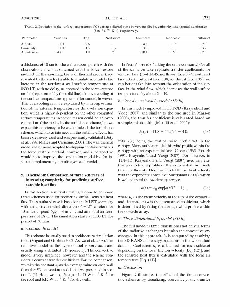
a thickness of 10 cm for the wall and compare it with the
observations and that obtained with the force–restore
method. In the morning, the wall thermal model (rep-
resented by the circles) is able to simulate accurately the
increase in the northwest wall surface temperature at
0600 LT, with no delay, as opposed to the force–restore
model (represented by the solid line). An overcooling of
the surface temperature appears after sunset, however.
This overcooling may be explained by a wrong estima-
tion of the internal temperature by the evolution equa-
tion, which is highly dependent on the other computed
surface temperatures. Another reason could be an over-
estimation of the mixing by the turbulence scheme, but we
expect this deficiency to be weak. Indeed, the turbulence
scheme, which takes into account the stability effects, has
been extensively used and was previously validated (Buty
et al. 1988; Milliez and Carissimo 2008). The wall thermal
model seems more adapted to shipping containers than is
the force–restore method, however, and a perspective
would be to improve the conduction model by, for in-
stance, implementing a multilayer wall model.
5. Discussion: Comparison of three schemes ofincreasing complexity for predicting surfacesensible heat flux
In this section, sensitivity testing is done to compare
three schemes used for predicting surface sensible heat
flux. The simulated case is based on the MUST geometry
with an upstream wind direction of 2458, a reference
10-m wind speed Uref 5 4 m s21, and an initial air tem-
perature of 188C. The simulation starts at 1200 LT for
period of 30 min.
a. Constant hf model
This scheme is usually used in architecture simulation
tools (Miguet and Groleau 2002; Asawa et al. 2008). The
radiative model in this type of tool is very accurate,
usually using a detailed 3D geometry. The convective
model is very simplified, however, and the scheme con-
siders a constant transfer coefficient. For the comparison,
we take the constant hf as the average value on each wall
from the 3D convection model that we presented in sec-
tion 2b(5). Here, we take hf equal 14.45 W m22 K21 for
the roof and 6.12 W m22 K21 for the walls.
In fact, if instead of taking the same constant hf for all
of the walls, we take separate transfer coefficients for
each surface (roof 14.45; northwest face 3.94; southeast
face 10.78; northeast face 1.38; southwest face 8.35), we
can better take into account the orientation of the sur-
face in the wind flow, which decreases the wall surface
temperatures by about 2–4 K.
b. One-dimensional hf model (1D hf)
In this model employed in TUF-3D (Krayenhoff and
Voogt 2007) and similar to the one used in Masson
(2000), the transfer coefficient is calculated based on
a simple relationship (Martilli et al. 2002):
hf (z) 5 11:8 1 4:2u(z) 2 4:0, (13)
with u(z) being the vertical wind profile within the
canopy. Many authors model this wind profile within the
canopy with an exponential law (Cionco 1965; Rotach
1995; Krayenhoff and Voogt 2007). For instance, in
TUF-3D, Krayenhoff and Voogt (2007) used an itera-
tive way to find a profile of the exponential form with
three coefficients. Here, we model the vertical velocity
with the exponential profile of Macdonald (2000), which
is well adapted to low-density arrays:
u(z) 5 uH exp[a(z/H 2 1)], (14)
where uH is the mean velocity at the top of the obstacles
and the constant a is the attenuation coefficient, which
is determined by fitting the average wind profile within
the obstacle array.
c. Three-dimensional hf model (3D hf)
The full model is three dimensional not only in terms
of the radiative exchanges but also the convective ex-
changes. In this approach, hf is computed by resolving
the 3D RANS and energy equations in the whole fluid
domain. Coefficient hf is calculated for each subfacet
depending on the local friction velocity [Eq. (12)], and
the sensible heat flux is calculated with the local air
temperature [Eq. (11)].
d. Discussion
Figure 9 illustrates the effect of the three convec-
tive schemes by visualizing, successively, the transfer
TABLE 2. Deviation of the surface temperatures (8C) during a diurnal cycle by varying albedo, emissivity, and thermal admittance
(J m22 s20.5 K21), respectively.
Parameter Variation Top Northwest Southeast Northeast Southwest
Albedo 10.1 22.6 21 24.5 21.5 22.3
Emissivity 10.15 21.3 21.2 23.5 21 23.2
Admittance 2400 11.8 12 110.1 12.6 12.5
AUGUST 2011 Q U E T A L . 1721

coefficient, the sensible heat flux, and the surface tem-
perature. The three convective schemes show a differ-
ence of the sensible flux of approximately 100–240
W m22 for the southeast face and northeast face. With
the constant hf model, the surface temperatures are
more homogeneous than in the other two cases. In the
MUST configuration, the building array is not dense,
and therefore the effects of the shadow and the multi-
reflections are small. That is the reason why the tem-
peratures in the constant hf approach show little
difference within each wall. With the 1D hf model, we
can obviously see the 1D inhomogeneity of the surface
temperatures, which is linked to the exponential law
wind profile. The 3D hf model results show the 3D in-
homogeneity of the surface temperatures, linked to the
inhomogeneity of the 3D wind. On the same face with
the same material, we can have a difference of tem-
perature of about 4 K. These results demonstrate the
effects of realistically computing the convection fluxes
on the surface temperature in the urban areas. Note
that in the comparison of the three convective schemes
we change only the transfer coefficient and not the air
temperature (which is computed for each grid cell of
the fluid domain in three dimensions). A simple air tem-
perature model could lead to additional differences.
6. Conclusions and perspectives
New atmospheric radiative and thermal schemes were
implemented in the atmospheric module of the three-
dimensional CFD code known as Code_Saturne. The
purpose of this paper was to study in detail the coupling
between the radiative scheme and the 3D dynamical
model. The model was evaluated with the field mea-
surements from an idealized urban area, the MUST
experiment. The coupled model is able to reproduce the
evolution of the surface temperatures for different sides
of a container within the MUST canopy during a diurnal
cycle despite a delay in warming for the northwest and
southwest faces at sunrise. The simulations also showed
a significant impact of the convective flux on the surface
temperatures.
Because the thermal information available in the
MUST field is insufficient, sensitivity studies were per-
formed that emphasized the dependence of the model
on the parameters describing the building: the properties
of the material. In addition, the internal building tem-
perature shows great importance because the buildings
are made of metal.
We compared two ways of computing the surface
temperature: the force–restore method and a wall ther-
mal model. Because the force–restore method may be
more suited for insulated buildings with a near-constant
internal temperature (which is not very representative
of the MUST containers), we have also tested a one-
layer wall model. Using an appropriate evolution equa-
tion for the interior buildings, the force–restore shows
FIG. 9. Comparison of three convective models with visualization
of the southeast and northeast walls at 1230 LT: (a) transfer co-
efficient hf (W m22 K21), (b) sensible heat flux QH (W m2),
(c) surface temperature T (K). Label 1 indicates the constant hf
model, label 2 is for the 1D hf model, and label 3 represents the 3D
hf model.
1722 J O U R N A L O F A P P L I E D M E T E O R O L O G Y A N D C L I M A T O L O G Y VOLUME 50

good results during the afternoon. It induces a delay in
warming at sunset, however, and for the northwest wall
a delay in cooling, because of the thermal inertia in-
herent to the method. The one-layer wall thermal model
we tested also show some weakness, since it can re-
produce the diurnal cycle of the different surface tem-
perature only with a very low thermal conductivity.
Nevertheless, it seems more adapted to model shipping
containers than is the force–restore method. One pro-
posed improvement is to implement a multilayer 1D
thermal model for the walls, as in Masson (2000) or
Krayenhoff and Voogt (2007), which may be more ad-
equate for such surfaces. In fact, shipping-container
surface temperatures appear difficult to predict with
classical urban models, which for instance do not take
into account the conduction between the walls, which
can be neglected for real buildings but should not be for
metal containers, and a 3D conduction wall model may
in this case be necessary.
We also compared our 3D modeling approach to es-
timate the convective exchanges at the surface (which
consists of solving the 3D RANS equations in the whole
fluid domain) with two modeling approaches found in
the literature: the first approach consists in using a con-
stant heat transfer coefficient, and the second approach
is to use a 1D equation based on a vertical wind profile
within the canopy. The comparisons are made in terms
of the convective transfer coefficients, sensible heat
fluxes, and surface temperatures. The three schemes give
values of the same order of magnitude for the average
surface temperature; nevertheless, only the 3D approach
can reproduce the inhomogeneous effect on the wind
on a surface: the difference of the same wall can
reach 4 K.
The simulation of realistic atmospheric conditions in
the urban areas made possible by this work can be used
for various applications. A first example is to study
pollutant dispersal in a low-wind case. A good descrip-
tion of the heat transfer is essential to describe the
convective movement of the air in the streets and is
very important for air pollution investigations. A second
example is the energy balance of buildings. Estimating
the convection fluxes in simple models can keep the
computing time low and has application in mesoscale
studies; nevertheless, at microscale, it can lead to mis-
leading values in the estimation of the energy loss from
the buildings to the atmosphere. In this case, a good
prediction of the convective flux can be helpful to the
management of the energy consumption and a useful
tool in building design. The simulations’ results show a
significant difference of the parameterizations between
taking a simple convection model and describing the
physical processes in a realistic way, coupling the 3D
dynamics and the radiative processes. The simulations
point out the larger difference in surface temperatures at
different locations on the same wall.
This study is the first step to validate our dynamic–
radiative coupling model. This 3D modeling inves-
tigation can bring more detailed information both on
radiative and convective fluxes in very local-scale stud-
ies. In the MUST case, however, the urban area is ide-
alized. At microscales, small irregularities can break the
repeated flow patterns found in a regular array of con-
tainers with identical shape. In addition, uncertainties
associated with the thickness and the properties of the
material of the container wall limit our ability to vali-
date the results. There are also still challenges for mod-
eling in this area. The comparison of three different
modeling approaches to estimate the convective ex-
changes at the surface could be compared with observa-
tions if thermal images are available. That is the reason
why we will evaluate the coupled dynamic–radiative
model on a district of a real urban area with the Canopy
and Aerosol Particles Interactions in Toulouse Urban
Layer (CAPITOUL) experiment (in the city of Toulouse,
France) (Masson et al. 2008; Lagouarde et al. 2010) for
which thermal infrared images are available.
Another perspective of this work is to apply the 3D
radiative scheme to nontransparent media. Indeed, in
many urban applications, the atmosphere between the
boundaries can be considered to be transparent and
nondiffusive. Nevertheless, when studying smoke dis-
persion or fog formation and dissipation, absorption and
diffusion play an important role. Absorption can already
be taken into account by our scheme, and one important
perspective of this work is to study radiation in 3D non-
transparent media and add the diffusion term in the res-
olution of the radiative transfer equation.
Acknowledgments. The authors thank the Defense
Threat Reduction Agency (DTRA) for providing access
to the MUST data.
REFERENCES
Archambeau, F., N. Mechitoua, and M. Sakiz, 2003: Code_Saturne:
A finite volume code for the computation of turbulent in-
compressible flows—Industrial applications. Int. J. Finite Vol., 1,1–62.
Arnfield, A. J., 2003: Two decades of urban climate research: A
review of turbulence, exchanges of energy and water, and the
urban heat island. Int. J. Climatol., 23, 1–26.
Asawa, T., A. Hoyano, and K. Nakaohkubo, 2008: Thermal design
tool for outdoor space based on a numerical simulation system
using 3D-CAD. Build. Environ., 43, 2112–2123.
Biltoft, C. A., 2001: Customer report for Mock Urban Setting Test.
West Desert Test Center, U.S. Army Dugway Proving Ground,
DPG Doc. WDTC-FR-01-121, 58 pp.
AUGUST 2011 Q U E T A L . 1723

Brook, D. R., N. V. Beck, C. M. Clem, D. C. Strickland, I. H.
Griffits, D. J. Hall, R. D. Kingdon, and J. M. Hargrave, 2002:
Validation of the Urban Dispersion Model (UDM). Proc.
Eighth Int. Conf. on Harmonisation within Atmospheric Dis-
persion Modelling for Regulatory Purposes, Sofia, Bulgaria, Na-
tional Institute of Meteorology and Hydrology of Bulgaria, 8–12.
Buty, D., J. Y. Caneill, and B. Carissimo, 1988: Simulation nu-
merique de la couche limite atmospherique en terrain com-
plexe au moyen d’un modele mesometeorologique non
hydrostatique: Le code mercure (Numerical simulation of the
atmospheric boundary layer in complex terrain by means of
a nonhydrostatic model: The Mercury code). J. Theor. Appl.
Mech., 7, 35–62.
Camelli, F. E., R. Lohner, and S. R. Hanna, 2005: VLES study of
MUST experiment. Proc. 43rd AIAA Aerospace Sciences
Meeting and Exhibit, Reno, Nevada, American Institute of
Aeronautics and Astronautics, 1–19.
Cionco, R. M., 1965: A mathematical model for air flow in a vege-
tative canopy. J. Appl. Meteor., 4, 517–522.
Deardorf, J. W., 1978: Efficient prediction of ground surface tem-
perature and moisture with inclusion of a layer of vegetation.
J. Geophys. Res., 83, 1889–1903.
Dupont, S., and P. Mestayer, 2006: Parameterization of the urban
energy budget with the submesoscale soil model. J. Appl.
Meteor. Climatol., 45, 1744–1765.
Eichhorn, J., and M. Balczo, 2008: Flow and dispersal simulations
of the Mock Urban Setting Test. Proc. 12th Int. Conf. on
Harmonisation within Atmospheric Dispersion Modelling for
Regulatory Purposes, Cavtat, Croatia, Meteorological and
Hydrological Service of Croatia, 67–72.
Fiveland, W. A., 1984: Discrete-ordinates solutions of the radiative
transport equation for rectangular enclosure. J. Heat Transfer,
106, 699–706.
Garratt, J. R., 1992: The Atmospheric Boundary Layer. Cambridge
University Press, 316 pp.
Gastellu-Etchegorry, J., 2008: 3D modeling of satellite spectral
images, radiation budget and energy budget of urban land-
scapes. Meteor. Atmos. Phys., 102, 187–207.
——, E. Martin, and F. Gascon, 2004: DART: A 3-D model for
simulating satellite images and surface radiation budget. Int.
J. Remote Sens., 25, 75–96.
Grimmond, C. S. B., and T. R. Oke, 1999: Heat storage in urban
areas: Local-scale observations and evaluation of a simple
model. J. Appl. Meteor., 38, 922–940.
Hanna, S. R., S. Tehranian, B. Carissimo, R. W. Macdonald, and
R. Lohner, 2002: Comparisons of model simulations with ob-
servations of mean flow and turbulence within simple obstacle
arrays. Atmos. Environ., 36, 5067–5079.
Johnson, G. T., T. R. Oke, T. J. Lyons, D. G. Steyn, I. D. Watson,
and J. A. Voogt, 1991: Simulation of surface urban heat islands
under ‘ideal’ conditions at night. Part I: Theory and tests
against field data. Bound.-Layer Meteor., 56, 275–294.
Kanda, M., T. Kawai, M. Kanega, R. Moriwaki, K. Narita, and
A. Hagishima, 2005: A simple energy balance model for reg-
ular building arrays. Bound.-Layer Meteor., 116, 423–443.
Krayenhoff, E. S., and J. A. Voogt, 2007: A microscale three-
dimensional urban energy balance model for studying surface
temperatures. Bound.-Layer Meteor., 123, 433–461.
Lagouarde, J. P., A. Henon, B. Kurz, P. Moreau, M. Irvine, J. Voogt,
and P. Mestayer, 2010: Modelling daytime thermal infrared
directional anisotropy over Toulouse city centre. Remote Sens.
Environ., 114, 87–105.
Lemonsu, A., C. S. B. Grimmond, and V. Masson, 2004: Modelling
the surface energy balance of an old Mediterranean city core.
J. Appl. Meteor., 43, 312–327.
Liu, J., H. M. Shang, and Y. S. Chen, 2000: Development of an
unstructured radiation model applicable for two-dimensional
planar, axisymmetric, and three-dimensional geometries. J. Heat
Transfer, 66, 17–33.
Louis, J., 1979: A parametric model of vertical eddy fluxes in the
atmosphere. Bound.-Layer Meteor., 17, 187–202.
Macdonald, R. W., 2000: Modelling the mean velocity profile in the
urban canopy layer. Bound.-Layer Meteor., 197, 25–45.
Martilli, A., A. Clappier, and M. W. Rotach, 2002: An urban sur-
face exchange parameterisation for mesoscale models. Bound.-
Layer Meteor., 104, 261–304.
Masson, V., 2000: A physically based scheme for the urban energy
budget in atmospheric models. Bound.-Layer Meteor., 94,
357–397.
——, C. S. B. Grimmond, and T. R. Oke, 2002: Evaluation of the
Town Energy Balance (TEB) scheme with direct measure-
ments from dry districts in two cities. J. Appl. Meteor., 41,
1011–1026.
——, and Coauthors, 2008: The Canopy and Aerosol Particles
Interactions in Toulouse Urban Layer (CAPITOUL) experi-
ment. Meteor. Atmos. Phys., 102, 135–157.
Miguet, F., and D. Groleau, 2002: A daylight simulation tool for
urban and architectural spaces—Application to transmitted
direct and diffuse light through glazing. Build. Environ., 37,
833–843.
Milliez, M., 2006: Modelisation micro-meteorologique en milieu
urbain: Dispersion des polluants et prise en compte des effets
radiatifs (Micrometeorological modeling in urban environ-
ment. Dispersion of pollutants and the taking into account of
radiative effects). Ph.D. thesis, Ecole des Ponts ParisTech,
228 pp. [Available online at http://cerea.enpc.fr/fich/these_
milliez.pdf.]
——, and B. Carissimo, 2007: Numerical simulations of pollut-
ant dispersion in an idealized urban area, for differ-
ent meteorological conditions. Bound.-Layer Meteor., 122,
321–342.
——, and ——, 2008: CFD modelling of concentration fluctuations
in an idealized urban area, for different meteorological con-
ditions. Bound.-Layer Meteor., 127, 241–259.
——, L. Musson-Genon, and B. Carissimo, 2006: Validation of
a radiative scheme for CFD modelling of heat transfers be-
tween buildings and flow in urban canopies. Preprints, Sixth
Int. Conf. on Urban Climate, Goteborg, Sweden, International
Association of Urban Climate, 266–269.
Mills, G., 1996: An urban canopy-layer climate model. Theor.
Appl. Climatol., 1997, 229–244.
Oke, T. R., 1987: Boundary Layer Climates. 2nd ed. Routledge,
435 pp.
Rotach, M. W., 1995: Profiles of turbulence statistics in and
above an urban street canyon. Atmos. Environ., 29, 1473–1486.
Truelove, J. S., 1987: Discrete-ordinates solutions of the radiative
transport equation. J. Heat Transfer, 109, 1048–1051.
Yee, E., and C. A. Biltoft, 2004: Concentration fluctuations mea-
surements in a plume dispersing through a regular array of
obstacles. Bound.-Layer Meteor., 111, 363–415.
1724 J O U R N A L O F A P P L I E D M E T E O R O L O G Y A N D C L I M A T O L O G Y VOLUME 50

CHAPTER 4
A comparison of two radiation models:
Code_Saturne and SOLENE
Contents
4.1 Introduction . . . . . . . . . . . . . . . . . . . . . . . . . . . . . . . . . . . . 67
4.2 Description of SOLENE model . . . . . . . . . . . . . . . . . . . . . . . . . . 70
4.2.1 Geometry and mesh. . . . . . . . . . . . . . . . . . . . . . . . . . . . 70
4.2.2 Thermo-radiative model. . . . . . . . . . . . . . . . . . . . . . . . . . 72
4.3 Radiation analyses. . . . . . . . . . . . . . . . . . . . . . . . . . . . . . . . . 74
4.3.1 Set-up for radiation computation. . . . . . . . . . . . . . . . . . . . . . 74
4.3.2 Comparison of direct solar flux. . . . . . . . . . . . . . . . . . . . . . . 75
4.3.3 Comparison of diffuse solar flux. . . . . . . . . . . . . . . . . . . . . . 77
4.3.4 Comparison of long-wave radiation flux. . . . . . . . . . . . . . . . . . 80
4.3.5 Comparison of surface temperatures. . . . . . . . . . . . . . . . . . . . 81
4.4 Conclusions and perspectives. . . . . . . . . . . . . . . . . . . . . . . . . . . 82
4.1 Introduction
In order to more accurately model the physics of an urban canopy, new concepts in surface
modeling have been developed. We have mentioned several canopy models (see Chapter 2

68 Chapter 4. A comparison of two radiation models:Code_Saturne and SOLENE
and 3) which aim to solve the Surface Energy Balance (SEB) fordifferent applications, such
as TEB (Masson, 2000), UCLCM (Mills , 1996), SOLENE (Miguet and Groleau, 2002), 3D-
CAD(Asawa et al., 2008), DART-EB(Gastellu-Etchegorry, 2008), TUF-3D (Krayenhoff and
Voogt, 2007) and SUMM(Kanda et al., 2005). In order to model the radiation exchanges, many
SEB models (e.g.Miguet and Groleau(2002); Asawa et al.(2008); Krayenhoff and Voogt
(2007)) employ the radiosity method. That is, all radiative reflection and emission is assumed
perfectly diffuse without absorption (i.e. Lambertian). The effects of surface morphology
on the radiative exchange between a closed system of surfaces surrounding a non-absorbing
medium are expressed in terms of the view factors or shape factors for the system of surfaces.
Surface morphology affects the radiation balance by altering the magnitude and source of the
radiative flux densities incident on each surface. The view factors or shape factors are required
when applying the radiosity method to an urban street canyonwhich are between two equally
sized, in-line, parallel planes and between two perpendicular planes sharing a common edge
(A1 andA2), as shown in Figure4.1.
Shape factors for the radiative exchange between any two of the canyon surfaces can be
derived from one of these two generic types. In general, the radiation is reflected multiple
times until the remaining unabsorbed radiation is below a user-defined threshold. Short- and
long-wave reflection and absorption are modeled with the same method, but are initialized dif-
ferently to properly account for shading of direct solar, diffuse solar, and for long-wave emitted
from both the sky and the urban surfaces. Each patch requiresan albedo and an emissivity as
input, while outputs for both wavelength ranges include total reflected radiation, total reflected
radiation escaping to the sky, and total absorbed radiationby surfaces.
Since our aim is to model radiative exchange in the ABL (0∼ 200m), for instance, even-
tually with the smoke or fog between the buildings, we chose the Discrete Ordinate Method to
solve the radiative transfer equation in the whole fluid domain forCode_Saturne. This approach
is less precise than the radiosity method to estimate the incoming radiative fluxes on urban sur-
faces, but we can calculate the radiation flux not only on the facets of the urban landscape but
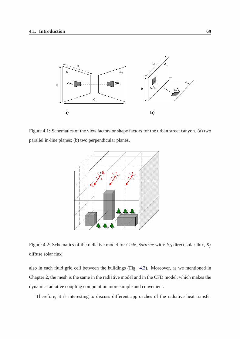
4.1. Introduction 69
Figure 4.1: Schematics of the view factors or shape factors for the urban street canyon. (a) two
parallel in-line planes; (b) two perpendicular planes.
Figure 4.2: Schematics of the radiative model forCode_Saturne with: SD direct solar flux,Sf
diffuse solar flux
also in each fluid grid cell between the buildings (Fig.4.2). Moreover, as we mentioned in
Chapter 2, the mesh is the same in the radiative model and in the CFD model, which makes the
dynamic-radiative coupling computation more simple and convenient.
Therefore, it is interesting to discuss different approaches of the radiative heat transfer
70 Chapter 4. A comparison of two radiation models:Code_Saturne and SOLENE
models. Here we compare the radiative models inCode_Saturne and SOLENE with MUST
experimental data set.
4.2 Description of SOLENE model
Initially designed for simulating sunshine, natural lighting and thermal radiation over build-
ings or urban blocks for architectural projects, SOLENE software is developed by CERMA
laboratory (http://solene.cerma.archi.fr/) and has been applied in many works (e.g.Ringenbach
(2004); Robitu (2005); Hénon(2008); Kurz (2009); Bouyer(2009); Hénon et al.(2011a,b,c)
etc.).
4.2.1 Geometry and mesh
With no particular restriction about the geometry and size,taking into account the urban mor-
phology, SOLENE allows simulating different quantities and phenomena, such as the sunshine
features (lighting and mask), the various components of solar radiation (direct and diffuse flux
incident on each element with multiple reflections between surface features) and thermal in-
frared radiation. With the "contour integration" method (e.g. Soux et al.(2004)) the view
factors method implemented in SOLENE may be rapidly and precisely calculated between
four-sided surfaces of any orientation.
In SOLENE, a geometry is defined by a set of unconnected plane faces, with oriented
normal (in general, outward). Each face is constituted itself one or more plane facets. These
facets as known contour, which are polygons defined by the coordinates of each vertex relative
to the origin, and by the components of the vector normal. Fora same face, the contours
are connected and they correspond to the cell of the computational model. Through the 3D
geometric modeling of urban morphology, SOLENE triangulates the computational object to
a shell mesh. The sky vault is considered as a hemisphere of infinite radius, with the scene
to be simulated located at its center. This hemisphere is meshed with a geodesic triangulation

4.2. Description of SOLENE model 71
of 4n elements (e.g. 1024 is a good compromise between precision and speed in most of the
time (Miguet and Groleau, 2002)). The sky is considered as a source of diffuse energy with a
non-uniform solar radiation or luminance distribution (e.g. in Fig. 4.3). Different atmosphere
and cloud cover conditions are defined by two coefficients, epsilon and delta from a sky model
of Perez et al.(1993). Epsilon is in the range from 1 to 12 which defines the cloud coverage
(more than 6 for clear sky) and delta from 0.01 to 0.6 which defines the opacity linked to the
thickness of the clouds, from highly sombre to very shiny. The information assigned to the cell
is organized as a descriptor file. A descriptor is a set of numerical values assigned to a single
cell. Thus, each parameter describing the scene has an associated description file. In addition,
for the variables over time, we need a description file per time step.
Figure 4.3: Visualization in SOLENE of: a) a dimensionless clear sky hemisphere exhibiting
1024 patches with a radiance distribution at 1500 LST; b) thetriangularized shell meshing
MUST geometry.

72 Chapter 4. A comparison of two radiation models:Code_Saturne and SOLENE
4.2.2 Thermo-radiative model
Net short-wave radiative flux The direct solar radiation is emitted by the sky in the sun
direction while the diffuse solar radiation emission is distributed on all sky facets according to
the sky radiance model. In a given scene, SOLENE starts the computation with view factors,
incident solar flux and inputs the albedo of each facet. From the incident short-wave radiative
flux, the model calculates the total solar flux reflected by thescene and then distribute it to other
facets. The contribution of a facet on others is determined by a progressive refinement method:
we consider the maximal short-wave radiative flux reflected by a facet, then distribute on other
facets and determine the new maximal reflected solar flux and so on. The process continues
until the difference in the distribution of the solar flux reaches a threshold defined by the user
(e.g. 5W) or other convergence criteria (e.g. the number of iterations).
Net long-wave radiative flux In SOLENE, the treatment of the infrared flux is similar to the
solar flux by using the progressive radiosity algorithm. Themodel use an empirical equation
(Monteith and Unsworth, 1990) to estimate the incident infrared flux:
L↓ = 213+5.5Ta, (4.1)
whereL↓ (W m−2) andTa (K) are respectively incoming long-wave radiation flux from the
atmosphere and air temperature.
However, for the long-wave radiative flux, the facets not only absorb and reflect infrared flux
but they also emit. The emission term is determined through the Stefan-Boltzmann lawεσT4s f c
which depends on the surface temperatureTs f c (see Chapter 2 radiative model). SOLENE can
read the atmospheric radiative fluxes and the air temperature meteorological data as input which
is the case in this comparison.
Surface temperature model A multi-layers wall model (one or two layers) is implementedin
the SOLENE to determine temperature, over time, at the surface and inside the wall. Thus, for
single layer wall, the external surface node, with 1/10 of the heat capacity of the wall reflects

4.2. Description of SOLENE model 73
the relatively rapid thermal response of external variations (air, solar and infrared radiation)
while the internal node with 9/10 of the heat capacity plays the inertial role. The two layers
wall is built on the same bases.
As shown in Figure4.4, the conductance (K) and heat capacity (C) are characteristic of
the material related to the thickness of the layer (e). For the interior nodes of the layers, we
consider that the conductance is identical on each side:
K1 = 2λ1/e1; K2 = 2λ2/e2, (4.2)
whereK (W K−1 m−2), λ (W K−1 m−1) ande(m) are respectively the conductance, the thermal
conductivity and the thickness of the layer associated to the first node or second node.
The heat capacity is evaluated as:
C1 = ρ1Cm1e1; C2 = ρ2Cm2e2, (4.3)
whereC (J K−1 m−2), ρ (kgm−3) andCm (J K−1 kg−1) are respectively the heat capacity, the
density and the mass-specific heat capacity associated to the node 1 or 2.
Hence, the thermal budget of each node is computed as follows(Antoine and Groleau,
1998; Hénon, 2008) for the external nodeselinking to external surface temperatureTse (K):
0.1C1dTse
dt+K1(Tse−Tn1)+QH +L∗ = S∗, (4.4)
wheredt (s) the time step,Tn1 (K) the temperature at noden1, QH (W m2) the sensible heat
flux estimated with equation1.7, L∗ (W m2) andS∗ (W m2) are respectively the net long-wave
and short-wave radiation flux.
For the nodes1 linking to the surface temperatureTs1 (K):
0.9C1dTn1
dt+K1(Tn1−Tse)+K1(Tn1−Ts1) = 0, (4.5)
for the noden2 linking to the internal temperatureTn2 (K):
C2dTn2
dt+K2(Tn2−Ts1)+K2(Tn2−Ts2) = 0, (4.6)

74 Chapter 4. A comparison of two radiation models:Code_Saturne and SOLENE
for the nodes2 linking to the wall temperatureTs2 (K), not to the ground (same as in
Code_Saturne, a constant temperature applied to deep soil)
K2(Ts2−Tn2)+hi(Ts2−Tint) = 0, (4.7)
wherehi (W m−2K−1) is a global internal building heat transfer coefficient andTint (K) the
internal building temperature.
Figure 4.4: Schematic representation of the energy exchanges at an urban surface for SOLENE
simulation, afterAntoine and Groleau(1998). Ki andCi represent respectively the conductance
and heat capacity.
4.3 Radiation analyses
4.3.1 Set-up for radiation computation
The simulations are performed with SOLENE version 1.82. The computational effort in time
and memory is not comparable. Because the two models are developed with different operating
systems (Windows for SOLENE with sequential computing, Linux forCode_Saturne with par-
allel computing). Since no CFD quality criteria needs to be respected for the mesh in SOLENE,
we reduced the horizontal size from MUST full radiative-dynamic coupling validation to save
computational time. A standard clear sky model is created with 1024 elements for the SOLENE
simulations. We set a 15mn radiative time step both in SOLENE andCode_Saturne models.

4.3. Radiation analyses 75
Furthermore, when we take into account the multi-refections, 5 iterations is considered for con-
sistency in both models. Based on MUST full dynamic-radiative coupling validation case (see
Chapter 3, Table 1), we summarize the main parameters used inthe simulation for the compari-
son in Table4.1. We keep in mind that all the following comparisons are for the center building
in the domain.
4.3.2 Comparison of direct solar flux
We start with the comparison of direct solar flux before and after multi-reflection by the urban
canopy. Through Figure4.5a, 4.5b, we find that the two models agree quite well with each
other. The estimation of the direct solar flux is slightly higher (by less than 10%) for the
SOLENE model with and without multi-reflection. These relatively slight visible differences
appear only at the south wall (SE and SW faces) and roof which are the most exposed to the
sun during the daytime. Moreover, it seems that SOLENE modelhas a small delay on sunrise.
This may be due to the difference on the accuracy of estimating the time of sunrise and the
precision of the specified latitude.
0 2 4 6 8 10 12 14 16 18 20 22Local time (h)
0
100
200
300
400
500
600
700
800
Rad
iatio
n flu
x de
nsity
(W
/ m
²)
Top(Code_Saturne)NW (Code_Saturne)SE (Code_Saturne)NE (Code_Saturne)SW (Code_Saturne)Top(SOLENE)NW (SOLENE)SE (SOLENE)NE (SOLENE)SW (SOLENE)
a)
0 2 4 6 8 10 12 14 16 18 20 22Local time (h)
0
100
200
300
400
500
600
700
800
Rad
iatio
n flu
x de
nsity
(W
/ m
²)
Top(Code_Saturne)NW (Code_Saturne)SE (Code_Saturne)NE (Code_Saturne)SW (Code_Saturne)Top(SOLENE)NW (SOLENE)SE (SOLENE)NE (SOLENE)SW (SOLENE)
b)
Figure 4.5: Comparison for the central container of the MUSTfield experiment of direct solar
radiation flux on roof (top), N-W, S-E, N-E and S-W walls during a diurnal cycle between
Code_Saturne (Straight line) and SOLENE (Dashed line): a) incident direct solar flux; b) direct
solar flux after multi-reflections.
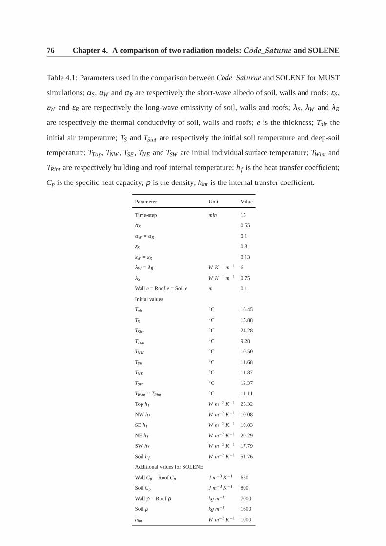
76 Chapter 4. A comparison of two radiation models:Code_Saturne and SOLENE
Table 4.1: Parameters used in the comparison betweenCode_Saturne and SOLENE for MUST
simulations;αS, αW andαR are respectively the short-wave albedo of soil, walls and roofs; εS,
εW andεR are respectively the long-wave emissivity of soil, walls and roofs; λS, λW andλR
are respectively the thermal conductivity of soil, walls and roofs; e is the thickness;Tair the
initial air temperature;TS andTSint are respectively the initial soil temperature and deep-soil
temperature;TTop, TNW, TSE, TNE andTSW are initial individual surface temperature;TWint and
TRint are respectively building and roof internal temperature;hf is the heat transfer coefficient;
Cp is the specific heat capacity;ρ is the density;hint is the internal transfer coefficient.
Parameter Unit Value
Time-step min 15
αS 0.55
αW = αR 0.1
εS 0.8
εW = εR 0.13
λW = λR W K−1 m−1 6
λS W K−1 m−1 0.75
Wall e= Roofe = Soil e m 0.1
Initial values
TairC 16.45
TSC 15.88
TSintC 24.28
TTopC 9.28
TNWC 10.50
TSEC 11.68
TNEC 11.87
TSWC 12.37
TWint = TRintC 11.11
Top hf W m−2 K−1 25.32
NW hf W m−2 K−1 10.08
SEhf W m−2 K−1 10.83
NE hf W m−2 K−1 20.29
SW hf W m−2 K−1 17.79
Soil hf W m−2 K−1 51.76
Additional values for SOLENE
Wall Cp = RoofCp J m−3 K−1 650
Soil Cp J m−3 K−1 800
Wall ρ = Roofρ kg m−3 7000
Soil ρ kg m−3 1600
hint W m−2 K−1 1000

4.3. Radiation analyses 77
4.3.3 Comparison of diffuse solar flux
With regard to the diffuse solar flux the differences betweenSOLENE andCode_Saturne are
significant (Fig.4.7a), in particular at the four walls, whereCode_Saturne model predicts the
same average diffuse solar flux (superimposed lines in Fig.4.7a). This can be explained by
the fact that the simple clear sky model, Bird Clear Sky model(Bird and Hulstrom, 1981),
implemented inCode_Saturne assumes the homogeneous and isotropic intensity distribution
of diffuse solar flux at inlet boundaries (see Chapter 2 section2.3.2.c).
Figure 4.6: Schematics of the procedure to impose the SOLENEvalues of diffuse solar flux
as boundary conditions inCode_Saturne. The verification box is used to check the calculated
values inCode_Saturne.
In order to analyze the difference further we have introduced the SOLENE inhomogeneous
diffuse solar flux as the boundary conditions inCode_Saturne, using the following procedure
(Fig. 4.6):
1. In SOLENE, we create a "rectangular building" as large as the computational domain of
Code_Saturne (box with dashed lines in Fig.4.6) and afterwards, compute the average
diffuse solar flux for each face of this large building using SOLENE.
78 Chapter 4. A comparison of two radiation models:Code_Saturne and SOLENE
2. Make a second large "rectangular building" which is just alittle smaller (−1m) than the
previous one which will be used as verification box for both SOLENE andCode_Saturne
(box with full lines in Fig. 4.6). Use the average diffuse flux value from the pre-
vious step as inlet boundary conditions for each boundary ofthe computational do-
main inCode_Saturne. Compute the diffuse flux for second building in SOLENE and
Code_Saturne (box with full lines in Fig. 4.6). Compare the results to check if the
boundary condition is correctly set inCode_Saturne (Fig. 4.7b).
3. Apply the diffuse flux value from SOLENE to the MUST reference geometry in
Code_Saturne (small blue boxes in Fig.4.6) and compare the values for the container
walls (Fig.4.7(c)).
As shown in Figure4.7b, taking the average diffuse solar flux value from SOLENE as inlet
boundary condition gives a very good agreement between SOLENE andCode_Saturne. How-
ever, the comparison for the container walls is not enough assatisfactory as expected. As shown
in Figure4.7c, the diffuse flux of each side of the wall reproduced byCode_Saturne differ a lot.
Only the roof matches well, but all the sides wall exhibit over or underestimation. The problem
can be explained by recalling that the Discrete Ordinates Method has a quite limited angular
at any discretization resolution (32 or 128 directions). Since the incident diffuse radiation is
restricted to propagate in a finite number of directions withan angular sector width from the
boundary into the domain, they may not all reach the verticalbuilding surfaces but somewhere
else in the domain, except for the roof which is a horizontal surface and at the highest level
can receive the diffuse flux from all the directions. This is also proved by the result shown in
Figure4.7b where the distance from boundary to building surface is very short. Since the direct
solar flux is unidirectional, the distance between the building and the boundary does not have
the same influence on the results inCode_Saturne (Fig. 4.5).
Nevertheless, using the diffuse flux value from SOLENE inCode_Saturne still shows an
improvement. Moreover, in clear sky condition, compared tothe direct solar flux, the diffuse
flux plays a minor role in the surface energy balance.

4.3. Radiation analyses 79
0 2 4 6 8 10 12 14 16 18 20 22Local time (h)
0
20
40
60
80
100
120
140
Rad
iatio
n flu
x de
nsity
(W
/ m
²)
Top(Code_Saturne)NW (Code_Saturne)SE (Code_Saturne)NE (Code_Saturne)SW (Code_Saturne)Top(SOLENE)NW (SOLENE)SE (SOLENE)NE (SOLENE)SW (SOLENE)
a)* for MUST container
0 2 4 6 8 10 12 14 16 18 20 22Local time (h)
0
20
40
60
80
100
120
140
Rad
iatio
n flu
x de
nsity
(W
/ m
²)
Top(Code_Saturne)NW (Code_Saturne)SE (Code_Saturne)NE (Code_Saturne)SW (Code_Saturne)Top(SOLENE)NW (SOLENE)SE (SOLENE)NE (SOLENE)SW (SOLENE)
b)* for verification box
0 2 4 6 8 10 12 14 16 18 20 22Local time (h)
0
20
40
60
80
100
120
140
Rad
iatio
n flu
x de
nsity
(W
/ m
²)
Top(Code_Saturne)NW (Code_Saturne)SE (Code_Saturne)NE (Code_Saturne)SW (Code_Saturne)Top(SOLENE)NW (SOLENE)SE (SOLENE)NE (SOLENE)SW (SOLENE)
c)* for MUST container
Figure 4.7: Comparison between SOLENE andCode_Saturne for incident diffuse solar flux:
a) for the container walls with Bird Clear Sky model inCode_Saturne; b) using the SOLENE
diffuse flux values from SOLENE model as boundary conditionsto theCode_Saturne for walls
of the verification box (see Fig.4.6); c) for the container walls with SOLENE boundary condi-
tions applied inCode_Saturne.

80 Chapter 4. A comparison of two radiation models:Code_Saturne and SOLENE
4.3.4 Comparison of long-wave radiation flux
Since the observation of the incident long-wave radiation flux is available in the MUST data,
we use it as sky boundary conditions for bothCode_Saturne and SOLENE. Here we compare
only the output of the average incident long-wave radiationflux at each face of the building
for the two models. Figure4.8indicates that the prediction of the incident long-wave radiation
agrees very well with two models (black dashed line and blackstraight line is superimposed.).
The average incident long-wave radiation flux on the four sides of building wall exhibits an
isotropic behavior (straight/dashed lines are all superimposed). Unlike the distribution of the
diffuse solar flux which depends on the position of the sun, the distribution of the incident
infrared flux at each boundary is isotropic. Therefore the symmetric building geometry makes
each wall receive the same quantity of the average infrared flux. Thus,Code_Saturne calculates
the incident infrared radiation as well as SOLENE.
0 2 4 6 8 10 12 14 16 18 20 22Local time (h)
100
150
200
250
300
350
400
Rad
iatio
n flu
x de
nsity
(W
/ m
²)
Top(Code_Saturne)NW (Code_Saturne)SE (Code_Saturne)NE (Code_Saturne)SW (Code_Saturne)Top(SOLENE)NW (SOLENE)SE (SOLENE)NE (SOLENE)SW (SOLENE)
Figure 4.8: Same as Fig.4.5but for incident long-wave radiation flux.

4.3. Radiation analyses 81
4.3.5 Comparison of surface temperatures
Up to now, we have compared the atmospheric radiation flux term by term. Since the primary
aim of our radiative model is to calculate the exterior surface temperatures of the facets, finally
we discuss the prediction of the surface temperatures by thetwo models. Focusing on radiative
aspects, the computation of the sensible heat flux is strongly idealized for this test. The sim-
ulations are based on a given constanthf for each face of the buildings and ground every two
hours. The constanthf values are obtained by averaging the result of our dynamic-radiative
full coupling model (see Chapter 3). Thus, no conservation equations for mass, momentum
and energy are solved and therefore the influence of a model other than the radiation model can
be excluded. We use the wall thermal model fromCode_Saturne (see Chapter 2) and consider
one-layer wall from SOLENE to calculate the surface temperature. The air temperature and in-
cident long-wave radiation are directly imposed from meteorological data. Since the influence
of the internal building temperature on the external surface temperature is quite important in the
MUST case (see Chapter 3), we update the diurnal variation ofthe interior temperature every
half hour. Furthermore, we estimate the values for the specific heat capacityCp and the density
ρ in SOLENE (Tab.4.1) which are close to the MUST experimental field. In the SOLENE
models the internal building energy balance, and the internal transfer coefficienthint must to be
set. In order to keep an equivalent heating configuration, after testing some values in SOLENE,
we find that by taking a high value ofhint is easier to getTs f c∼ Tint . Thus,hint is set to 1000.
Figure 4.9 displays the time evolution of modeled surface temperatures using the
Code_Saturne and SOLENE, and the observation data as reference. Overall,the mean sur-
face temperatures is rather well reproduced by both models.The diurnal cycle is also well
simulated and the variability of the two models and the observations are comparable. On the
other hand, this good result is also consistent with the ability of our full dynamic-radiative
coupling to estimate good averagehf values.
The surface temperature is better simulated byCode_Saturne with a bias smaller than 5C.
This is may be due to a lack of information on some thermal properties in the experiment. The

82 Chapter 4. A comparison of two radiation models:Code_Saturne and SOLENE
estimated parameters in the simulation might be better adapted for the one-layer wall thermal
model inCode_Saturne. Additionally unknown parameters (Cp andρ) used in SOLENE may
lead to more uncertainties. However, it can be seen that SOLENE has a slight tendency to
predict lower wall temperature than those observed in the morning. This underestimation is
more accentuated for SE (Fig.4.9b) and NE wall (Fig. 4.9c). Furthermore, SOLENE also
overestimate the surface temperatures starting from the middle of the day. This behavior of
the model is probably associated with a strong contributionof the thermal inertia leading to
a delay in warming with storage in the morning then heat releases from the middle of the
day. In addition, bothCode_Saturne and SOLENE can produce a visualization of the 3D field.
For instance, the distribution of the surface temperaturesat 1000 LST is pictured in Figure
4.10. The visualization of the building temperatures is consistent with the above discussion.
Moreover, the ground temperature reproduced by SOLENE (Fig. 4.10b) is higher than by
Code_Saturne (Fig. 4.10b) (∼> 5C). Difference with the MUST shipping container surface
temperatures are highly dependent on the evolution of the internal temperature, the diurnal
variation of the deep ground temperature being insignificant. So one reason for the ground to
appear warmer in SOLENE maybe the estimation of the value ofCp andρ for the soil. By using
an one-layer wall scheme, they may be sensitive to the solution of the ground temperature in
SOLENE for this particular case.
4.4 Conclusions and perspectives
In this study, we have compared the atmospheric radiation fluxes and the container walls surface
temperature simulated byCode_Saturne and SOLENE models with the MUST experimental
data set. It has been found that both two models give similar mean daily cycle of radiation
fluxes. For the direct solar flux and incident infrared flux,Code_Saturne is in very good cor-
respondence with the SOLENE model. The prediction of the diffuse solar flux by the Discrete
Ordinate Method ofCode_Saturne is poorer, due to an assumption of isotropy uniform sky
and the different characteristics of the numerical method.Concerning the surface temperature,

4.4. Conclusions and perspectives 83
0 2 4 6 8 10 12 14 16 18 20 22Local time (h)
0
10
20
30
40
50
Sur
face
tem
pera
ture
(°C
)
Top(obs.)Top(Code_Saturne)Top(SOLENE)
a)
0 2 4 6 8 10 12 14 16 18 20 22Local time (h)
0
10
20
30
40
50
60
Sur
face
tem
pera
ture
(°C
)
NW (obs.)SE (obs.)NW (Code_Saturne)SE (Code_Saturne)NW (SOLENE)SE (SOLENE)
b)
0 2 4 6 8 10 12 14 16 18 20 22Local time (h)
0
10
20
30
40
50
60
Sur
face
tem
pera
ture
(°C
)
NE (obs.)SW (obs.)NE (Code_Saturne)SW (Code_Saturne)NE (SOLENE)SW (SOLENE)
c)
Figure 4.9: Evolution of surface temperature of different faces of the central container in MUST
field experiment during a diurnal cycle (cross symbol: Measurements; Straight line: Simulation
with Code_Saturne; Dashed line: Simulation with SOLENE).

84 Chapter 4. A comparison of two radiation models:Code_Saturne and SOLENE
Figure 4.10: Comparison of two radiative models with visualization of surface temperatures
(Ts f c) (C) of ground, roof, SE and NE wall at 1000 LST: a)Code_Saturne; b) SOLENE.

4.4. Conclusions and perspectives 85
with imposed heat transfer coefficients, the ensemble average diurnal cycle of the surface tem-
perature of different building sides is well reproduced by both models. Incertitude related to
additional thermal parameters,Cp andρ , is more pronounced for the ground temperature in
SOLENE. Both of them have facility to the visualization of the 3D field. They can be useful
tools for simulating the outdoor thermal environment.
Further, only one-layer wall thermal model is tested here. Using a multi-layer scheme and
includingCp andρ with more detailed information on properties of the material may be appro-
priate to compare SOLENE andCode_Saturne. In case where the diffuse flux data is not avail-
able or in cloudy sky weather conditions, calculating the diffuse flux value from SOLENE with
a domain size box then set as inlet boundary conditions lead to improvements inCode_Saturne
results. Conversely, using a CFD code to more accurately model thehf is helpful to SOLENE
for predicting the sensible heat flux under moderate wind speed condition.


CHAPTER 5
Numerical study of the thermal effects of
buildings on low-speed airflow taking into
account 3D atmospheric radiation in
urban canopy: paper submitted to Journal
of Wind Engineering & Industrial
Aerodynamics
In the two previous chapters, we discussed the impact of the convective flux on the surface
temperatures by modeling a detailed wind field. Then, on the radiation aspect, we discussed
the performance of the radiative model in comparison to SOLENE model. In this submitted
paper, in order to improve the model, we extend the work of Chapter 3 and 4. We present
different numerical simulations for low wind speed and higher building density than in MUST,
varying the thermal exchange model and analyzing the differences. On one hand, this assess
the thermal impact on the flow field in different conditions. On the other hand, it illustrates the
use of the 3D radiative scheme.

Numerical study of the thermal effects of buildings onlow-speed airflow taking into account 3D atmospheric
radiation in urban canopy
Yongfeng QU1,∗, Maya MILLIEZ, Luc MUSSON-GENON and BertrandCARISSIMO
CEREA, 6-8 avenue Blaise Pascal, 77455 Champs-sur-Marne, France
Abstract
A three-dimensional atmospheric radiative model which enables to evaluate the
thermal-radiative transfers in the lower atmosphere was implemented in the at-
mospheric module of a Computational Fluid Dynamics code. This model can
study the thermal effects of buildings on the local atmospheric flow with a cou-
pled dynamic-radiative model. Previously, we have validated this approach by
comparison with several surface wall temperatures from theMock Urban Set-
ting Test experiment. This paper presents idealized simulations with a lower wind
speed and a higher building density and discusses the impactof albedo (dark/white
walls). In order to further analyze the contribution of the 3D radiative transfers,
a comparison of the thermal impact on the airflow under different thermal con-
ditions for the ground and the walls is made: no heating, imposed temperatures
and 3D radiative transfer heating. The results show that taking into account the
∗Corresponding author. Tel. +33 130877217Email address: [email protected] (Yongfeng QU)
1CEREA Teaching and Research Center in Atmospheric Environment, (Ecole des Ponts Paris-Tech / EDF R&D)
Preprint submitted to J. Wind Eng. Ind. Aerodyn. September 7, 2011

thermal stratification has a significant influence on the windfield. The difference
between the imposed temperatures case and the 3D radiative transfer case can also
be important. Furthermore, the influence of the different radiative transfer condi-
tions and parameters are also discussed: a 0900 LST sun position with an albedo
of 0.1 for the building walls, a 0900 LST sun position with an increased value of
the albedo (0.6) and a 1600 LST sun position with an albedo of 0.1 are compared.
Keywords: Thermal transfer, 3D atmospheric radiation, Computational Fluid
Dynamics, Urban canopy
1. Introduction
The influence, on the airflow pattern, of the incident atmospheric radiation on
the canyon walls and ground surfaces under conditions of lowwind speed can
be important and should not be neglected in pollutant dispersion or urban de-
sign studies. Solar heating of the building walls and the ground during the day
warms the air near the wall or above the ground, which can cause strong ther-
mally induced air motion. This thermal effects on the airflow, including building
geometry and architecture as well as street canyon dimensions, have been mainly
studied with wind-tunnel experiments (Uehara et al., 2000;Kovar-Panskus et al.,
2002; Richards et al., 2006) and numerical models (Sini et al., 1996; Kim and
Baik, 2001; Louka et al., 2001; Xie et al., 2007) and fewer with full-scale or near
full-scale experiments (Louka et al., 2001; Kanda, 2006; Niachou et al., 2008).
In general, field and wind-tunnel experimentalists stress the technical difficulties
in controlling air and surface temperatures and various airor surface tempera-
tures gradients. Moreover, in order to obtain significant thermal effects and re-
spect the similarity with a real building, usually a very high surface temperature
2

(100−400C) has to be applied in wind-tunnel experiments (Uehara et al., 2000;
Kovar-Panskus et al., 2002; Richards et al., 2006).
To overcome this limitation, numerical studies were performed. Sini et al.
(1996) first numerically showed that the thermal forcing could markedly influence
the air motions and the wind structure. Later, Kim and Baik (2001) simulated the
flow in an urban street canyon with various aspect ratios and with street bottom
heating using a two-dimensional (2D, hereafter) Computational Fluid Dynamics
(CFD, hereafter) model with a k-ε turbulence closure. Kovar-Panskus et al. (2002)
identified the differences in the airflow regimes between thecases with and with-
out wall heating. Xie et al. (2007) investigated the influence of the multi-surface
heating configuration on the flow field and pollutant transport problems with the
wind-tunnel experiment of Uehara et al. (2000).
However, most of previous research works considered a 2D computational do-
main and assumed idealized sunlit wall configurations (uniform sunlight on one
surface of the canyon and no sunlight on any other solid surfaces) without includ-
ing a realistic radiative model. Further research work is therefore necessary to
improve our knowledge about the thermal effects on local atmospheric environ-
ment. On the basis of this background, the aim of this work is to perform three-
dimensional (3D, hereafter) numerical simulations in order to evaluate the effects
of non-uniform wall-heating on the airflow pattern using a 3Dradiative model de-
veloped in the CFD codeCode Saturne which is adapted to complex geometry.
Milliez (2006) first evaluated the model with idealized cases, using a constant 3D
wind field. Then, Qu et al. (2011) compared this model with measurements of
surface temperature for different wall orientation in the Mock Urban Setting Test
(MUST, hereafter) field campaign (Yee and Biltoft, 2004; Milliez and Carissimo,
3

2007). They have also discussed the influence on the surface temperatures of the
internal building temperature and the wall thermal modeling, and compared the
3D modeling of the convective exchanges to simpler approaches used in other
models. In this paper, we extend the work of Qu et al. (2011) tolower wind speed
and a higher building density than in MUST. First, we briefly describe the model
and discuss the thermal exchange modeling of buildings. Then we present dif-
ferent numerical simulations for low wind speed in this idealized urban area with
a high building density, varying the thermal exchange modeland analyzing the
differences.
2. Equations and Model design
The model used in this study is the open-source CFD codeCode Saturne (Ar-
chambeau et al., 2004) which can handle complex geometry andphysics. Taking
into account the larger scale meteorological conditions and the thermal stratifi-
cation of the atmosphere, the atmospheric module ofCode Saturne, described
in Milliez and Carissimo (2007), uses a detailed representation of the surfaces
allowing a complex 3D spatial representation of wind speed,turbulence, and tem-
perature. The numerical solver employs a finite-volume approach for co-located
variables on an unstructured mesh. Time discretization is achieved through a frac-
tional step scheme, with a prediction-correction step. In our simulations, the tur-
bulence in the entire fluid domain is parameterized with the standardk−ε formu-
lation.
2.1. Surface energy balance
To take into account the thermal effects of buildings, we model the surface
energy balance (SEB, hereafter). In this study, we neglect the anthropogenic heat
4
flux and the latent heat flux. The advection fluxes are obtainedby the resolution
of the entire flow field. Thus, for each surface the SEB is expressed as:
Qcond +QH = Q∗, (1)
whereQcond is the conductive heat flux (W m−2) within the building or the ground
subsurface, which links the surface temperature to the internal building or the deep
soil temperature,QH is the sensible heat flux (W m−2) which depends on the local
airflow intensity,Q∗ is the net radiative flux (W m−2).
2.2. Radiative model: Q∗
2.2.1. Solar and infrared radiation
The net atmospheric radiationQ∗ is the net or resultant value of the short- and
long-wave radiation. The total incoming and outgoing short-wave radiative fluxes
for each solid surface are expressed as:
S↓ = SD +S f +Se, (2)
S↑ = αS↓, (3)
whereS↓ andS↑ are respectively the incoming and outgoing short-wave radiative
fluxes (W m−2), SD the direct solar flux (W m−2), S f the solar flux diffused by
the atmosphere above our simulation domain (W m−2), Se the flux diffused by
the environment, i.e. resulting from the multi-reflectionson the other sub-facets
(W m−2) andα the albedo of the surface.
Then, the long-wave radiation flux for each surface reads:
L↓ = La +Le, (4)
L↑ = εσT 4s f c +(1− ε)(La +Le), (5)
5

whereL↓ andL↑ are respectively the incoming and outgoing long-wave radiative
fluxes (W m−2), ε the emissivity of the surface,σ the Stefan-Boltzmann constant
(5.66703×10⁻⁸ W m−2 K−4), Ts f c (K) the surface temperature,La (W m−2) and
Le (W m−2) are respectively the long-wave radiation flux from the atmosphere and
from the multi-reflection on the other surfaces.
2.2.2. Discrete Ordinate Method (DOM)
The radiative fluxes are computed using the Discrete Ordinate Method (DOM)
(Fiveland, 1984; Truelove, 1987; Liu et al., 2000) which solves the radiative trans-
fer equation for a gray non-diffusive semi-transparent media by the directional
propagation of the radiative wave. In our models, the angular discretization has
two resolutions: 32 or 128 directions and the spatial discretization uses the same
mesh as the CFD model. Taking into account both short- and long-wave radiation
separately, we have adapted a radiative heat transfer scheme available for combus-
tion inCode Saturne. Described in detail by Milliez (2006), the new atmospheric
3D radiative approach was developed inCode Saturne for built-up areas. The
main advantage of this model is that the radiative transfer equations is solved in
the whole fluid domain and not only at solid faces (such as whenusing view fac-
tors), but also can be applied to non-transparent media (e.g. fog or pollution).
In this work, we consider a transparent atmosphere between the building at the
microscale of our simulations.
2.3. Convective model: QH
The sensible heat fluxQH term in the equation (1) is calculated from:
QH = h f (Ta −Ts f c), (6)
6

with h f is the heat transfer coefficient (W m−2K−1). Ta (K) is the external air
temperature.
In order to effectively model airflow features, the estimation of the stratifica-
tion effects on vertical turbulent transport and the surface-air thermal gradient that
controls convective heat transfer are determined from the thermal energy equation
of the flow. In our simulations, momentum and heat transfer from horizontal sur-
faces follows a rough wall law modified by stratification. Convection from vertical
surfaces defaults to the neutral wall law. Depending on the local friction velocity
u∗ (ms−1) and the thermal stratification, the local heat transfer coefficient h f for
each solid sub-facet is defined here as:
h f =ρCpu∗κ fm
σt ln(d + z0
z0T
)√
fh
, (7)
whereρ is the flow density (kg m−3), Cp the specific heat (J kg−1 K−1), κ is the
von Karman constant,σt the turbulent Prandtl number,d is the distance (m) to the
wall, z0 is the roughness length (m), z0T is the thermal roughness length (m), fm
and fh are the Louis (1979) stability dependent surface layer functions.
2.4. Modeling surface temperature: wall thermal model Qcond
As shown in equation (1), the solution of the surface energy balance for each
surface cell at each time step requires the calculation of the heat conduction
(Qcond) which links the internal temperature to the surface temperature. Con-
duction between surface layers spatially varying in thicknesse (m) and thermal
conductivityλ (W K−1 m−1), as typical for building walls, necessitates a sophis-
ticated approach. Yet, the simulations are short-term in this study. So we adopted
one-dimensional conduction scheme with an average thermalconductivity of the
7

wall and a constant value to the internal building temperatureTint (K). Hence, the
solution for the surface temperature is calculated from:
λe(Ts f c−Tint)+h f (Ts f c−Ta) = ε(La +Le−σT 4
s f c)+(1−α)(SD +S f +Se), (8)
where the heat transfer coefficienth f is computed from local flow parameters as
shown in equation (7).
3. Numerical simulations set-up: initial and boundary conditions
The computational domain is three-dimensional (Fig. 1) anda Dirichlet bound-
ary condition is applied at the inlet (East) and the top, a symmetry condition at the
lateral boundaries (North and South) and free outflow at the outlet (West) bound-
ary. The buildings have the same dimensions (L×W ×H : 12.2×2.42×2.54 m)
as the MUST experiment shipping containers (Yee and Biltoft, 2004; Milliez and
Carissimo, 2007; Qu et al., 2011) and the orientation of the canopy is−90 rel-
ative to the geographic north. In addition, we modified the aspect ratio (H/W ,
whereH is the building height andW is the along-wind spacing) to 1 in order to
increase the density of the urban canopy and therefore to emphasizing the ther-
mal impact on the wind. The run takes place from 0900 LST to 0910 LST. The
meteorological initial and inlet boundary conditions are aneutrally stratified log-
arithmic wind profile blowing westward, associated with a neutral potential tem-
perature profile of 30C with both dynamical and thermal roughness lengths set
to 4 cm. Since the thermal effects are expected to be of substantialimportance
for low wind speeds, certainly below 3ms−1 when the urban dome regime domi-
nates (Oke, 1987; Kovar-Panskus et al., 2002), the 10 m high wind speed is set to
1 ms−1. Low wind conditions and large surface-air temperature differences cause
8

large thermal effects. Different differential temperatures between the heated sur-
faces and the air were simulated in numerical studies (5C in Sini et al. (1996),
10 C in Xie et al. (2007), 32C between the windward wall and the air, 53C
between the leeward wall and the air in Onomura et al. (2009)). In general, a
surface-air temperature difference of 5 to 10C is considered to be close to the
one of a wall heated by solar radiation. Thus, in our study, the initial air, soil and
wall/roof temperatures are set to 30, 32 and 36C respectively.
In order to study the contribution of atmospheric radiationon the airflow, we
simulated three cases: a reference case without heat transfer, i.e. with a neutral
stratification of the atmosphere - called hereafter ‘neutral case’, a case with heat
transfer but where the surface temperatures are imposed - called hereafter ‘im-
posed temperatures case’, and a case with the 3D atmosphericradiative model
coupled to the dynamical one - called hereafter ‘radiative transfer case’.
For the second case, the imposed wall/roof temperature is set to the one used
to initialize the surface temperatures in the radiative transfer case (36C). For the
ground, two imposed temperatures are used, which are obtained by averaging the
results of the radiative transfer case: one (lower) for the ground inside the canyons
(11.30 C) (in order to take into account the shading effects) and another one for
the area outside the array (35.15 C).
After a sensitivity study, the time-steps for the dynamicalmodel and the ra-
diative one were respectively set to 0.05 s and 2min. In the two last cases, a
buffer zone is included to remove any numerical perturbation due to the differ-
ence between the ground-level temperature of the inlet meteorological profile and
the imposed or initial ground temperature inside the domain. The numerical sim-
ulation features, including initial and wall boundary conditions are summarized in
9

Table 1.
4. Results and discussion
The numerical simulation results are analyzed att = 600s, when the mean
flows in the entire simulated urban canopy reaches a quasi-steady state. Figure
2 presents at 0900 LST the direct solar flux received by the surfaces from the
radiative model. We observe that the distribution of the shadow in the canyons is
mainly behind the leeward walls and the most heated walls areat windward sides.
4.1. Comparison of three thermal conditions: neutral, imposed temperatures and
3D radiative transfer cases
Figure 3a and b show the mean Turbulent Kinetic Energy (TKE, hereafter)
fields at roof level and half building height level for three thermal conditions. In
all conditions, due to the presence of the buildings creating mechanically induced
turbulence, more TKE is found at roof level than in the canopy. Compared to the
neutral case (Fig. 3a.1, b.1), the presence of heat transfer(Fig. 3a.2, a.3, b.2,
b.3) enhances the TKE in the whole domain due to a large thermal production,
in particular near the windward side of the first array (the most heated wall) and
in the wake zone (accumulated thermal production). SimilarTKE distributions in
the street canyons are found in the two cases with heat transfer (Fig. 3a.2, a.3, b.2,
b.3) due to surface temperatures on the same order of magnitude, generating simi-
lar thermal production. However, the non-uniform surface heating in the radiative
transfer case shows an asymmetry in the TKE distribution. This asymmetry obvi-
ously shows smaller values in the center and larger values onthe right side of the
wake zone.
10

The asymmetrical TKE distribution and the larger TKE in the wake zone can
be better understood by looking at the dominating vortex structure in the cross-
section 5H behind the array, as shown in Figure 4. Consistent with Figure 3a, three
different vortex regimes are found above the roof (Fig. 4), with larger TKE values
in the case with heat transfer (Fig. 4.2 and Fig. 4.3). In comparison to neutral
and imposed temperatures cases (Fig. 4.1 and Fig. 4.2), involving shadowing and
radiation trapping effects in the radiative transfer case induces a different TKE
contour in the right side part of the wake zone (Fig. 4.3).
The motion in the canyon induced by thermal effects is substantially vertical.
Figure 5 compares the distribution of the mean airflow potential temperature and
velocity vector maps for the three cases. Velocity vectors are normalized by the
reference velocity (i.e. 1ms−1) and projected onto the center-plane. Without
surface heating (neutral case, Fig. 5.1), due to the building density (H/W = 1),
the airflow pattern in the canopy is a classic skimming flow regime as described
by Oke (1987): a clockwise wind flow structure develops in thecenter of the
street canyon. Taking into account surface heating (eitherimposed temperatures
or radiative transfer conditions), the potential temperature is increased mainly at
the roof level and windward wall (Fig. 5.2 and Fig. 5.3). As a result, the airflow
structure is characterized by a significant air motion alongthe windward faces
in the cavities. As mentioned previously, the initial ground temperature outside
the canyon in the imposed temperatures case is set to a constant value (35.15C)
estimated by averaging the results of the radiative transfer computation. In fact,
in the radiative transfer case, the ground temperature close to the first building
is higher (+2C) as a result of short- and long-wave reflections and long-wave
emissions between the soil and the first windward face. Behind the last building,
11

the soil temperature in the shaded area is much lower in the radiative transfer case
(12− 24C not shown here) than in the imposed temperatures case (35.15C),
which results in significant difference in potential temperature.
To further investigate the contribution of the radiative model, Figure 6 shows
the vertical velocity difference (Fig. 6.1) and the potential temperature difference
(Fig. 6.2) in the center-plane between the radiative transfer case and the imposed
temperatures case. We notice that taking into account the non-uniform surface
heating by 3D atmospheric radiation transfer can substantially modify the distri-
bution of the vertical velocity and potential temperature patterns in the streets, in
comparison to simply setting constant surface temperatures: close to the leeward
sides, the differences are between−0.3 and 0.05m s−1 for the vertical airflow pat-
tern, and between−2 and 1.5C for the potential temperature in our study case
(Fig. 6).
4.2. Comparison of the different radiative transfer conditions
Up to now, we have seen that the difference between the imposed tempera-
tures and the radiative transfer case is already complex. Infact, depending on the
position of the sun and the shadows, the walls and the soil arenot heated uni-
formly, modifying the stratification of the flow and hence thebuoyancy forces.
Furthermore, even in the same sunlit configuration (i.e. same orientation, same
time of the day), the results can be different depending on the values of the pa-
rameters used to describe the material physical propertiesof the building walls or
the ground; for instance, the albedo, which may be increasedwhen painting the
surface with a light color. In Figure 7, using the radiative heat transfer model,
we present the surface temperatures for three radiative transfer conditions: a 0900
LST sun position with a higher albedo value (0.6 instead of 0.1) for the building
12

walls (Fig. 7.1), a reference case same as Fig. 7.1 but with analbedo of 0.1 for
the building walls (Fig. 7.2), and same as Fig. 7.2 but for a 1600 LST sun position
(Fig. 7.3). As in Section 4.1, all analyses are made after 10 minutes of simulation.
Increasing the albedo without changing the daytime, since the building surfaces
reflect more solar radiation, results in a decrease in wall temperatures (compari-
son of Fig. 7.1 and Fig. 7.2). In the late afternoon (1600 LST), the sun has almost
shifted around to the opposite position, therefore the shaded zones appear in front
of the windward side and the heated walls are mostly the leeward sides.
Figure 8 compares the distribution of the potential temperature and the normal-
ized velocity vector maps projected onto the center-plane under the three radiative
transfer conditions listed above. In the morning, when increasing the albedo, the
sunlit surfaces (windward walls and roofs) are less heated,and consequently the
airflow is fairly less heated close to these areas (Fig. 8.1 and Fig. 8.2). To em-
phasize this further, we have plotted the differences between the case with an
increased albedo of the building walls case and the reference one: in vertical ve-
locity (Fig. 9.1) and potential temperature (Fig. 9.2). Theground close to the
first windward wall and the last leeward wall is more heated because it receives
more reflected solar radiation from the building walls. As a result, the potential
temperature is locally increased. Increasing the albedo ofthe walls not only lo-
cally changes the airflow pattern (−0.05∼ 0.30ms−1) but also the heating pattern:
warmer ground and cooler windward walls and roofs.
In the late afternoon (1600 LST), in comparison to 0900 LST, the leeward
walls are sunlit and are more heated than windward walls (Fig. 8.3). In compari-
son to the neutral case (Fig. 5.1), the airflow structure seems to be less disturbed
than when the sun shines on the windward side and the potential temperature is
13

not increased significantly.
4.3. Quantitative analysis
In order to clarify and quantitatively analyze the thermal impact on the airflow,
we have plotted several vertical profiles of different variables at different positions
in the domain. In Figure 10a-f, we compare the vertical profiles of potential tem-
perature, normalized vertical velocity and TKE, respectively, near the windward
side and behind the leeward wall of the last building (from left-hand side to right-
hand side) under different thermal models (i.e. neutral, imposed temperatures and
different radiative transfer parameters). Taking into account the thermal stratifi-
cation in the non neutral cases, the airflow shows a large variability (Fig. 10a-f).
Close to the windward wall, compared to the neutral condition and except in the
radiative transfer case with a 1600 LST sun position, the potential temperature is
largely increased near the ground level (∼+2.4C). Fromz/H = 0.2, the potential
temperature rises and reaches its maximal value within the rangez/H = 0.8−0.9.
After that, the airflow cools down and the profiles tend to the neutral case at about
z/H = 3. Near the last leeward wall, the potential temperature difference at the
ground level between the radiative reference case (green line) and imposed tem-
peratures case (red line) is about 2.5C (Fig. 10d), which is due to the shading
effects behind the last buildings not taken into account in the imposed tempera-
tures case.
When taking into account the thermal stratification, the vertical component
of the velocity shows some variability (Fig. 10b and 10e). Without heating, the
vertical velocity turns negative forming a downdraft flow inthe canyons close to
the windward sides or over the canyons close to the leeward sides. On the contrary,
with thermal transfer, the vertical velocity is always positive and a strong updraft
14
flow is formed fromz/H = 0.2 up to the roof level. The impact of the heating
on the TKE (Fig. 10c and 10f) is also important at these low wind speeds. The
thermal gradients near the windward wall and near the leeward wall induce a
difference in the TKE production.
Close to the windward wall, choosing the imposed surface temperature on the
order of magnitude of the ones from the radiative transfer case makes this case
agree well with the radiative transfer case on the airflow properties (red and green
lines). Significant differences are found close to the leeward side due to different
treatments of the ground temperature at this area. These differences lead us to
conclude on the importance of the non-uniform surface heating configuration with
the 3D radiative model, linked to the full flow simulation.
For the radiative transfer cases, a late afternoon sunlit position (1600 LST) and
using a higher albedo value for the walls both result in smaller heating. However,
in comparison to the morning (0900 LST) with an albedo of 0.6, the late afternoon
sun position with an albedo of 0.1 shows a weaker impact on the airflow (blue and
cyan lines in Fig.10a, 10b, 10c). Compared to the neutral case, the increase of
the potential temperature is less than 1C in the cavity (black and blue lines in the
Fig. 10a). Moreover, the variability of the vertical velocity and the TKE are also
moderate along the windward wall (black and blue lines in theFig. 10b. 10c).
Behind the last building, the heating of the leeward wall hasless influence on the
airflow pattern than the heating of the windward one.
5. Conclusion
We have investigated the effects of different wall heating conditions on the air-
flow within an idealized canopy in a low wind speed case, usingnew atmospheric
15

radiative and thermal schemes implemented in the 3D CFD code(Code Saturne).
Firstly, the results show the importance of the thermal stratification effects in ur-
ban areas for low wind speed and the contribution of 3D radiative transfer within
the canopy. The thermally induced motion is combined with the mechanically in-
duced motion formed in the canyon, mainly resulting in increased upward motion.
Because of the shading effects, the multi-reflections and the infrared emis-
sions, 3D atmospheric radiative transfer induce a non-uniform and asymmetrical
wall heating which, in comparison to the uniform and symmetrical wall heating
from imposed surface temperatures conditions, modifies theairflow pattern. In
this short-term study (10 minutes with a reference velocityof 1ms−1), the max-
imum difference close to the leeward walls reaches 0.3ms−1 for the vertical ve-
locity and 2C for the potential temperature. Secondly, under radiativetransfer
conditions, we also discussed the influence of the sun position and different val-
ues for the albedo of the building. The results show that changing the physical
parameters of the walls have an important effect on the potential temperature and
motion. We illustrate that increasing the albedo from 0.1 to 0.6 (e.g. painting
a dark surface to white) reduces the net radiation flux (Q∗) term in the surface
energy balance (SEB), as a result, the potential temperature close to the wind-
ward wall or roof may decrease by 2C. More examples, using different building
materials (e.g. wood, brick) may modify theQ∗ term (difference in the infrared
emission) and the conductive heat flux (Qcond) term (difference in the conductiv-
ity or thickness etc.), therefore has a potentially important influence on the airflow
pattern. By describing simulations with the same building physical parameters but
different sun positions, we show that solar heating of the leeward wall (at 1600
LST) has less influence on the airflow pattern than the heatingof the windward
16

wall (at 0900 LST) for our particular set-up.
This knowledge is important to further assess the street canyon ventilation po-
tential, the possible shading strategies on building surfaces and the influence of
both aspects on indoor thermal comfort and air quality. It can also contribute to
future research and applications in the field of wind engineering and pollutant dis-
persion in the urban environment, when the thermal stratification is of importance.
However, this discussion is based on an idealized urban area. In a real ur-
ban environment, the complex geometry has a strong influenceon the wind field.
Moreover, the simulation results were not compared to any experiment. Using a
real measurement data set may be appropriate to qualitatively evaluate the numer-
ical simulations and enrich the discussion. In order to focus on topics related to
microscale dispersion in irregular canopy and complex urban environments, our
ongoing work is evaluating this model on a district of a real urban area with the
CAPITOUL field experiment (City of Toulouse, France).
17

References
K. Uehara, S. Murakami, S. Oikawa, S. Wakamatsu, Wind tunnelexperiments
on how thermal stratification affects flow in and above urban street canyons,
Atmos. Environ. 34 (2000) 1553–1562.
A. Kovar-Panskus, L. Moulinneuf, E. Savory, A. Abdelqari, J. F. Sini, J. M.
Rosant, A. Robins, N. Toy, A wind tunnel investigation of theinfluence of
solar-induced wall-heating on the flow regime within a simulated urban street
canyon, Water, Air, & Soil Pollution 2 (2002) 555–571.
K. Richards, M. Schatzmann, B. Leitl, Wind tunnel experiments modelling the
thermal effects within the vicinity of a single block building with leeward wall
heating, J. Wind Eng. Ind. Aerodyn. 94 (2006) 621–636.
J. F. Sini, S. Anquetin, P. Mestayer, Pollutant Dispersion and Thermal Effects in
Urban Street Canyons, Atmos. Environ. 15 (1996) 2659–2677.
J. Kim, J. Baik, Urban street-canyon flows with bottom heating, Atmos. Environ.
35 (2001) 3395–3404.
P. Louka, G. Vachon, J. F. Sini, P. G. Mestayer, J. M. Rosant, Thermal effects
on the airflow in a street canyon –Nantes 99 Experimental Results and Model
Simulation, Water, Air, and Soil Pollut. 2 (2001) 351–364.
X. Xie, C. H. Liu, D. Y. C. Leung, Impact of building facades and ground heating
on wind flow and pollutant transport in street canyons, Atmos. Environ. 41
(2007) 9030–9049.
18

M. Kanda, Progress in the scale modeling of urban climate: Review, Theor. Appl.
Climatol. 84 (2006) 23–33.
K. Niachou, I. Livada, M. Santamouris, Experimental study of temperature and
airflow distribution inside an urban canyon during hot summer weather condi-
tions. Part II: Airflow analysis, Build. Environ. 43 (2008) 1393–1403.
M. Milliez, Modelisation micro-meteorologique en milieu urbain: dispersion des
polluants et prise en compte des effets radiatifs, Ph.D. thesis, Ecole des Ponts
ParisTech, [in French, available on line at http://cerea.enpc.fr/fr/theses.html],
2006.
Y. Qu, M. Milliez, L. Musson-Genon, B. Carissimo, Micrometeorological model-
ing of radiative and convective effects with a building resolving code, J. Appl.
Meteor. Climatol. 50 (8) (2011) 1713–1724.
E. Yee, C. A. Biltoft, Concentration fluctuations measurements in a plume dis-
persing through a regular array of obstacles, Boundary-Layer Meteorol. 111
(2004) 363–415.
M. Milliez, B. Carissimo, Numerical simulations of pollutant dispersion in an ide-
alized urban area, for different meteorological conditions, Bound.-Layer Me-
teor. 122 (2) (2007) 321–342.
F. Archambeau, N. Mechitoua, M. Sakiz,Code Saturne: a Finite Volume Code for
the Computation of Turbulent Incompressible Flows - Industrial Applications,
Int J Finite Volumes 1 (2004) 1–62.
W. A. Fiveland, Discrete-ordinates solutions of the radiative transport equation for
rectangular enclosure, J. Heat Tran. 106 (1984) 699–706.
19
J. S. Truelove, Discrete-ordinates solutions of the radiative transport equation, J.
Heat Tran. 109 (1987) 1048–1051.
J. Liu, H. M. Shang, Y. S. Chen, Development of an unstructured radiation model
applicable for two-dimensional planar, axisymmetric, andthree-dimensional
geometries, J. Heat Tran. 66 (2000) 17–33.
J. F. Louis, A parametric model of vertical eddy fluxes in the atmosphere, Bound.-
Layer Meteor. 17 (1979) 187–202.
T. R. Oke, Boundary Layer Climates, Routledge, 2 edn., 1987.
S. Onomura, H. Takimoto, M. Kanda, Influence of a heated wall on urban canopy
flow using PIV measurements, in: 7th Int. Conf. on Urban Climate, Yokohama,
Japan (June 29 - July 3), 2009.
20

Figure 1: Computational domain with building models for lowwind speed simulations-definition
of boundary conditions.
21

Figure 2: Visualization of the direct solar flux (SD) (W m−2) received by the surfaces with a 0900
LST sun position from the radiative model.
22

Figure 3: Comparison of the mean turbulent kinetic energy (TKE) (m2s−2) distribution on: a)
roof level; b) half height of the building, for three thermalconditions: 1) neutral; 2) imposed
temperatures; 3) 3D radiative transfer with a 0900 LST sun position.
23

Figure 4: Comparison of the mean turbulent kinetic energy (TKE) (m2s−2) distribution on the
cross-section at 5H behind last building for three thermal conditions: 1) neutral; 2) imposed tem-
peratures; 3) 3D radiative transfer with a 0900 LST sun position.
24

Figure 5: Comparison of the mean airflow potential temperature (θ ) (C) distribution on the center-
plane for three thermal conditions: 1) neutral; 2) imposed temperatures; 3) 3D radiative transfer
with a 0900 LST sun position.
25

Figure 6: Difference between 3D radiative transfer with a 0900 LST sun position and imposed
temperatures case on the center-plane: 1) difference in vertical velocity (∆w) (ms−1); 2) difference
in potential temperature (∆θ ) (C).
26

Figure 7: Comparison of the surface temperatures (Ts f c) (C) for three radiative transfer condi-
tions: 1) a 0900 LST sun position with an albedo of 0.6 for the building walls; 2) same as 1) but
with an albedo of 0.1 for the building wall; 3) same as 2) but with a 1600 LST sun position.
27

Figure 8: Comparison of the mean airflow potential temperature (θ ) (C) on the center-plane
for three radiative transfer conditions: 1) a 0900 LST sun position with an albedo of 0.6 for the
building walls; 2) same as 1) but with an albedo of 0.1 for the building walls; 3) same as 2) but
with a 1600 LST sun position.
28

Figure 9: Difference with a 0900 LST sun position between 3D radiative transfer with an albedo
of 0.6 and with an albedo of 0.1 for the building walls on the center-plane: 1) difference in vertical
velocity (∆w) (ms−1); 2) difference in potential temperature (∆θ ) (C).
29

29 30 31 32 33 34 35 36Potential temperature (°C)
0,01
0,1
1
10z
/ Hneutralimposed temp.radiative ref.radiative (1)radiative (3)
a)
29 30 31 32 33 34 35 36Potential temperature (°C)
0,01
0,1
1
10
z / H
neutralimposed temp.radiative ref.radiative (1)radiative (3)
d)
-0,05 0 0,05 0,1 0,15 0,2 0,25w / Uref
0,01
0,1
1
10
z / H
neutralimposed temp.radiative ref.radiative (1)radiative (3)
b)
-0,05 0 0,05 0,1 0,15 0,2 0,25 w / Uref
0,01
0,1
1
10
z / H
neutralimposed temp.radiative ref.radiative (1)radiative (3)
e)
0,00032 0,0016 0,008 0,04TKE (m²/s²)
0,01
0,1
1
10
z / H
neutralimposed temp.radiative ref.radiative (1)radiative (3)
c)
0,00032 0,0016 0,008 0,04TKE (m²/s²)
0,01
0,1
1
10
z / H
neutralimposed temp.radiative ref.radiative (1)radiative (3)
f)
Figure 10: Vertical profiles of (a) potential temperature (θ ) (C); (b) normalized vertical velocity
(w/Ure f ); (c) turbulent kinetic energy (TKE) (m2s−2) close to the last windward wall (from left-
hand side to right-hand side) under different thermal conditions (black: neutral; red: imposed
temperatures; green (i.e. radiative ref.): a 0900 LST sun position with an albedo of 0.1 for the
building wall; blue (i.e. radiative (1)): same as radiativeref. but with an albedo of 0.6 for the
building wall; cyan (i.e. radiative (3)): same as radiativeref. but with a 1600 LST sun position).
(d), (e) and (f) same as (a), (b) and (c) but close to the last leeward wall.30

Table 1: Parameters used in the low wind speed simulations:Zre f reference height for the inlet
profile; Ure f inlet initial wind speed atZre f ; φ the initial wind angle;z0 dynamical roughness
length;z0T thermal roughness length;αS, αW andαR respectively albedo of soil, walls and roofs;
εS, εW andεR respectively emissivity of soil, walls and roofs;λS, λW andλR respectively con-
ductivity of soil, walls and roofs;eS, eW andeR respectively thickness of soil, walls and roofs;θ
initial potential temperature;TS soil temperature, first: initial value for the radiative transfer case,
second: value inside the canopy for imposed temperatures case, third: value outside the canopy for
imposed temperatures case;TSint the deep-soil temperature;TWint andTRint respectively building
wall and roof internal temperature;TW andTR respectively walls and roofs surface temperature:
initial value for the radiative transfer case and value for the imposed temperatures case.
Parameter Unit Value
Dynamic:
Time-step s 0.05
Zre f m 10
Ure f ms−1 1.0
φ −90
Soil z0 cm 4
Wall z0 = Roof z0 cm 2
Radiative:
Time-step min 2
Soil z0T cm 4
Wall z0T = Roof z0T cm 2
αS 0.53
αW = αR 0.1
εS 0.8
εW = εR 0.13
λS W K−1 m−1 0.75
λW = λR W K−1 m−1 6
eS cm 50
eW = eR cm 10
Initial values:
θ C 30
TSC 32/11.30/35.15
TSintC 25
TWint = TRintC 32
TW = TRC 36
31

CHAPTER 6
Validation with CAPITOUL field
experiment
Contents
6.1 Introduction . . . . . . . . . . . . . . . . . . . . . . . . . . . . . . . . . . . . 121
6.2 Overview of CAPITOUL field experiment . . . . . . . . . . . . . . . . . . . . 121
6.2.1 Objectives and description of the site. . . . . . . . . . . . . . . . . . . 122
6.3 Simulation set-up . . . . . . . . . . . . . . . . . . . . . . . . . . . . . . . . . 126
6.3.1 Choice of the computational domain. . . . . . . . . . . . . . . . . . . . 127
6.3.2 Mesh strategy. . . . . . . . . . . . . . . . . . . . . . . . . . . . . . . . 127
6.3.3 Initial and boundary conditions. . . . . . . . . . . . . . . . . . . . . . 128
6.4 Results and discussion. . . . . . . . . . . . . . . . . . . . . . . . . . . . . . . 131
6.4.1 Comparison of IRT pictures. . . . . . . . . . . . . . . . . . . . . . . . 131
6.4.2 Comparison of the local diurnal evolution of brightness surface tempera-
tureTbr . . . . . . . . . . . . . . . . . . . . . . . . . . . . . . . . . . . 138
6.4.3 Model-Observation comparison of heat fluxes. . . . . . . . . . . . . . . 139
6.4.4 Model-Observation comparison of friction velocityu∗ . . . . . . . . . . 144
6.4.5 Statistical comparison with hand-held IRT data. . . . . . . . . . . . . . 147
6.5 Conclusions and perspectives. . . . . . . . . . . . . . . . . . . . . . . . . . . 153

6.1. Introduction 121
6.1 Introduction
Existing canopy models often use a statistical representation of building which is generally
obtained through quantitative field survey or qualitative estimates. But in performing this geo-
metric simplification there is no way to ensure that the simplified geometry match locally the
actually city. In this work we want to represent the energy and momentum exchanges in portion
of an existing city as realistically as possible.
In the previous work (Milliez, 2006) and also in Chapter 3, 4 and 5, the coupling of the
radiative transfer and fluid dynamics models has been evaluated with idealized cases. In order
to validate our model as completely as possible with a large available experimental dataset in a
real urban environment, we choose the Canopy and Aerosol Particle Interactions in TOulouse
Urban Layer (CAPITOUL) experimental dataset. Hereafter, we first give a brief overview
of the experimental campaign. Then we present the mesh developed for the city center and
the simulation conditions for the selected day of the campaign. Afterwards, we discuss the
simulation results with the observation including surfacetemperatures, brightness temperatures
measured by an airborne infrared thermo-graph and sensibleheat flux data.
6.2 Overview of CAPITOUL field experiment
The CAPITOUL campaign is a joint experiment, organized by the Centre National de
Recherches Meteorologiques and other partners (Laboratoire Aerologie, Laboratoire des
Mecanismes et Transferts en Geologie and ORAMIP local air quality agency), which took
place in Toulouse in southwest of France (4336’16.21”N, 126’38.5”E) from February 2004
to February 2005. It is an effort in urban climate, aiming to document the energetic exchanges
between the surface and the atmosphere, the dynamics of the boundary layer over the city, and
the interactions between urban boundary layer and aerosol chemistry. A general view of the
experiment, describing the goals, experimental set up and asummary of the results is given by
Masson et al.(2008).
122 Chapter 6. Validation with CAPITOUL field experiment
6.2.1 Objectives and description of the site
The urban area covers approximately 200km2 and encompasses 900,000 inhabitants. The
surrounding landscape is relatively flat with small rollinghills. Toulouse was chosen as a
candidate for urban climate research for several reasons: its location away from the potential
influences of mountains and coastlines, so that it is not influenced by local effects of valley
or sea breezes. The meteorology is therefore mainly controlled by the synoptic flow, so in
anticyclonic conditions, urban effects such as the urban heat island, an urban plume or an urban
breeze circulation can develop. The old downtown area with an area of approximately 3.5 km2
is generally made up of buildings five to six stories high (approximately 20m) with the walls
primarily composed of brick and stone and the roofs of clay tile (Fig. 6.1). This structure is
typical of southern European cities but is in contrast to thetall skyscrapers typically found in the
urban cores of more modern cities. These characteristics suggest it favors the study of turbulent
transport flows for a dense down town area. The city has few polluting industries, the main
economic activity being mainly space and aeronautics. The principal sources of air pollutants
are the motor vehicle and space heating of buildings. This was an advantage for specific study
of carbonaceous aerosols and sulphates (Moscicki, 2007; Pigeon et al., 2008). Study of the
energetic exchanges between the surface and the atmospherewas one of the objectives. We
briefly describe the data used in this study.
6.2.1.a Meteorological data
The study area is located in the central site of Toulouse around the corner of the two streets,
Alsace-Lorraine and Pomme (yellow contour in Fig.6.1a and Fig.6.1b). In this neighborhood,
vegetation is very scarce and buildings are typically 4 to 5 stories around 20m height (Pigeon
et al., 2008). The base of the meteorological mast was on a roof at a heightof 20m, with the top
of the mast being 47.5mabove the road (position shown in Fig.6.4). It provided data including
short- and long-wave radiation flux, sensible heat, latent heat, air temperature, wind speed and
direction etc. continuously from mid-February 2004 to early March 2005. All meteorological

6.2. Overview of CAPITOUL field experiment 123
Figure 6.1: Aerial view of downtown Toulouse, France: a) main study area, from Google Maps;
b) zoom in the selected area (in a yellow contour), from Bing Maps.

124 Chapter 6. Validation with CAPITOUL field experiment
variables were sampled at 1s intervals and were recorded as one minute averages (Masson et al.,
2008).
6.2.1.b Infrared surface temperature measurements
A total of ten infrared thermometers (IRTs, hereafter) wereaffixed to balconies or booms to
record the surface temperatures of the roads, walls, and roofs of the canyons. Described in
details inMoscicki (2007), four IRTs were positioned in the Alsace canyon to record surface
temperatures of the two walls, the road, and a roof (e.g. Fig.6.2a). Three IRTs were located
in both the Pomme and Remusat canyons to observe the temperature of the two walls and the
road in each canyon (e.g. Fig.6.2b). Temperature observations were sampled at 15 minute
intervals and were recorded for the walls and roof at 30 minute intervals at the top and bottom
each hour. The canyon floor (road) temperatures were recorded at one-second intervals and
this information was then organized into a series of frequency distributions covering 15-minute
time spans each with 900 temperature samples and a mean temperature was calculated for each
distribution. The road temperature readings were calculated with the correction of the traffic
(Moscicki, 2007; Pigeon et al., 2008). The angular fields of view (FOV, hereafter) of each road-
viewing IRT is 15 resulting in a FOV encompassing much of the road, centered onthe middle
of the road. The IRTs viewing opposing walls have a 60 FOV that allowed the viewed area to
encompass the majority of the wall. For the roof, an IRT is affixed to a small tower on top of
the roof such that the IRT is pointed directly downward. The roof is pitched at a slight angle
such that half of it faces southwest and the other half faces northeast. The FOV of the IRT over
the roof encompasses portions of the roof facing both directions (Moscicki, 2007).
6.2.1.c Hand-Held IRT data and Aircraft data
A series of observations were recorded using hand-held infrared thermometers for each surface
type in the vicinity of the study area on July 15, 2004 (Moscicki, 2007). An example of the
database is shown in Fig.6.3. For the same day, thermal InfraRed (TIR) airborne images were

6.2. Overview of CAPITOUL field experiment 125
Figure 6.2: Photo of the affixed IRTs: a) an IRT mounted on a boom in the Alsace canyon; b)
IRTs mounted on a railing in the Remusat canyon, one is directed toward the wall across the
street and the other to the road below. Source Pigeon (2004).

126 Chapter 6. Validation with CAPITOUL field experiment
obtained during several Intensive Observation Periods (IOP) with 2 airborne cameras on board
of a Piper Aztec PA23 aircraft over the study area (flight 430:0749 –0816 UT; flight 431: 1115
–1150 UT; flight 432: 1348 –1423 UT). The speed of the aircraftwas 70ms−1 and the camera
acquisition frequency was 4.3 frames per second. The flight height was about 460m, which
results in a resolution between 1.5 and 3m depending on the sight angle (Lagouarde et al.,
2010; Hénon et al., 2011b).
Figure 6.3: An example of the Hand-Held infrared thermometers database for 15 July 2004.
6.3 Simulation set-up
Concerning urban canopy energetics issue, several papers on the CAPITOUL project have been
published.Pigeon et al.(2007, 2008) present the modeling of the anthropogenic heat flux by the
TEB urban scheme (Masson, 2000) and its validation against anthropogenic fluxes estimated
by a new method using standard surface energy balance measurements. Based on the use of

6.3. Simulation set-up 127
SOLENE model coupled with a 3D model of the city providing theinformation about the
actual structure of the urban canopy,Lagouarde et al.(2010) simulate the TIR anisotropy and
the directional surface temperatures over the Toulouse city. Gastellu-Etchegorry(2008) imports
the Toulouse urban databased as a DART scene (Gastellu-Etchegorry et al., 2004) and test the
DART-TEB model for simulating remote sensing images and theradiation budget of urban
canopies. Recently, using SOLENE software,Hénon et al.(2011b) assessed the case of a small
district of the city center for four independent sets of measurements for two complete diurnal
cycles, in summer and in winter by comparison with the thermo-radiative simulations.
Whereas most earlier works estimate the sensible heat flux with simplified convection mod-
els, the heat transfer coefficienthf is usually considered as a constant or a simple function of
height. In order to model the microscale heat transfer with more accuracy by determining the
surface-air thermal gradient that controls convective heat transfer and also examine the mech-
anisms (e.g. complex topographic influences on air motions), we perform the CAPITOUL
simulation withCode_Saturne to investigate the thermo-dynamical impacts on the local atmo-
sphere.
6.3.1 Choice of the computational domain
From the CAPITOUL experiment, we selected the day of July 15th 2004. Considering Alsace-
Lorraine and Pomme roads as the center of interest in the computational domain (Fig.6.1),
the dimension of the three-dimensional simulation domain is 891×963× 200m. Using this
dimension is taking into account the recommendations of COST732 (Franke et al., 2007) and
AIJ (Tominaga et al., 2008) reports when we introduce the CFD Best practice guidelinesin
Chapter 2.
6.3.2 Mesh strategy
As we mentioned in Chapter 2, mesh generation may be the most important part of CFD sim-
ulation. However with the CAPTOUL complex geometry, it is almost impossible to directly
128 Chapter 6. Validation with CAPITOUL field experiment
generate a hexahedral mesh. In spite of a larger storage requirement and being less robust than
hexahedral mesh, using a tetrahedral mesh in this case is a more feasible option. The informa-
tion about the 3D structure of the urban canopy was provided by the administrative authorities
of Toulouse who made the 3D database of the city available forthe CAPITOUL project.
First, we import the urban database (AutoCAD format) of the Toulouse town hall into the
commercial mesher ICEM CFD. The urban elements in the database are not individual houses
or buildings but a group of the walls and roofs including a large number of internal fine walls
which are unnecessary to be meshed. Moreover, the urban elements have a variety of heights
but no soil element. So before the meshing step, it is necessary to do a preparatory work on the
geometry. After a series of geometric optimization (removethe internal surface, simplify a part
of details, create the ground then project the buildings onto it ...), we build a proper geometry
topology as shown in Figure6.4. In real urban environment, all obstacles cannot be resolved
with sufficient detail, but their impact need to be parameterized. We describe the strategy for
this study as follows. From the boundary of the domain to the center, we progressively retain
more geometric details. That is, the buildings at these Alsace-Lorraine and Pomme streets in
the center study area are modeled with fine details. Then, thesurrounding buildings next to the
center study area are simplified as urban blocks. Finally, the buildings in the region outside are
treated with a high roughness value at this stage (eventually with drag-porosity in future work).
The volumetric mesh used here is an unstructured grid of about 1,8M tetrahedral cells. The
grid resolution varies from 0.8mnear the center to 24m far from the center zone (Fig.6.5).
6.3.3 Initial and boundary conditions
The wind inlet boundary conditions are determined from measurements, using a meteorological
mast (Fig.6.4) which gives the wind velocity every 2 hours (Fig.6.6a), wind direction (Fig.
6.6b), and potential temperature profiles (Fig.6.6c). In the previous work (see Chapter 3,
4, 5), the surface temperature was obtained by either with a force-restore approach or a wall
thermal model. In order to take advantage of the each scheme,in this work, we use the hybrid

6.3. Simulation set-up 129
Figure 6.4: Central site area geometry processed by ICEM CFDwith the meteorological mast
position (yellow star).
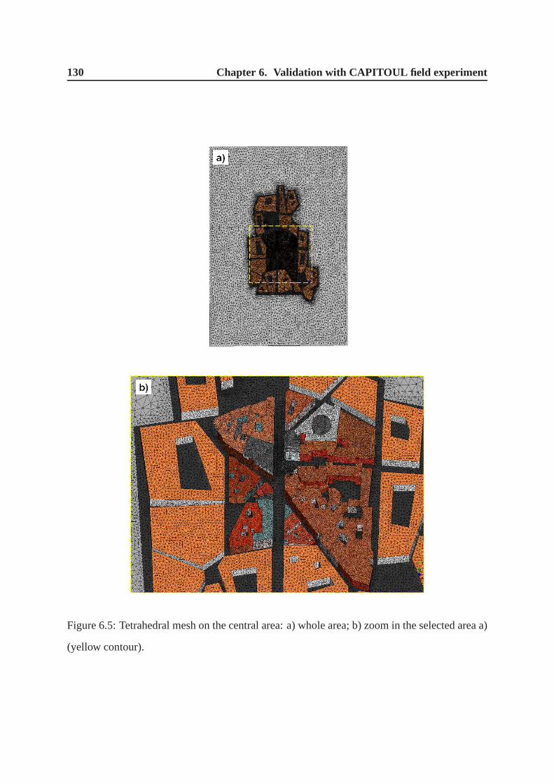
130 Chapter 6. Validation with CAPITOUL field experiment
Figure 6.5: Tetrahedral mesh on the central area: a) whole area; b) zoom in the selected area a)
(yellow contour).

6.4. Results and discussion 131
model, the ground temperature with force-restore method and the building surfaces (wall/roof)
temperature with a wall thermal model. The variation of the deep soil temperature is neglected.
Since most buildings in the center of Toulouse are from 19th century, walls are built with bricks
and most are not insulated as well as the roofs (Pigeon et al., 2008). Thus, at this stage, the
internal building temperature is calculated with a temperature evolution equation as equation
2.34. From some Toulouse pictures, we estimate the roughness value depending on its location
(e.g. 0.1m for roofs and walls in the center, 0.02m for street in the center and 1.5m for the
outside region) and set value for both dynamic roughness length and thermal roughness length.
Based onPigeon et al.(2008), we set the thermal properties such as surface conductivity and
thickness. We summarize the model parameters in Table6.1. Since the values fromPigeon et al.
(2008) are averages over the 500-m radius around the surface energy balance station, watching
some Toulouse pictures from Google Maps, we furthermore classify four wall painting color
(rose, gray, whitewash and white) for the buildings in the center area (Fig.6.4) to estimate the
albedo. Their values are given in Table6.2.
Modeling the urban energy balance in CAPITOUL consists in several steps. First we test
only the radiative scheme without introducing the convective exchange. Second we specify a
constant heat transfer coefficient to take into account a global wind field effects. Finally, we
model detailed variable wind fields and the effects of the full radiative-convective coupling on
the thermal transfer. For the full coupling study, since there is no wind field data available in
the street, we retains a degree of simplicity by modeling thewind profile under canopy height
with the exponential law ofMacdonald(2000) (see Chapter 3, Eq. 5a.14).
6.4 Results and discussion
6.4.1 Comparison of IRT pictures
A Thermal InfraRed (IRT) picture from for the aircraft flight432 of July 15, 2004 at 1412 UT
is shown in Figure6.7a. In Figure6.7b and6.7c, we depict respectively the modeled bright-

132 Chapter 6. Validation with CAPITOUL field experiment
0 2 4 6 8 10 12 14 16 18 20 22 24UT Hours
0
1
2
3
4
5
6
Win
d sp
eed
(m s
-1)
a)
0 2 4 6 8 10 12 14 16 18 20 22 24UT Hours
0
100
200
300
400
Win
d di
rect
ion
(°)
b)
0 2 4 6 8 10 12 14 16 18 20 22 24UT Hours
10
15
20
25
30
Air
tem
pera
ture
(°C
)
c)
Figure 6.6: Meteorological data at 47.5 m above the road from the CAPITOUL experiment
for 15 July 2004: a) Wind speed (m s−1), b) Meteorological wind direction (), and c) Air
temperature (C).

6.4. Results and discussion 133
Table 6.1: Parameters applied in the CAPITOUL simulations,symboles with same signification
as MUST simulation, see Chapter 3, Table 1.
Parameter Unit Value
Dynamic
Time-step s 10
Zre f m 47.5
Ure f ms−1 3.21
θ 340
Roofz0 cm 10
Wall z0 cm 10
Streetz0 cm 20
Radiative
Time-step min 15
Roofz0T cm 10
Wall z0T cm 10
Streetz0T cm 20
αS 0.08
εR 0.9
εW 0.92
εS 0.95
λR W K−1 m−1 0.83
λW W K−1 m−1 1.15
eR m 0.09
eW m 0.3
µS Jm−2s−0.5K−1 1330
Initial temperature values
TairC 18.86
Alsace East C 22.36/22.94
Alsace Road C 23.18/25
Alsace West C 21.32/22.23
Pomme SSWest C 24.70/25.55
Pomme Route C 23.33/25
Pomme NNEast C 29.06/29.78
Pomme Roof C 11.13/10.36

134 Chapter 6. Validation with CAPITOUL field experiment
Table 6.2: Albedo classfication of the buildings surfaces
Paint color albedo
White 0.6
Whitewash 0.5
Rose 0.3
Gray 0.15
ness temperature and surface temperature with the radiative-dynamic coupled model. Since we
distinguish different albedo from painting colors, the model reproduced well the heterogeneity
of the distribution of the brightness temperature, especially at roof level (Fig. 6.7b). We can
also note that if we were to keep more details especially someslopes on central roof in our
3D model to create a more detail distribution of the shadows on the roof, the simulated bright-
ness roof temperature would be closer to the observations. The value of the modeled surface
temperatures (Fig.6.7c) is obviously larger than the modeled brightness one (e.g.about 3C
difference on the roof), because from equation2.35, we can see that the brightness tempera-
ture is proportional to the product of the surface temperature and emissivity (the emissivity is
smaller than 1).
Figure6.8 from (a) to (d) shows the measured and modeled brightness temperatures for
the aircraft flight 431 at 1138 UT, compared with three modeling approaches: radiative model
only (Fig. 6.8b), radiative and a constant heat transfer coefficient (Fig.6.8c), and radiative-
dynamic full coupling (Fig.6.8d) using the hybrid thermal scheme for the streets and walls.
The constant heat transfer coefficient (Fig.6.8c) is set similar toHénon(2008); Hénon et al.
(2011b). The result of the first simulation (Fig.6.8b, radiative scheme alone) shows that the
brightness temperatures are obviously higher than measurements. For a visibility reason, an
additional black contour is drawn to show the building structures. Especially on the roof, the
difference is more than 25C. The modeledTbr is out of color range.

6.4. Results and discussion 135
Figure 6.7: Comparison between the Thermal infrared (TIR) airborne images, simulated bright-
ness temperatures and surface temperatures of July 15, 2004, at 1412 UT during flight 432
(Lagouarde et al., 2010): a) TIR picture (189× 118 pixels), source fromHénon(2008); b)
Modeled brightness temperature with full radiative-dynamic coupling; c) same as b) but for
modeled surface temperature.

136 Chapter 6. Validation with CAPITOUL field experiment
Either taking a constant heat transfer coefficient, i.e. assuming a constant wind field in the
domain or taking a variable heat transfer coefficient with full coupling i.e. more realistically
modeling the wind field, as expected, the results (Fig.6.8c and6.8d) show a much better
agreement with observation (Fig.6.8a) in comparison to radiative model only case (Fig.6.8b).
From this IRT picture with this view (Fig.6.8a), in spite of the fact that we did not keep
all the elementary details on the roofs with different orientations and slopes, the simulated
temperatures represent well the spatial variability of thetemperatures.
For the variablehf case, the model-observation difference rarely exceeds 10C (Fig. 6.8d).
We notice also in the measurement (Fig.6.8a) that for the same roof and same orientation, the
temperature may differ by more than 5C, for instance at the bottom right of the image. This
may be due to heterogeneities in materials and geometry which can not be all accounted for
by modeling each individual area (or even every detail). Forbuilding walls, either shaded or
sunlit, the difference between measurement (Fig6.8a) and simulation (Fig.6.8d) is generally
less than 5C. In the measurement, some horizontal faces (e.g. buildings at left in center) are
relatively warmer than others. This may be due to some external structures (e.g. balcony) that
are not modeled but were exposed to the sun and therefore received more solar heating (Hénon,
2008). Regarding the streets, a minimum of 3 cells were set for thewidth; the model is able to
simulate the sharpness of the shadow (Fig.6.8c and6.8d). The portion of the street brightness
temperatures near the buildings is well reproduced. The averaged difference is less than 3C
(Fig. 6.8d). The simulated sunny portion is underestimated by about 5C (Fig. 6.8d).
The difference between constanthf (Fig. 6.8c) case and variablehf case (Fig.6.8d) is
also evident. With the chosen value, the constanthf case shows an overcooling about 15C at
roof level, 4 to 5C at walls, 4C in shaded streets and 7C in sunlit streets (Fig.6.8c). The
difference is due to the overestimation of constant chosen value forhf at this moment. Actually,
the contribution of the variablehf may be more important on the surface and air temperature
when modeling the temporal evolution. For this reason, we perform the simulation with full
coupling for a diurnal evolution in the next section.
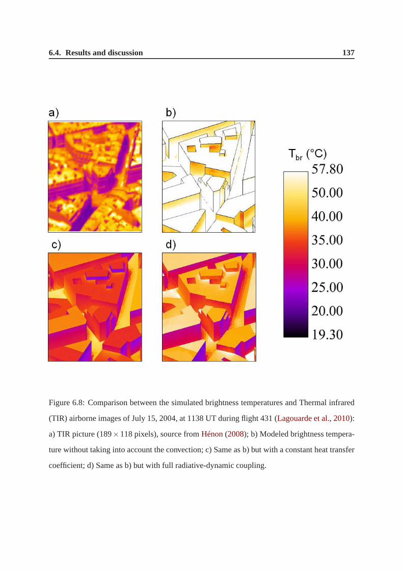
6.4. Results and discussion 137
Figure 6.8: Comparison between the simulated brightness temperatures and Thermal infrared
(TIR) airborne images of July 15, 2004, at 1138 UT during flight 431 (Lagouarde et al., 2010):
a) TIR picture (189×118 pixels), source fromHénon(2008); b) Modeled brightness tempera-
ture without taking into account the convection; c) Same as b) but with a constant heat transfer
coefficient; d) Same as b) but with full radiative-dynamic coupling.

138 Chapter 6. Validation with CAPITOUL field experiment
6.4.2 Comparison of the local diurnal evolution of brightness surface
temperature Tbr
Figure6.9a to c present the model-observation comparison for the brightness surface temper-
atures of the diurnal cycle of July 15 2004. The simulation isperformed with full radiative-
dynamic coupling. Hereafter, unless specified otherwise, all the results refer to full coupling
simulations. The infrared radiometers provided the measured brightness temperatures. Their
fixed positions around the central building of the study district are shown in Figure.6.10.
Overall, the diurnal evolutions of the brightness surface temperatures at the local positions in
the scene are correctly simulated.
For the faces of the Alsace street (black and red lines in Fig.6.9a), an overcooling about 5C
appears during the evening (1800 to 2400 UT). Since a similarremark has been found in MUST
case (see Chapter 3), it seems that the wall thermal model exhibits an underestimation on the
surface temperature after sunset. However, for the Alsace west face, the model predicts a higher
brightness temperature (red line in Fig.6.9a) from 0600 to 1200 UT. By using SOLENE model,
Hénon et al.(2011b) also report a similar difference in surface temperature. They explain that
this may be due to a sensor underestimation. The ground temperature is computed by the force-
restore method which is well adapted for the soil model. The bias on the Alsace road (green
line in Fig. 6.9a) can be explained by the approximation of the modeled shadow. Indeed, values
taken from the selected cell might be quite different from its neighborhood values.
The brightness temperature of the Pomme road is best predicted (magenta line in Fig.6.9b).
The primary model-observation disagreement occurs on Pomme northeast face (cyan line in
Fig. 6.9b) during the afternoon. The bias reaches 8C. We can call upon the same explanation
as for the Alsace road. Moreover, from some photos, we find that there are numerous windows
with white blind on this side of the wall. The infrared radiometer might detect a position
where white blinds were closed therefore more solar radiation flux was reflected. Or windows
were opened, the ventilation in the canopy led to a lower internal building temperature which
decreased the external temperature.

6.4. Results and discussion 139
The modeled roof brightness temperature displays a good agreement with observation be-
fore sunrise and from late afternoon to midnight (Fig.6.9c). However, the model exhibits
significant advance in warming when the roof start being sunlit. Actually, the sensor detecting
roof brightness temperature was fixed at a northern building’s roof from the mast (Fig.6.1a).
This building is treated as a simple block in the 3D model (Fig. 6.4). However, from figure
6.10.c, we can observe the complex structure of the roof. In particular, there are some small
obstacles which are higher than the measured roof to the eastbut are not represented in the
simulated scene. During the sunrise, the roof might be shaded due to these non modeled de-
tail structures. From the late afternoon, the sun shifts to another side. Since no more small
obstacles are higher than the measured roof, the bias disappears.
6.4.3 Model-Observation comparison of heat fluxes
I recall here one advantage of our model is that the determination of the heat fluxes is not only
at solid faces but also in the whole fluid domain. In order to comparer the fluxes data, we set
two monitoring points in the computational domain. One is atthe same location as the actual
sensors on the top of the mast (47.5m) (Fig. 6.4). Another is set on the roof surface where the
mast is placed (20m).
6.4.3.a Sensible heat fluxQH
The sensible heat flux at the surface can be recorded easily inthe simulation (cf. Eq.1.7) and
be compared to the value measured on the mast computed using eddy-covariance technique.
Here, we assume that the vertical sensible flux is conserved between the surface and its value
at sensor level. The horizontal advection of heat is therefore assumed negligible.
Figure6.11depicts the comparison between the time evolution of calculated sensible flux
at roof surface and the mast observation. Reasonable agreement generally exists between cal-
culated and measured values. Difference between observed and calculated values are less than
40Wm−2, except for the night (45−70Wm−2). From midnight to 0700 UT, the wind is calm
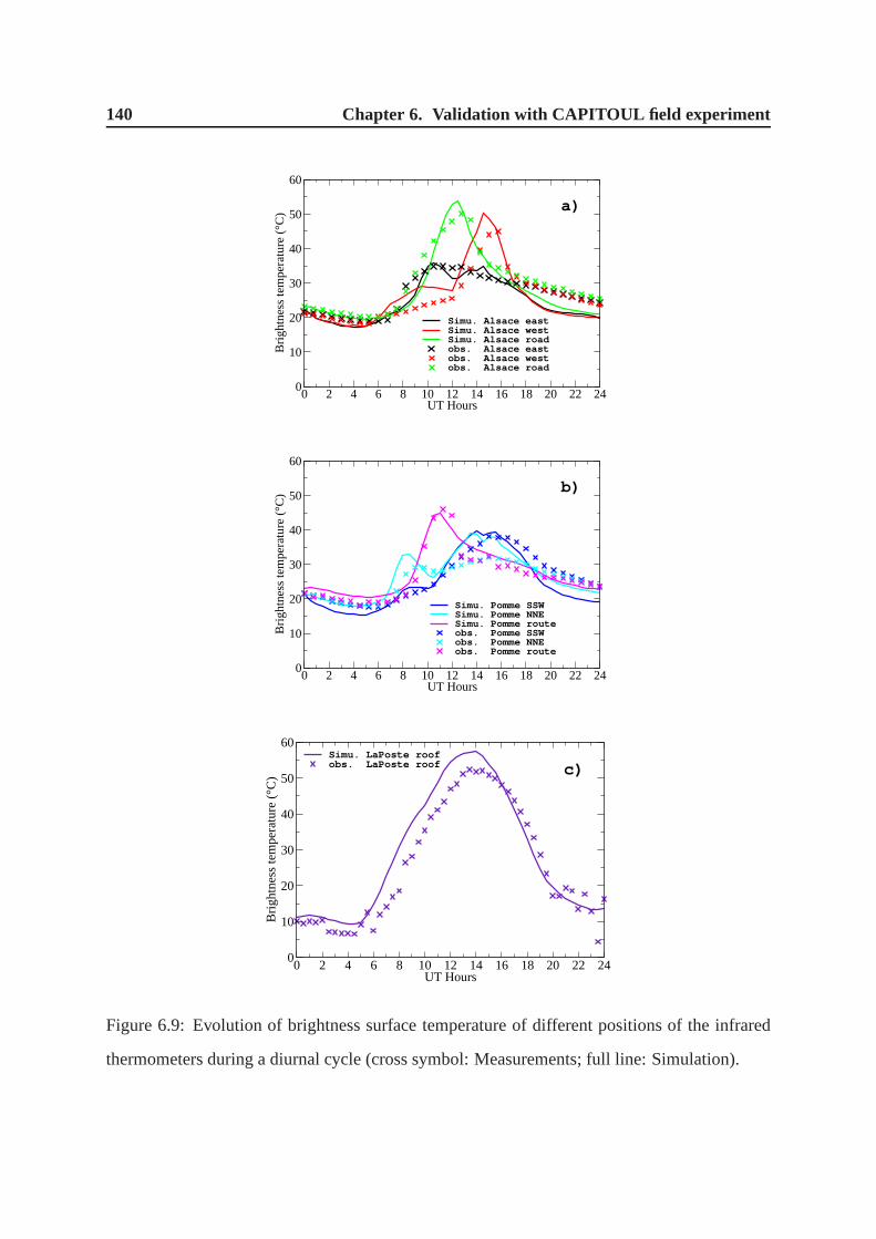
140 Chapter 6. Validation with CAPITOUL field experiment
0 2 4 6 8 10 12 14 16 18 20 22 24UT Hours
0
10
20
30
40
50
60
Brig
htne
ss te
mpe
ratu
re (
°C)
Simu. Alsace eastSimu. Alsace westSimu. Alsace roadobs. Alsace eastobs. Alsace westobs. Alsace road
a)
0 2 4 6 8 10 12 14 16 18 20 22 24UT Hours
0
10
20
30
40
50
60
Brig
htne
ss te
mpe
ratu
re (
°C)
Simu. Pomme SSWSimu. Pomme NNESimu. Pomme routeobs. Pomme SSWobs. Pomme NNEobs. Pomme route
b)
0 2 4 6 8 10 12 14 16 18 20 22 24UT Hours
0
10
20
30
40
50
60
Brig
htne
ss te
mpe
ratu
re (
°C)
Simu. LaPoste roofobs. LaPoste roof c)
Figure 6.9: Evolution of brightness surface temperature ofdifferent positions of the infrared
thermometers during a diurnal cycle (cross symbol: Measurements; full line: Simulation).

6.4. Results and discussion 141
Figure 6.10: From a) to c), different positions of the infrared thermometers. Source Pigeon
(2004).

142 Chapter 6. Validation with CAPITOUL field experiment
0 2 4 6 8 10 12 14 16 18 20 22 24UT Hours
0
100
200
300
400
500
Sen
sibl
e he
at fl
ux (
W/m
²)Simu. at roof surfaceobs. on mast
Figure 6.11: Diurnal variation of sensible heat flux calculated at roof surface (full line) and
measured on the mast (cross symbol).
but does not have a zero speed (Fig.6.6a) and the air temperature varies from 15 to 19C (Fig.
6.6c). The observed sensible flux is very small (cross symbol in Fig. 6.11), this maybe due to
the fact that the air layer just above the roof has a temperature very close the roof temperature.
However, the initialized roof temperature at this positionis set to the same value as the mea-
sured roof temperature (11.13C in Table6.1). With a non zero heat transfer coefficient and
a higher air temperature, consequently, negative sensibleheat flux is obtained at roof surface
(full line in Fig. 6.11). For the rest of the day the comparison is rather good.
6.4.3.b Outgoing long-wave radiative fluxL↑
Figure6.12shows the model-observation comparison of long-wave radiation flux. The differ-
ence between the modeled outgoing long-wave radiation flux at roof surface (full line) and on
the mast (dashed line) is generally less than 20Wm−2. However, both of them give an underesti-
mation of about 20Wm−2 during the night and a maximum overestimation of about 100Wm−2
in daytime. In fact, these differences are related to the error of on the roof temperature, i.e.
underestimation in the night and overestimation in the day.From equation1.6, we can see the

6.4. Results and discussion 143
outgoing infrared radiation flux highly depends on the surface temperature because of the term
of εσT4s f c.
0 2 4 6 8 10 12 14 16 18 20 22 24UT Hours
300
400
500
600
700
Rad
iatio
n flu
x (W
/m²)
Simu. at roof surfaceSimu. on mastobs. on mast
Figure 6.12: Diurnal variation of outgoing infrared flux calculated at roof surface (full line), at
the mast level (dashed line) and measured on the mast (cross symbol).
To complete the discussion, we have the advantage with the model to be able to visualize the
radiative flux in the computational domain. Fig.6.13illustrates the distribution of the outgoing
infrared flux at 1030 UT on the vertical center-plane and on the building surfaces. Significant
variability can be observed on the center-plane. Relatively high values are found at horizontal
solid-air interface due to the fact that horizontal surfaces are warmer than the vertical surfaces
in the daytime.
6.4.3.c Outgoing global radiative fluxS↑
Figure6.14compares the modeled upward global solar flux with the measured one. The non-
zero measured nighttime solar flux may be due to the sensor errors or the artificial lights from
shop-windows, cars and street-lamps (Hénon et al., 2011b). The upward solar flux can be
estimated by equation1.5. For this gray roof (Fig.6.9.b), we set an albedo of 0.15 (Table6.2).

144 Chapter 6. Validation with CAPITOUL field experiment
Figure 6.13: Visualization of the outgoing infrared flux on the center-plane and surfaces at
1030 UT. The north, wind and sun direction are indicated.
The same value is also proposed byPigeon et al.(2008) and is used inHénon et al.(2011b).
Compared to the observation, in spite of about 20Wm−2 higher values at noon estimated by the
model (full line), the agreement between measurement and modeled the outgoing solar flux on
mast (dashed line) is very satisfactory.
In the same manner as for the long-wave radiative flux, in Figure 6.15we display the dis-
tribution of the outgoing global solar flux at 1030 UT on the center-plane and on the surfaces.
Through the visualization the propagation of the radiativeflux in the fluid domain, we can bet-
ter understand the distribution of the shadow projected by the different structures. We can also
readily identify surfaces with higher albedo since they reflect more solar radiation flux.
6.4.4 Model-Observation comparison of friction velocityu∗
Friction velocityu∗ (m s−1) is also measured on the mast during the CAPITOUL experiment.
Theu∗ at the roof surface is defined by the relation:
u∗ = (|τw/ρ|)1/2, (6.1)

6.4. Results and discussion 145
whereτ is the Reynolds stress at wall (N), ρ (kg m−3) the fluid density at the wall.
In order to compare with the observation on the mast, we use the kinematic momentum
0 2 4 6 8 10 12 14 16 18 20 22 24UT Hours
0
30
60
90
120
150
180
Rad
iatio
n flu
x (W
/m²)
Simu. at roof surfaceSimu. on mastobs. on mast
Figure 6.14: Same as Fig.6.12but for outgoing solar flux.
Figure 6.15: Same as Fig.6.12but for outgoing solar flux.

146 Chapter 6. Validation with CAPITOUL field experiment
fluxes in thex andy directions (u′w′, v′w′), therefore the friction velocity can be evaluated as:
u∗ = (u′w′2+v′w′2)1/4, (6.2)
whereu′w′ andv′w′ are given by:
u′w′ = νt∂u∂z
, v′w′ = νt∂v∂z
, (6.3)
andνt is the turbulent viscosity given by thek− ε closure.
From Figure6.16it can be seen that the simulated friction velocities are reasonable in terms
of magnitude. Modeled friction velocity at roof surface (full line) shows a good agreement with
observation when theu∗ less than 0.2m s−1. Simulatedu∗ on mast (dashed line) can produce
higher value (0.4m s−1). It seems that the model overestimates the nighttime (1800− 2400
UT) u∗ on mast. However, estimates ofu∗ from the turbulence measurements by the sonic are
known to be rather uncertain, especially whenu∗ is small. The difference between the modeled
u∗ at roof surface (full line) and at the mast level (dashed line) is due to different methods of
the estimation, and the numerical errors in the computed gradients.
0 2 4 6 8 10 12 14 16 18 20 22 24UT Hours
0
0,1
0,2
0,3
0,4
0,5
0,6
Fric
tion
velo
city
(m
/s)
Simu. at roof surfaceSimu. on mastobs. on mast
Figure 6.16: Same as Fig.6.12but for friction velocity.

6.4. Results and discussion 147
6.4.5 Statistical comparison with hand-held IRT data
Regarding hand-held IRT measurement, several groups of records for different surface types in
the study center are available in the database (e.g. Fig.6.7). In order to statistically analyze
simulation results with these data, we select the samples obtained in the Alsace street (Fig.
6.17a) at 0945 UT, 1245 UT and 1545 UT for the day of 15th July 2004 and calculate the
averaged values, standard deviation and median values for the predicted brightness temperature
in a similar zone from the computational domain as shown in Figure6.17b. The results are
tabulated in Tables6.3, 6.4and6.5.
Note that the number of observations that are available to conduct the statistical analysis
is often very small. Only records for building walls and street (excluding the roof elements)
are available for this database. The data of the street consists of two parts, road and sidewalk.
However, we have only a flat ground in our 3D model. For that reason, from our simulation
result, we consider that the cells next to the buildings footbelong to the sidewalk part and the
central part of the street is the road. Moreover, values in the database were separated into sunlit
and shaded part. In order to give a criteria to separate facets in the simulation, we look at the
direct solar flux value received by the surfaces. That is, fora given facet, if the direct flux is less
than 50Wm−2 (we discuss the sensitivity to that value later in the text),we consider that it is in
the shadow. Otherwise, it is sunny. In addition, if a value isnot available in the measurement
or does not meet the criteria in the simulation, we set ‘N/A’ in the tables.
From Table6.3, we observe that all the westward walls are shaded at 0945 UT.The model
gives higher average and median values (about 4 to 7C). The results from the facets exposed
under the sun conform better with expectation, especially for the sidewalk and eastward walls.
The difference between prediction and observation is about2 to 4C for the mean temperature.
The pavement prediction shows a better agreement with observation for mean and median
temperature but with a relatively important standard deviation (6.2 in Tab.6.3).
The overall result conveyed by Table6.4 is disappointing. Most of westward walls from
the model are judged to be sunlit. Significantly higher values are found fir road and pavement

148 Chapter 6. Validation with CAPITOUL field experiment
Figure 6.17: Selected zone for statistical study: a) Alsacestreet view, from Google maps; b)
selected urban blocks in 3D model (in color).

6.4. Results and discussion 149
0945 UT Sunlit Shaded
Simulated Measured Simulated Measured
W
Average N/A N/A 27.3 20.8
St. Dev. N/A N/A 1.3 0.7
Median N/A N/A 27.5 20.8
Max N/A N/A 29.6 21.7
Min N/A N/A 23.7 19.9
Road
Average 33.5 27.2 27.0 20.6
St. Dev. 5.7 N/A 0.8 0.2
Median 32.2 N/A 27.1 20.7
Pd
Average 32.6 30.0 26.9 20.1
St. Dev. 6.2 3.4 0.8 0.7
Median 30.0 30.0 27.0 20.1
E
Average 37.5 33.2 25.1 20.4
St. Dev. 3.5 4.8 1.7 1.1
Median 36.9 33.8 24.4 20.0
Max 47.3 38.6 27.9 22.2
Min 28.4 26.3 22.5 19.2
Table 6.3: Statistical comparison of modeled brightness temperature (C) and hand-held IRT
data (C) at 0945 UT with:Sunlit, Shadedvalues from sunny and shaded conditions, respec-
tively; Simulated, Measuredmodeled and observed values, respectively;St. Dev. stand devi-
ation; N/A no available value;W, E wall facing west and east respectively;Roadmiddle of
street;Pd sidewalk.

150 Chapter 6. Validation with CAPITOUL field experiment
1245 UT Sunlit Shaded
Simulated Measured Simulated Measured
W
Average 34.2 N/A 28.7 24.4
St. Dev. 2.4 N/A 0.0 0.7
Median 34.3 N/A 28.7 24.3
Max 54.1 N/A 28.7 25.8
Min 28.1 N/A 28.7 23.7
Road
Average 52.9 37.2 51.8 23.0
St. Dev. 1.7 7.9 2.7 0.3
Median 52.6 34.2 52.0 23.0
Pd
Average 50.9 40.0 49.2 22.6
St. Dev. 5.1 0.6 1.4 0.2
Median 50.9 40.0 50.3 22.7
E
Average 43.7 34.4 32.2 26.4
St. Dev. 5.0 1.6 3.1 2.3
Median 45.8 35.0 32.1 26.4
Max 49.9 36.4 40.3 28.1
Min 35.7 30.9 27.7 24.8
Table 6.4: Same as Tab.6.3but for 1245 UT.

6.4. Results and discussion 151
1545 UT Sunlit Shaded
Simulated Measured Simulated Measured
W
Average 40.8 32.8 29.9 N/A
St. Dev. 6.2 2.5 0.8 N/A
Median 40.8 32.5 29.9 N/A
Max 55.1 37.3 33.5 N/A
Min 29.2 28.8 28.1 N/A
Road
Average N/A 45.8 35.9 36.2
St. Dev. N/A 4.8 1.7 1.6
Median N/A 48.0 35.6 36.2
Pd
Average 50.5 46.4 35.9 22.6
St. Dev. 3.5 0.7 3.3 5.9
Median 50.4 46.4 34.4 33.5
E
Average 41.8 N/A 31.3 30.2
St. Dev. 3.8 N/A 2.1 0.9
Median 40.0 N/A 30.8 30.2
Max 47.4 N/A 37.7 31.5
Min 37.5 N/A 28.1 28.9
Table 6.5: Same as Tab.6.3but for 1545 UT.

152 Chapter 6. Validation with CAPITOUL field experiment
(more than 10C) than measurements. It seems that the model fails to predict the low tem-
perature of either the shaded road or sidewalk. We notice that either for road or sidewalk, the
predicted average and median temperature in shadow is very close to the sunlit one. However,
as mentioned above, the threshold set is only 50Wm−2 from predicted direct solar flux value. It
means that the high temperatures from shaded road and sidewalk are not due to heating by the
direct solar radiation but probably due to received diffusesolar or infrared radiation and also
the multi-reflected radiation by surrounding buildings. Since we can see many shop windows in
this commercial street in Figure6.17a, the model may overestimate the multi-reflection without
modeling the glass (Fig.6.17b). Moreover, the presence of smaller obstacles (e.g. vehicles,
traffic signs, fences, etc.) increase the percent cover of shaded surface. A large standard devi-
ation in the observation for the sunlit road (7.9 from Tab.6.4) shows that the street may have
heterogeneities on the surface (e.g. albedo) and materials(e.g. asphalt, concrete, stone). The
model gives such result without including these details.
The corresponding results for 1545 UT (Tab.6.5) are better than for 1245 UT. The shaded
elements have the best performance. Bias of the predicted average and median temperatures
are only about 1C. The modeled sunlit elements have less accuracy. The overestimations of
average and median temperature on the westward walls (about8C) are due to some extremely
high predicted values. No available values appear for the predicted sunlit road part but not for
the pavement. We can explain that the chosen resolution of the road may be insufficient. It
leads to the fact that the cells over the threshold appear as pavement.
For this statistical assessment, we have also tested 100Wm−2 as threshold criteria, but the
model result seems not very sensible to this criteria. For instance, averaged temperatures of the
sunlit and shaded westward wall at 1545 UT are 41.7 and 30.2C respectively against 40.8 and
32.8C as found in Table6.5.

6.5. Conclusions and perspectives 153
6.5 Conclusions and perspectives
We have investigated the energy exchanges in a real city withthe atmosphere during the
CAPITOUL campaign, using new atmospheric radiative and thermal schemes implemented in
Code_Saturne. A pre-processing is realized including the optimization of the complex geom-
etry and creation of a high quality tetrahedral mesh for thisstudy. It also requires determining
the complex thermal parameters which take into account the actual variability of materials in
the district. Based on the literature data, we have separated the building surface into 4 classes
of albedo depending on painting colors.
First, simulations are evaluated with the comparison with Thermal InfraRed airborne im-
ages from two flights in the day of 15th July 2004 during the CAPITOUL project. The result
shows the importance of taking into account heterogeneities in materials and geometry to repre-
sent the spatial variability of the temperatures in complexurban areas. Then, we have evaluated
the coupled dynamic-radiative model with CAPITOUL experiment including the comparison
with the measured brightness temperature, sensible flux, radiative fluxes diurnal variation, and
statistical values with hand-held IRT data. Overall the agreement between measurements and
model simulations are fair but can be improved in the future with more information. For the
sensible flux, the model-observation nighttime bias is probably linked to the uncertainty of the
estimation on the roof nighttime temperature. Similar explanation can be used for the com-
parison of the outgoing infrared flux, because results are sensitive to the surface temperature.
Better agreement is obtained for the comparison of the outgoing solar flux at the mast level.
However, the difference between the modeled outgoing solarflux at roof surface and at the mast
is still unclear. For the modeled friction velocities, the difficulty mainly appears to capture the
extreme values (highest or lowest). Small structures may have important influence on the com-
putation of local brightness surface temperature, sensible flux, outgoing short- and long-wave
radiation. The simulation results shows the importance of modeling in details while doing local
model-observation comparison. The statistical analysis,while comprehensive, is not exhaus-
tive. Despite the fact that difference between measured andmodeled averaged, median and

154 Chapter 6. Validation with CAPITOUL field experiment
standard deviation of brightness surface temperature may be significant, such comparison is
very useful for a better understanding of the radiative transfer processes in the canopy.
The model results are encouraging and give insight into local surface-atmosphere processes,
but further and more rigorous testing has to be performed, especially regarding vertical sensible
flux and upward infrared flux.

CHAPTER 7
Conclusions and Future Work
Contents
7.1 Summary and Conclusions . . . . . . . . . . . . . . . . . . . . . . . . . . . . 155
7.2 Perspectives . . . . . . . . . . . . . . . . . . . . . . . . . . . . . . . . . . . . 158
7.1 Summary and Conclusions
A three-dimensional numerical atmospheric radiative transfer scheme coupled with a CFD code
to simulate the urban surface energy balance (SEB) has been developed. Validations of the full
radiative-convective coupling are performed through a comparison with observation datasets
from MUST (idealized built-up area, Chapter 3) and CAPITOUL(real urban environment,
Chapter 6) field experiments.
The improvement of the heat transfer model in buildings and the study of the full radiative-
convective coupling, are addressed in Chapters 3 and 6. The model successfully simulates a
key parameter in the SEB, the surface temperature, for different sides of a container within the
MUST canopy in a diurnal cycle (see Chapter 3) and also a 24 hours evolution of the brightness
surface temperature for different positions in the district within the CAPITOUL study center
area (see Chapter 6). The model incorporates two approachesto model heat transfer with
buildings: the force-restore scheme and the wall thermal model. Tests of the performance of
these two approaches show that to explicitly treat the heat conduction, even with only one-layer,
the wall thermal model is more adapted for the building wallsthan the force-restore approach

156 Chapter 7. Conclusions and Future Work
which was originally developped for the soil model (see Chapter 3). By taking advantage of the
force-restore approach and the wall thermal model to separately model the ground and building
walls temperatures, a hybrid surface temperature scheme shows a good ability when applied to
the CAPITOUL case (see Chapter 6). In case of buildings without good insulation, the internal
building temperature has a large influence on the surface temperature in the diurnal cycle (see
Chapter 3). As a solution, an evolution equation obtained from the literature is adopted to
more realistically model the internal building temperature. In any case the improvement of the
surface model has been identified as an area for future work.
Results from Chapter 3 and 6 also illustrate quantitativelyhow the sensible heat flux plays
an important role in SEB. For instance, in MUST case (see Chapter 3), a difference of about 10
to 30C on the surface temperature is obtained when including or not the convection. Moreover,
in Chapter 3, we have discussed and compared different approaches to estimate the sensible
flux: constant heat transfer coefficient, using a 1D equationbased on a vertical wind profile
within the canopy and our 3D modeling approach. This comparison shows a difference about
4C on the wall. Thus we conclude that a good description of the heat transfer coefficient and
its spatial variability is essential to determine the sensible heat flux in the canopy.
Based on MUST full radiative-convective validation, the atmospheric radiation model in
Code_Saturne is well-tested in Chapter 4 to achieve the objective of comparison with the ge-
ometric view factor approach, used by the SOLENE model. The most significant differences
between the two models are for the diffuse solar flux, due partly to an assumption of the homo-
geneous incoming diffuse solar flux from simple clear sky model in Code_Saturne. Neverthe-
less, results show that the two models agree well with each other for the time evolution of the
direct solar flux, incident infrared flux and surface temperature, because the diffuse solar fluxes
are small.
Chapter 5 serves primarily as a demonstration of the abilityof our radiative model to in-
vestigate the thermal effect of buildings on the local atmospheric flow under low wind speed
condition. In this short-term study, the results show that taking into account the thermal strat-

7.1. Summary and Conclusions 157
ification has a significant influence on the wind field. The difference between the case for
which we impose the temperatures and the case with temperatures calculated with 3D radiative
transfer case can also be important. Moreover, under radiative condition, the temperature and
vertical motion show a great sensitivity to change in the physical parameters of the wall sur-
faces. We illustrate that increasing the albedo from 0.1 to 0.6 (e.g. painting a dark surface to
white) reduces the net radiation flux term in the surface energy balance (SEB), as a result, the
temperature close to the windward wall or roof may decrease by 2C.
The results from the CAPITOUL case described in Chapter 6 have addressed the last ob-
jective: the validation of our approach on a real city district. The generation of the CAPITOUL
complex mesh requires a important preliminary work to optimize the geometry, and in addi-
tion, we have separated 4 classes of albedo value depending on wall painting colors. Through
the comparison with the Thermal InfraRed airborne images from two flights in the day of 15th
July 2004, we demonstrate the importance of taking into account heterogeneities in materials
and geometry to reproduce the spatial variability of the temperatures in complex urban areas.
Moreover, the full coupling is tested against in situ observation during the same day. The re-
sults show that to perform well overall in terms of the brightness temperature (with hybrid
temperature scheme). The model predicts a good daytime sensible flux, but shows a night-
time underestimation. Similar comments can be made for the model-observation comparison
of the outgoing infrared flux. Regarding the outgoing solar flux, the result shows an excellent
model-observation agreement at the mast position. In the statistical study, some significant
differences between the predicted and observed mean, median, standard deviation brightness
temperature are identified. Despite of some significant differences between the predicted and
observed statistics of brightness temperatures, the analysis provides an interesting and different
approach to evaluate the model performance.

158 Chapter 7. Conclusions and Future Work
7.2 Perspectives
There are still a number of directions avenues which remain to be investigated or which have
opened during this work.
The application of our radiative-dynamical coupled model for the CAPITOUL case could
be extended through more model-observation comparisons, in particular for a winter day. Fur-
ther improvements should be considered, such as the buildings in the region outside which are
treated at present with a high roughness value, but should betreated with a drag-porosity ap-
proach which will permit a more realistic modeling of the wind profile in the canopy. If the
anthropogenic heat flux is not significant in a summer day, it may not be neglected in winter.
Thus the model should properly include variation of diurnalanthropogenic flux, eventually by
using a formula proposed byPigeon et al.(2008). The one-layer wall thermal model we used
show some limitations. In MUST case, it can reproduce the diurnal cycle of the different sur-
face temperature only with a very low thermal conductivity.Either in MUST or in CAPITOUL,
a nighttime overcooling appears by using this scheme. We expect that the implementation of
a multilayer wall thermal model may lead to improvements andcan improve the temperature
overestimation during the day.
The comparison ofCode_Saturne and SOLENE radiation models and the numerical study
of a low wind speed case in Chapter 4 and 5 respectively may be supplemented with more real
measurement data set. Furthermore, in comparing the two radiation models, taking diffuse so-
lar flux values from SOLENE as boundary conditions shows an improvement inCode_Saturne.
Full implementation of a similar sky model as in SOLENE with non-uniform diffuse solar ra-
diation distribution may be necessary inCode_Saturne when applications are under cloudy
weather condition. The comparison also can be extended to other field experiments, such as
with results presented byHénon et al.(2011b) from CAPITOUL datasets, or to compare with
other radiation models, e.g. SYRTHES (SYstèm de RésolutionTHErmique Solide) (Péniguel
and Rupp, 2008). SYRTHES is a thermal code for a larger number industrial applications
and has become open-source also. The thermal solver can be used alone if only by conduc-

7.2. Perspectives 159
tion/radiation problems or coupled withCode_Saturne or other fluid mechanics codes.
In the model presented in this work, the atmosphere at the microscale is considered to be
transparent and non-diffusive. One of the perspective of this work is to use the 3D radiative
scheme for nontransparent media, for applications like assessment of pollutant dispersion or
fog formation and dissipation etc. Absorption and diffusion have significant importance. Ab-
sorption can already be taken into account by our scheme, so it requires adding the diffusion
term in the resolution of the radiative transfer equation.
Regarding the dynamical aspect, in the present work, the turbulence is parameterized by
the Reynolds-averaged Navier-Stokes (RANS) (more specifically, the standardk− ε closure)
approaches due to the limitations on computational cost. Itis well known that conventionalk−
ε models, with the turbulent viscosity formulation, tend to overestimate the level of turbulent
kinetic energy around the stagnation point. In order to increase the accuracy of the prediction of
the airflow around buildings, one direction of future work isto use the Large Eddy Simulation
(LES) approach for the convective model. If the computational cost remains too high for the
whole day simulation, at least, LES can be applied for the shorten study such as the low wind
speed case described in Chapter 5.
Finally, tests of the full model are limited to two days at twoseparate sites, and should be
performed for a greater range of urban sites, weather conditions and seasons to more success-
fully separate model weaknesses from incorrect parameter specification and/or processes influ-
encing the observations. For instance, a more recent field experiment, Towards optimisation
of urban-planning and architectural parameters for energyuse minimisation in Mediterranean
cities (TOPEUM) campaign has been carried out in the city of Nicosia, in Cyprus in July 2010
(Neophytou et al., 2011). The main objective of TOPEUM is to investigate the influence of dif-
ferent urbanisation characteristics (such as the geometryand density of buildings within a city
and the type of building materials used) on the intensity of the urban heating effect in the case
of a typical Mediterranean city, such as a Cypriot urban area. The field measurements include
meteorological measurements as well as on-ground and aerial thermal infrared pictures, cover-

160 Chapter 7. Conclusions and Future Work
ing a range of spatial scales, from local-street canyon to meso-scale. The measurements record
the meteorology, the resulting local microclimate, particularly in the street and the thermal
response of the buildings in the field area, especially the building inside temperature measure-
ment. This can provide a good verification for the accuracy ofthe evolution equation which we
used to estimate the internal building temperature.

Bibliography
Antoine, M. J. and D. Groleau, 1998: Assessing solar energy and environmental variables in
urban outdoor spaces: Towards a simulation and monitoring tool. Rebuild the European
cities of Tomorrow : Shaping our European cities for, for the21st Century Proccedings of
the 2nd European Conference, Florence, Italy (April 1-3, 1998).73, 74
Archambeau, F., N. Méchitoua, and M. Sakiz, 2003: Code_Saturne : a Finite Volume Code for
the Computation of Turbulent Incompressible Flows - Industrial Applications.Int. J. Finite.
Volumes, 1, 1–62.39
Arnfield, A. J., 2003: Two decades of urban climate research:A review of turbulence, ex-
changes of energy and water, and the urban heat island.Int. J. Climatol., 23 (1), 1–26.50
Asawa, T., A. Hoyano, and K. Nakaohkubo, 2008: Thermal design tool for outdoor space based
on a numerical simulation system using 3D-CAD.Build. Environ., 43, 2112–2123.68
Baldwin, B. S. and H. Lomax, 1978: Thin layer approximation and algebraic model for sepa-
rated turbulent flows.AIAA, 78–257.18
Best, M. J., C. S. B. Grimmond, and M. G. Villani, 2006: Evaluation of the urban tile in
MOSES using surface energy balance observations.Bound.-Layer Meteor., 118, 503–525.
36
Bird, R. E. and R. L. Hulstrom, 1981: A simplified clear sky model for direct and diffuse
insolation on horizontal surfaces. Tech. Rep. SERI/TR-642-761, Solar Research Institute, 38
pp., Golden, Colorado.45, 46, 77
Blocken, B., 2009: Pedestrian wind comfort around a large football stadium in an urban en-
vironment: CFD simulation, validation and application of the new Dutch wind nuisance
standard.J. Wind Eng. Ind. Aerod., 97, 255–270.16

162 Bibliography
Blocken, B., T. Defraeye, D. Derome, and J. Carmeliet, 2009:High-resolution CFD simulations
for convective heat transfer coefficients at the facade of a low-rise building.Build. Environ.,
44, 2396–2412.16
Blocken, B., T. Stathopoulos, and J. Carmeliet, 2007: CFD simulation of the atmospheric
boundary layer: wall function problems.Atmospheric Environment, 41, 238–252.26
Boussinesq, J., 1877: Essai sur la theories des eaux courantes.Memoires presentes par divers
savants a lâAcademic des Sciences de lâInstitut National deFrance, 23, 46–50.18
Bouyer, J., 2009: Modélisation et simulation des microclimats urbains: Étude de lâimpact
de lâaménagement urbain sur les consommations énergétiques des bâtiments. Ph.D. thesis,
École Polytechnique de l’Université de Nantes, 306 pp., [inFrench].70
Briggen, P. M., B. Blocken, and H. L. Schellen, 2009: Wind-driven rain on the facade of
a monumental tower: numerical simulation, full-scale validation and sensitivity analysis.
Build. Environ., 44, 1675–1690.16
Camuffo, D. and A. Bernardi, 1982: An observational study ofheat fluxes and the relationship
with net radiation.Bound.-Layer Meteor., 23, 359–368.12
Casey, M. and T. Wintergerste, 2000: Best Practice Guidelines, ERCOFTAC Special Interest
Group on Quality and Trust in Industrial CFD. Tech. rep., Fluid Dynamics Laboratory Sulzer
Innotec, ERCOFTAC, Brussels.18, 20
Chapman, D. R., 1979: Computational aerodynamics development and outlook.AIAA, 17,
1293–1313.17
Chen, F., H. Kusaka, M. Tewari, J. Bao, and H. Hirakuchi, 2004: Utilizing the coupled
WRFLSMUrban modeling system with detailed urban classification to simulate the urban
heat island phenomena over the Greater Houston area.Fifth Conference on Urban Environ-
ment, Vancouver, BC, Canada, Amer. Meteor. Soc., CD-ROM. 9.11.36

Bibliography 163
Coceal, O., A. Dobre, T. G. Thomas, and S. E. Belcher, 2007: Structure of turbulent flow over
regular arrays of cubical roughness.Bound.-Layer Meteor., 589, 375–409.17
Cook, M., Y. Ji, and G. Hunt, 2003: CFD modelling of natural ventilation: combined wind and
buoyancy forces.Int. J. Ventilation, 1, 169–180.16
Courant, R., K. Friedrichs, and H. Lewy, 1967: On the partialdifference equations of mathe-
matical physics.IBM Journal, 215–234.20
Dandou, A., M. Tombrou, E. Akylas, N. Soulakellis, and E. Bossioli, 2005: Development and
evaluation of an urban parameterization scheme in the Penn StateNCAR Mesoscale model
(MM5). J. Geophys. Res., 110, D10 102.36
Davidson, P. A., 2004:Turbulence - An Introduction for Scientists and Engineers. Oxford
University Press, 678 pp.16
Deardorf, J. W., 1978: Efficient prediction of ground surface temperature and moisture with
inclusion of a layer of vegetation.J. Geophys. Res., 83, 1889–1903.47, 48
Douce, A. and N. Méchitoua, 2003: Mise en oeure dans des modélisations physiques par-
ticulière Tome 3: Transfert thermique radiatif en milieux gris semi-transparents. Rapport
interne edf, in French, EDF R&D, Fluid Mechanics and Heat Transfert Department.43
Dupont, S. and P. G. Mestayer, 2006: Parameterization of theurban energy budget with the
submesoscale soil model.J. Appl. Meteor. Climatol., 45, 1744–1765.36, 48
Dupont, S., T. L. Otte, and J. K. S. Ching, 2004: Simulation ofmeteo-rological fields within
and above urban and rural canopies with a mesoscale model (MM5).Bound-Layer. Meteorol.,
113, 111–158.33
Fiveland, W. A., 1984: Discrete-ordinates solutions of theradiative transport equation for rect-
angular enclosure.J. Heat Tran., 106, 699–706.45

164 Bibliography
Fortuniak, K., B. Offerle, and C. S. B. Grimmond, 2005: Application of a slab surface energy
balance model to determine surface parameters for urban areas.Lund eRep. Phys. Geog., 5,
90–91.36
Franke, J., A. Hellsten, H. Schlünzen, and B. Carissimo, 2007: Best Practice Guideline for the
CFD simulation of flows in the urban environment: COST Action732: Quality Assurance
and Improvement of Microscale Meteorological Models. Tech. Rep. ISBN 3-00-018312-4,
COST Office Brussels.18, 19, 20, 21, 22, 23, 24, 25, 27, 31, 32, 127
Gastellu-Etchegorry, J. P., 2008: 3D modeling of satellitespectral images, radiation budget and
energy budget of urban landscapes.Meteor. Atmos. Phys., 102, 187–207.34, 42, 68, 127
Gastellu-Etchegorry, J. P., E. Martin, and F. Gascon, 2004:Dart: A 3-d model for simulating
satellite images and surface radiation budget.Int. J. of Remote Sens., 25, 75–96.34, 127
Grimmond, C. S. B. and T. R. Oke, 1999a: Aerodynamic properties of urban areas derived
from analysis of surface form.J. Appl. Meteor., 38, 1262–1292.33
Grimmond, C. S. B. and T. R. Oke, 1999b: Heat storage in urban areas: Local-scale Observa-
tions and Evaluation of a Simple model.J. Appl. Meteor., 38, 922–940.12
Grimmond, C. S. B. and T. R. Oke, 2002: Turbulent heat fluxes inurban areas: Observations &
local-scale urban meteoro-logical parameterization scheme (LUMPS).J. Appl. Meteor., 41,
792–810.32
Grimmond, C. S. B., et al., 2010: The International Urban Energy Balance Models Comparison
Project: First Results from Phase 1.J. Appl. Meteor. Climatol, 49, 1268–1292.34, 35, 36,
37
Grimmond, C. S. B., et al., 2011: Initial results from Phase 2of the international urban energy
balance model comparison.Int. J. Climatol., 31, 244–272.34, 35

Bibliography 165
Hamdi, R. and V. Masson, 2008: Inclusion of a drag approach inthe Town Energy Balance
(TEB) scheme: offline 1-D evaluation in a street canyon.J. Appl. Meteor. Climatol, 47,
2627–2644.36
Hanna, S. R., et al., 2006: Detailed simulations of atmospheric flow and dispersion in down-
town manhattan: An application of five computational fluid dynamics model.Bull. Amer.
Meteor. Soc., 87, 1713–1726.16
Harman, I. N. and S. E. Belcher, 2004: Radiative exchange in an urban street canyon.Bound.-
Layer Meteor., 110, 301–316.36
Harman, I. N. and S. E. Belcher, 2006: The surface energy balance and boundary layer over
urban street canyons.Quart. J. Roy. Meteor. Soc., 132, 2749–2768.36
Hémon, D. and E. Jougla, 2003: Estimation de la surmortalitéet principales caractéristiques
épidémiologiques. Technical report, in French, INSERM.2
Hénon, A., 2008: Températures mesurées, modélisées, et observées par télédétection in-
frarouge, dans la canopée urbaine: modélisation aéro-thermo-radiatif des flux de chaleur
urbains. Ph.D. thesis, École Centrale de Nantes, 253 pp., [in French].50, 70, 73, 134, 135,
136, 137
Hénon, A., P. G. Mestayer, D. Groleau, and J. A. Voogt, 2011a:High resolution thermo-
radiative modeling of an urban fragment in Marseilles city center during the UBL-
ESCOMPTE campaign.Build. Environ., 46, 1747–1764.70
Hénon, A., P. G. Mestayer, J. P. Lagouarde, and J. A. Voogt, 2011b: An urban neighborhood
temperature and energy study from the CAPITOUL experiment with the Solene model. Part
1: analysis of flux contributions.submitted to Theor. Appl. Climatol.70, 126, 127, 134, 138,
143, 144, 158
Hénon, A., P. G. Mestayer, J. P. Lagouarde, and J. A. Voogt, 2011c: An urban neighborhood

166 Bibliography
temperature and energy study from the CAPITOUL experiment with the Solene model. Part
2: influence of building surface heterogeneities.submitted to Theor. Appl. Climatol.70
Howard, L., 1820:The climate of London, deduced from Meteorological observations, made at
different places in the neighbourhood of the metropolis. Vol 1. Harvey and Darton, 358 pp.
2
Johnson, G. T., T. R. Oke, T. J. Lyons, D. G. Steyn, I. D. Watson, and J. A. Voogt, 1991:
Simulation of surface urban heat islands under ’ideal’ conditions at night. Part I: Theory and
tests against field data.Bound.-Layer Meteor., 56, 275–294.48
Kanda, M., , R. Moriwaki, and F. Kasamatsu, 2004: Large-eddysimulation of turbulent or-
ganized structures within and above explicitly resolved cube arrays.Bound.-Layer Meteor.,
112, 343–368.17
Kanda, M., T. Kawai, M. Kanega, R. Moriwaki, K. Narita, and A.Hagishima, 2005: A simple
energy balance model for regular building arrays.Bound.-Layer Meteor., 116, 423–443.36,
68
Kato, M. and B. Launder, 1993: The modelling of turbulent flowaround stationary and vibrat-
ing square cylinders.9th symposium on turbulent shear ï¬ows,Kyoto,Japan(August16−
18,1993).18
Kawai, T., M. Kanda, K. Narita, and A. Hagishima, 2007: Validation of a numerical model
for urban energy-exchange using outdoor scale-model measurements.Int. J. Climatol., 27,
1931–1942.36
Kawamoto, Y. and R. Ooka, 2009: Accuracy validation of urbanclimate analysis model using
MM5 incorporating a multi-layer urban canopy model.Seventh International Conference
on Urban Climate, ICUC-7, Yokohama, Japan, (June 28 - July 3. 2009) Extended abstract:
A10-1. 36

Bibliography 167
Knaus, H., R. Schneider, X. Han, J. Ströjle, U. Schnell, and K. R. G. Hein, 1997: Compar-
ison of different radiative heat transfer models and their applicability in coal-fired utility
boiler simulations.4th Int. Conf. on Technologies and Combustion for a Clean Environment,
Lisbon, Portugal (July 7-10, 1997).44
Kondo, H., Y. Genchi, Y. Kikegawa, Y. Ohashi, H. Yoshikado, and H. Komiyama, 2005: Devel-
opment of a Multi-Layer Urban Canopy Model for the Analysis of Energy Consumption in
a Big City: Structure of the Urban Canopy Model and its Basic Performance.Bound.-Layer
Meteor., 116, 395–421.36
Krayenhoff, E. S. and J. A. Voogt, 2007: A microscale three-dimensional urban energy balance
model for studying surface temperatures.Bound.-Layer Meteor., 123, 433–461.34, 36, 42,
49, 50, 68
Kurz, B., 2009: Modélisation de l’anisotropie directionnelle de la température de surface: ap-
plication au cas de milieux forestiers et urbains. Ph.D. thesis, Université de Toulouse, 144
pp., [in French].70
Kusaka, H., H. Kondo, Y. Kikegawa, and F. Kimura, 2001: A simple single-layer urban canopy
model for atmospheric models: comparison with multi-layerand slab models.Bound.-Layer
Meteor., 101, 329–358.36
Lagouarde, J. P., A. Hénon, B. Kurz, P. Moreau, M. Irvine, J. Voogt, and P. Mestayer, 2010:
Modelling daytime thermal infrared directional anisotropy over Toulouse city centre.Remote
Sens. Environ., 114, 87–105.126, 127, 135, 137
Launder, B. E., G. J. Reece, and W. Rodi, 1975: Progress in theDevelopment of a Reynolds-
Stress Turbulent Closure.Journal of Fluid Mechanics, 68(3), 537–566.18
Launder, B. E. and D. B. Spalding, 1974: The numerical computation of turbulent flow.Comp.
Meth. Appl. Mech. Eng., 3, 269–289.18, 41

168 Bibliography
Lawson, T. V. and A. D. Penwarden, 1975: The effects of wind onpeople in the vicinity of
buildings.4th Int. Conf. on Wind Effects on Buildings and Structures, Heathrow, Cambridge
University Press, (pp. 605-622).4
Lee, S.-H. and S.-U. Park, 2004: A vegetated urban canopy model for meteorological and
environmental modelling.Bound.-Layer Meteor., 126, 73–102.36
Lemonsu, A., C. S. B. Grimmond, and V. Masson, 2004: Modelling the surface energy balance
of an old Mediterranean city core.J. Appl. Meteor., 43, 312–327.34
Liu, J., H. M. Shang, and Y. S. Chen, 2000: Development of an unstructured radiation model
applicable for two-dimensional planar, axisymmetric, andthree-dimensional geometries.J.
Heat Tran., 66, 17–33.45
Loomans, M. G. L. C., M. van Houdt, A. D. Lemaire, and J. L. M. Hensen, 2008: Performance
assessment of an operating theatre design using CFD simulation and tracer gas measure-
ments.Indoor and Built Environment, 17, 299–312.16
Louis, J., 1979: A parametric model of vertical eddy fluxes inthe atmosphere.Bound.-Layer
Meteor., 17, 187–202.51
Macdonald, R. W., 2000: Modelling the mean velocity profile in the urban canopy layer.
Bound.-Layer Meteor., 197, 25–45.131
Martilli, A., A. Clappier, and M. W. Rotach, 2002: An urban surface exchange parameterisation
for mesoscale models.Bound.-Layer Meteor., 104, 261–304.34, 36
Masson, V., 2000: A physically based scheme for the urban energy budget in atmospheric
models.Bound.-Layer Meteor., 94, 357–397.34, 36, 68, 126
Masson, V., 2006: Urban surface modeling and the meso-scaleimpact of cities.Theor. Appl.
Climatol., 84, 35–45.32, 33

Bibliography 169
Masson, V., C. S. B. Grimmond, and T. R. Oke, 2002: Evaluationof the Town Energy Balance
(TEB) Scheme with Direct Measurements from Dry Districts inTwo cities.J. Appl. Meteor.,
41, 1011–1026.34, 49
Masson, V., et al., 2008: The Canopy and Aerosol Particles Interactions in TOulouse Urban
Layer (CAPITOUL) experiment.Meteor. Atmos. Phys., 102, 135–157.121, 124
Maxwell, E. L., 1998: METSTAT-the solar radiation model used in the production of the Na-
tional Solar Radiation Data Base (NSRDB).Solar Energy, 62, 263–279.46
McCarthy, M. P., M. J. Best, and R. A. Betts, 2010: Climate change in cities due to global
warming and urban effects.Geophys. Res. Lett., 37, L09 705, doi:10.1029/2010GL042845.
2
Miguet, F. and D. Groleau, 2002: A daylight simulation tool for urban and architectural spaces
- application to transmitted direct and diffuse light through glazing.Build. Environ., 37, 833–
843. 13, 34, 45, 49, 68, 71
Milliez, M., 2006: Modélisation micro-météorologique en milieu urbain: dispersion des pollu-
ants et prise en compte des effets radiatifs. Ph.D. thesis, École des Ponts ParisTech, 228 pp.,
[in French, available on line at http://cerea.enpc.fr/fr/theses.html].13, 16, 32, 39, 42, 43, 46,
47, 121
Milliez, M. and B. Carissimo, 2007: Numerical simulations of pollutant dispersion in an ide-
alized urban area, for different meteorological conditions. Bound.-Layer Meteor., 122 (2),
321–342.40
Mills, G., 1996: An Urban Canopy-Layer Climate Model.Theor.Appl.Climatol., 1997, 229–
244. 49, 68
Moin, P. and K. Mahesh, 1998: Direct numerical simulation: Atool in turbulence research.
Annu. Rev. Fluid Mech., 30, 539–578.17

170 Bibliography
Monteith, J. L. and M. H. Unsworth, 1990:Principles of environment physics. 2d ed., Edward
Arnold, 291 pp.72
Moscicki, M. A., 2007: A Comparison of Modeled and Observed Surface Temperatures in
Toulouse, France. Ph.D. thesis, The University of Western Ontario, 170 pp.50, 122, 124
Musson-Genon, L., 1993: Paramétrisation du rayonnement infra-rouge dans le code atmo-
sphérique mercure (version 3.1). Rapport interne edf, in French, EDF R&D, Fluid Mechanics
and Heat Transfert Department.42
Musson-Genon, L., 1994: Paramétrisation du rayonnement solaire dans le code atmosphérique
mercure (version 3.1). Rapport interne edf, in French, EDF R&D, Fluid Mechanics and Heat
Transfert Department.43
Musson-Genon, L., E. Dupont, and D. Wendum, 2007: Reconstruction of the Surface-Layer
Vertical Structure from Measurements of Wind, Temperatureand Humidity at Two Levels.
Bound.-Layer Meteor., 2, 235–250.51
Neophytou, M., et al., 2011: Towards optimization of urban planning and architectural parame-
ters for energy use minimization in Mediterranean cities.World Renewable Energy Congress
2011, Linköping, Sweden (May 8-11, 2011).159
Offerle, B., C. S. B. Grimmond, and T. R. Oke, 2003: Parameterization of net all-wave radiation
for urban areas.J. Appl. Meteor. Climatol., 42, 1157–1173.36
Oke, T. R., 1987:Boundary Layer Climates. 2d ed., Routledge, 435 pp.1, 2, 6, 8, 9
Oke, T. R., R. Spronken-Simith, E. Jauregui, and C. S. B. Grimmond, 1999: Recent energy
balance observations in mexico city.Atmos. Environ., 33, 3919–3930.6
Oleson, K. W., G. B. Bonan, J. Feddema, M. Vertenstein, and C.S. B. Grimmond, 2008: An
urban parameterization for a global climate model: 1. Formulation & evaluation for two
cities.J. Appl. Meteor. Climatol., 47, 1038–1060.36

Bibliography 171
Orlanski, I., 1975: A rational subdivision of scales for atmospheric processes.B. Am. Meteorol.
Soc., 56, 527–530.5, 6
Péniguel, C. and I. Rupp, 2008: SYRTHES 3.4 - Manuel Théorique. Technical report, in
French, EDF R&D, Fluid Mechanics and Heat Transfert Department. 158
Perez, R., R. Seals, and J. Michalsky, 1993: An all-weather model for sky luminance distribu-
tion. Sol. Energ., 50, 235–245.71
Pigeon, G., D. Legain, P. Durand, and V. Masson, 2007: Anthropogenic heat release in an old
European agglomeration (Toulouse, France).Int. J. Climatol., 27, 1969–1981.11, 126
Pigeon, G., M. A. Moscicki, J. A. Voogt, and V. Masson, 2008: Simulation of fall and winter
surfac energy balance over a dense urban area using the TEB scheme.Meteorol. Atmos.
Phys., 102, 159–171.122, 124, 126, 131, 144, 158
Pope, S. B., 2000: Turbulent flows.Cambridge University Press, 125, 1361–1362.18
Prandtl, L., 1925: Bericht üÃ14ber untersuchungen zur ausgebildeten turbulenz, z. angew.Math,
Meth., 5, 136–139.18
Prata, A. J., 1996: A new longwave formula for estimating downward clearsky radiation at the
surface.Q. J. R. Meteorol. Soc., 122, 1127–1151.47
Randerson, D., 1976: An overview of regional-scale numerical models.Bull. Am. Met. Soc.,
57, 797–804.6
Ringenbach, N., 2004: Bilan radiatif et flux de chaleur en climatologie urbaine: mesures,
modélisation et validation sur strasbourg. Ph.D. thesis, Université Louis Pasteur Strasbourg
I, 180 pp., [in French].70
Robitu, M., 2005: Étude de l’interaction entre le bâtiment et son environnement urbain: influ-
ence sur les conditions de confort en espaces extérieurs. Ph.D. thesis, École Polytechnique
de l’Université de Nantes, 264 pp., [in French].70
172 Bibliography
Rotach, M. W., et al., 2005: BUBBLE â an Urban Boundary Layer Meteorology Project.Theor.
Appl. Climatol., 81, 231–261.8
Ryu, Y.-H., , J.-J. Baik, and S.-H. Lee, 2009: A new single-layer urban canopy model for
use in mesoscale atmospheric models.Proceedings of the Seventh International Conference
on Urban Climate, ICUC-7, Yokohama, Japan, (June 28 - July 3. 2009) Extended abstract:
A10-1. 36
Salamanca, F., A. Krpo, A. Martilli, and A. Clappier, 2009: Anew building energy
model coupled with an urban canopy parameterization for urban climate simulationsâpart
I.formulation, verification, and sensitivity analysis of the model.Theoretical and Applied
Climatology, DOI: 10.1007/s00 704–009–0142–9.36
Santiago, J. L., A. Dejoan, A. Martilli, F. Martin, and A. Pinelli, 2010: Comparison Between
Large-Eddy Simulation and Reynolds-Averaged Navier-Stokes Computations for the MUST
Field Experiment. Part I: Study of the Flow for an Incident Wind Directed Perpendicularly
to the Front Array of Containers.Bound.-Layer Meteor., 135, 109–132.17
Schlünzen, K. H., D. Grawea, S. I. Bohnenstengelb, I. Schlüterc, and R. Koppmannd, 2011:
Joint modelling of obstacle induced and mesoscale changes–Current limits and challenges.
J. Wind Eng. Ind. Aerodyn., 99, 217–225.6, 7
Shashua-Bar, L. and M. E. Hoffman, 2004: Quantitative evaluation of passive cooling of the
UCL microclimate in hot regions in summer.Build. and Envi., 39, 1087–1099.36
Shirasawa, T., R. Yoshie, H. Tanaka, T. Kobayashi, A. Mochida, and Y. Endo, 2008: Cross
comparison of CFD results of gas diffusion in weak wind region behind a high-rise build-
ing. Proceedings of the 4th International Conference on Advances in Wind and Structures
(AWAS’08), Jeju, Korea, (May 2008) 1038-1050.4
Soux, A., J. A. Voogt, and T. R. Oke, 2004: A Model to CalculateWhat a Remote Sensor
’Sees’ of an Urban Surface.Boundary-Layer Meteorol., 112, 109–132.70
Bibliography 173
Stephens, G. L., 1984: The parameterization of radiation for numerical weather prediction and
climate models.Mon. Weather. Rev., 112, 826–867.42
Stull, R. B., 1988:An Introduction To Boundary Layer Meteorology. Kluwer Academic Pub-
lisher, Dordrecht, The Netherlands, 670 pp.6, 23
Tominaga, Y., A. Mochida, R. Yoshie, H. Kataoka, T. Nozu, M. Yoshikawa, and T. Shira-
sawa, 2008: AIJ guidelines for practical applications of CFD to pedestrian wind environment
around buildings.J. Wind Eng. Ind. Aerodyn., 96, 1749–1761.18, 19, 20, 21, 22, 23, 24, 27,
31, 32, 127
Truelove, J. S., 1987: Discrete-ordinates solutions of theradiative transport equation.J. Heat
Tran., 109, 1048–1051.45
Washington, W. M., 1972: Numerical climatic-change experiments: The effect of mans pro-
duction of thermal energ.J. Appl. Meteorol, 11, 768–772.11
WBCSD, 2009: Energy Efficiency in Buildings. Wbcsd news, World Business Council for
Sustainable Development.3
WHO, 2006: Air quality guidelines. Global update 2005. particulate matter, ozone, nitrogen
dioxide and sulfur dioxide. Technical report, The World Health Organization.3
Xie, Z.-T., O. Coceal, and I. P. Castro, 2008: Large-eddy simulation flows over random urban-
like obstacles.Boundary-Layer Meteorol., 129, 1–23.17
Yakhot, V., S. A. Orszag, S. Thangam, T. B. Gatski, and C. G.Speziale, 1992: Development of
turbulence models for shear flows by a double expansion technique.Phys.Fluids, 4, 1510–
1520.18
Yang, K., G. W. Huang, and N. Tamai, 2001: A hybrid model for estimating global solar
radiation.Solar Energy, 70, 13–22.46


Three-dimensional modeling of radiative and convective exchanges in the
urban atmosphere
Abstract: In many micrometeorological studies, building resolving models usually assume
a neutral atmosphere. Nevertheless, urban radiative transfers play an important role because of
their influence on the energy budget. In order to take into account atmospheric radiation and the
thermal effects of the buildings in simulations of atmospheric flow and pollutant dispersion in
urban areas, we have developed a three-dimensional (3D) atmospheric radiative scheme, in the
atmospheric module of the Computational Fluid Dynamics modelCode_Saturne. The radiative
scheme was previously validated with idealized cases, using as a first step, a constant 3D wind
field. In this work, the full coupling of the radiative and thermal schemes with the dynamical
model is evaluated. The aim of the first part is to validate thefull coupling with the measure-
ments of the simple geometry from the Mock Urban Setting Test(MUST) experiment. The
second part discusses two different approaches to model theradiative exchanges in urban area
with a comparison betweenCode_Saturne and SOLENE. The third part applies the full cou-
pling scheme to show the contribution of the radiative transfer model on the airflow pattern in
low wind speed conditions in a 3D urban canopy. In the last part we use the radiative-dynamics
coupling to simulate a real urban environment and validate the modeling approach with field
measurements from the Canopy and Aerosol Particle Interactions in TOulouse Urban Layer
(CAPITOUL).
Keywords: Urban physics, Urban energy balance, Surface temperature,3D radiation mod-
eling, CFD

Modélisation tri-dimensionnelle des échanges radiatifs et convectifs dans
l’atmosphère urbaine
Résume: Dans de nombreuses études micrométéorologiques, les modèles numeriques
prenant en compte les bâtiments considèrent généralement l’atmosphère comme neutre. Néan-
moins, les transferts radiatifs urbains jouent un rôle important en raison de leur influence sur
le bilan énergétique. Afin de prendre en compte le rayonnement atmosphérique et les effets
thermiques des bâtiments dans les simulations de l’écoulement atmosphérique et la disper-
sion des polluants en milieux urbains, nous avons développéun modèle de rayonnement at-
mosphérique tridimensionnel (3D), dans le module atmosphérique du code de mécanique des
fluidesCode_Saturne. Le schéma radiatif a été précédemment validé avec des cas idéalisés, en
utilisant dans un premier temps, un champ constant de vent 3D. Dans ce travail, le couplage
des schémas radiatifs et thermiques avec le modèle dynamique est évalué. L’objectif de la pre-
mière partie est de valider le couplage complet avec les mesures de la campagne de mesure
américaine ’Mock Urban Setting Test’ (MUST) sur des géométries simples. La deuxième par-
tie traite deux approches différentes pour modéliser les échanges radiatifs en milieu urbain
avec une comparaison entreCode_Saturne et SOLENE. La troisième partie utilise le couplage
complet pour montrer l’apport du modèle de transfert radiatif sur l’écoulement de l’air dans des
conditions de faible vitesse du vent dans une canopée 3D. Dans la dernière partie, nous utilisons
le couplage dynamique-radiatif pour simuler un environnement urbain réel et valider le modèle
avec les données expérimentales de la campagne ’Canopy and Aerosol Particle Interactions in
TOulouse Urban Layer’ (CAPITOUL).
Mot-clés: Physique urbaine, Budget énergétique urbaine, Température de surface, Modéli-
sation du rayonnement 3D, CFD