identical loci relationship - spotlight exhibits...

IDENTICAL LOCI AND RELATIONSHIP

(G,. MALECOTlUNIVEIRSITY OF LYON

1. Introduction

I shall call identical loci, two loci bearing genes identical by descent; that is,going back to the same locus of one common ancestor.

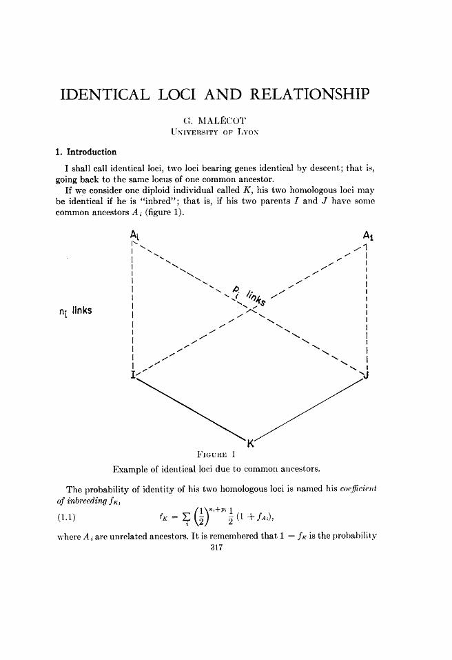
If we consider one diploid individual called K, his two homologous loci maybe identical if he is "inbred"; that is, if his two parents I and .1 have somecommon ancestors Ai (figure 1).

Al Al

ni links "

F'IG,URE 1

Example of idenitical loci due to commoni ancestors.

The probability of identity of his two homologous loci is named hlis coctJicie'itof inbreeding fK,

2 1

whiere Ai are unrelated ancestors. It is remembered that 1 - fK is the p)robalbility317

318 FIFTH BERKELEY SYMPOSIUM: MALE'COTof nonidentity; that is, the probability that the two homologous loci trace back,as far as we go back, to different ancestors. They are then "independent" in theprobabilistic sense; this means that they may or may not possess the same gene(a for instance), but knowing one of the two genes does not imply anythingabout the other. We call q the probability that a random locus bears the gene awith 1 - q = p being the overall probability of the other alleles grouped underthe symbol A. The independence of the two loci gives for the three genotypesaa, aA, AA, the probabilities q2, 2pq, and p2; whereas the identity of the twoloci gives the probabilities q, 0, p. So the a priori probabilities that a randomindividual K bears either of the three genotypes are(1.2) P = (1 -fK)q2 + fKq, 2Q = 2(1 -fK)pq, R = (1 -fK)p2 + fKp.The probabilities of the homozygotes are, in case of inbreeding, greater than incases of random mating. The probabilities (and then, in general, the frequencies)of heterozygotes, are decreased by random mating. The variance of a quan-titative character increases by inbreeding when the gene effects are additive.Now we may define more generally the coefficient of kinship of the two individualsI and J. We shall define it in such a manner as to obtain, if they are parentsof an individual K, the coefficient of inbreeding of K. The coefficient of kinshipof I and J is the probability that one locus chosen at random among the twoloci of I, and one locus chosen at random among the two homologous loci of J,are identical. So, the coefficient of inbreeding of K is equal to the coefficient ofkinship of his parents I and J

(1.3) fK = fiJ.If we account for mutation, which can modify a locus transmitted from parentto child with probability u, we have

(1.4) fK = (1 -U)'fJand

(1.5) fii =_[1(1 - U)]n (1 +fAi).

2. Coefficient of kinship

In a natural population, the probability of two individuals I and J bearing,in randomly chosen homologous chromosomes, two identical loci decreases whentheir distance increases because the probability of common ancestors decreases.It is the phenomenon of isolation by distance, going up to racial unlikeness ifthe distance is so large that there are very few identical loci between I and J.It is possible to calculate, as a function of the distance between I and J, theircoefficient of kinship; that is, the probability for two randomly chosen loci ineach to be identical. This function is dependent on the migration law; that is,the probability law ruling the distance between the birthplace of the child andthe birthplace of his parents, called the parental distance, whereas the distance

IDENTICAL LOCI AND RELATIONSHIP 319

between the birthplace of the two parents of each individual will be calledmarital distance. We shall call x the parental distance from child to parent.This x is an oriented vector in the two dimensional plane, but the arrows will beomitted for typographical simplicity. The coordinates of x will be called xi andx2; points of the plane, locating positions of individuals will be called b, and soforth, with coordinates b1, b2, and so forth. The elementary area of location ofan individual will be called db1 db2 = db or if this is the birthplace of parent,dx1 dx2 = dx. The migration law, the probability law of parental distance, willbe characterized by the probability density t(xi, x2), the elementary probabilityt(xl, x2) dxl dx2 = t(x) dx for shortness, or the distribution L(x1, x2), with dL =4 dx in the continuous case.With the assumption of separate generations, let us consider two individuals

I and J, belonging to the same generation Fn, and separated by vectorial dis-tance y, with coordinates yi and Y2. Their coefficient of kinship will be calledfn(y); it is obviously related to the coefficient of kinship of previous generations.If we were allowed to suppose that the parents of I and J are always distinct,we would have

(2.1) 5°(y) = (1 - u)2 f °n.-(y + z - x)t(z)t(x) dz dx,where u is the mutation rate.

pi

z

x

0 I

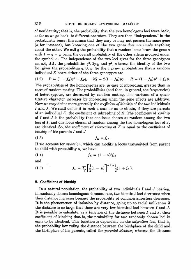
FIGURE 2

Distance between two individuals I and J, and theparents P, and PJ supplying the two loci.

But formula (2.1) does not account for the possibility that P, and Pi, theparents who supplied the two loci chosen in I and J, are the same individual,which is possible since the adults are in limited number. Indeed, PI and Pi maybe the same if they are born in the same elementary area dx, occupied by 6 dxindividuals, for which the corresponding probability is

(2.2) t(x) dxt(-y +x) dx,and if also they are the same, the probability of which is 1/6 dx. So, the prob-

320 FIFTH BERKELEY SYMPOSIUM: MALECOT

ability of P, and Pj being the same individual located at distance x from I is(2.3) f(x)f(x - y) dx/6.REMARK 1. The reasoning may also be used in the discontinuous case with

partition into separate groups of N individuals each, the probability of migra-tion from a group at vectorial distance d being 4(d), with d having discrete,perhaps entire, coordinates. The probability that the parents come from thesame group is then A(d)t(d - y), and the conditionlal probability that they arethe same is 1 divided by N. The probability of being the same individual locatedat distance d from I is then

(2.4) f(d)f(d - y)/N.When we tend to the case of a continuous distribution, we obtain formula (2.3).REMARK 2. In the previous reasoning, sex was not yet taken into account.

If we now suppose the densities of males and females are Al and 62 per unit area,the parents PI and PJ who have the randomly chosen loci of I and J may bothbe males (with probability 1/4) and identical with conditional probability oflocation(2.5) f(x)t(x - y) dx/bl,or they may both be females with probability 1/4 and identical with conditionialprobability of location(2.6) f(x)t(x - y) dx/&62.So formula (2.3) is valid if we put 1/46, + 1/462 = 1/6. If Al and 62 are equal,then 6 = 261, and is then total density; but in the general case a is only doublethe harmonic mean between 61 and 62.

2.1. Refinement of equation (2.1) to account for finiteness of population. Wehave to replace some infinitesimal terms of (2.1) corresponding to the samelocation of parents; that is, to the relation y + z = x and dz = dx. In cases ofprobability 1/6 dx, the coefficient of kinship p0n-1(0) of neighboring but distinctindividuals is to be replaced by the probability that two loci given to I and Jby the same parent PI were the same. This probability is 1/2 + fo/2, where fo isthe coefficient of inbreeding of Pi. So we have to add to formula (2.1) the cor-rective term

(2.7) (1 -u)2 f [2 (1 + fo) - Sn-1(0)] [t(x)f(x - y) dx]/6.We shall now put

(2.8) 1(1 +fo) -S'n-1(0)/6 = s"_- > 0

as a correction for the same )arent. We have inow to calculate the function so(x)and the constant sn_1 giving the coefficient of inbreeding fo, by solving equationsof wvhich one is the finlite difterenlce integral e(qutatioIn

(2.9) s°- (y) = (1 - u)2 f °ni-(Y + z - x)t(z)t(x) dzdx

+ (1 -')2 sn-_ f f(x)f(x - y) dx.


It is easy to see that, because the factor (1 - u)2 is less than one, the function5°nf(y) tends to a limit (p(y) as n tends to infinity. If we call s the limit of sn-1;that is, if we put

(2.10) 1 + fn- 2p(0)

anld if we put, for simplicity,(2.11) (1 - u)t(x) = g(x)giving us

(2.12) f g(x) dx = (1-u)(instead of f t(x) dx = 1), we now have to solve

(2.13) s(y) = f so(y + z - x)g(z)g(x) dz dx + s J g(x)g(x - y) dx.

The convolutions in (2.13) will be replaced by algebraic multiplications if weintroduce the following bidimensional Fourier transforms (where v is an arbitraryvector of coordinates vi and V2):

(2.14) G(v) J eivxg(x) dx (vectorial form)

fJ ei(vX+V.2)g(xi, x2) dxl dX2, (scalar form)

(2.1;) K(v) ff eivy(y) dy = f ei(VIYI+V22)1(yi, Y2) dy1 dy2-

By multiplying each member of (2.13) by(2.16) eivV = eiv(y+z-x)e-ivzeivz = eivxe-iv(x-)and integrating with respect to y, we obtain the formula(2.17) K(v) = K(v)G(-v)G(v) + sG(v)G(-v)which gives

(2.18) K(v) 1 -G(v)G(-v)Then the inversion of Fourier transform (2.15) gives

(2.19) so(y) = 1e-ivJ K(v) dv (vectorial form),

I42 f e-i(vY1+vl2Y2)K(vi, v2) dvi dv2 (scalar form).

These formulas may be simplified in the isotropic case where the migrationlaw, defined by 4(x1, x2), or by g(xI, x2) = (1 -u)t(x1, x2), is only dependent onthe absolute value, or "norm" of vector x; that is, (x1 + x2)1I2 = r.We then have, putting xi = r cos 0 and x2 = r sin 0,

(2.20) t(xI, x2) dxl dx2 = 4(r)r dr dO.


G(v) given by (2.14) is then dependent only on the norm lvl = (t, ±v+!)1/2,and is then known to be the "Hankel transform"

(2.21) G(|v|) = 27r(l -u) f| +

Jo(rjvj)rf(r) dr.

We use the notation G(lvI) to indicate a function depending only oIn the normlvi of vector v: and we shall henceforth omit the sign and write only G(v).The same can be said about equation (2.15), which gives the Hankel transform

of the coefficient of kinship so(Yl, Y2). But it is better to use the inverse transform(2.19) thus putting (y2 + y2)1/2 = a, sp(y) = p(a), and K(vi, V2) = K(Ivl) = K(v)the value of K(v) being given by (2.18).Then we may write

(2.22) (a) = J vJo(ajvj)K(v) dv.

Combining formulas (2.18), (2.21) and (2.22), we have

(2.23) G(v) (1 - u) f0 Jo(rv)27rrf(r) dr

s+ ' ~~G2(v)(2.24) sp(a) = vJo(av) 1 - G2(v) dv,

formulas which express the coefficient of kinship of I and J as a function oftheir distance a, in the stationary case, provided we know the migration lawdefined by the probability density 27rrtf(r) of the parental distance r (that is,the distance between parent and child).REMARK. Another interpretation is that, in the present isotropic case

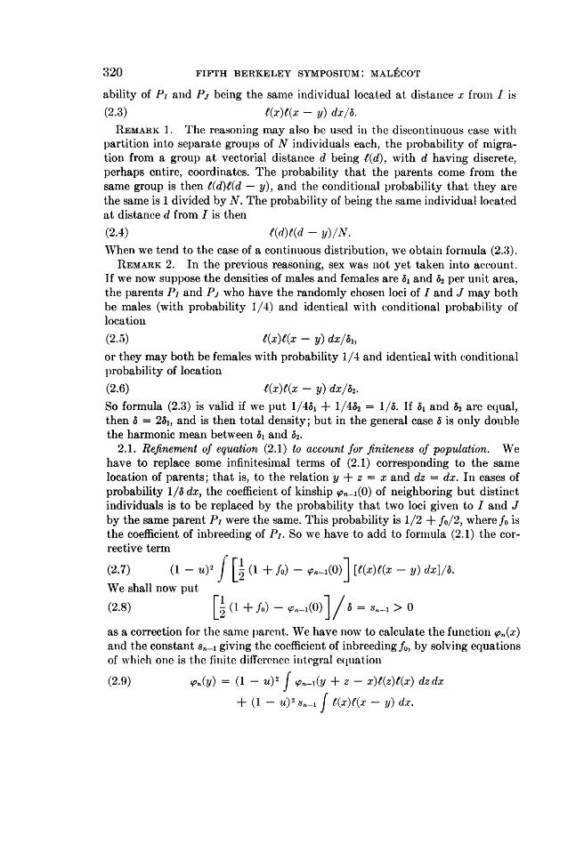
G2(jvl) = G(v)G(-v) is, apart from the factor (1 - u)2, the Fourier transform--* ---

of the difference of two independent vectors x and z, each having as probabilitylaw the migration law; so, in the case of complete random mating, G2 (v) is the

,~~~~~~~~~~FIGURE 3

Interpretation as the difference of two indepeindent vectors.


bidimensional Fourier transform of the vectorial marital distance, or the Hankeltransform of the absolute marital distance; then the distribution of maritaldistance may be introduced directly in (2.24). We put

(2.25) M(v) = (1 - u)2 f0f Jo(rv)m(r) dr,where m(r) is the probability density of the marital distance, and M(v) is,when v increases from zero, a decreasing function with the initial value M(O) =(1 - u)2. Then we have

(2.26) sp(a) = f 1 -M(v) Jo(av)v dv.

3. Application to a normal migration law

If, for the marital distance, m(r) is normal (the distribution of the parentaldistance is then itself normal, in case of complete random mating), we haveM(v) = (1 -U)2 exp (-o-2v2/4), where a2 is the second moment of the maritaldistance and

=sf (1 -~U)2 exp (- 0i2v2/4)(3.1) ip(a)-UV

Joavdv27rJo 1 (1 - u)2exp(-o2 /4) Jo(av)vdv,which gives by way of an easy integration

(3.2) .o(O) = log [1 - (1 -U)2] -2 log

Recall that s is related to so(O); see the last paragraphs. In case of "completerandom mating" wherefo = so(O), we get ([1], p. 59)

(3.3) s(O) = fo = [1 ± 2rra2/loguTo obtain an asymptotic expression of sp(a) when a is large, we shall use,

taking account of the smallness of the mutation rate, the asymptotic propertiesof the Fourier-Hankel transform. From (2.26) we see that p(a) is (apart fromthe factor s/27r) the transform of M(v)/[l - M(v)] which, in the vicinity ofv = 0, is very large, equivalent to 1/2u; and then decreases quickly from 1/2uto zero (when v increases); the principal part of V(a) for a large is given by thefirst derivatives (for v = 0) of the function MA(v)/[1 - M(v)], which are alsothe first derivatives of

(3.4) (1 -u)2(l - u2v2/4) 11 - (1 -u)2(1 - a2v2/4) 2u + a20,2/4

The Hankel transform of order zero of (M2 + v2)-' is Ko(am) ([2], p. 282), anidthus we obtain

(3.5) (p(a) - 2sT2 Ko [ (8u)1/2]


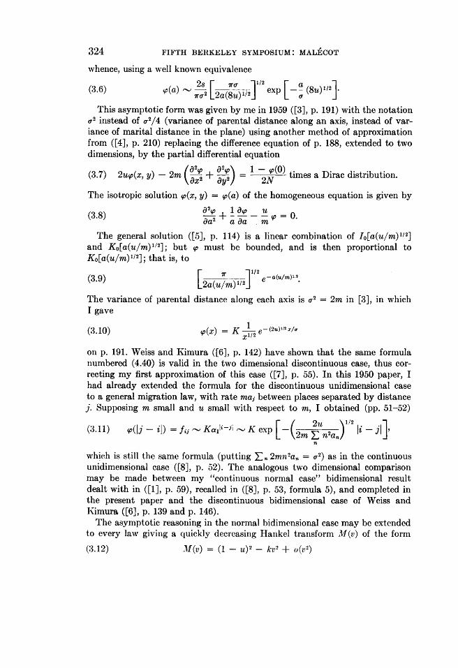
whence, usiing a well known equivalence

(3.6) ip(a) - r [2a(8u)1/2 exp [- (8u) 1/2].

This asymptotic form was given by me in 1959 ([3], p. 191) with the notationa2 instead of a2/4 (variance of parental distance along an axis, instead of var-iance of marital distance in the plane) using another method of approximationfrom ([4], p. 210) replacing the difference equation of p. 188, extended to twodimensions, by the partial differential equation

3x2m o2 2S\ 1 - °(0) times a Dirac distribution.

\ OX2 09y2/ 2NThe isotropic solution p(x, y) = (p(a) of the homogeneous equation is given by

(3.8) 92S0+ 1 49 _ = 0.aa2d aaa .mThe general solution ([5], p. 114) is a linear combination of Io[a(u/m) 1/2]

and Ko[a(u/m) 1/2]; but so must be bounded, and is then proportional toKo[a(u/m) 1/2]; that is, to

(3.9) [2a(u/m) 1/2]1 e

The variance of l)arental distance along each axis is C2 = 2m in [3], in whichI gave

(3.10) so(x) = K 1 e-(2u) I/'

on p. 191. Weiss and Kimura ([6], p. 142) have shown that the same formulanumbered (4.40) is valid in the two dimensional discontinuous case, thus cor-recting my first approximation of this case ([7], p. 55). In this 1950 paper, Ihad already extended the formula for the discontinuous unidimensional caseto a general migration law, with rate maj between places separated by distance.j. Supposing m small and u small with respect to m, I obtained (pp. 51-52)

(3.11) o(fj - ij) = fij- Kalli-i '- K exp [( 2m 1En2an)I Ain

which is still the same formula (putting E,, 2mn2a,, a=2) as in the continuousunidimensional case ([8], p. 52). The analogous two dimensional comparisonmay be made between my "continuous normal case" bidimensional resultdealt with in ([1], p. 59), recalled in ([8], p. 53, formula 5), and completed inthe present paper and the discontinuous bidimensional case of Weiss andKimura ([6], p. 139 and p. 146).The asymptotic reasoning in the normal bidimensional case may be extended

to every law giving a quickly decreasin, Hankel transform M(v) of the form

(3.12) M(v) = (1 - u)2 - kv2 + o(v2)


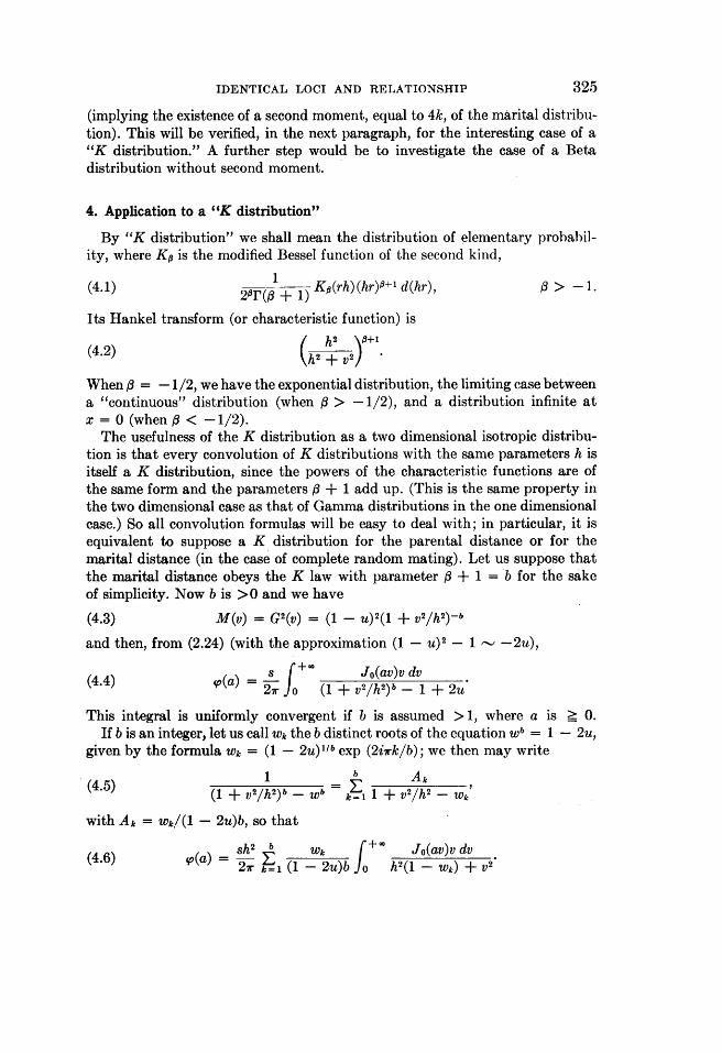
(implying the existence of a second moment, equal to 4k, of the marital distribu-tion). This will be verified, in the next paragraph, for the interesting case of a"K distribution." A further step would be to investigate the case of a Betadistribution without second moment.

4. Application to a "K distribution"

By "K distribution" we shall mean the distribution of elementary probabil-ity, where Kg is the modified Bessel function of the second kind,

(4.1) 2F( + 1) Kg(rh)(hr)0+1 d(hr), f> -1.

Its Hankel transform (or characteristic function) is

(4.2) (h2 + v2)When i3 =-1/2, we have the exponential distribution, the limiting case betweena "continuous" distribution (when A > -1/2), and a distribution infinite atx = 0 (when ; < -1/2).The usefulness of the K distribution as a two dimensional isotropic distribu-

tion is that every convolution of K distributions with the same parameters h isitself a K distribution, since the powers of the characteristic functions are ofthe same form and the parameters 3 + 1 add up. (This is the same property inthe two dimensional case as that of Gamma distributions in the one dimensionalcase.) So all convolution formulas will be easy to deal with; in particular, it isequivalent to suppose a K distribution for the parental distance or for themarital distance (in the case of complete random mating). Let us suppose thatthe marital distance obeys the K law with parameter d + 1 = b for the sakeof simplicity. Now b is >0 and we have

(4.3) M(v) = G2(v) = (1-u)2(1 + v2/h2ftband then, from (2.24) (with the approximation (1 - U)2 - 2u),

(4.4) ~ (a) = _3 Jo(av)v dv2rJo (1 + v2/h2)b -1 + 2u

This integral is uniformly convergent if b is assumed >1, where a is _ 0.If b is an integer, let us call Wk the b distinct roots of the equation Wb = 1 - 2u,

given by the formula Wk = (1 - 2u)l/b exp (2irk/b); we then may write

(4.5) 1b A(1 + v2/2)b b =1 1 2/h k

with Ak = wk/(l- 2u)b, so that

(4.6) 27r k-1 (-h2b WokC -Jo(av)v dv27ak= 1(I--(2u)b J h2(1 Wk)+v

326 FIFTH BERKELEY SYMPOSIUM: MALUCOT

Each integral is easily calculated by the formula

(47) f+Jo(av)vdv=Ko(am);

see Guelfand and Chilov ([2], p. 282) which givessh2 b Wk(4.8) (a) = k (1 - 2u)b Ko[ah(1 - Wk)12].

The expression (1 -w)112 may be chosen with an argument between -7/4and +7r/4.

If a is large, this sum Eb- contains a term much larger than the others;indeed, the root Wb = (1 - 2u)lIb _ 1 -2u/b is (if b is not large), muchnearer 1 than the others, making the corresponding value of IKol much largerthan the others (the real part and the modulus of ah(1-Wb))1/2 being muchless than those of ah(l - Wk)1I2 if k # b). Therefore,(4.9)~~~(a) h2 r2s(4.9) s o(a) - 8KO[ah(2u/b)12] = Ko[a(8u/M2)"12].

(The second moment M2 is 4b/h2.)The analyticity of (2.24) with respect to b > 1 ensures validity even when

b > 1 is not an integer. Then we may apply the approximation(4.10) s~~~~~h2[ 7r 11/2 2/)2L2rb[2ah(2u/b) 12

2s F 7rM21/2I/2 e-a(8u/M2)112WM2 L2a(8u)I/2J

which is the same as in the case of the normal law.For a = 0, formula (2.24) gives directly

h2+. d(l + V2/h2)(4.11) ,p(0) = sh2 (1+v2/h2)b1+2u

sh2 [+ dz4 f zb - 1 + 2u

which is convergent only if b > 1. In the vicinity of z = 1, we now write

zb= 1 + W, bz6-- dz = dw,(4.12) A2 dw

'P(0) -s2Id47rb Jo (2u + w)(1 + w)(1)/Because u is small this incomplete B integral is equivalent to

1dw _(4.13) lo _-log (2u) = logJo2u+w 2u o2uWhen so(O) = fo, which is the case of completely random mating, we have, byreplacing s with [1 - (p(O)]/26, and 4b/h2 with the second moment M2, therelation


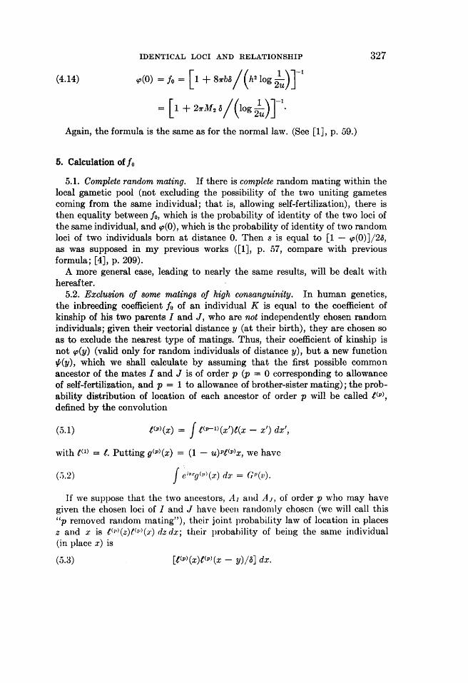
(4.14) s(°) = fo =[A+ Sr/(h2 log2u)= [1 + 27rM2 5/(log 2 )]

Again, the formula is the same as for the normal law. (See [1], p. 59.)

5. Calculation of fo

5.1. Complete random mating. If there is complete random mating within thelocal gametic pool (not excluding the possibility of the two uniting gametescoming from the same individual; that is, allowing self-fertilization), there isthen equality between fo, which is the probability of identity of the two loci ofthe same individual, and so(0), which is the probability of identity of two randomloci of two individuals born at distance 0. Then s is equal to [1 - (0)]/2B,as was supposed in my previous works ([1], p. 57, compare with previousformula; [4], p. 209).A more general case, leading to nearly the same results, will be dealt with

hereafter.5.2. Exclusion of some matings of high consanguinity. In human genetics,

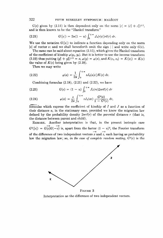
the inbreeding coefficient fo of an individual K is equal to the coefficient ofkinship of his two parents I and J, who are not independently chosen randomindividuals; given their vectorial distance y (at their birth), they are chosen soas to exclude the nearest type of matings. Thus, their coefficient of kinship isnot so(y) (valid only for random individuals of distance y), but a new function+p(y), which we shall calculate by assuming that the first possible commonancestor of the mates I and J is of order p (p = 0 corresponding to allowanceof self-fertilization, and p = 1 to allowance of brother-sister mating); the prob-ability distribution of location of each ancestor of order p will be called t(P),defined by the convolution

(5.1) t(P) (x) = J t(-')(x')t(x - x') dx',

with ((l) = t. Putting g(P)(x) = (1 - u)P&t()x, we have

(5.2) eixg(P)(x) dx = Gp(v).

If we suppose that the two ancestors, Al and Ai, of order p who may havegiven the chosen loci of I and J have been randomly chosen (we will call this"p removed random mating"), their joint 1)robability law of location in placesz and x is V(7)(z)f(P)(x) dz dx; their probability of being the same ilndividual(in place x) is

(5.3) [t(P)(x)tP)(x - y)/6] dx.


AI A

p /

links

\ /I

\ //

\ /

y /

FIGuRE 4

Determination of joint probability law of location of two anicestors,and of the probability of their being the same individual.

So 4#(y) is given by

(5.4) -P(y) =f po(y + z - x)g(P)(z)g'P)(x) dz dx + S gv(x)gc( ~d

with, as before,

(5.5) 8 = [ +fo P0]Compare (5.4) to (2.13).The Fourier transform gives

(5.6) H(v) =ff ei-4'(y) dy = K(v)[G(v)]2p + 8[G(v)]2P

- [l (v) +is]2p(v) = ___using (2.18).

Hence,

(5.7) 4p(y) = ffe-i-H(v) dv J= 1 J 1(JJ)vJdlvi.It is nlow possible to calculate fo. If we suppose we kniow the bidimensional


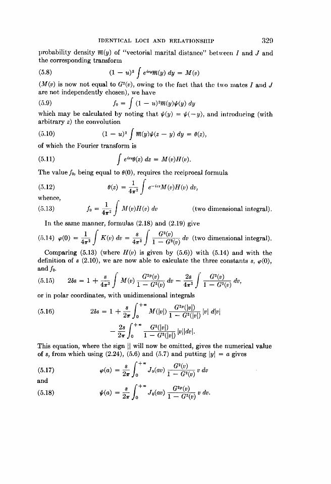
probability density m(y) of "vectorial marital distance" between I and J andthe corresponding transform

(5.8) (1 - U)2 f eivym(y) dy = M(v)

(M(v) is now not equal to G2(v), owing to the fact that thc two mates I and Jare not independently chosen), we have

(5.9) fo = f (1 - u) 2m(y) p(y) dywhich may be calculated by noting that ,6(y) = ,6(-y), and introducing (witharbitrary z) the convolution

(5.10) (1 - u)2 J m(y)P(z - y) dy = 0(z),of which the Fourier transform is

(5.11) f eivzo(z) dz = M(v)H(v).

The value fo, being equal to 0(0), requires the reciprocal formula

(5.12) 0(z) = 41r2 J e-itzM(v)H(v) dv,whence,(5.13) fo = 42 fAl (v)H(v) dv (two dimensional integral).

In the same manner, formulas (2.18) and (2.19) give

(5.14) so(°) = 412 f K(v) dv = 4 1 G2(V) dv (two dimensional integral).Comparing (5.13) (where H(v) is given by (5.6)) with (5.14) and with the

definition of s (2.10), we are now able to calculate the three constants s, so(O),and fo.

(5.15) 26s = 1 + 4S M(v) G2p(V) dv-d2 G2(V)4;:i 1 - G2(V) 47r2 1 - G2(V)

or in polar coordinates, with unidimensional integrals

(5.16) 26s = 1+ 1M(-v)1 G2p(IvI) lvl dlvj27rJ 1 G2 Iv) v28+ G2(~~~IVI vl ldvl!27rJ 1 -..G2 (lVI)

This equation, where the sign II will now be omitted, gives the numerical valueof s, from which using (2.24), (5.6) and (5.7) and putting jyI = a gives

r ~~~G2(V)(5.17) p(a) = J Jo(av) v dv2j Jav 1- G2(v) Vdand

(5.18) 4t'(a) = GJ Jo(av) G2p(V) v dv.J- Jav 1- G2(V)


5.3. Numerical results. We have

(5.19) [s + = 2G2(V) +2I(V)G2)(v) v dv]

G'(v(5.20) so(°) =

s J _ v dv,

(5.21) C(0) = J> v dv,and, by (5.13),

(5.22) fo= .11() -1--G v dv.

5.4. Particular case: K distributions. All the formulas are easy to work outif the parental distance and the marital distance are "K distributed," theHankel transform for law of parental distance being

(5.23) G(v) = (1-u) (1+ )

For simplicity let us put G2(v) = M(v). (Accounting for nonrandomness ofmating could be done by taking for m(r) a K distribution with a parameterdifferent from b, but this correction has a small effect on formulas (5.19) and(5.22)). We then have

(5.24) G2 = (1- u)2 1 + V2b

The calculation of the integral in (5.21) is easy and gives the integrals in(5.20) and (5.22) (with M(v) = G2(v)). All integrals are convergent if b is sup-posed > 1. Let us write

(5.25) I, =JG2v dv

J)p+ (1 + v2Ih2)-bp V

lou2 1- (1- u)2(1 + v2/h2)-b (2)which, putting z = 1 + v2/h2, is

(5.26) (1 - z-bp dz,)2v--j 1 -(1 - U)2Zb

or, again puttingzb = 1 + wetbzb-l dz = dw.

(5.27) h2 + (1+ W)-P+l/bI,, = (1-u)2J2b 1 + -(1-)2 d

The two equations (5.20) and (5.22) then give, jointly with the relation2sb = 1 +fo -2so(),


(5.28) 2sa = 1 + (Ip+l - 2II)

,2psh2 f - (1 ± w)-lP+1/b - 2(1 +W-+l=1+(1U)2P2b Jo 1- (1-U)2 + W

The rapid increase of the denominator from the very small initial value1 - (1 - U)2 2u allows us to replace the integral by the approximation

1 _ 1 r1(5.29) f 1+w dw =- log (2u +w) - log 2u.

Replacing (1 -u)2P by 1 (since p is not very large) and 4b/h2 by M2, we obtainS o u s.'2 log (1/2u) 1(5.30) 2so-1 -MrM2 log 2U, S[ 20+ rM2]

which is a particular case of formula (5.19). Then

(5.31) f 2=2

IP+ and s(°)=2

I,;

or I,+i and I, are, by the same reasoning, equivalent to

(5.32) 1 dw )log(-

We then have

(5.33) fo - S°(0) irM log (2) i [1 + 27rM2/log1This differs very little from the case of complete random mating.

In the case of a normal law, the result would be the same (and also in the caseof other laws of finite second moment M2). It remains to investigate the caseof migration laws without a second moment.

I am grateful to the Berkeley Symposium and to the Universities of Hawaii,Stanford, and Michigan State for the help they offered to me by their kindinvitation to discuss this paper in their lectures or seminars.

REFERENCES

[1] G. MALACOT, Les Mathematiques de l'Heredite, Vol. 1, Paris, Masson, 1948.[2] I. M. GUELFAND and G. E. CHILOv, Les Distributions, Vol. 1, Paris, Dunod, 1962 (French

translation of Russian Generalized Functions by I. M. Gel'fand and G. E. Shilov, Moscow,Fiz. Mat. Giz., 1959).

[3] G. MALACOT, "Les modeles stochastiques en genetique de population," Publ. Inst. Statist.Univ. Paris, Vol. 8 (1959), pp. 173-210.

[4] , "Migration et parent6 g6n6tique moyenne," Entretiens de Monaco en scienceshumaines, 1962, pp. 205-212.

[5] I. N. SNEDDON, Special Functions of Mathematical Physics and Chemistry, Edinburgh,Oliver and Boyd; New York, Interscience, 1956.

332 FIFTH BERKELEY SYMPOSIUM: AMALE'COT

[6] (G. 11. WI-EISS and M. KIMuRA, "A mlathematical analysis of the stepping stoiie model ofgenetic correlation," J. Appl. Probability, Vol. 2 (1965), pp. 129-149.

[7] G. MALUCOT, "Quelques schemas probabilit(s sur la variabilit6 des populations naturelles"Ann. Univ. Lyon, Sciences, Section A, Vol. 13 (1950), pp. 37-60.

[51] - , "The decrease of relationship with distance," Cold Spring harbor Symp. Quant.Biol., Vol. 20 (1955), pp. 52-53.

identical loci relationship - spotlight exhibits...

Documents