identification and investigation of new low-dimensional ... · identification and investigation of...
TRANSCRIPT
Loughborough UniversityInstitutional Repository
Identification andinvestigation of new
low-dimensional quantumspin systems
This item was submitted to Loughborough University's Institutional Repositoryby the/an author.
Additional Information:
• A Doctoral Thesis. Submitted in partial fulfillment of the requirementsfor the award of Doctor of Philosophy of Loughborough University.
Metadata Record: https://dspace.lboro.ac.uk/2134/8963
Publisher: c© J. M. Law
Please cite the published version.

This item was submitted to Loughborough’s Institutional Repository (https://dspace.lboro.ac.uk/) by the author and is made available under the
following Creative Commons Licence conditions.
For the full text of this licence, please go to: http://creativecommons.org/licenses/by-nc-nd/2.5/

Identification and investigation of
new low-dimensional quantum spin
systems
by
Joseph M. Law
Doctoral Thesis
Submitted in partial fulfillment of the requirements for the award of
Doctor of Philosophy of Loughborough University
September 27, 2011
c⃝ by J. M. Law 2011
Hwæt!
Beowulf - Unknown author
circa 8th-11th century
i

Abstract
This thesis focuses on one area of modern condensed matter physics,
namely low-dimensional magnetism, and more specifically one-dimen-
sional linear chains. The work herein can be split into three parts. The
first part provides a tool for the greater community. I herein propose a
Pade approximation for the temperature dependent magnetic suscepti-
bility of a S = 3/2 spin chain, that is more accurate than those already
known. The approximation allows one to fit experimentally measured
magnetic susceptibilities and ascertain values such as the near-neighbour
spin exchange interaction and the g-factor. The second and third parts
of this thesis are both concerned with experimentally and theoretically
characterizing two isostructural linear S = 1/2 chain compounds on op-
posite ends of the 3d transition metal series. The compounds, CuCrO4
(3d9) and TiPO4 (3d1), are shown to have completely different ground
states despite both being largely isostructural and S = 1/2 quantum
spin systems. In this work and the resulting publications it is shown that
CuCrO4 is a one-dimensional S = 1/2 spin chain with anti-ferromagnetic
nearest- and next nearest-neighbour spin exchange interactions. The
ratio of these spin exchange interactions is shown experimentally and
theoretically to be approximately 2, putting CuCrO4 in the vicinity of
the Majumdar-Ghosh point, for which the magnetic ground-state can
ii

be solved analytically. Small ferromagnetic inter-chain coupling leads
to long-range ferromagnetic ordering between anti-ferromagnetic chains
at 8.2(2) K. At this temperature a spontaneous electrical polarization
is observed. This classifies CuCrO4 as a type-II multiferroic. Contrary
to CuCrO4, TiPO4 has a non-magnetic ground state. At 111 and 74 K
TiPO4 undergoes a two stage phase transition, which is interpreted as
a spin-Peierls transition. There is evidence that below 74 K TiPO4 has
a new crystal structure, in which there are alternating dimerised chains
and two different PO4 tetrahedral units. Currently the new structure
has not been identified and no super-structure reflections have been con-
firmed in either low-temperature neutron or x-ray diffraction.
In summary this thesis presents some experimental and theoretical con-
tributions to the field of low-dimensional magnetism.
iii

Publication list
1. J. M. Law, C. Hoch, M.-H. Whangbo, and R. K. Kremer, Descrip-
tion of anhydrous (black) dioptase as a S=1/2 uniform antiferro-
magnetic chain system, Zeitschrift fur anorganische und allgemeine
Chemie 636, 54 (2010).
2. J. S. Kim, S. H. Khim, H. J. Kim, M. J. Eom, J. M. Law, R.
K. Kremer, J. H. Shim, and K. H. Kim, Electron-hole asymmetry
revealed in the phase diagrams of Fe-site doped SrFe2As2, Phys.
Rev. B 82, 024510 (2010).
3. M. Mourigal, M. Enderle, R. K. Kremer, J. M. Law and B. Fak,
Ferroelectricity from spin supercurrents in LiCuVO4, Phys. Rev. B
83, 100409(R) (2011).
4. J. M. Law, C. Hoch, R. Glaum, I. Heinmaa, R. Stern, J. Kang, C.
Lee, M.-H. Whangbo, and R. K. Kremer, Spin-Peierls transition in
the S=1/2 compound TiPO4 featuring large intrachain coupling,
Phys. Rev. B 83, 180414(R) (2011).
5. A. Bussmann-Holder, J. Kohler, R. K. Kremer, and J. M. Law,
Analogies of structural instabilities in EuTiO3 and SrTiO3, Phys.
Rev. B 83, 212102 (2011).
iv

6. J. M. Law, P. Reuvekamp, R. Glaum, C. Lee, J. Kang, M.-H.
Whangbo, and R. K. Kremer, Quasi-one-dimensional antiferromag-
netism and multiferroicity in CuCrO4, Phys. Rev. B 84, 014426
(2011).
7. M. Johnsson, P. Lemmens, J. M. Law, R. K. Kremer, M.-H. Whangbo
and K. Y. Choi, Structural and Magnetic Properties of FeTe3O7X
(X=Cl, Br), in preparation, (2011).
v
Contents
1 Magnetism 1
1.1 Magnetism . . . . . . . . . . . . . . . . . . . . . . . . . . 1
1.1.1 The magnetic moment . . . . . . . . . . . . . . . 2
1.1.2 Crystal electric field . . . . . . . . . . . . . . . . 4
1.1.3 Interactions . . . . . . . . . . . . . . . . . . . . . 6
1.1.4 Spin models . . . . . . . . . . . . . . . . . . . . . 9
1.2 One-dimensional magnetism . . . . . . . . . . . . . . . . 10
1.2.1 Multiferroicity . . . . . . . . . . . . . . . . . . . . 13
1.2.2 Some known low-dimensional S = 1/2 quantum
spin chains . . . . . . . . . . . . . . . . . . . . . . 14
1.2.3 Inter-chain couplings and long-range ordering . . 21
vi

1.2.4 Electron paramagnetic resonance theory . . . . . 22
1.2.5 Pade approximation for the molar magnetic sus-
ceptibility of a S = 32 Heisenberg quantum anti-
ferromagnetic spin chain . . . . . . . . . . . . . . 25
1.3 Summary . . . . . . . . . . . . . . . . . . . . . . . . . . 32
2 Experimental methodology and computation 33
2.1 X-ray and neutron diffraction . . . . . . . . . . . . . . . 34
2.1.1 Single crystal diffraction . . . . . . . . . . . . . . 34
2.1.2 Powder diffraction . . . . . . . . . . . . . . . . . 34
2.2 Magnetisation . . . . . . . . . . . . . . . . . . . . . . . . 36
2.2.1 SQUID magnetometry . . . . . . . . . . . . . . . 36
2.3 Specific heat . . . . . . . . . . . . . . . . . . . . . . . . . 40
2.3.1 Relaxation calorimetry . . . . . . . . . . . . . . . 40
2.3.2 Adiabatic Nernst calorimeter . . . . . . . . . . . 41
2.4 Electron Paramagnetic Resonance spectroscopy . . . . . 42
2.5 Dielectric capacitance . . . . . . . . . . . . . . . . . . . . 45
2.6 Computation . . . . . . . . . . . . . . . . . . . . . . . . 46
vii

2.6.1 Algorithms and Libraries for Physics Simulations
- ALPS . . . . . . . . . . . . . . . . . . . . . . . 46
2.7 Summary . . . . . . . . . . . . . . . . . . . . . . . . . . 47
3 CuCrO4 - A new multiferroic material 48
3.1 Crystal structure . . . . . . . . . . . . . . . . . . . . . . 49
3.2 Sample preparation . . . . . . . . . . . . . . . . . . . . . 50
3.3 Magnetic susceptibility . . . . . . . . . . . . . . . . . . . 52
3.4 Specific heat . . . . . . . . . . . . . . . . . . . . . . . . . 60
3.5 Electron paramagnetic resonance . . . . . . . . . . . . . 66
3.6 ab initio calculations . . . . . . . . . . . . . . . . . . . . 72
3.7 Dielectric capacitance . . . . . . . . . . . . . . . . . . . . 77
3.8 Discussion and conclusion . . . . . . . . . . . . . . . . . 81
3.9 Summary . . . . . . . . . . . . . . . . . . . . . . . . . . 83
4 TiPO4 - A new spin-Peierls system? 85
4.1 Introduction and crystal structure . . . . . . . . . . . . . 85
4.2 Sample preparation . . . . . . . . . . . . . . . . . . . . . 88
viii

4.3 Magnetic susceptibility . . . . . . . . . . . . . . . . . . . 89
4.4 Specific heat . . . . . . . . . . . . . . . . . . . . . . . . . 95
4.5 Electron paramagnetic resonance . . . . . . . . . . . . . 97
4.6 ab initio calculations . . . . . . . . . . . . . . . . . . . . 104
4.7 Magic angle spinning 31P nuclear magnetic resonance and
Raman spectroscopy measurements . . . . . . . . . . . . 109
4.8 Low-temperature diffraction . . . . . . . . . . . . . . . . 117
4.9 Discussion and conclusion . . . . . . . . . . . . . . . . . 124
4.10 Summary . . . . . . . . . . . . . . . . . . . . . . . . . . 127
5 Conclusion 128
ix
List of Figures
1.1 Taken from magnetism and magnetic materials by J. M.
D. Coey (a): The five orbitals of the 3d transition metals.
(b): The energy splitting of the 3d orbitals (from left to
right); a free atom, an atom in a triangular based pyra-
mid environment, an atom in a non-distorted octahedral
environment and an atom in a cubic environment. (c):
The energy landscape of the 3d orbitals in an elongated
(left) and a compressed (right) octahedral environment. 5
1.2 A pictorial representation of the high- and low-spin con-
figurations for Fe3+. . . . . . . . . . . . . . . . . . . . . . 6
1.3 A graphical representation of the radial wave functions of
the free, bonded and anti-bonded states of the H2 molecule.
Taken from Magnetism in Condensed Matter Physics by
S. Blundell. . . . . . . . . . . . . . . . . . . . . . . . . . 7
x
1.4 A simplified one-dimensional chain of atoms, with the nn
and nnn spin exchange interactions indicated. . . . . . . 11
1.5 A pictorial representation of a frustration in one-dimensional
lattice. . . . . . . . . . . . . . . . . . . . . . . . . . . . . 12
1.6 The magnetic susceptibility of a uniform nn Heisenberg
spin chain with Jnn = 1 and a g-factor = 2, calculated
using the Pade approximation put forth by Johnston et al.. 13
1.7 The nn nnn spin exchange phase diagram for S = 1/2
one-dimensional system, adapted from Bursill et al.. The
coloured sections/lines are density functional theory cal-
culations for real systems, except the line labeled LiCuVO4
INS which is based on an inelastic neutron scattering results. 16
1.8 Main (o): The relative dielectric constant of LiCuVO4 ver-
sus temperature. Inset (o): The electrical polarization of
LiCuVO4, calculated from the pyroelectric current, versus
temperature. Taken from Schrettle et al.. . . . . . . . . . 17
1.9 Main (o): The molar magnetic susceptibility of CuCl2
measured in a magnetic field of 1 T versus temperature.
Inset (o): A log-log plot of the specific heat of CuCl2
versus temperature. All results taken from Banks et al.. . 19
xi
1.10 Main (o): The relative dielectric constant of CuCl2 versus
temperature, for various magnetic fields. Inset (o): The
electrical polarization of CuCl2, calculated from the py-
roelectric current, versus temperature. Taken from Seki
et al.. . . . . . . . . . . . . . . . . . . . . . . . . . . . . 20
1.11 The electron paramagnetic resonance normalised linewidth
versus reduced temperature for CuGeO3, KCuF3 and NaV2O5
shown against a linear line. The graph is taken from the
work by Oshikawa and Affleck. . . . . . . . . . . . . . . . 23
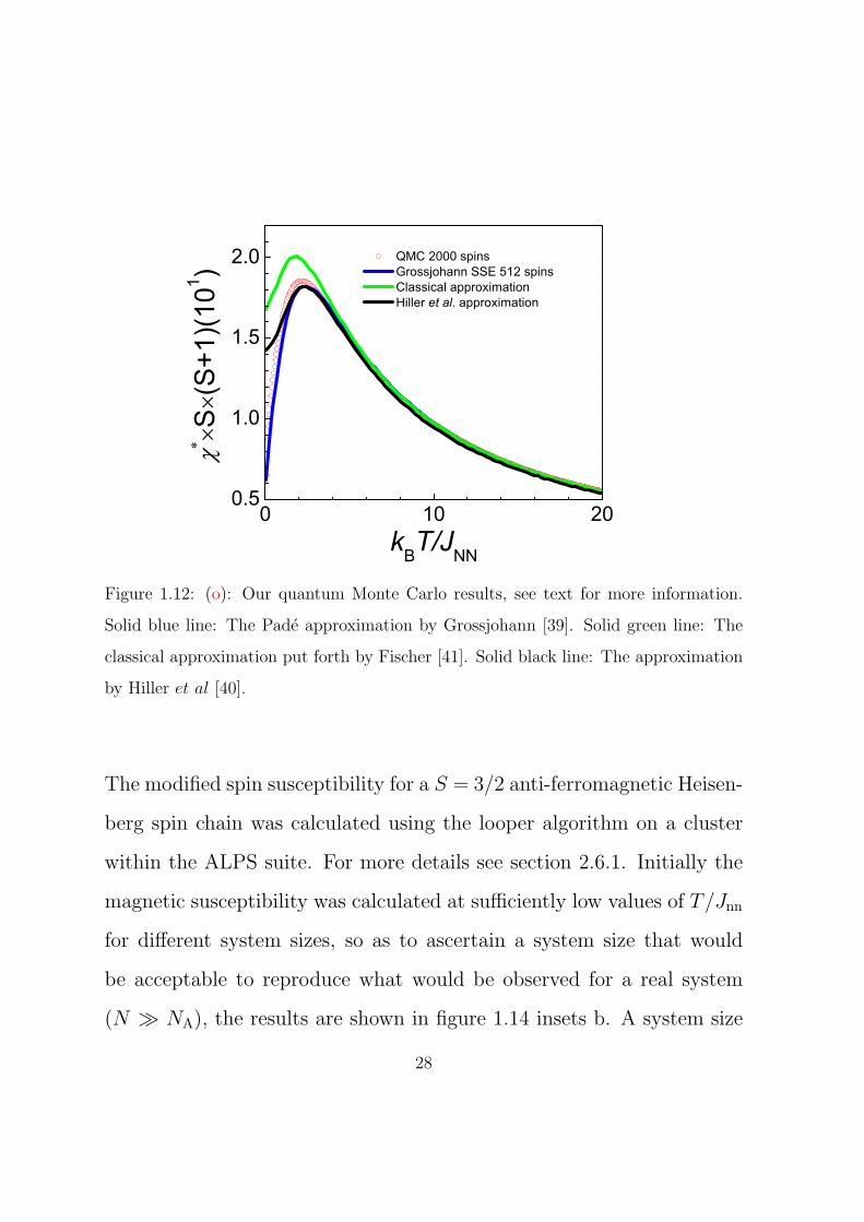
1.12 (o): Our quantum Monte Carlo results, see text for more
information. Solid blue line: The Pade approximation by
Grossjohann. Solid green line: The classical approxima-
tion put forth by Fischer. Solid black line: The approxi-
mation by Hiller et al. . . . . . . . . . . . . . . . . . . . 28
1.13 Left: The scaled computation time versus system size at a
reduced temperature of 0.05. Right: The arbitrary com-
putation time versus spin, at a reduced temperature of
0.05. . . . . . . . . . . . . . . . . . . . . . . . . . . . . . 29
xii

1.14 Main: (o): The temperature dependent modified spin sus-
ceptibility for a S = 3/2 spin chain with nn spin exchange
interactions, calculated by quantum Monte Carlo using
the ALPS suite, versus reduced temperature. Solid red
line: A fit to a Pade approximation as discussed in the
text. (a): (o): The difference between the modified spin
susceptibility as calculated by quantum Monte Carlo and
the Pade approximation fitted to the simulation. The
solid red lines denotes the boundaries of the error bars
given for the quantum Monte Carlo calculation. (b) The
modified spin susceptibility for different systems sizes at a
fixed reduced temperature of 0.05. N denotes the number
of spins. . . . . . . . . . . . . . . . . . . . . . . . . . . . 30
2.1 Schematic of the powder diffractometer HRPT at the Paul
Scherrer Institute (Switzerland). . . . . . . . . . . . . . . 36
2.2 Left: A filled gelatine capsule as used for measuring the
magnetization. Right: A disassembled, empty, gelatine
capsule, prior to use for measuring magnetization. . . . . 38
xiii

2.3 Left: A filled and sealed quartz tube ready for magnetiza-
tion measurements. Right: A closer view of the seal half
way up the tube. . . . . . . . . . . . . . . . . . . . . . . 38
2.4 Top: An empty glass bell jar. Bottom: A full sealed glass
bell jar, ready for specific heat measurements; left is a
view from the top and right is a view from the side. . . . 42
2.5 Left: The electron paramagnetic resonance sample holder
with a mounted temperature sensor. Right: The electron
paramagnetic resonance neutral low-background suprasil c⃝
quartz tube with a sample mounted. . . . . . . . . . . . 43
3.1 The crystal structure of CuCrO4, projected slightly off of
the c-axis. The unit cell is doubled along the c-axis. Blue
octahedra: CuO6 units. Green tetrahedra: CrO4 units. . 49
xiv

3.2 (o): Measured x-ray powder diffraction pattern of CuCrO4
(λ = 0.70930 A ). Solid red line: Calculated pattern
(Rp = 13.1%, reduced χ2 = 1.15) using the parameters
given in table 3.1. Solid blue line: The offset difference
between measured and calculated patterns. The positions
of the Bragg reflections used to calculate the pattern are
marked by the green vertical bars in the lower part of the
figure. . . . . . . . . . . . . . . . . . . . . . . . . . . . . 52
3.3 The molar magnetic susceptibility of CuCrO4, in the low-
temperature regime, versus temperature for various mag-
netic fields. Red symbols: Heating data. Blue symbols:
Cooling data. . . . . . . . . . . . . . . . . . . . . . . . . 54
3.4 (o): The inverse molar magnetic susceptibility versus tem-
perature of CuCrO4, measured in a field of 7 T. Red solid
line: Fit to the modified Curie-Weiss law as given in equa-
tion 3.1. . . . . . . . . . . . . . . . . . . . . . . . . . . . 56
3.5 (o): The 7 T molar magnetic susceptibility versus tem-
perature for CuCrO4. Dashed/solid lines: The simulated
molar magnetic susceptibility for various cases, see text
for more details. . . . . . . . . . . . . . . . . . . . . . . . 57
xv
3.6 Full diagonalization results. Solid red and black lines are
the magnetisation and d(M)d(H) versus applied magnetic field,
respectively. . . . . . . . . . . . . . . . . . . . . . . . . . 60
3.7 The specific heat versus temperature for CuCrO4. (o):
0 T data. (△): 9 T data, offset by +0.5 J/molK. . . . . 62
3.8 (o): The specific heat divided by temperature versus tem-
perature for CuCrO4, in the temperature range of the
anomaly. . . . . . . . . . . . . . . . . . . . . . . . . . . . 63
3.9 The specific heat divided by T 3/2 versus T 3/2. (o): Mea-
sured data. Solid red line: linear fit, with a slope of
4.31(1) × 10−3 J/molK4 and an intercept of 0.0109(1)
J/molK5/2. . . . . . . . . . . . . . . . . . . . . . . . . . . 65
3.10 (o): Electron paramagnetic resonance signal for CuCrO4
taken at 297(1) K. Solid red line: Fit to equation 2.1. . . 67
3.11 Fitted parameters of the electron paramagnetic resonance
signal of CuCrO4 versus temperature. (a): Intensity of
the electron paramagnetic resonance signal. (b): g-factor.
(c): The half width at half maximum and the solid red
line is a fit to a linear slope, with a gradient of 2.75(2)
T/K and an intercept of -220(5) K. . . . . . . . . . . . . 70
xvi

3.12 (o): Fitted inverse of the integrated electron paramag-
netic resonance intensity of CuCrO4 versus temperature.
Solid red line: Linear fit with an arbitrary gradient and
an intercept of -63.1(1) K. . . . . . . . . . . . . . . . . . 71
3.13 (a): Spin exchange pathways used for the mapping for the
density functional theory results. (b): The five spin con-
figurations for which the total energy has been calculated
by GGA+U calculations. Shown are the equations used
from mapping the energies onto the aforementioned spin
exchange pathways. Shown below in parentheses are the
relative energies given in meV, first for U = 4 eV and then
for U = 6 eV. . . . . . . . . . . . . . . . . . . . . . . . . 74
3.14 The predicted magnetic structure of CuCrO4, the chemi-
cal unit cell is denoted by the dashed box. (a) The mag-
netic structure in the a-b plane, white and black circles
represent different magnetic moment directions. (b) The
magnetic structure within the a-c-plane, with the mag-
netic moments represented by an arrow. . . . . . . . . . 77
xvii
3.15 Main: The temperature dependence of the relative di-
electric constant for CuCrO4 at low-temperatures under
various magnetic fields, refer to legend. (a): A magnetic
isotherm of the relative dielectric constant at 5.2(1) K.
(b): The relative dielectric constant of CuCrO4 at higher
temperatures in zero magnetic field. . . . . . . . . . . . . 80
4.1 The crystal structure of TiPO4, projected slightly off the
c-axis. The unit cell is doubled along the c-axis. Yellow
octahedra: TiO6 units. Purple tetrahedra: PO4 units. . . 86
4.2 A single crystal of TiPO4. The orientation and size are
indicated. . . . . . . . . . . . . . . . . . . . . . . . . . . 88
4.3 (o): The molar magnetic susceptibility versus tempera-
ture for a powder sample of TiPO4 measured in a field of
1 T. Red solid line: Fit to a S = 1/2 Heisenberg antifer-
romagnetic chain with a uniform nearest-neighbour spin
exchange interaction model, as given by Johnston et al.. 90
xviii
4.4 (o): Heating data. (o): Cooling data. Left: The molar
magnetic susceptibility versus temperature in the region
of the 74 K anomaly. Right: The molar magnetic sus-
ceptibility versus temperature in the region of the 111 K
transition. . . . . . . . . . . . . . . . . . . . . . . . . . . 91
4.5 (o): The low-temperature molar magnetic susceptibility
versus temperature for TiPO4. The red and blue solid
lines are fits of the data using equation 4.1 and the values
tabulated in table 4.1. . . . . . . . . . . . . . . . . . . . 95
4.6 Main (o): The specific heat versus temperature for TiPO4.
Insert (o): The specific heat divided by temperature ver-
sus temperature. . . . . . . . . . . . . . . . . . . . . . . 96
4.7 The specific heat of TiPO4 (o): Cooling data. (o): Heat-
ing data. Left: The specific heat versus temperature in
the region on the 74 K transition. Right: The specific heat
versus temperature in the region of the 111 K transition. 97
4.8 (o): The electron paramagnetic resonance signal of TiPO4
versus applied magnetic field taken at 200(1) K with H⊥c.
Solid red line: Fit to equation 2.1. . . . . . . . . . . . . . 98
xix

4.9 Fitting parameters for the electron paramagnetic reso-
nance signal of TiPO4 at 306(1) K, versus angle of the
applied magnetic field with regards to the [1,2,0]c-plane.
Solid red line: Fit to a sin2(θ) dependence. Main: The
half width at half maximum. Insert: g-factor. . . . . . . 100
4.10 (o): H ∥ [1,2,0]. (o): H ∥ c. Fitted electron paramagnetic
resonance parameters of TiPO4 versus temperature (a):
The intensity. (b): The g-factor. (c): The half width at
half maximum, the solid black (gradient 0.058(1) mT/K
and intercept 58.2(1) K) and red (gradient 0.085(1) mT/K
and intercept 59.0(1) K) lines are linear fits to the H ∥ c
and H ∥ [1,2,0] data, respectively. . . . . . . . . . . . . . 103
4.11 The spin exchange pathways and the four spin configu-
rations for which the total energy has been calculated by
GGA+U calculations. Relative energies in parentheses
given in meV, first for U = 2 eV and then for U = 3 eV.
Below the figures are the equations for mapping the ener-
gies onto the aforementioned spin exchange pathways. . . 106
4.12 Predicted interatomic distances. (a): TiO6 octahedron.
(b) and (c): The two different PO4 tetrahedra. (d): Ti· · ·Ti
distances in the dimerized Ti chain. . . . . . . . . . . . . 109
xx

4.13 Magic angle spinning 31P nuclear magnetic resonance spec-
tra for TiPO4 shown as parts per million (ppm) versus in-
tensity (temperatures indicated on each spectrum). The
orange hashed area highlights the incommensurate con-
tinuum. . . . . . . . . . . . . . . . . . . . . . . . . . . . 111
4.14 The magic angle spinning 31P nuclear magnetic resonance
peak shifts given as parts per million (ppm) and/or the
boundary edges versus temperature. Inset: The 41.1 K
spectrum. . . . . . . . . . . . . . . . . . . . . . . . . . . 112
4.15 Raman spectra of a TiPO4 crystal collected in an arbi-
trary and constant orientation. The data are displayed in
descending temperature as indicated. The x-axis is bro-
ken between 700 and 900 cm−1. . . . . . . . . . . . . . . 114
4.16 The room-temperature and the (offset) 15 K Raman spec-
tra, red and black, respectively. In the 15 K spectrum new
peaks are indicated by asterisks. . . . . . . . . . . . . . . 115
xxi

4.17 (o) and (o): Two new low-temperature regime Raman
modes, centered at ≈ 231 cm−1 and ≈ 400 cm−1, respec-
tively. Upper: The development of the full width at half
maximum for both modes versus temperature. Lower:
The integrated intensity of the two modes versus temper-
ature. Blue solid line: Fit to both data sets, with Tc =
125(1) K and β = 0.28(3). Inset: A different representa-
tion of the lower figure on a log-log plot, with 1-T/Tc as
the x-axis rather than temperature. The solid blue line is
the fitted line from the lower figure. . . . . . . . . . . . . 116
4.18 Results of the refinement of the single crystal diffraction
patterns of TiPO4, solid lines are a guide for the eye. (a)
The a lattice parameter versus temperature. (b) The b
lattice parameter versus temperature. (c) The c lattice
parameter versus temperature. (d) The volume of the
unit cell versus temperature. . . . . . . . . . . . . . . . . 119
4.19 The residual electron densities, obtained from single crys-
tal structure refinements of TiPO4, at different tempera-
tures. The temperatures are indicated on the right hand
side. . . . . . . . . . . . . . . . . . . . . . . . . . . . . . 121
xxii
4.20 (a): (o) Measured 1.5 K neutron diffraction pattern of
TiPO4 (λn = 1.8860 A). Solid red line: Calculated pattern
(Rp = 12%, reduced χ2 = 12.1). Solid blue line: The off-
set difference between measured and calculated patterns.
The positions of the Bragg reflections used to calculate
the pattern are marked by the green vertical bars in the
lower part of the figure. Additional peaks are indicated
by asterisks. (b): The simulated neutron diffraction pat-
terns with the position of the Bragg reflections marked by
vertical bars for the Cmcm and Pmmn structures, black
and red, respectively. . . . . . . . . . . . . . . . . . . . . 123
xxiii

List of Tables
1.1 The half width at half maximum for known low-dimensional
chain compounds as shown in figure 1.11, taken from the
work by Oshikawa and Affleck. . . . . . . . . . . . . . . . 24
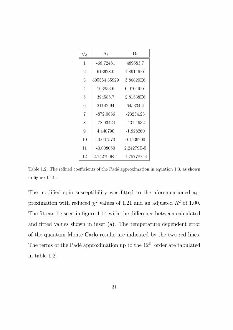
1.2 The refined coefficients of the Pade approximation in equa-
tion 1.3, as shown in figure 1.14, . . . . . . . . . . . . . . 31
3.1 Atomic positional parameters of CuCrO4 (space group
Cmcm ) as obtained from a profile refinement of the x-ray
powder diffraction pattern collected at room temperature.
The lattice parameters amount to a = 5.43877(50) A,
b = 8.97225(83) A and c = 5.89044(55) A. . . . . . . . . 53
xxiv

3.2 The spin exchange parameters of CuCrO4 as found by
GGA+U calculations with the two different on-site repul-
sions Ueff = 4 and 6 eV. The left column for each Ueff
contains the direct theoretical results, while the values in
the right column are the scaled theoretical results such
that Jnnn equals the experimental finding of -27 K. The
rightmost column summarizes the experimentally found
spin exchange values. The final row shows the Curie-
Weiss temperatures of the scaled GGA+U spin exchange
parameters, calculated using the mean field expression;
θCW = 13
∑i
ziJiS(S+1), where zi is the number of neigh-
bours with which a single atom interacts via the spin ex-
change Ji, and the experimentally found values from elec-
tron paramagnetic resonance and magnetic susceptibility
measurements. . . . . . . . . . . . . . . . . . . . . . . . . 75
4.1 The values for the fits to the molar magnetic susceptibility
displayed in figure 4.5, the errors are given in parentheses.
(v) and (f) denote a varied or fixed quantity, respectively. 93
xxv
4.2 Values of the spin exchange parameters J1 - J3 (in K) for
TiPO4 obtained by mapping the GGA+U total energies
of the four spin configurations, see figure. 4.11, onto the
Hamiltonian details are given in the text. . . . . . . . . . 107
4.3 The predicted atomic parameters for TiPO4, in the space
group Pmmn. . . . . . . . . . . . . . . . . . . . . . . . . 108
xxvi

Introduction
The study of solid materials, their properties and their phases is known
as condensed matter physics. It is a very wide, varied, research field,
ranging from the study of single atoms on a substrate to the phase
transitions of bulk samples and beyond.
A subsection of these studies focusses on magnetic phenomena. Mag-
netism is a integral part of condensed matter physics and consists of
many sub-fields. Initially the only known (ferro) magnetic materials
were the three ferrous transition metals, iron, cobalt and nickel and a
few naturally occurring, more complex, minerals. Later new compounds
were synthesized/discovered that had new and interesting characteris-
tics.
Magnetic materials are normally discussed as either itinerant or non-
itinerant. Itinerant magnets are systems where the magnetic moments
are non-localized. This is generally realized in metals where there is a
spin polarization of the electrons at the Fermi surface. Non-itinerant
magnets, which are the subject of this PhD thesis, have a well defined
magnetic moment and are typically insulating materials. Here I concen-
trate on 3d transition metal oxides where the interplay of spin, charge
and orbital degrees of freedom can result in a plethora of magnetic prop-
xxvii

erties.
For 3d ions with open shells magnetism and hence the magnetic mo-
ment can be rather well understood within the Russel-Saunders coupling
scheme. Here S is the spin, an intrinsic property of a particle (1/2 for
an electron), and L is the angular momentum. Both are good quan-
tum numbers. For f electrons, namely the 4f Lanthanoids and to some
extent also the 5f Actinoids series, the magnetic properties are best de-
scribed by the quantum number J which is the total angular momentum.
The total angular momentum of the ground-state is, for the less than
half full occupation of the f -levels, the absolute value of the difference
between L and S , |L - S |, and the sum of L and S for the more than
half full situation, i.e. |L + S | . However, for the transition metals, the
3d, 4d and 5d series, the magnetic properties can often be well described
by using spin only because of the quenching of the orbital angular mo-
mentum. This PhD thesis will only concern itself with the magnetism of
3d transition metals, hence only the quantum number S is of relevance.
The work that follows concentrates on non-itinerant transition metal
compounds that exhibit characteristics of one-dimensional magnetism.
The first chapter will concentrate on characteristics of one-dimensional
magnetism, some phenomena of one-dimensional magnets and some known
compounds. The second chapter will describe the experimental and com-
xxviii
putational methodology used for the investigations reported here. The
third and fourth chapters focus on the presentation of two new magneti-
cally one-dimensional systems, CuCrO4 and TiPO4. Despite both being
essentially isostructural and S = 1/2 systems they exhibit very different
magnetic properties.
xxix

Chapter 1
Magnetism
In this chapter I will discuss some elementary concepts of magnetism and
then focus in more detail on low dimensional magnetism. In particular
aspects of multiferroicity and other systems, that are pertinent to my
PhD work, will be reviewed.
1.1 Magnetism
Magnetism is a wide and vivid research area. This thesis will concentrate
on a small subsection of the vast field of physics, namely on 3d non-
itinerant, one-dimensional magnetism. Here 3d refers to the electrons
that contribute to the magnetism of transition metals. Non-itinerant
means that the magnetic moment is confined to an atom or atoms. This
1

is the case for non-conducting materials. More information can be found
in many condensed matter text books [1, 2, 3].
1.1.1 The magnetic moment
For many transition metals the magnetic moment is best described by the
spin quantum number S. Scaling linearly with the g-factor the effective
magnetic moment, which enters into the Curie law is given as
µeff = g√
S(S + 1).
The magnetic susceptibility χ(T) of a set of free uncoupled spin entities
is given by the Curie-law:
χ(T) =C
T
with
C =NAµ
2eff
3kB.
In the case of exchange interaction between the magnetic centers the
magnetic susceptibility is given by the Curie-Weiss law
χ(T) =C
T − θ.
Provided that the thermal energy kBT is significantly larger than the
exchange interaction energy. The Curie-Weiss temperature θ is given by
θ =1
3
∑i
ziJiSi(Si + 1)
2

where zi is the number of neighbours with which a single atom interacts
via the spin exchange Ji.
It the temperature becomes comparable with the typical spin exchange
interaction energy one generally encounters magnetic ordering phenom-
ena. These depend on many details of the lattice arrangement, crystal
anisotropies. Magnetic ordering phenomena on highly anisotropic lat-
tices, i.e. lattices in which spin exchange interactions along a special
direction are predominant, are the subject of this thesis. Generally, one
encounters regimes of extended short-range correlations before at suffi-
ciently low-temperatures long-range magnetic ordering appears.
The electronic g-factor is 2, but values slightly greater or smaller than 2
are seen for real systems since spin-orbital coupling perturbs the system
in such a way that;
geff = g − f(λ . . .)
here f(λ . . .) scales linearly with λ, the spin-orbital coupling constant.
The absolute value of λ generally increases as one progresses through
the transition metal series, with the exception of S = 5/2 (Mn2+ or
Fe3+) where it is effectively zero. The sign of the spin-orbital coupling
also changes as on progresses through the transition metal series. For
transition metals with less than half filled shells, e.g. Ti3+, λ is positive,
but for the more than half filled shells, when one is dealing with quasi-
3

particles (holes), λ is negative. As such one expects a g-factor of slightly
less than 2 for Ti3+ and more than 2 for Cu2+.
1.1.2 Crystal electric field
For a free 3d transition metal atom one finds a surrounding spherical
electron cloud with all 5 3d states degenerate in energy. But when that
atom is put into a material the 3d electron clouds distort and the energy
levels are no longer degenerate. This is the effect of the crystal electric
field of the other surrounding ions. It originates from an electrostatic
interaction. When a transition metal is in an oxygen octahedral envi-
ronment the 5 3d states are split into a doublet, eg, higher in energy and
a triplet t2g that is lower in energy, the former can be filled by 4 and
the latter by 6 electrons. An elongation or compression of the octahedra
results in a further splitting of the energy levels. The 3d orbitals and
the orbital energy landscape are shown in figure 1.1.
4

(a)
(b)
(c)
Figure 1.1: Taken from magnetism and magnetic materials by J. M. D. Coey [1].(a):
The five orbitals of the 3d transition metals. (b): The energy splitting of the 3d orbitals
(from left to right); a free atom, an atom in a triangular based pyramid environment, an
atom in a non-distorted octahedral environment and an atom in a cubic environment.
(c): The energy landscape of the 3d orbitals in an elongated (left) and a compressed
(right) octahedral environment.
The Pauli exclusion principle states that electrons with the same quan-
tum numbers can not occupy the same space. Hence, each orbital can
5

accommodate two electrons one with spin up and one with spin down.
The electrons fill the orbitals starting with the lowest one in energy.
It is not always energetically advantageous (due to Coulomb repulsion)
for two electrons to occupy the same orbital. In some cases the elec-
trons half fill the lowest energy orbitals and then continue to half fill the
higher energy orbitals. This is known as the high-spin configuration and
it is common for some magnetic atoms e.g. Fe3+ and Mn2+. When the
electrons totally fill the lower energy orbitals first the arrangement is
known as the low-spin configuration. This is shown in figure 1.2. More
information can be found in most magnetism text books [4].
Figure 1.2: A pictorial representation of the high- and low-spin configurations for Fe3+.
1.1.3 Interactions
Exchange interactions are integral to long-range magnetic ordering. They
can take many forms: Ruderman-Kittel-Kasuya-Yosida (RKKY) inter-
6
action, direct exchange, double exchange and superexchange to name a
few. Here I will introduce the three forms of exchange that are pivotal
to non-itinerant magnetism and this PhD work.
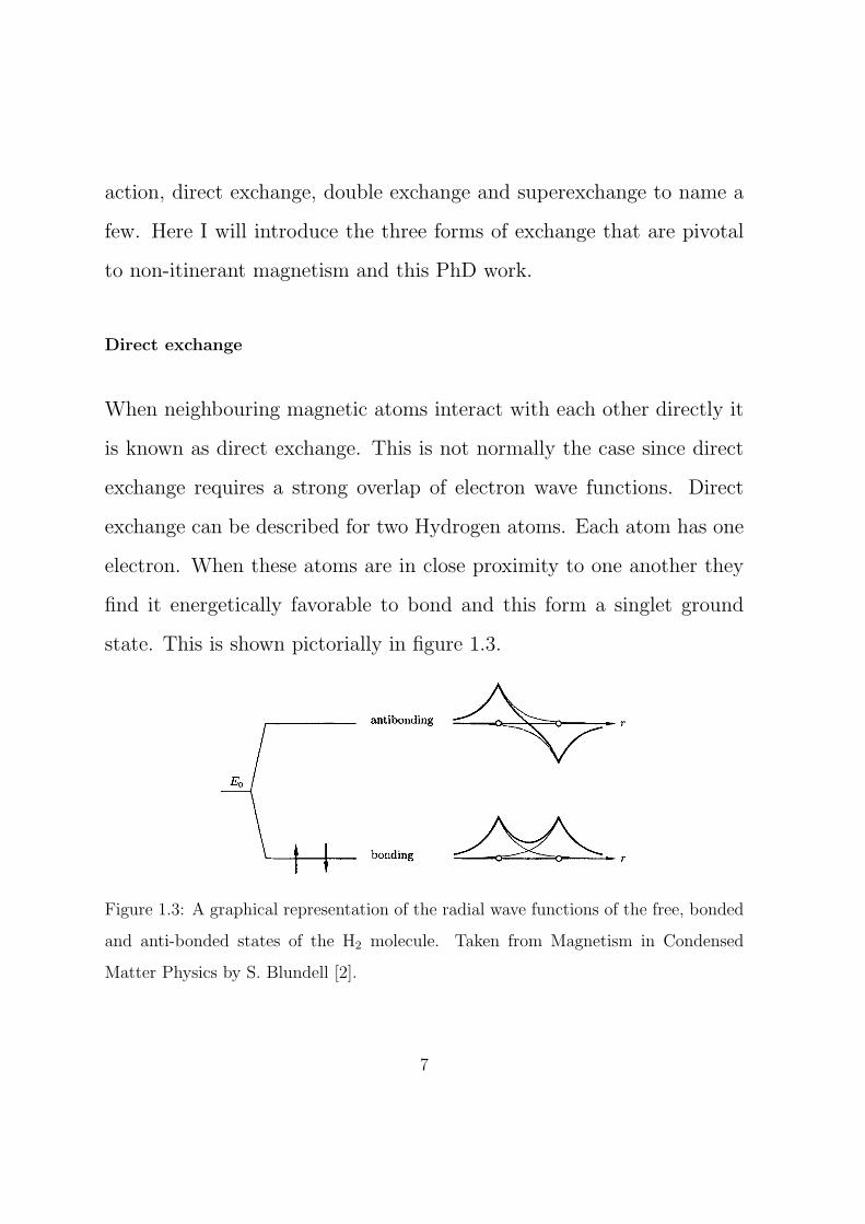
Direct exchange
When neighbouring magnetic atoms interact with each other directly it
is known as direct exchange. This is not normally the case since direct
exchange requires a strong overlap of electron wave functions. Direct
exchange can be described for two Hydrogen atoms. Each atom has one
electron. When these atoms are in close proximity to one another they
find it energetically favorable to bond and this form a singlet ground
state. This is shown pictorially in figure 1.3.
Figure 1.3: A graphical representation of the radial wave functions of the free, bonded
and anti-bonded states of the H2 molecule. Taken from Magnetism in Condensed
Matter Physics by S. Blundell [2].
7

Mediated exchange
Mediated exchange, sometimes also known as superexchange, indirect
exchange or Kramers-Anderson superexchange, is exchange between two
magnetic atoms mediated through a diamagnetic only atom such as O2−
or F−. It acts over a longer distance than direct exchange and it is
integral to most non-itinerant magnets. It arises from the hybridization
of the transition metal’s d electrons and the mediator’s p electrons. A
p electron hops from the O2− or F− to the transition metal in the same
manner as for the direct exchange mechanism. A d electron from the
other transition metal atom the hops into the empty p hole. This creates
an excited state, which relaxes when the p electrons return to the O2−
or F− orbitals. The sign of the exchange is governed by the orbitals
involved and their arrangement with regards to one another. This can
be seen as two direct exchange pathways. The exchange pathways can
become very large, sometimes including an additional direct O2− · · ·O2−
or F− · · ·F− exchange.
Anisotropic exchange terms
The interaction between two spins can generally be given by
H = S i · J i,j · S j,
8

where J i,j is a 3×3 tensor that contains all information pertaining to the
spin exchange interaction. The tensor can take the decomposed form,
J i,j = T i,j + Ai,j.
Here T i,j is the symmetric component of J i,j and Ai,j is the antisym-
metric component. This is an important relativistic spin exchange inter-
action is known as the Dzyaloshinski-Moriya (DM) interaction. It takes
the form of an extra term in the exchange Hamiltonian given by
HDM = −1
2
∑ij
Dij · S i × S j,
here the DM interaction is represented by the DM vector, Dij. A non-
zero DM vector generally requires a low-symmetry environment with
the absence of an inversion center. DM interactions are reported to play
a major role in one-dimensional chain compounds and other transition
metal oxides and could possibly give rise to multiferroicity [5, 6].
1.1.4 Spin models
In a simple interpretation, spin models can be classed by the dimension-
ality of the spin. The simplest one-dimensional spin model is known as
the Ising model. This is where an infinite easy axis anisotropy confines
the magnetic moments to ± z direction. The two-dimensional model,
called the XY model, occurs when an easy plane anisotropy confines the
9
magnetic moments to the xy -plane. In this case there is no z -axis com-
ponent of the magnetic moment entering into the exchange Hamiltonian.
The final, three-dimension model, the Heisenberg model, is isotropic and
has components of the magnetic moment in all three cartesian coordi-
nates.
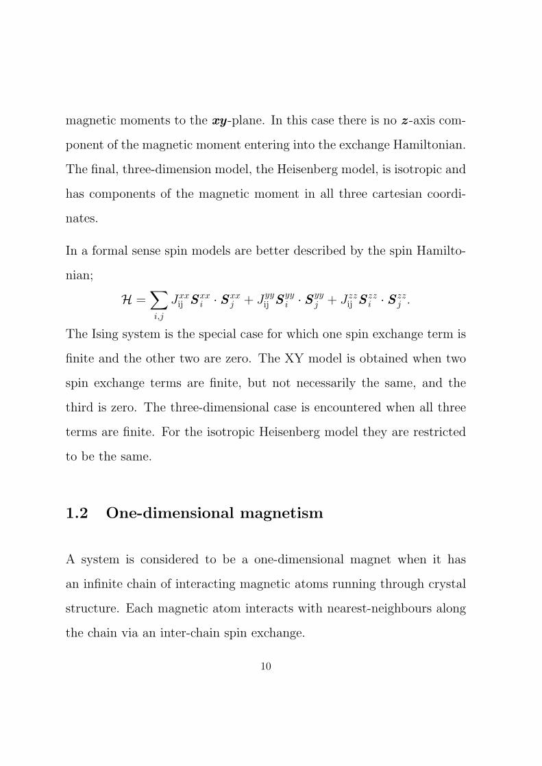
In a formal sense spin models are better described by the spin Hamilto-
nian;
H =∑i,j
Jxxij Sxx
i · Sxxj + Jyy
ij Syyi · S yy
j + Jzzij S
zzi · S zz
j .
The Ising system is the special case for which one spin exchange term is
finite and the other two are zero. The XY model is obtained when two
spin exchange terms are finite, but not necessarily the same, and the
third is zero. The three-dimensional case is encountered when all three
terms are finite. For the isotropic Heisenberg model they are restricted
to be the same.
1.2 One-dimensional magnetism
A system is considered to be a one-dimensional magnet when it has
an infinite chain of interacting magnetic atoms running through crystal
structure. Each magnetic atom interacts with nearest-neighbours along
the chain via an inter-chain spin exchange.
10

It is a common occurrence that within the chain the nearest-neighbour
(nn) atoms generally interact strongly. However, the next nearest-neighb-
our (nnn) atoms can, in some cases (that will be discussed later), also
interact via a strong, if not stronger, spin exchange interaction. The nn,
nnn spin exchange interactions are indicated pictorially in figure 1.4.
nn
nnn
Figure 1.4: A simplified one-dimensional chain of atoms, with the nn and nnn spin
exchange interactions indicated.
In the situation of nn, nnn anti-ferromagnetic spin exchange interactions
the system becomes frustrated and not all spin exchange interactions can
be satisfied simultaneously. This is demonstrated in figure 1.5. Frustra-
tion can also result from nn ferromagnetic and nnn anti-ferromagnetic
spin exchange interactions.
11

AFM
AFM
?
Figure 1.5: A pictorial representation of a frustration in one-dimensional lattice.
One-dimensional magnetism shows itself in many different ways, some
of which will be discussed below. A characteristic is a broad hump in
the magnetic susceptibility as shown for a uniform nn non-alternating
Heisenberg spin chain in figure 1.6. The hump is due to short-range
magnetic correlation. It has been rigorously proven by Mermin-Wagner
that for truly one-dimensional systems and two-dimensional Heisenberg
magnets there is no long-range ordering at finite temperature [7]. This is
why there is no sudden drop in the magnetic susceptibility in figure 1.6.
For real systems there is generally a drop or kink in the magnetic sus-
ceptibility due to long-range magnetic ordering. This will be discussed
later.
12

Figure 1.6: The magnetic susceptibility of a uniform nn Heisenberg spin chain with
Jnn = 1 and a g-factor = 2, calculated using the Pade approximation put forth by
Johnston et al. [8].
1.2.1 Multiferroicity
A multiferroic is a material that exhibits more than one form of order,
e.g. anti-/ferromagnetic, anti-/ferroelectric and or anti-/ferroelastic or-
dering [9]. Multiferroics can be split into two groups, type-I and type-II.
Type-I, or proper multiferroics, are systems which have two or more in-
dependent ’ferroic’ subsystems. These materials have two or more order
parameters that are not coupled with one another and appear at dif-
13

ferent temperatures. Well known examples include BiMnO3 or PbVO3
[10, 11]. More pertinent to this work are type-II multiferroics, tradi-
tionally referred to as improper multiferroics. Within these systems,
ferroelectricity does not exist independently of magnetic order [12, 13].
For spin 1/2 systems ferroelectricity can be the result of a helicoidal spin
density wave, for which inversion symmetry is broken upon entering the
long-range ordered states [5]. At the phase transition, long-range order-
ing, the sample goes from paramagnetic and dielectric to a magnetically
ordered ferroelectric. It has been formulated by Katsura, Nagaosa and
Balatsky and Mostovoy [14, 5] that for such a case a relationship ex-
ists between the electrical polarization P , the vector e12 connecting the
two spins S1 and S1 and the cross product of the magnetic moments of
neighbouring spins [S1×S2], as given by;
P ∝ e12 × [S1 × S2].
1.2.2 Some known low-dimensional S = 1/2 quantum spin
chains
Helicoidal magnetic ordering can be realized in one-dimensional systems
which have competing nn and nnn spin exchange interactions. Figure
1.7 demonstrates the phase diagram of nn, nnn spin exchange inter-
actions on a one-dimensional lattice. The phase diagram is split into
14
three sections. An anti-ferromagnetic phase exists between Jnnn = 0
with Jnn anti-ferromagnetic and approximate values corresponding to
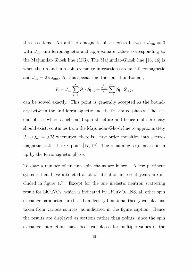
the Majumdar-Ghosh line (MG). The Majumdar-Ghosh line [15, 16] is
when the nn and nnn spin exchange interactions are anti-ferromagnetic
and Jnn = 2×Jnnn. At this special line the spin Hamiltonian;
E = Jnn
∞∑i=1
Si · Si+1 +Jnn2
∞∑i=1
Si · Si+2,
can be solved exactly. This point is generally accepted as the bound-
ary between the anti-ferromagnetic and the frustrated phases. The sec-
ond phase, where a helicoidal spin structure and hence multiferroicity
should exist, continues from the Majumdar-Ghosh line to approximately
Jnnn/Jnn = 0.25 whereupon there is a first order transition into a ferro-
magnetic state, the FF point [17, 18]. The remaining segment is taken
up by the ferromagnetic phase.
To date a number of nn nnn spin chains are known. A few pertinent
systems that have attracted a lot of attention in recent years are in-
cluded in figure 1.7. Except for the one inelastic neutron scattering
result for LiCuVO4, which is indicated by LiCuVO4 INS, all other spin
exchange parameters are based on density functional theory calculations
taken from various sources, as indicated in the figure caption. Hence
the results are displayed as sections rather than points, since the spin
exchange interactions have been calculated for multiple values of the
15

on-site repulsion, U .
Figure 1.7: The nn nnn spin exchange phase diagram for S = 1/2 one-dimensional
system, adapted from Bursill et al. [17]. The coloured sections/lines are density func-
tional theory calculations for real systems, except the line labeled LiCuVO4 INS which
is based on an inelastic neutron scattering results [19, 20, 21, 22, 23, 24].
Some examples of multiferroic systems are described in more detail be-
low.
16

LiCuVO4
LiCuVO4 is a well known intrinsically low-dimensional type-II multifer-
roic [19, 23, 25, 26]. At ≈ 2.4 K LiCuVO4 undergoes long-range order-
ing and becomes multiferroic. It has been reported to have a helicoidal
spin spiral structure with ferromagnetic nn and anti-ferromagnetic nnn
spin exchange interaction [25]. The multiferroicity is evidenced by an
anomaly in the dielectric properties and a spontaneous electrical polar-
ization, as shown in figure 1.8.
Figure 1.8: Main (o): The relative dielectric constant of LiCuVO4 versus temperature.
Inset (o): The electrical polarization of LiCuVO4, calculated from the pyroelectric
current, versus temperature. Taken from Schrettle et al. [26].
17
CuCl2
CuCl2 was the subject of many investigations which probed its multifer-
roic behaviour at low-temperature [20, 27]. CuCl2 undergoes long-range
ordering at 23.9(1) K as evidenced by specific heat, magnetic suscep-
tibility and elastic neutron scattering experiments, see figure 1.9 and
the citation(s) therein. At long-range ordering a sharp spike is seen
in the dielectric constant below which there is a spontaneous electrical
polarization. At lower temperatures, immediately below the long-range
ordering anomaly, the relative dielectric constant starts to grow. With
decreasing temperature it levels off and then starts to decrease. This
has the appearance of a broad asymmetric hump. With the application
of a magnetic field the spike does not change but the hump decreases
in size and moves to higher temperatures. The dielectric constant and
spontaneous polarization are displayed in figure 1.10.
18
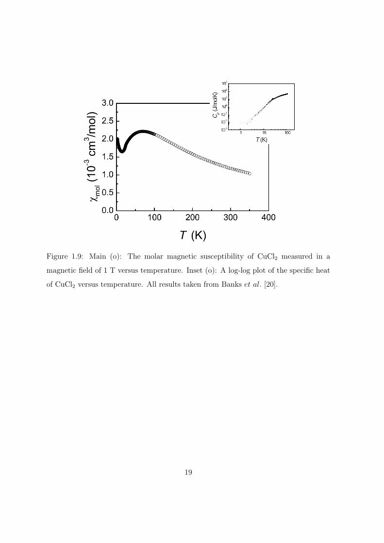
Figure 1.9: Main (o): The molar magnetic susceptibility of CuCl2 measured in a
magnetic field of 1 T versus temperature. Inset (o): A log-log plot of the specific heat
of CuCl2 versus temperature. All results taken from Banks et al. [20].
19
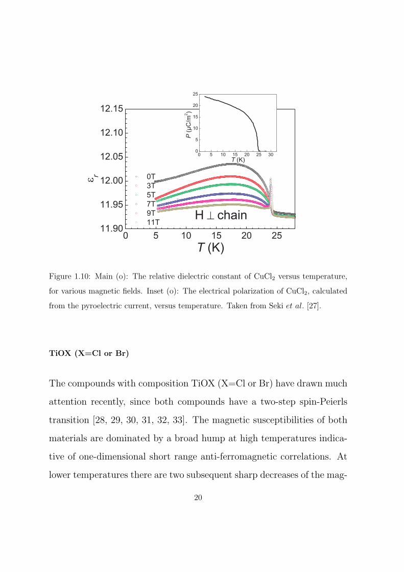
Figure 1.10: Main (o): The relative dielectric constant of CuCl2 versus temperature,
for various magnetic fields. Inset (o): The electrical polarization of CuCl2, calculated
from the pyroelectric current, versus temperature. Taken from Seki et al. [27].
TiOX (X=Cl or Br)
The compounds with composition TiOX (X=Cl or Br) have drawn much
attention recently, since both compounds have a two-step spin-Peierls
transition [28, 29, 30, 31, 32, 33]. The magnetic susceptibilities of both
materials are dominated by a broad hump at high temperatures indica-
tive of one-dimensional short range anti-ferromagnetic correlations. At
lower temperatures there are two subsequent sharp decreases of the mag-
20

netic susceptibility, leaving only a finite van Vleck plus diamagnetic con-
tribution and a small paramagnetic impurity. The spin-Peierls transition
in both compounds happens in two steps: The first transition (drop in
magnetic susceptibility at 92 and 47 K for the Cl and Br compounds,
respectively) is a second order or continuous transition from a param-
agnetic phase into a structurally incommensurate phase. At the second
transition at 67 and 28 K for Cl and Br, respectively, a drop in magnetic
susceptibility is observed. At lowest temperature both samples become
fully dimerised. This transition is first order and hysteretic in nature. A
new crystal structure has been reported for TiOCl below 28 K [34]. For
more information see the cited articles.
1.2.3 Inter-chain couplings and long-range ordering
Generally, weak inter-chain spin exchange interactions, J⊥, lead to long-
range magnetic ordering at sufficiently low-temperatures. One can es-
timate the inter-chain coupling from the long-range ordering tempera-
ture. Yasuda et al. calculated the Neel temperature (TN) of a quasi
one-dimension Heisenberg anti-ferromagnet on a cubic lattice with the
isotropic inter-chain coupling J⊥, inducing three-dimensional long-range
magnetic ordering at TN [35]. By scaling their quantum Monte Carlo
simulations they extrapolate for infinite system size, a relationship be-
21

tween inter- and intra-chain coupling, given by;
TN/|J⊥| = 0.932
√ln(A) +
1
2ln(ln(A)), (1.1)
where A= 2.6 J∥/TN and J∥ is the intrachain spin exchange constant.
1.2.4 Electron paramagnetic resonance theory
Oshikawa and Affleck [36, 37] developed a theory for the electron para-
magnetic resonance of S = 1/2 quasi-one-dimensional chain compounds
at low-temperatures which have anisotropic or antisymmetric exchange
terms i.e. Jxx = Jyy = Jzz. At low-temperatures near long-range
ordering they found that there is a positive linear slope of the line-
width with increasing temperature. The proportionality constant de-
pends upon many aspects and as such no quantitative results can be
obtained easily. But there is a system independent factor of 2 between
the proportionality pre-factors parallel and perpendicular to the easy
axis. Such as;
δw⊥easy axis
δw∥easy axis= 2,
where,
δw =∂(HWHM)
∂T.
22
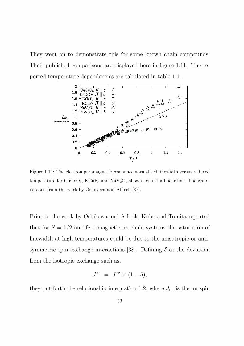
They went on to demonstrate this for some known chain compounds.
Their published comparisons are displayed here in figure 1.11. The re-
ported temperature dependencies are tabulated in table 1.1.
Figure 1.11: The electron paramagnetic resonance normalised linewidth versus reduced
temperature for CuGeO3, KCuF3 and NaV2O5 shown against a linear line. The graph
is taken from the work by Oshikawa and Affleck [37].
Prior to the work by Oshikawa and Affleck, Kubo and Tomita reported
that for S = 1/2 anti-ferromagnetic nn chain systems the saturation of
linewidth at high-temperatures could be due to the anisotropic or anti-
symmetric spin exchange interactions [38]. Defining δ as the deviation
from the isotropic exchange such as,
Jzz = Jxx × (1− δ),
they put forth the relationship in equation 1.2, where Jnn is the nn spin
23

δw (T/K) Compound Orientation
4.2×10⁻⁴ CuGeO3 B∥c
4.7×10⁻⁴ CuGeO3 B∥a
17×10−4 KCuF3 B∥c
22×10−4 KCuF3 B∥a
1.3×10⁻⁴ NaV2O5 B∥c
0.65×10⁻⁴ NaV2O5 B∥b
Table 1.1: The half width at half maximum for known low-dimensional chain com-
pounds as shown in figure 1.11, taken from the work by Oshikawa and Affleck [37].
exchange, and ∆H is half line-width at half maximum of the electron
paramagnetic resonance absorption line.
∆H(T → ∞) ≈ δ2
gµBJnn(1.2)
Now that I have given an introduction to one-dimensional magnetism I
will discuss as a first result a Pade approximation for the temperature
dependence magnetic susceptibility of a S = 32 Heisenberg quantum anti-
ferromagnetic spin chain.
24

1.2.5 Pade approximation for the molar magnetic susceptibil-
ity of a S = 32 Heisenberg quantum anti-ferromagnetic
spin chain
One-dimensional magnetic systems can be characterized by magnetic
susceptibility, see section 1.2. Being able to model the temperature
dependent magnetic susceptibility of a one-dimensional system is very
helpful since values such as the nn spin exchange interaction and the
g-factor can be ascertained.
A Pade approximation is a useful tool in mathematics to approximate a
given function. Pade approximations have been widely used in modern
condensed matter physics for fitting observables, e.g. the molar magnetic
susceptibility or specific heat. A well known and highly cited example
is the Pade approximation for the molar magnetic susceptibility and the
specific heat of a S = 1/2 Heisenberg alternating chain, as put forth by
D. C. Johnston et al. [8]. Within the paper Johnston et al. discussed a
non-alternating S = 1/2 Heisenberg chain. In the spirit of Johnston’s
work, the Pade approximation for the magnetic susceptibility of a S = 32
Heisenberg quantum anti-ferromagnetic spin chain was formulated from
results obtained by quantum Monte Carlo simulations for a S = 3/2
Heisenberg chain.
25
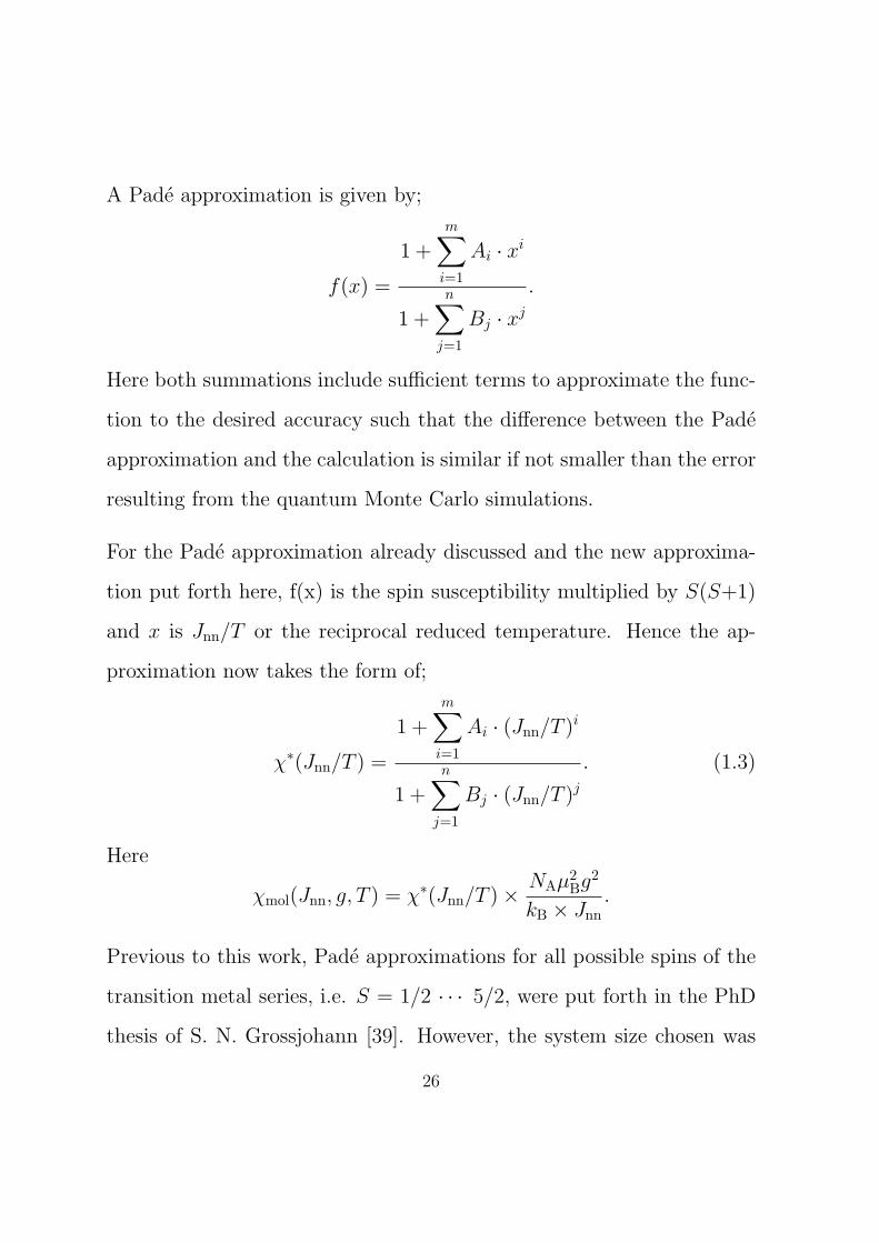
A Pade approximation is given by;
f(x) =
1 +m∑i=1
Ai · xi
1 +n∑
j=1
Bj · xj.
Here both summations include sufficient terms to approximate the func-
tion to the desired accuracy such that the difference between the Pade
approximation and the calculation is similar if not smaller than the error
resulting from the quantum Monte Carlo simulations.
For the Pade approximation already discussed and the new approxima-
tion put forth here, f(x) is the spin susceptibility multiplied by S(S+1)
and x is Jnn/T or the reciprocal reduced temperature. Hence the ap-
proximation now takes the form of;
χ∗(Jnn/T ) =
1 +m∑i=1
Ai · (Jnn/T )i
1 +n∑
j=1
Bj · (Jnn/T )j. (1.3)
Here
χmol(Jnn, g, T ) = χ∗(Jnn/T )×NAµ
2Bg
2
kB × Jnn.
Previous to this work, Pade approximations for all possible spins of the
transition metal series, i.e. S = 1/2 · · · 5/2, were put forth in the PhD
thesis of S. N. Grossjohann [39]. However, the system size chosen was
26

rather small, 512 spins and as such the results severely suffered from
finite size effects at relatively high temperatures. Previous to the work
by Grossjohann a trivial approximation was put forth by Hiller et al. [40].
Previous to all of these works, Fischer put forth a classical approximation
for any spin system [41]. A comparison of the three previous works
pertaining to the temperature dependent magnetic susceptibility of a
S = 3/2 spin chain and our quantum Monte Carlo calculations are shown
in figure 1.12. The previous non-classical work suffers from finite size
effects and the quantum Monte Carlo results being reported here are
more accurate and closer to the true temperature dependent magnetic
susceptibility of such a chain. A S = 3/2 system is best described as
being a quantum spin system and as such the classical approach does
not describe the system adequately.
27
0 10 200.5
1.0
1.5
2.0 QMC 2000 spins Grossjohann SSE 512 spins Classical approximation Hiller et al. approximation
S
(S+1
)(101 )
kBT/JNN
Figure 1.12: (o): Our quantum Monte Carlo results, see text for more information.
Solid blue line: The Pade approximation by Grossjohann [39]. Solid green line: The
classical approximation put forth by Fischer [41]. Solid black line: The approximation
by Hiller et al [40].
The modified spin susceptibility for a S = 3/2 anti-ferromagnetic Heisen-
berg spin chain was calculated using the looper algorithm on a cluster
within the ALPS suite. For more details see section 2.6.1. Initially the
magnetic susceptibility was calculated at sufficiently low values of T/Jnn
for different system sizes, so as to ascertain a system size that would
be acceptable to reproduce what would be observed for a real system
(N ≫ NA), the results are shown in figure 1.14 insets b. A system size
28

Figure 1.13: Left: The scaled computation time versus system size at a reduced tem-
perature of 0.05. Right: The arbitrary computation time versus spin, at a reduced
temperature of 0.05.
of N = 2000 was chosen, since for systems sizes N ≥ 2000 converging
values of the spin susceptibility were obtained within error bars, see fig-
ure 1.14 (b). Bigger systems could have been chosen but this would
have drastically increased computation times for little gain. The scaling
of computation time with both system size and spin can be seen in fig-
ure 1.13. A clear non-linear scaling can be seen for both variables, the
system size scaling is exponential as one would expect.
29

0 10 200.5
1.0
1.5
2.0
101
kBT/JNN
0 10 20-2
-1
0
1
2
(b)
calc-
padé
10
4
kBT/J
NN
(a)
0 1000 2000 30006.0
6.2
6.4
6.6
calc
102
N
kBT/JNN=0.05
Figure 1.14: Main: (o): The temperature dependent modified spin susceptibility for a
S = 3/2 spin chain with nn spin exchange interactions, calculated by quantum Monte
Carlo using the ALPS suite, versus reduced temperature. Solid red line: A fit to a Pade
approximation as discussed in the text. (a): (o): The difference between the modified
spin susceptibility as calculated by quantum Monte Carlo and the Pade approximation
fitted to the simulation. The solid red lines denotes the boundaries of the error bars
given for the quantum Monte Carlo calculation. (b) The modified spin susceptibility for
different systems sizes at a fixed reduced temperature of 0.05. N denotes the number
of spins.
30
i/j Ai Bj
1 -68.72481 489583.7
2 613928.0 1.89146E6
3 805554.35929 3.86820E6
4 703853.6 6.07049E6
5 394585.7 2.81538E6
6 21142.94 645334.4
7 -872.0836 -23234.23
8 -78.03424 -431.4632
9 4.440790 -1.928260
10 -0.067570 0.1536200
11 -0.008050 2.24279E-5
12 2.742790E-4 -1.75778E-4
Table 1.2: The refined coefficients of the Pade approximation in equation 1.3, as shown
in figure 1.14, .
The modified spin susceptibility was fitted to the aforementioned ap-
proximation with reduced χ2 values of 1.21 and an adjusted R2 of 1.00.
The fit can be seen in figure 1.14 with the difference between calculated
and fitted values shown in inset (a). The temperature dependent error
of the quantum Monte Carlo results are indicated by the two red lines.
The terms of the Pade approximation up to the 12th order are tabulated
in table 1.2.
31

1.3 Summary
In this chapter I discussed multiferroicity and low-dimensional mag-
netism with an emphasis on what is relevant for this PhD thesis. I
also discussed relevant materials that will be commentated on in the
following chapters.
The next chapter will give a brief overview of experimental methodology
and computation that will be used to characterize CuCrO4 and TiPO4
in the latter chapters.
32

Chapter 2
Experimental methodology and
computation
In this chapter I will discuss and explain the experimental methodology
and computations that were used to characterize the systems reported
on in the following chapters. This chapter is meant to be a concise
experimental overview. More information can be found in the pertinent
manuals and the published papers.
33

2.1 X-ray and neutron diffraction
2.1.1 Single crystal diffraction
CAD4 diffractometer
CAD4 is a four circle diffractometer manufactured by Enraf Nonius, that
allows data acquisition from 0 ≤ θ ≤ 2π and 0 ≤ ϕ ≤ π. It employs non-
monochromated Ag radiation (0.5608 A). The machine was primarily
used for orientating single crystals.
STOE IPDS diffractometer
The STOE IPDS diffractometer is a two circle diffractometer. It uses an
imaging plate detector which allows data acquisition from 0 ≤ θ ≤ 2π.
It uses non-monochromated Ag radiation (0.5608 A). The machine was
primarily employed for crystal structure determination.
2.1.2 Powder diffraction
Lab-based x-ray diffractometers
Two x-ray powder diffractometers were used, both STOE Stadi P ma-
chines. One machine produced monochromated Cu x-ray radiation (Cu-
34
Kα1 1.54056 A) and the other used monochromated Mo x-ray radi-
ation (Mo-Kα1 0.70930 A). Both are equipped with Germanium(111)
monochromators, and as such both select fully monochromated Kα1 ra-
diation. The advantage of having access to MoKα1 is such that it allows
one to measure elements that would absorb the frequently used Cu radia-
tion, e.g. Cr. The samples were mounted in thin walled quartz capillaries
(∅ = 0.3 or 0.1mm). This technique allows for preparation in a glove
box and hence patterns of air sensitive samples could be easily collected
[42].
High resolution powder diffractometer for thermal neutrons - HRPT
HRPT is a high resolution thermal neutron powder diffractometer. It
was designed for small samples and has a resolution comparable to those
of synchrotron x-ray powder diffraction studies, with a possible resolu-
tion of ≤ 0.05◦. The machine is located at SINQ in the Paul Scherrer
Institute, Switzerland. A schematic can be seen in figure 2.1.
35

Figure 2.1: Schematic of the powder diffractometer HRPT at the Paul Scherrer Insti-
tute (Switzerland) [43].
2.2 Magnetisation
2.2.1 SQUID magnetometry
Magnetisation was measured using a Quantum Design Magnetic Prop-
erty Measurement System, or MPMS for short. The machine allows the
measurement of magnetisation in the range of ± 7 T in the temperature
range 1.85 K to 400 K. An additional oven insert enables measurements
36

in the higher temperature range of 300 K to 800 K. The sample, whether
it is a powder or crystal, was generally mounted in the sample holder by
two different methods. The simplest and fasted method has the sample
contained within a diamagnetic only gelatine capsule, which weighs ap-
proximately 40 mg. The raw magnetisation could then be later corrected
for the magnetisation of the sample holder. A gelatine capsule is shown
in figure 2.2. The second, more time consuming method, was mounting
the sample in a suprasil c⃝ quartz tube. The tube is thin walled, so as
to add the smallest background signal possible. It is sealed half way
up its length, in a manner that deforms the longitudinal distribution
of weight as little as possible, i.e. the longitudinal mass distribution
(mg/cm) remains relatively constant. This could never be fully guaran-
teed, but measurements of the magnetisation of such a sealing yielded a
magnetic susceptibility of ≈ 10−9 emu/Oe for which the raw data could
be corrected. Once the sample was mounted, the tube was evacuated
and flushed with helium gas a few times. This ensured that there was
no O2 gas that would give an additional signal at low-temperature and
provide a good thermal contact to the cryostat. The tube was finally
sealed. A sealed tube and the seal half way up the tube are displayed in
figure 2.3.
37

Figure 2.2: Left: A filled gelatine capsule as used for measuring the magnetization.
Right: A disassembled, empty, gelatine capsule, prior to use for measuring magnetiza-
tion.
Figure 2.3: Left: A filled and sealed quartz tube ready for magnetization measurements.
Right: A closer view of the seal half way up the tube.
38
The molar magnetic susceptibility could be calculated from the raw mag-
netisation by
χmol[cm3/mol] =
M(T,H)[emu]×m[g]
Mm[g/mol]× H[Oe]
where M(T,H)[emu] is the measured magnetisation, m[g] is the mass of
the sample, Mm[g/mol] is the molar mass of the sample and H[Oe] is the
applied magnetic field.
The magnetic susceptibility also required correcting for the diamagnetic
contribution resulting from the closed shells of the atoms contained
within the sample. The values are well known and tabulated by Sel-
wood [44]. An example which is relevant to this work would be Cu2+
which has a diamagnetic contribution of -11 × 10−6 cm3/mol.
In addition to the diamagnetic signal of the samples, an additional pos-
itive temperature independent van Vleck contribution also needed to be
subtracted from the magnetic susceptibility. The van Vleck contribu-
tion, sometimes referred to as the van Vleck temperature independent
paramagnetism, arises from the population of the magnetic states that
are higher in energy than the magnetic ground state. As such, it is sys-
tem specific quantity. For Cu2+ it typically amounts to values between
20 × 10−6 cm3/mol and 120 × 10−6 cm3/mol depending on the direction
39

of the applied magnetic field with respect to the crystal axes.
2.3 Specific heat
2.3.1 Relaxation calorimetry
Specific heat was measured using a Quantum Design Physical Property
Measurement System (PPMS), via the relaxation technique. The ma-
chine allows the measurement of multiple physical properties, but for this
work only the specific heat option was used. The specific heat was mea-
sured in the magnetic field range of ± 9 T and in the temperature range
of 1.85 K to 350 K. An additional 3He insert allows one to measure down
to ≈ 400 mK. Crystals were mounted to a thermally decoupled sample
holder by Apiezon c⃝ vacuum grease. A pre-measurement, an ”addenda”
measurement, was done before mounting the sample so that the specific
heats of the sample holder and the Apiezon c⃝ vacuum grease could be
subtracted from the total specific heat, yielding the specific heat of the
sample.
Powders could also be measured on a PPMS sample holder, either by
pelletizing and mounting it in the same way as crystals or by slightly
melting the Apiezon c⃝ grease, once the addenda has been measured, and
adding the powder. The slightly molten Apiezon c⃝ vacuum grease would
40

allow the powder to sink into it and thermally anchor the sample. A
typical sample investigated by this method weighed approximately 2 mg.
2.3.2 Adiabatic Nernst calorimeter
A home built quasi-adiabatic Nernst-type calorimeter was also used. It
allowed one to measure specific heat in the temperature range 2.0 K to
300 K. The machine’s construction and testing has been the subject of M.
Banks’ PhD thesis [45]. The calorimeter can accommodate single crystal
and powder samples. The powder samples were first housed in a flat
bottom high purity glass bell jar filled with helium gas. The mass of the
glass must be known so it can be subtracted later from the total specific
heat. An empty and full glass bell jars are shown in figure 2.4. This is
discussed in depth in M. Banks’ thesis. The sample, be it a powder or
a single crystal, is then attached to a thermally isolated sapphire plate,
which has a heater and a calibrated thermometer, via Apiezon c⃝ vacuum
grease. See the aforementioned thesis for more details.
41

Figure 2.4: Top: An empty glass bell jar. Bottom: A full sealed glass bell jar, ready
for specific heat measurements; left is a view from the top and right is a view from the
side.
2.4 Electron Paramagnetic Resonance spectroscopy
The electron paramagnetic resonance spectra were collected on a home
built microwave spectrometer. The spectrometer operates at ∼ 9.5 GHz
(X-band). The required field was created by an iron core Bruker BE25
magnet equipped with a BH15 field controller. The cryostat is a contin-
uous flow system and can operate in the range of 3 K to 295 K. There
are two sample mounts. The first is an electron paramagnetic resonance
neutral low-background suprasil c⃝ quartz tube. The second is an elec-
42
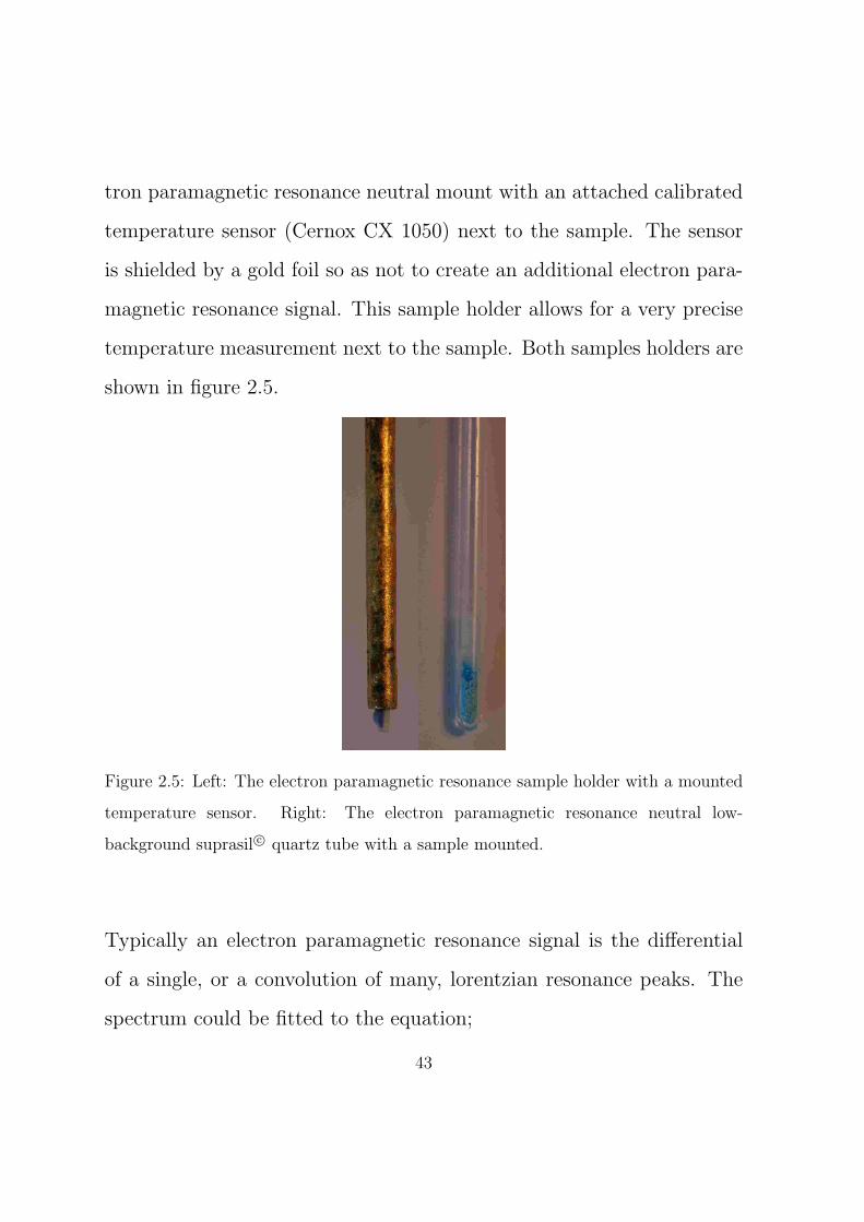
tron paramagnetic resonance neutral mount with an attached calibrated
temperature sensor (Cernox CX 1050) next to the sample. The sensor
is shielded by a gold foil so as not to create an additional electron para-
magnetic resonance signal. This sample holder allows for a very precise
temperature measurement next to the sample. Both samples holders are
shown in figure 2.5.
Figure 2.5: Left: The electron paramagnetic resonance sample holder with a mounted
temperature sensor. Right: The electron paramagnetic resonance neutral low-
background suprasil c⃝ quartz tube with a sample mounted.
Typically an electron paramagnetic resonance signal is the differential
of a single, or a convolution of many, lorentzian resonance peaks. The
spectrum could be fitted to the equation;
43

EPRsignal =N∑i=1
d(Li(H))
dH+ y0 + y1 × H+ y2 × H2, (2.1)
where y0, y1 and y2 are variable background terms, N represents the
total number of peaks and L(H) is given as;
L(H) =I
π× ∆w+ α× (H− Hres)
(H− Hres)2 + (∆w)2. (2.2)
Where I is the intensity, ∆w is the half width at half maximum, Hres
is the resonance position and α is the dispersion. When an electron
paramagnetic resonance signal is very broad, the negative field resonance
should also be included.
The g-factor can be ascertained from the resonance field Hres by
gµBHres = hν. (2.3)
Hence,
g =0.71449× ν[MHz]
Hres[G],
where ν is the applied microwave frequency.
44

2.5 Dielectric capacitance
Dielectric capacitances were measured with either an Andeen-Hagerling
AH2500A or an AH2700 capacitance bridge. Both are high precision
variable AC-voltage bridges. The latter has a variable frequency option,
50 to 20000 Hz in discrete steps, whereas the former operates at a fixed
1000 Hz frequency. Samples were mounted via two methods. The first
method, used for single crystals or pelletized powders, involved creating
contacts on either side, with silver paint/paste or by depositing gold
on the surface. Gold wires where then connected to the contacts which
in turn where soldered to co-axial copper wire that led to the bridge.
The second method applicable for powder samples only, had the powder
compacted and sandwiched between two copper pistons in a vespelr
tube. The copper pins were then in turn connected to co-axial copper
wire which led to the bridge. All measurements where done in an Oxford
helium cryostat equipped with a variable temperature insert allowing
temperatures between 1.2 K and 300 K using a 12 T superconducting
magnet.
45
2.6 Computation
2.6.1 Algorithms and Libraries for Physics Simulations - ALPS
”The ALPS project (Algorithms and Libraries for Physics Simulations)
is an open source effort aiming at providing high-end simulation codes
for strongly correlated quantum mechanical systems as well as C++
libraries for simplifying the development of such code. ALPS strives to
increase software reuse in the physics community.” [46]
The ALPS v1.3.5 project incorporates many programs. The two most
pertinent programmes to this work are the looper code for quantum
Monte Carlo simulations [47] and the Full Diagonalization Package for
exact solutions of finite systems. The looper code allows the calcula-
tion of observables such as spin magnetisation, spin susceptibility, spe-
cific heat and staggered magnetisation for large (N ≥ 1000) finite sys-
tems. For such large systems the observables can be assumed to be
those of an infinite system, with only very low-temperature observables
(T/J < 0.01) showing a deviation from an infinite system, i.e. an N de-
pendence for large N (N ≥ 1000). This makes quantum Monte Carlo a
very powerful tool for simulating different systems. However, the quan-
tum Monte Carlo approach has a problem. When it comes to frustrated
systems it encounters the sign problem [48] and the solution does not
46

converge. This is where the second package, Full Diagonalization, comes
into play. Full Diagonalization allows one to exactly solve the hamil-
tonian for a finite system and as such calculate observables. But the
system size is heavily limited by computing power and more importantly
by RAM memory capacity. As such modern computers can only solve
S = 1/2 systems for approximately 24 atoms. With larger spins the
system size has to be significantly reduced. This results in deviations
(finite size effects) at relatively large temperatures, T/J < 0.3. How-
ever, with these limitations in mind Full Diagonalization can be used to
obtain observed behaviour in many systems.
2.7 Summary
In this chapter I briefly described the experimental method used for
characterization of the systems discussed in the other chapters.
In the next chapter I will be discussing our investigation of CuCrO4.
This is a chemically well-known compound but its magnetic properties
have never been studied until now. We reported in our publication, that
CuCrO4 is a previously unknown type-II multiferroic [24].
47

Chapter 3
CuCrO4 - A new multiferroic
material
In this chapter I will discuss the magnetic properties of CuCrO4, a
S = 1/2 3d9 spin chain. Here I am reporting a detailed experimen-
tal and theoretical investigation characterizing the magnetic properties
of CuCrO4 for the first time.
48
3.1 Crystal structure
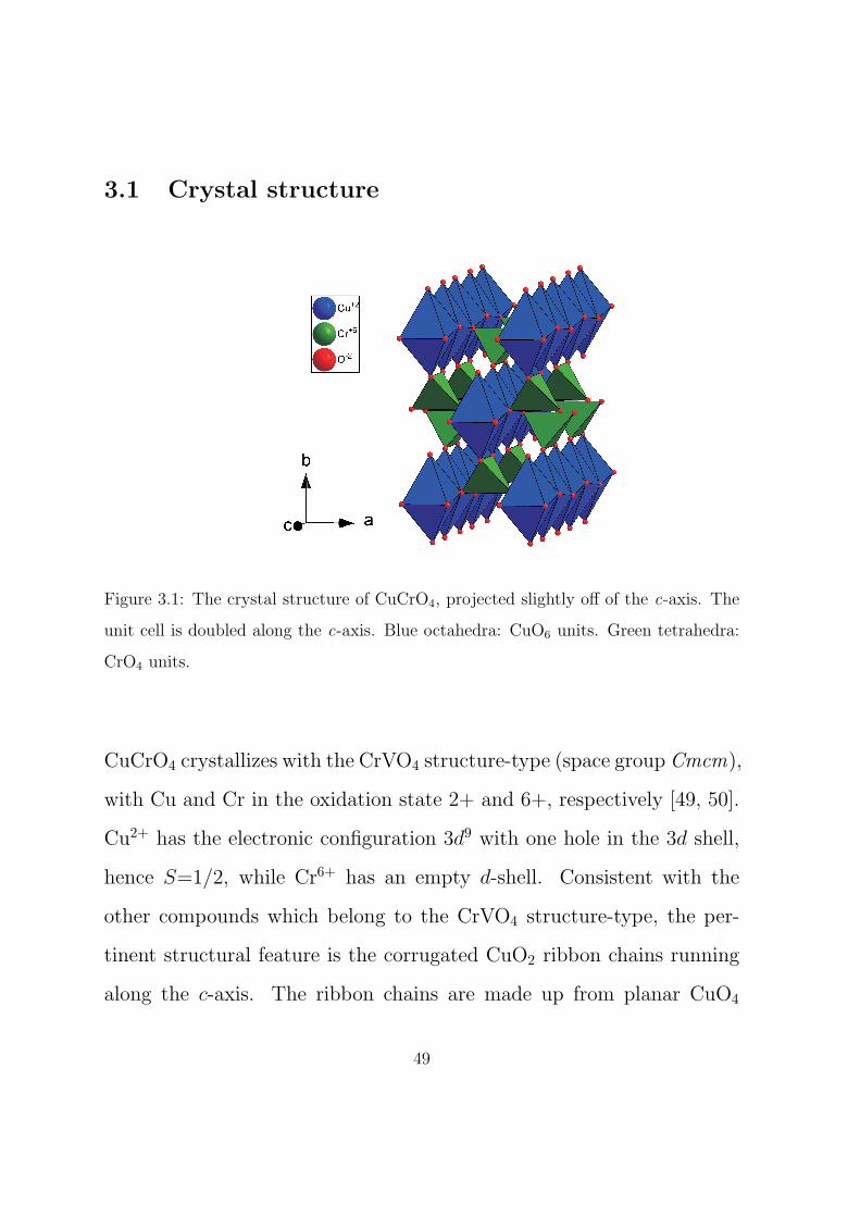
Figure 3.1: The crystal structure of CuCrO4, projected slightly off of the c-axis. The
unit cell is doubled along the c-axis. Blue octahedra: CuO6 units. Green tetrahedra:
CrO4 units.
CuCrO4 crystallizes with the CrVO4 structure-type (space group Cmcm),
with Cu and Cr in the oxidation state 2+ and 6+, respectively [49, 50].
Cu2+ has the electronic configuration 3d9 with one hole in the 3d shell,
hence S=1/2, while Cr6+ has an empty d-shell. Consistent with the
other compounds which belong to the CrVO4 structure-type, the per-
tinent structural feature is the corrugated CuO2 ribbon chains running
along the c-axis. The ribbon chains are made up from planar CuO4
49

plaquettes which are connected via trans-edges, as shown in figure 3.1.
The CuO4 plaquettes form the basis of elongated (Jahn-Teller distorted)
CuO6 octahedra. The ribbon chains are interconnected by slightly dis-
torted CrO4 tetrahedra, which inhabit interstitial voids. At room tem-
perature the Cu2+· · ·Cu2+ distance is reported to be 2.945(2) A with a
Cu2+· · ·O2−· · ·Cu2+ angle of 97.067(7)o [50].
3.2 Sample preparation
The preparation of CuCrO4 is rather intriguing, mainly due to the insta-
bility of the copper-chromate 1:1:4 stoichiometry. According to Hanic
et al. at rather low-temperatures CuCrO4 decomposes into the spinel-
type CuCr2O4 and CuO [51]:
4CuCrO4687 K − 773 K−−−−−−−−−→ 2CuO + 2CuCr2O4 + 3O2.
So-far this seriously hampered the growth of crystals, suitable for bulk
characterization, as well as the preparation of highly homogenous sam-
ples.
The second problem associated with sample preparation is a health and
safety concern, Cr6+ is considered a genotoxic carcinogen [52]. As such
all samples must be handled with care.
50

Multiple methods can be employed to prepare polycrystalline sample of
CuCrO4. All measurements reported here were undertaken on a single
powder sample (≈ 160 mg total available sample) that was prepared
by separately dissolving equimolar amounts Copper(II) hydroxide and
Chromium(VI) oxide in distilled water∗. The two solutions were mixed
and boiled to dryness. The resulting powder was heat treated in air at
a temperature of 150◦C for 2 days. This method was first described by
Arsene et al. [53]. The phase purity of the sample was checked by x-ray
powder diffraction measurements using a STOE STADI-P diffractome-
ter with monochromated Mo-Kα1 radiation. The powder pattern was
fitted using the Rietveld profile refinement method employed within the
Fullprof Suite [54]. No other reflections besides those of CuCrO4 were
observed. The pattern and the resultant fit can be seen in figure 3.2. The
structural parameters of this fit are tabulated in table 3.1. Later, larger
samples intended for powder neutron diffraction were prepared along a
similar route replacing Copper(II) hydroxide by anhydrous Copper(II)
acetate. It should be noted that the sample is reported and was found
to be brick red in colour. But black samples, initially believed to be
decomposed samples, can also be obtained. According to x-ray powder
diffraction are isostructural to their red counterparts. The only differ-
ence in their preparation was a longer or higher annealing temperature.
∗The sample was prepared by Prof. R. Glaum and his group at Bonn University, Bonn.
51

5 10 15 20 25 30 35
0.0
0.5
1.0
Co
un
ts(a
rb.u
nits)
2q (°)
Figure 3.2: (o): Measured x-ray powder diffraction pattern of CuCrO4 (λ = 0.70930 A
). Solid red line: Calculated pattern (Rp = 13.1%, reduced χ2 = 1.15) using the
parameters given in table 3.1. Solid blue line: The offset difference between measured
and calculated patterns. The positions of the Bragg reflections used to calculate the
pattern are marked by the green vertical bars in the lower part of the figure.
3.3 Magnetic susceptibility
The molar magnetic susceptibility of a powder sample of CuCrO4, con-
tained within a gelatin capsule was measured in the temperature range
of 2 K to 350 K in an applied dc magnetic field of 1, 3, 5 and 7 T. Above
≈ 20 K no field dependence was observed, suggesting minimal ferromag-
netic impurities. However, upon cooling a noticeable field dependence
became apparent. At lowest temperatures an almost asymptotic be-
52

oxidation Wyckoff position
atom state and letter x y z Biso
Cu +2 4a 0.0000(0) 0.0000(0) 0.0000(0) 0.089(8)
Cr +6 4c 0.0000(0) 0.3700(3) 0.2500(0) 0.904(7)
O1 -2 8f 0.0000(0) 0.2652(5) 0.0312(9) 0.800(12)
O2 -2 8g 0.2326(7) -0.0198(6) 0.2500(0) 0.800(12)
Table 3.1: Atomic positional parameters of CuCrO4 (space group Cmcm ) as obtained
from a profile refinement of the x-ray powder diffraction pattern collected at room
temperature. The lattice parameters amount to a = 5.43877(50) A, b = 8.97225(83) A
and c = 5.89044(55) A.
haviour was observed for small fields, with a kink at ≈ 8 K and an
ill-defined shoulder ranging from ≈ 11 to 20 K. In small magnetic fields
a thermal hysteretic behaviour was seen below the ill-defined shoulder.
Upon application of a larger magnetic field the molar magnetic suscepti-
bility decreased and the asymptotic and hysteretic behaviour died away.
The kink became more pronounced and it is interpreted as evidence
of long-range magnetic order. The ill-defined shoulder gradually faded
away and was replaced by a well-defined hump, which is indicative of
one-dimensional short range correlations, with a maximum centered at
≈ 15 K.
53
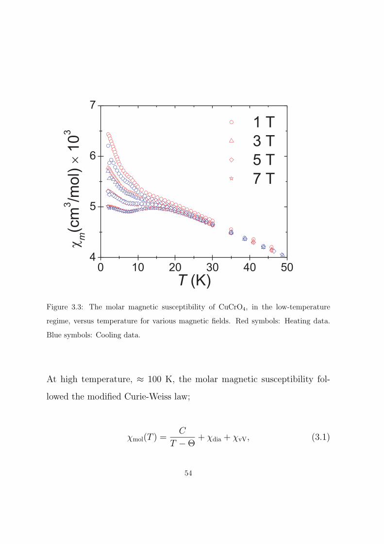
Figure 3.3: The molar magnetic susceptibility of CuCrO4, in the low-temperature
regime, versus temperature for various magnetic fields. Red symbols: Heating data.
Blue symbols: Cooling data.
At high temperature, ≈ 100 K, the molar magnetic susceptibility fol-
lowed the modified Curie-Weiss law;
χmol(T ) =C
T −Θ+ χdia + χvV, (3.1)
54

where C is the Curie constant pertaining to the spin susceptibility of the
Cu2+ entities. The Curie constant is given as C = NAg2 µ2
B S(S + 1)/3kB.
χdia refers to the diamagnetic susceptibilities of the electrons in the closed
shells which could be estimated from the tabulated increments given by
Selwood as -62×10−6 cm3/mol [44]. The χvV contribution can not be
tabulated and can not be calculated precisely, but values are known for
similar compounds and comparisons can be made (see above).
55

0 100 200 3000
250
500
750
1000
1/c
m(m
ol/cm
3)
T (K)
Figure 3.4: (o): The inverse molar magnetic susceptibility versus temperature of
CuCrO4, measured in a field of 7 T. Red solid line: Fit to the modified Curie-Weiss
law as given in equation 3.1.
Best agreement was found with a g-factor of 2.17(2), a Θ of -56(1) K and
χdia + χvV ≈ +20 × 10−6 cm3/mol. This implies a χvV of ≈ +80 × 10−6
cm3/mol which is a reasonable value for Cu2+ in this environment [20].
56
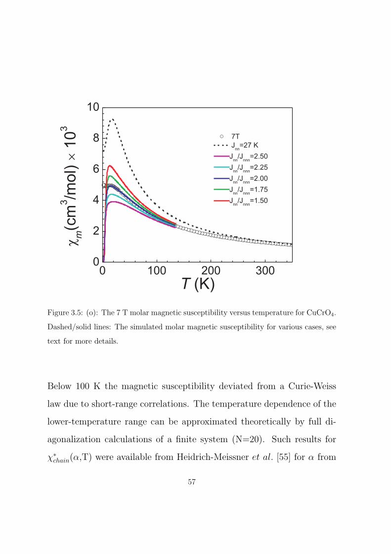
Figure 3.5: (o): The 7 T molar magnetic susceptibility versus temperature for CuCrO4.
Dashed/solid lines: The simulated molar magnetic susceptibility for various cases, see
text for more details.
Below 100 K the magnetic susceptibility deviated from a Curie-Weiss
law due to short-range correlations. The temperature dependence of the
lower-temperature range can be approximated theoretically by full di-
agonalization calculations of a finite system (N=20). Such results for
χ∗chain(α,T) were available from Heidrich-Meissner et al. [55] for α from
57

+4 to -4, where α=Jnn/Jnnn. Guided by density functional theory cal-
culations (see sections 3.7) values of α ranging from 1.5 to 2.5 were
compared to the experimental data along with the molar magnetic sus-
ceptibility of a uniform nn anti-ferromagnetic chain [8]. Inter-chain spin
exchange interactions could be approximated with a mean-field correc-
tion, such as
χmol(T ) =χchain(T )
1− λ× χchain(T )+ χ0,
where λ is given by
λ =1
NAg2µ2B
∑i
ziJiSi(Si + 1).
Here Ji is an inter-chain spin exchange interaction constant that occurrs
zi times for a given atom with spin Si. χ0 can be taken from above,
≈ +20 × 10−6 cm3/mol. A g-factor of 2.125 was used, which is con-
sistent with electron paramagnetic resonance measurements, see section
3.5. Jnnn was scaled so as to reproduce the hump at the correct temper-
ature. The results are shown in figure 3.5. It is apparent from the graph
that best agreement is obtained for an α ≈ 2, Jnnn = -27 K and a λ of
7(1) mol/cm3. z1 = 4, z2 = 2 was assumed for the density functional the-
ory calculations. As shown by the density functional theory calculations
58
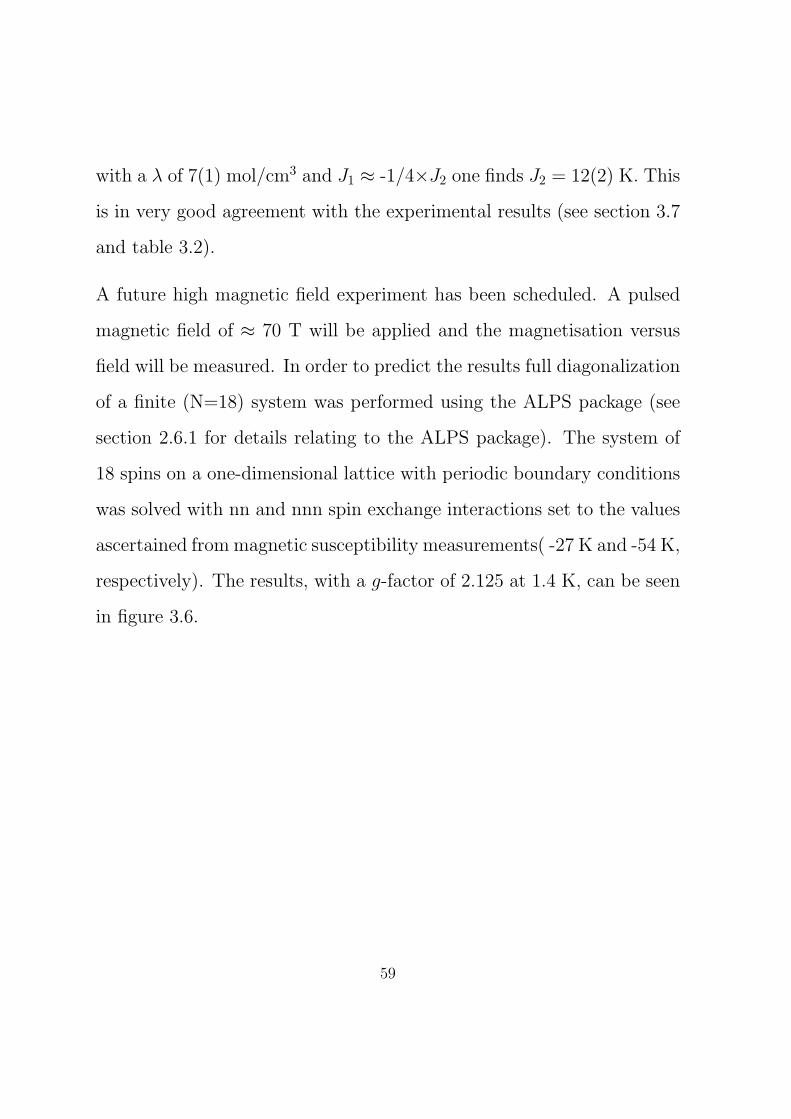
with a λ of 7(1) mol/cm3 and J1 ≈ -1/4×J2 one finds J2 = 12(2) K. This
is in very good agreement with the experimental results (see section 3.7
and table 3.2).
A future high magnetic field experiment has been scheduled. A pulsed
magnetic field of ≈ 70 T will be applied and the magnetisation versus
field will be measured. In order to predict the results full diagonalization
of a finite (N=18) system was performed using the ALPS package (see
section 2.6.1 for details relating to the ALPS package). The system of
18 spins on a one-dimensional lattice with periodic boundary conditions
was solved with nn and nnn spin exchange interactions set to the values
ascertained from magnetic susceptibility measurements( -27 K and -54 K,
respectively). The results, with a g-factor of 2.125 at 1.4 K, can be seen
in figure 3.6.
59

Figure 3.6: Full diagonalization results. Solid red and black lines are the magnetisation
and d(M)d(H)
versus applied magnetic field, respectively.
3.4 Specific heat
The specific heat versus temperature of CuCrO4 was measured on a
powder sample of 2.43 mg (see figure 3.7 and for experimental details
see section 2.3). A broad, smeared, λ-type anomaly centered at 8.2(2) K
can be clearly seen. This is indicative of long-range magnetic ordering.
60

Within figure 3.7 there is also presented the specific heat measured with
an applied magnetic field of 9 T. The data is offset so as to be clearly
distinguishable from the 0 T data. Within error bars the data for the two
different fields are identical. This implies that the long-range ordering
anomaly does not shift as a function of applied magnetic field. The intra-
chain is ≈ -27 K, this is substantially larger in energy than 9 T and as
such one would not expect a significant change of the spin arrangement.
Specific heat divided by temperature is plotted versus temperature and
it is shown in figure 3.8. This plot allows an estimation to be made
of the entropy contained within the long-range ordering anomaly. ∆S
≈ 0.6 J/mol.K was found to be contained within the anomaly. This is
≈ 10 % of the expected total magnetic entropy for a S = 1/2 system,
S = R ln(2S+1). For S = 1/2 we obtain R ln(2), where R is the molar
gas constant. The other 90% of the entropy has been removed by short-
range correlations at higher temperatures. At long-range ordering the
single ribbon chains are high correlated and most of the entropy left
pertains to the ordering of the chains with respect to each other.
61
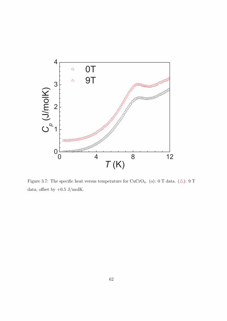
0 4 8 120
1
2
3
4
0T
9T
Cp
(J/m
olK
)
T (K)
Figure 3.7: The specific heat versus temperature for CuCrO4. (o): 0 T data. (△): 9 T
data, offset by +0.5 J/molK.
62

Figure 3.8: (o): The specific heat divided by temperature versus temperature for
CuCrO4, in the temperature range of the anomaly.
The low-temperature specific heat, below the long-range ordering tem-
perature, consists of both phonon and magnon contributions. The tem-
perature dependence of the phonon contribution could be assumed to fol-
low a Debye ∝ T 3 power law, whereas the magnon contribution varies in
a manner depending upon the spin wave dispersion relation. For three-
dimensionally ordered samples one expects, for anti-ferromagnetically
63

long-range ordered materials, a contribution to the specific heat with
a temperature dependence similarly to that of the phonon contribution
∝ T 3. When the sample is ferromagnetic magnons provide a ∝ T 3/2
contribution [56]. Figure 3.9 displays a plot of Cp/T3/2 versus T 3/2.
Since the data shows a non-zero intercept one can infer that the spe-
cific heat comprises of a ∝ T 3/2 contribution indicative of a contribution
of ferromagnetic magnons. This is consistent with the density func-
tional theory calculations. The linear behaviour in figure 3.9 could be
explained by equation 3.2. β is related to the 0 K Debye tempera-
ture, θD(T →0), by equation 3.3. In the case of CuCrO4 where N =
6 one finds θ(T →0) = 138(1) K. Within ferromagnetic spin-wave the-
ory the non-zero intercept, is given by equation 3.4 [57]. Here Jinter is
the nn inter-chain coupling and q is a constant pertaining to the num-
ber of nearest-neighbours. If we assume a simple cubic arrangement
of nearest-neighbours situation, which is not unreasonable for CuCrO4,
then q = 0.113. With an intercept of 0.0109(1) J/molK5/2 we find Jinter
to be ≈ 19.5 K. Consistent with what was found from ab initio calcula-
tions, see section 3.7.
Cp/T3/2 = βT 3/2 + γ (3.2)
64
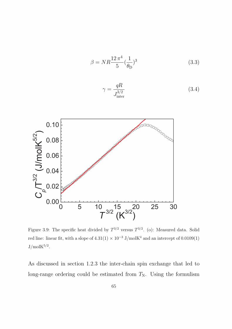
β = NR12 π4
5(1
θD)3 (3.3)
γ =qR
J3/2inter
(3.4)
Figure 3.9: The specific heat divided by T 3/2 versus T 3/2. (o): Measured data. Solid
red line: linear fit, with a slope of 4.31(1) × 10−3 J/molK4 and an intercept of 0.0109(1)
J/molK5/2.
As discussed in section 1.2.3 the inter-chain spin exchange that led to
long-range ordering could be estimated from TN. Using the formulism
65

put forth by Yasuda et al. and assuming J∥ to be the Jnn as found from
magnetic susceptibility, |J⊥| was found to be ≈ 5 K. This is of the same
order of magnitude as the value obtained from density functional theory
calculations, as well as the experimentally ascertained value from the
mean field correction term λ. The difference between the inter-chain
coupling calculated from Yasuda’s formalism and the other values may
arise since CuCrO4 has two different inter-chain coupling constants, J1
and J2, and a nnn spin exchange interaction Jnnn, that was not included
in Yasuda’s model. For CuCrO4 these values are significant and need to
be incorporated.
3.5 Electron paramagnetic resonance
The temperature dependent electron paramagnetic resonance was mea-
sured on a ≈ 5 mg sample mounted in an electron paramagnetic reso-
nance neutral low-background suprasil c⃝ quartz tube, see section 2.4.
A single symmetric, broad Lorentzian line was observed centered at
≈ 3.4 kOe with a temperature dependent peak-to-peak linewidth of
0.8 - 1 kOe. The line could be nicely fitted to the derivative of a
single Lorentzian absorption line with a small dispersion contribution
|α| ≤ 0.04. Since the half width at half maximum was so large, of the
66

same order of magnitude as the resonance position, both circular compo-
nents of the exciting linearly polarized microwave field were taken into
account, i.e. the negative magnetic field resonance centered at -Hres,
see section 2.4. The room-temperature spectrum can be seen in figure
3.10. The dispersion term fitted to the electron paramagnetic resonance
signal was negligible over the whole temperature range and as such was
ignored.
0.1 0.2 0.3 0.4 0.5 0.6-10.0
-7.5
-5.0
-2.5
0.0
EP
Rsig
na
l(a
rb.u
nits)
mBH (T)
297(1) K
Figure 3.10: (o): Electron paramagnetic resonance signal for CuCrO4 taken at
297(1) K. Solid red line: Fit to equation 2.1.
67
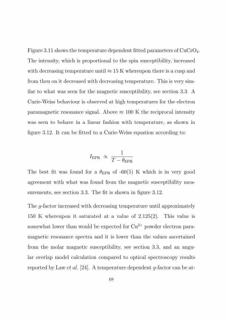
Figure 3.11 shows the temperature dependent fitted parameters of CuCrO4.
The intensity, which is proportional to the spin susceptibility, increased
with decreasing temperature until ≈ 15 K whereupon there is a cusp and
from then on it decreased with decreasing temperature. This is very sim-
ilar to what was seen for the magnetic susceptibility, see section 3.3. A
Curie-Weiss behaviour is observed at high temperatures for the electron
paramagnetic resonance signal. Above ≈ 100 K the reciprocal intensity
was seen to behave in a linear fashion with temperature, as shown in
figure 3.12. It can be fitted to a Curie-Weiss equation according to:
IEPR ∝ 1
T − θEPR
The best fit was found for a θEPR of -60(5) K which is in very good
agreement with what was found from the magnetic susceptibility mea-
surements, see section 3.3. The fit is shown in figure 3.12.
The g-factor increased with decreasing temperature until approximately
150 K whereupon it saturated at a value of 2.125(2). This value is
somewhat lower than would be expected for Cu2+ powder electron para-
magnetic resonance spectra and it is lower than the values ascertained
from the molar magnetic susceptibility, see section 3.3, and an angu-
lar overlap model calculation compared to optical spectroscopy results
reported by Law et al. [24]. A temperature dependent g-factor can be at-
68
tributed to slight changes of the ligand environment as the temperature
decreases. The saturation of the g-factor at low-temperatures supports
this, since the rate of change of the ligand environment would decrease
with decreasing temperature.
69
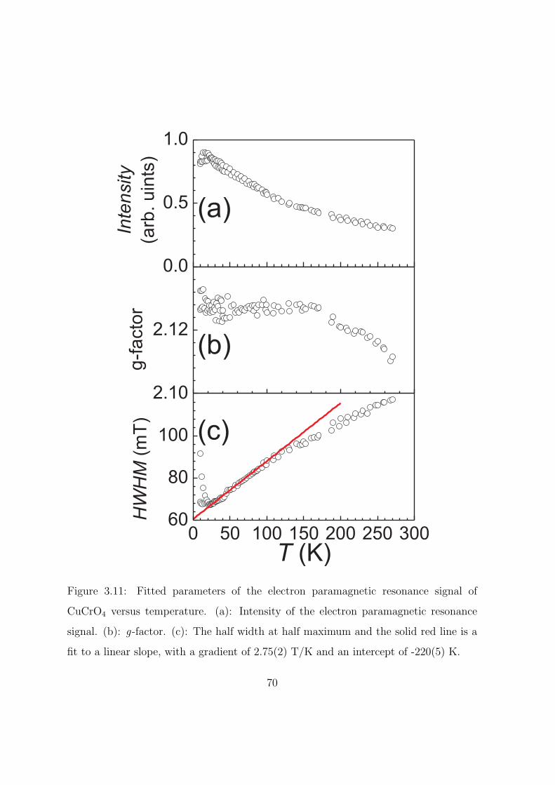
Figure 3.11: Fitted parameters of the electron paramagnetic resonance signal of
CuCrO4 versus temperature. (a): Intensity of the electron paramagnetic resonance
signal. (b): g-factor. (c): The half width at half maximum and the solid red line is a
fit to a linear slope, with a gradient of 2.75(2) T/K and an intercept of -220(5) K.
70

0 100 200 3000.0
0.2
0.4
0.6
0.8
1.0
1/I
nte
nsity
(arb
.u
nits)
T (K)
Figure 3.12: (o): Fitted inverse of the integrated electron paramagnetic resonance
intensity of CuCrO4 versus temperature. Solid red line: Linear fit with an arbitrary
gradient and an intercept of -63.1(1) K.
The half width at half maximum was seen to decrease with decreasing
temperature until ≈ 15 K where it starts to rapidly increase down to
lowest-temperatures. This is indicative of the onset of long-range or-
dering. Within the temperature range of ≈ 25 K to ≈ 100 K the half
width at half maximum increased linearly with increasing temperature,
71

in accordance with results reported by Oshikawa and Affleck (see section
1.2.4). The slope was found to be ≈ 2.5×10⁻⁴ T/K similar to that found
for the spin-Peierls compound CuGeO3 [58]. Deviation away from the
Oshikawa and Affleck behaviour is seen at higher temperatures. The
half width at half maximum then starts to show a concave dependence
with increasing temperature. This is a cross over from the Oshikawa
and Affleck to Kubo and Tomita regime, wherein there is a temperature
independent linewidth. The half width at half maximum is seen to tend
towards a constant temperature independent value, with an extrapolated
saturation value of 0.14 T. Using the formalism put forth by Kubo and
Tomita (see section 1.2.4) this implies a deviation from the symmetric
Heisenberg spin exchange of δ ≈ 3 K or 5% of the nn spin exchange [38].
3.6 ab initio calculations
To understand the magnetic properties of CuCrO4 first principles total
energy calculations were performed†. To examine the magnetic proper-
ties of CuCrO4, the four spin exchange paths shown in figure 3.13 were
considered. Then the spin configuration energies obtained by ab initio
density functional theory calculations were mapped onto a Heisenberg
†The first principle density functional theory calculations were done by Prof. M. Whangbo and
his group at North Carolina State University, Raleigh, N. C., USA.
72

spin exchange Hamiltonian
H = −∑
JijSiSj,
where Jij was the spin exchange for the interaction between spins lo-
cated at lattice sites i and j. The relative energies of the five ordered
spin states of CuCrO4 were determined by density functional calculations
with the Vienna ab initio simulation package, employing the projected
augmented-wave method [59, 60, 61], the generalized gradient approx-
imation (GGA) for the exchange and correlation functional [62], with
the plane-wave cut-off energy set to 400 eV and a set of 64 k-points for
the irreducible Brillouin zone. To account for the electron correlation
associated with the Cu 3d state, GGA plus on-site repulsion (GGA+U)
calculations were performed with Ueff = 4 and 6 eV for Cu [63].
The relative energies of the five ordered spin states obtained from our
GGA+U calculations are summarized in figure 3.13. By mapping these
relative energies onto the corresponding relative energies from the total
spin exchange energies [64, 65, 66, 67, 68], the values of the spin exchange
parameters, Jnn, Jnnn, J1, and J2 could be ascertained as summarized in
table 3.2.
73
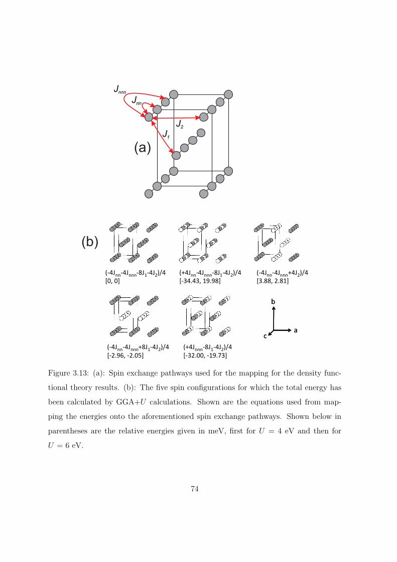
Figure 3.13: (a): Spin exchange pathways used for the mapping for the density func-
tional theory results. (b): The five spin configurations for which the total energy has
been calculated by GGA+U calculations. Shown are the equations used from map-
ping the energies onto the aforementioned spin exchange pathways. Shown below in
parentheses are the relative energies given in meV, first for U = 4 eV and then for
U = 6 eV.
74

Ji Ueff = 4 eV (K) Ueff = 6 eV (K) experiment (K)
Jnn -199.7(1.0) -63.8 -115.9(1.0) -55.4 -54
Jnnn -85.8(0.43) -27 -56.5(0.49) -27 -27
J1 -8.6(0.04) -2.7 -6.00(0.05) -2.9 -4
J2 +31.1(0.16) +9.8 +22.3(0.19) +10.7 +12
θCW -43.2 -38.8 ≈-58
Table 3.2: The spin exchange parameters of CuCrO4 as found by GGA+U calculations
with the two different on-site repulsions Ueff = 4 and 6 eV. The left column for each
Ueff contains the direct theoretical results, while the values in the right column are the
scaled theoretical results such that Jnnn equals the experimental finding of -27 K. The
rightmost column summarizes the experimentally found spin exchange values. The
final row shows the Curie-Weiss temperatures of the scaled GGA+U spin exchange
parameters, calculated using the mean field expression; θCW = 13
∑i
ziJiS(S + 1) [69],
where zi is the number of neighbour with which a single atom interacts via the spin
exchange Ji, and the experimentally found values from electron paramagnetic resonance
and magnetic susceptibility measurements.
Based upon the spin exchange interactions calculated by ab initio meth-
ods, one can predict a magnetic structure. If one assumes the nn spin
exchange interaction to be twice as large as the nnn spin exchange inter-
action and both to be anti-ferromagnetic. Treating only the intra-chain
coupling and assuming the magnetic moment to be a classical vector one
75
can write the energy as
E =∑i
−JSi · Si+1 −∑i
J
2Si · Si+2.
Which can be rewritten as
E = −J |S2|cosθ − J |S2|2
cos2θ,
where θ is the pitch angle between two nn spins. The ground-state is
given as dEdθ = 0. This is the case when θ = ± 60◦, where the nega-
tive and positive results are the two different chiralities (handednesses).
This gives a magnetic unit cell 3 times larger along the c-axis than the
chemical unit cell. The inter-chain spin exchanges would result in a ferro-
magnetic arrangements of chains in the a-axis and an anti-ferromagnetic
arrangement in the b direction. A pictorial representation of this is
shown in figure 3.14. This would imply a magnetic propagation vector
of [0,0,13 ].
76

a
b
(a)
(b)
a
c
Figure 3.14: The predicted magnetic structure of CuCrO4, the chemical unit cell is de-
noted by the dashed box. (a) The magnetic structure in the a-b plane, white and black
circles represent different magnetic moment directions. (b) The magnetic structure
within the a-c-plane, with the magnetic moments represented by an arrow.
3.7 Dielectric capacitance
The dielectric constant, ϵr, versus temperature of CuCrO4 was measured
on a non-pelletized compact powder, see section 2.5, using a AH2700
capacitance bridge with a constant frequency and excitation voltage of
77
1000 Hz and 15 V, respectively. At room-temperature the value ϵr ≈ 48
was observed. Between room-temperature and ≈ 35 K, ϵr was seen to
decrease in a smooth fashion. Between 35 and 15 K ϵr passed through
a shallow double maximum, possibly induced by some magnetostriction
driven by short-range ordering effects above long-range ordering, see
figure 3.15 (b). No reasonable assumptions can be made about the nature
of the shallow double maximum, future neutron scattering experiments
will be needed to probe that is the cause of these features. Just prior to
long-range ordering at 10 K a value of ≈ 4.35 was measured for ϵr.
In zero field, at long-range ordering, ≈ 8.5 K, ϵr started to rapidly in-
crease with decreasing temperature until levelling off and falling once
again, resulting in a rather broad asymmetric hump centered at∼ 5.35 K.
There was no indication for a sharp spike near long-range ordering tran-
sition temperature. This behaviour is frequently found in multiferroic
systems [27, 70]. Similar broad symmetric humps, centered at TN, have
been seen in CuCl2 and CuBr2 [27, 71]. The overall increase of ϵr amounts
to a ≈ 6% effect when compared to the paramagnetic value prior to long-
range ordering. With the application of a magnetic field the maximum
of the magnetoelectric anomaly in ϵr decreases and the maximum of the
broad asymmetric hump moves to higher temperatures. Consistent with
specific heat measurements the onset of the magnetoelectric anomaly,
78

long-range ordering, was not seen to move with an applied field. The
shift of the hump is an artifact from the changing field dependent of ϵr at
different temperatures. The temperature dependence of ϵr under various
magnetic fields is displayed in figure 3.15 within the main panel. The
decrease of ϵr with a magnetic field started above ≈ 1 T and tended to
saturation to the paramagnetic only value at sufficiently high fields. An
isotherm is shown in figure 3.15 (a).
79

Figure 3.15: Main: The temperature dependence of the relative dielectric constant
for CuCrO4 at low-temperatures under various magnetic fields, refer to legend. (a):
A magnetic isotherm of the relative dielectric constant at 5.2(1) K. (b): The relative
dielectric constant of CuCrO4 at higher temperatures in zero magnetic field.
80
3.8 Discussion and conclusion
It was shown in this chapter that at high temperatures CuCrO4 can
be explained as a paramagnet with a Curie-Weiss temperature of ap-
proximately -60 K. This was shown by both magnetic susceptibility
and electron paramagnetic resonance measurements. At lower temper-
atures there are short-range one-dimensional correlations which mani-
fests themselves as a broad hump in the magnetic susceptibility, sim-
ilar to what has been seen for LiCuVO4, CuCl2 and CuBr2 [25, 20,
71]. The electron paramagnetic resonance line width shows a linear
behaviour with temperature at low-temperatures which is indicative of
a one-dimensional magnet with anisotropic or antisymmetric exchange
terms. This has also been seen for LiCuVO4 by Schrettle et al. [70].
The low-temperature magnetic susceptibility was modelled against the
exact diagonalization results for a nn and nnn one-dimensional S = 1/2
spin chain, with a small inter-chain coupling. Agreement was found for
a ratio of Jnn/Jnnn ≈ 2. The position of the broad hump in the magnetic
susceptibility was best replicated with a Jnnn of -27 K.
Long-range ordering was evidenced by a anomaly in the specific heat and
the magnetic susceptibility at ≈ 8.2 K. The dielectric constant exhibits
clear evidence for a magnetoelectric effect at the long-range ordering
81

transition temperature, as seen in other type-II multiferroics. The long-
range ordering anomaly is not seen to move with the application of a
magnetic field. This is indicative of ferromagnetic ordering between the
anti-ferromagnetically ordered chains.
The experimental results were complemented by theoretical ab initio cal-
culations. These confirm a Jnn/Jnnn ratio of approximately 2. However,
density functional theory tends to overestimate spin exchange interac-
tions, typically by a factor of 2-5 [72]. By renormalizing the density
functional theory results to the experimentally observed Jnnn of -27 K,
agrement was found for the inter-chain couplings which were taken from
the correction to the magnetic susceptibility.
However, the renormalized density functional theory results would sug-
gest a Curie-Weiss temperature larger than what has been experimen-
tally observed. This could be due to an insufficient correction of the van
Vleck contribution to the magnetic susceptibility. But the electron para-
magnetic resonance signal is not subject to a van Vleck correction and
as such this argument does not hold for this case. Here the inconsistency
could be due to poor fitting for the electron paramagnetic resonance ab-
sorption line. The counter argument, assuming the experimental results
are correct, could be that there are additional spin exchange interactions
that were not included and have not been taken into account in the mean
82

field approximation of the Curie-Weiss temperature.
On the basis of ab − initio density functional calculations a predictive
magnetic structure could be formulated, which has a spin spiral structure
and a commensurate magnetic propagation vector of [0,0,13 ].
In conclusion, CuCrO4 constitutes a new one-dimensional quantum anti-
ferromagnet, which has a pronounced magnetoelectric anomaly origi-
nating at long-range ordering. Density functional calculations indicate
that CuCrO4 is a one-dimensional anti-ferromagnetic Heisenberg chain
system, where both nn and nnn spin exchange interactions are anti-
ferromagnetic. The ratio Jnn/Jnnn was found to be close to 2, the
Majumdar-Ghosh point [15, 16]. CuCrO4 undergoes long-range ferro-
magnetic ordering due to a sizeable ferromagnetic inter-chain spin ex-
change interaction. The rather large magnetoelectric anomaly below the
Neel temperature provides evidence for non-collinear, possibly helicoidal,
spin ordering in the one-dimensional chains. CuCrO4 is therefore a new
system which exhibits type-II multiferroicity.
3.9 Summary
In the preceding chapter I have shown that CuCrO4 is a quantum spin
chain with type-II multiferroicity. There is still more work to be done
83

on this compound. Especially, elastic and inelastic neutron diffraction
which will given an insight into the magnetic structure. High magnetic
field magnetisation measurements are scheduled to confirm the plateaus
seen in simulations.
A consistent set of spin exchange values has been obtained. Magnetic
and dielectric properties have been measured as a function of temper-
ature and applied magnetic field. Ab initio calculations support the
experimental findings and allow a more informed modelling of the low-
temperature characteristics to be carried out. Further measurements are
needed to support some tentative interpretations of experimental results.
This includes a detailed neutron scattering investigation of the structure
of CuCrO4 at low-temperature.
In the next chapter I will discuss my investigation of the 3d1 system,
TiPO4. TiPO4 is largely isostructural to CuCrO4 and has been the sub-
ject of several, however inconclusive studies of its magnetic properties.
I intend to show that new results which classify TiPO4 as undergoing a
spin-Peierls transition at low-temperature.
84

Chapter 4
TiPO4 - A new spin-Peierls system?
In the following chapter I will report on our investigation into the mag-
netic properties of TiPO4. Unlike the isostructural 3d9 compound CuCrO4,
that was reported on in the previous chapter, TiPO4 undergoes a spin-
Peierls transition and has a non-magnetic ground-state.
4.1 Introduction and crystal structure
TiPO4 is a chemically well known material, but its physical, especially
its magnetic, properties have never been subject to a detailed investiga-
tion. As such no conclusive results have been obtained and no clear
understanding has been gained as of yet. TiPO4 crystallizes in the
CrVO4 structure-type (space group Cmcm) with Ti+3 (3d1 S = 1/2)
85

housed in tetragonally compressed octahedron. The TiO6 octahedra are
edge sharing and arrange themselves in a one-dimensional configuration,
see figure 4.1, forming corrugated ribbon chains running along the c-
axis. The ribbon chains are buckled in the ac-plane with a buckling
angle of 156.927(4)◦. The Ti3+· · ·Ti3+ distance at room-temperature is
3.1745(10) A with a Ti3+· · ·O2−· · ·Ti3+ angle of 95.484(5)◦ [73]. The in-
terstitial voids between the ribbon chains are partially filled by distorted
PO4 tetrahedra.
Figure 4.1: The crystal structure of TiPO4, projected slightly off the c-axis. The unit
cell is doubled along the c-axis. Yellow octahedra: TiO6 units. Purple tetrahedra:
PO4 units.
Previous to this investigation [74] three papers reported the magnetic
86

properties of TiPO4, one by Kinomura et al. [75], a second by Glaum et
al. [76] and a third by Yamauchi and Ueda [77]. The first paper reported
the magnetic susceptibility from 2 K to 600 K and described it as be-
ing “almost temperature independent above 150 K”. The second paper
showed only the reciprocal magnetic susceptibility and simply compares
it to earlier work by Kinomura et al.. However, in this work the authors
also probe the low-temperature (2 K) magnetic structure by neutron
powder diffraction. The authors report no additional reflections due to
coherent magnetic scattering and confirm the low-temperature chemical
structure to remain isostructural to that of the room-temperature struc-
ture, except for a lattice contraction. The authors go on to comment
on their null result, ascribing the absence of magnetic Bragg reflections
as being due to the true one-dimensional linear anti-ferromagnetic na-
ture of TiPO4, wherein no long-range magnetic order would occur at
finite-temperature. The authors of the third paper infer that TiPO4
should have the characteristics of a S = 1/2 Heisenberg antiferromag-
netic chain, quoting ”[A] broad maximum characteristic of a Heisenberg
antiferromagnetic linear chain seems to be above room-temperature”.
The first crystal growth of this compound was reported by Glaum et
al. [78]. They grew single crystals by vapor transport using iodine as a
transport agent.
87

4.2 Sample preparation
Figure 4.2: A single crystal of TiPO4. The orientation and size are indicated.
Single crystals as large as 5×5×2 mm and powder samples of TiPO4 were
prepared via chemical vapor transport∗. An example of a single crystal
can been seen in figure 4.2. The preparation has been the subject of a
previous publication [78], where it was reported that an initial reaction
of
4TiP2O7 + 4TiO2 + TiP −→ 9TiPO4
in an inert atmosphere at 900◦ for 12 hrs, resulted in a pure powder
sample. Going on to chemically vapour transport the powder in an
enclosed quartz ampoule with the temperature gradient 900◦→1000◦
∗The sample was prepared by Prof. R. Glaum and his group at Bonn University, Bonn.
88

(source and sink, respectively), using I2 as a transporting agent (ap-
proximately 200 mg of I2 was used per 15 cm3), resulted in the very high
quality single crystals.
4.3 Magnetic susceptibility
The molar magnetic susceptibility of a collection of many small randomly
oriented crystals, contained within a suprasil c⃝ quartz tube, as discussed
in detail already in section 2.2.1, was measured in the temperature range
of 2 to 400 K in an applied dc magnetic field of 0.1, 1, 3, 5 and 7 T and in
the temperature range from 300 to 800 K in a magnetic field of 1 T. No
field dependence of the magnetic susceptibility was observed (not-shown
here). As a result only the 1 T data is displayed.
The high-temperature molar magnetic susceptibility is characterized by
a broad anomaly centered at ≈ 625 K, indicating short-range one-dimen-
sional anti-ferromagnetic correlations. After correcting the data for
the temperature independent diamagnetic contributions of the closed
shells and the sample holder the high-temperature magnetic suscepti-
bility (450 K ≤ T ) can be explained by a S = 1/2 Heisenberg anti-
ferromagnetic chain, with a uniform nn spin exchange interaction of
-972(3) K, a g-factor of 1.93(3) and a temperature independent contri-
89
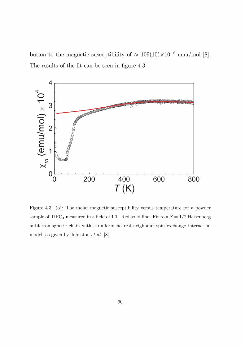
bution to the magnetic susceptibility of ≈ 109(10)×10−6 emu/mol [8].
The results of the fit can be seen in figure 4.3.
Figure 4.3: (o): The molar magnetic susceptibility versus temperature for a powder
sample of TiPO4 measured in a field of 1 T. Red solid line: Fit to a S = 1/2 Heisenberg
antiferromagnetic chain with a uniform nearest-neighbour spin exchange interaction
model, as given by Johnston et al. [8].
90

Figure 4.4: (o): Heating data. (o): Cooling data. Left: The molar magnetic sus-
ceptibility versus temperature in the region of the 74 K anomaly. Right: The molar
magnetic susceptibility versus temperature in the region of the 111 K transition.
Below ≈ 120 K, two magnetic phase transitions are indicated by two
rapid drops in the molar magnetic susceptibility at 111(1) and 74(0.5) K,
respectively, as shown in figure 4.4. The transition at 111(1) K has no
thermal hysteresis. The heating and cooling curves are identical within
experimental error. However, the transition at 74(0.5) K does exhibit a
thermal hysteresis of 50(10) mK. This can be clearly seen in figure 4.4.
91

The molar magnetic susceptibility between ≈ 105 and ≈ 80 K and below
≈ 70 K can be modelled assuming a non-magnetic ground state (which
is the case once a system undergoes a spin-Peierls transition) with a
magnetic state higher in energy. Due to thermal excitation the higher in
energy state will be slightly occupied. This assumption can be fitted to
the measured magnetic susceptibility by equation 4.1, which consists of
a S = 1/2 paramagnetic impurity, a constant temperature independent
molar magnetic susceptibility and a thermal population of a magnetic
state, ∆E above the non-magnetic ground-state.
χmol[cm3
mol] = y×
0.375[cm3K
mol ]
T[K]+χ0[
cm3
mol]+(1−y)×A[
cm3
mol]×e
−∆E[K]T[K] (4.1)
where y is the fraction of a S = 1/2 entity, χ0 is the temperature inde-
pendent magnetic susceptibility, A is a prefactor, ∆E is the energy gap
between the non-magnetic ground-state and the first magnetic excited
state and kB is the Boltzmann constant. The fitted data can be seen in
figure 4.5, with the tabulated values given in table 4.1.
It is apparent from the results listed in table 4.1 and displayed in fig-
ure 4.5, that within the two temperature ranges T ≤ ≈ 70 K and
≈ 80 ≤ T ≤ ≈ 105 K, the molar magnetic susceptibility conforms to
the aforementioned model, but in a rather different manner. Most no-
92

T ≤ ≈ 70 K ≈ 80 K ≤ T ≤ ≈ 105 K
y 8.00(1)×10−4 (v) 8.00×10⁻⁴(f)
χ0 (cm3/mol) 5.68(3)×10−5(v) 8.2(1)×10−5 (v)
A (cm3/mol) 1 (f) 0.0052(6) (v)
∆E (K) 830(10) (v) 425(15) (v)
Table 4.1: The values for the fits to the molar magnetic susceptibility displayed in
figure 4.5, the errors are given in parentheses. (v) and (f) denote a varied or fixed
quantity, respectively.
table are the different values for the excitation ∆E values which imply an
energy gap of ≈ 425 K in the high-temperature regime, but a larger gap
of≈ 830 K after the second transition, below≈ 70 K. The prefactor, A, is
not the same for both temperature ranges. Within the low-temperature
range the prefactor is 1 cm3/mol, but in the higher temperature range
the value was refined to ≈ 0.005 cm3/mol. One can clearly see that
the two different regimes can be explained assuming a non-magnetic
ground-state and a magnetic state higher in energy. However, the higher
temperature regime has a much larger van Vleck contribution than the
low-temperature regime, this implies two different energy landscapes.
This is consistent with the change in ∆E, since the van Vleck contribu-
tion is inversely proportional to the energy gap between the ground-state
and the first excited state [4]. The change in energy landscape could be
93
due to the deformation of the ligand field at ≈ 73 K. The transition
at ≈ 73 K was found to be a first order phase transition and hence
includes a structural transition. The difference in the prefactors could
be tentatively explained by describing the low-temperature regime as
a static energy landscape (non-dynamic), while the higher temperature
regime is highly dynamic and fluctuating. Due to the timescale of the
magnetic susceptibility measurements one sees an average excitation and
an average population of the excited state. This could possible explain
the very small prefactor seen for the high-temperature regime. This is
consistent with the nuclear magnetic resonance results which show the
high-temperature regime to be non-static, see section 4.7. However this
is not definitive and further experiments such as muon spin rotation will
be needed to clarify the nature of the intermediate regime further.
94

Figure 4.5: (o): The low-temperature molar magnetic susceptibility versus temperature
for TiPO4. The red and blue solid lines are fits of the data using equation 4.1 and the
values tabulated in table 4.1.
4.4 Specific heat
The specific heat of an orientated single crystal weighing 27.8 mg was
determined in the temperature range 2 K to 220 K. The specific heat
exhibits two λ-type anomalies at 110.9(0.6) and 74.1(0.3) K, see figure
95

4.6. The results are consistent with the molar magnetic susceptibility,
see section 4.3. The anomaly at low-temperature was found to exhibit a
thermal hysteresis of approximately 40(20) mK. Again no hysteresis was
seen for the high temperature anomaly, see figure 4.7.
Figure 4.6: Main (o): The specific heat versus temperature for TiPO4. Insert (o): The
specific heat divided by temperature versus temperature.
96

Figure 4.7: The specific heat of TiPO4 (o): Cooling data. (o): Heating data. Left:
The specific heat versus temperature in the region on the 74 K transition. Right: The
specific heat versus temperature in the region of the 111 K transition.
4.5 Electron paramagnetic resonance
The temperature and angular dependent electron paramagnetic reso-
nance signal was measured on an oriented 1.72 mg single crystal mounted
on a samples holder with a calibrated temperature sensor next to the
sample, see section 2.4. A single Lorentzian absorption line was ob-
97
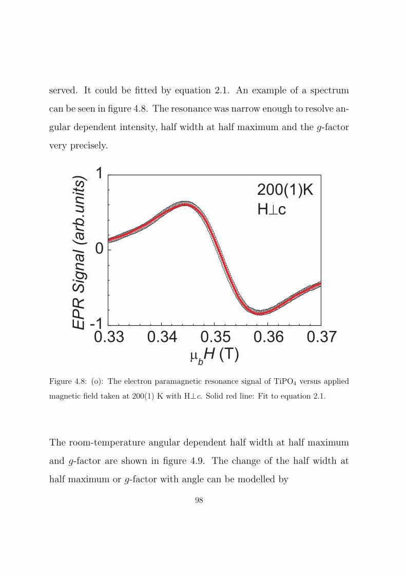
served. It could be fitted by equation 2.1. An example of a spectrum
can be seen in figure 4.8. The resonance was narrow enough to resolve an-
gular dependent intensity, half width at half maximum and the g-factor
very precisely.
0.33 0.34 0.35 0.36 0.37-1
0
1
EP
RS
ign
al(a
rb.u
nits)
mbH (T)
200(1)K
H^c
Figure 4.8: (o): The electron paramagnetic resonance signal of TiPO4 versus applied
magnetic field taken at 200(1) K with H⊥c. Solid red line: Fit to equation 2.1.
The room-temperature angular dependent half width at half maximum
and g-factor are shown in figure 4.9. The change of the half width at
half maximum or g-factor with angle can be modelled by
98
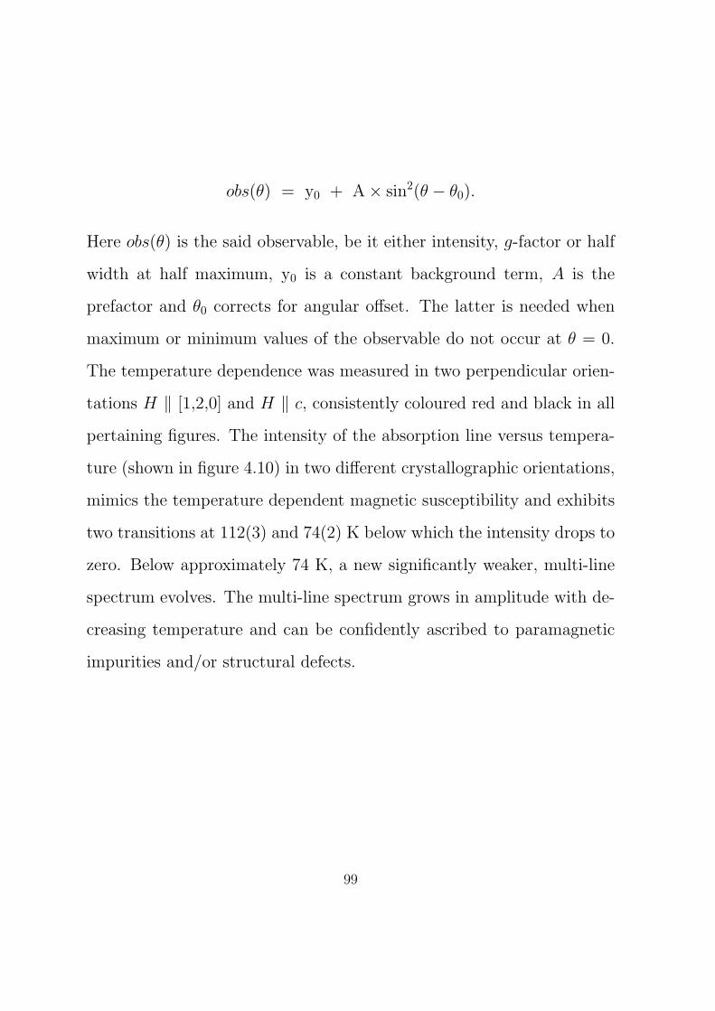
obs(θ) = y0 + A× sin2(θ − θ0).
Here obs(θ) is the said observable, be it either intensity, g-factor or half
width at half maximum, y0 is a constant background term, A is the
prefactor and θ0 corrects for angular offset. The latter is needed when
maximum or minimum values of the observable do not occur at θ = 0.
The temperature dependence was measured in two perpendicular orien-
tations H ∥ [1,2,0] and H ∥ c, consistently coloured red and black in all
pertaining figures. The intensity of the absorption line versus tempera-
ture (shown in figure 4.10) in two different crystallographic orientations,
mimics the temperature dependent magnetic susceptibility and exhibits
two transitions at 112(3) and 74(2) K below which the intensity drops to
zero. Below approximately 74 K, a new significantly weaker, multi-line
spectrum evolves. The multi-line spectrum grows in amplitude with de-
creasing temperature and can be confidently ascribed to paramagnetic
impurities and/or structural defects.
99

Figure 4.9: Fitting parameters for the electron paramagnetic resonance signal of TiPO4
at 306(1) K, versus angle of the applied magnetic field with regards to the [1,2,0]c-plane.
Solid red line: Fit to a sin2(θ) dependence. Main: The half width at half maximum.
Insert: g-factor.
As shown in figure 4.10 above 74 K the g-factor for the two selected ori-
entations (H ∥ c and H ∥ [1,2,0]) shows a mild, almost linear decrease
with increasing temperature. On closer inspection, however, an anomaly
is observed in both orientations at ≈ 110 K, consistent with other exper-
100

iments. A ≈ 0.01% decrease is apparent in the H ∥ [1,2,0], with a slight
change in temperature dependence observed for H ∥ c. Above 120 K the
half width at half maximum for both orientations are seen to increase in
a linear fashion with increasing temperature. This is in agreement with
theoretical work by Oshikawa and Affleck and similar to values found for
CuGeO3 (see section 1.2.4) [36, 37]. A linear behaviour of the half width
at half maximum at low-temperatures can be ascribed to anisotropic
anti-ferromagnetic one-dimensional spin exchange interactions. A linear
dependence of 8.48(3) × 10−4 T/K and 5.79(2) × 10−4 T/K was found
for H ⊥ chain and H ∥ chain, respectively. Their ratio
d(∆w(H⊥chain))dT
(d∆w(H∥chain))dT
≈ 1.5,
differs from the suggested ratio of 2 [36, 37]. The deviation could be
due to H ⊥ c and H ∥ c not being parallel to H ⊥ ace and H ∥ ace,
respectively, where ace is the easy plane. Due in part to the canting of
the easy axes with regards to each other i.e. there are two easy axes
which are canted away from the the crystallographic b axis slightly into
the c-axis. The ratio does, however, confirm that the easy axis is rather
more parallel to b than to c.
With decreasing temperature, below ≈ 110 K, the half width at half
101

maximums start to increase until at ≈ 100 K where they once again
start to decrease, see figure 4.10. The half width at half maximums
continue to decrease from then on, until the signal intensity drops to
zero at ≈ 74 K.
102

(a)
(b)
(c)
0 100 200 3000.0
0.5
1.0
1.5
HW
HM
(T)´
10
2
T (K)
1.92
1.93
1.94
1.95
g-f
acto
r
0
40
80
120
Inte
nsity
(arb
.uin
ts)
Figure 4.10: (o): H ∥ [1,2,0]. (o): H ∥ c. Fitted electron paramagnetic resonance
parameters of TiPO4 versus temperature (a): The intensity. (b): The g-factor. (c):
The half width at half maximum, the solid black (gradient 0.058(1) mT/K and intercept
58.2(1) K) and red (gradient 0.085(1) mT/K and intercept 59.0(1) K) lines are linear
fits to the H ∥ c and H ∥ [1,2,0] data, respectively.
103

4.6 ab initio calculations
To probe the magnetic properties of TiPO4 first principles total energy
calculations were performed†. To examine the magnetic properties of
TiPO4, the three spin exchange paths shown in figure 4.11 were consid-
ered. Subsequently the spin configuration energies were mapped onto a
Heisenberg spin exchange Hamiltonian (the same procedure described in
detail for CuCrO4, in the previous chapter);
H = −∑ij
JijSiSj.
Here, Jij is the spin exchange for the spin exchange interaction between
the spins at sites i and j, while Si and Sj are the spin angular momen-
tum operators. The Hamiltonian includes nn and nnn intra-chain spin
exchange interactions J1 and J2. Additionally, the inter-chain spin ex-
change coupling, J3, was allowed. J3 connects Ti atoms with identical y
and z coordinates, i.e. along the crystallographic a direction, see figure
4.11. The calculations of the total energies of the four ordered spin states
of TiPO4, FM, AF1, AF2, and AF3, were done on the basis of density
functional theory electronic band structure calculations. The density
†The first principle density functional theory calculations were done by Prof. M. Whangbo and
his group at North Carolina State University, Raleigh, N. C., USA.
104

functional theory calculations employed the Vienna ab initio simulation
package [59, 61, 60] with the projected augmented-wave method, the
generalized gradient approximation (GGA) for the exchange and corre-
lation functional [62]. A plane-wave cut-off energy of 400 eV was used
with a set of 56 k-points in the irreducible Brillouin zone and a threshold
of 10−5 eV for the self-consistent-field convergence of the total electronic
energy. More details can be found in Law et al. [74].
To account for electron correlations associated with the Ti 3d state, GGA
plus onsite repulsion (GGA+U ) calculations were performed with U =
2 and 3 eV for Ti [63]. The relative energies of the four ordered spin
states obtained from our GGA+U calculations are summarized in table
4.2. By mapping the relative energies of the four ordered spin states
given in terms of the spin exchange parameters, see figure 4.11, onto the
corresponding relative energies obtained from the GGA+U calculations
the spin exchange parameters J1 - J3 were found. They are summarized
in table 4.2.
105

FM (0, 0) AF1 (-42.5, -32.5)
EFM=(-J1 - J2 - J3)/4 EAF1=(+J1 - J2 - J3)/4
AF2 (-21.3, -16.3) AF3 (-43.5, -33.0)
EAF2=(+J2 - J3)/4 EAF3=(+J1 - J2 + J3)/4
J1
J2
J3
Figure 4.11: The spin exchange pathways and the four spin configurations for which
the total energy has been calculated by GGA+U calculations. Relative energies in
parentheses given in meV, first for U = 2 eV and then for U = 3 eV. Below the figures
are the equations for mapping the energies onto the aforementioned spin exchange
pathways.
Since there is a first order transition at ≈ 74 K, any group subgroup rela-
tions do not apply. Hence, one can not predict the new low-temperature
structure by systematically lowering the symmetry. So in order to probe
106

Ji U = 2 eV U = 3 eV
J1 -988 -751
J2 -1.4 +0.7
J3 -20 -15
Table 4.2: Values of the spin exchange parameters J1 - J3 (in K) for TiPO4 obtained
by mapping the GGA+U total energies of the four spin configurations, see figure. 4.11,
onto the Hamiltonian details are given in the text.
the low-temperature structure, structure optimization based on first
principles density functional theory calculations were carried out. They
started from crystal structure configurations which were slightly dis-
torted modifications of the room-temperature structure. Within the
calculations the atom positions were allowed to relax, only retaining
P1 (translation) symmetry for a supercell 2×2×2 times the Cmcm unit
cell. A dimerisation of the Ti chains with a sizeable bond alternation,
Ti· · ·Ti = 3.1737 A ± ∆ (∆ = 0.2760 A) and two different phospho-
rus environments, were observed. The resulting lowest energy structure
consisted of 48 atoms in P1 symmetry. By employing the ADDSYM
routine [79, 80] within the PLATON[81] program, hidden symmetry ele-
ments could be found and the structure reclassified. Employing this, the
lowest energy structure was found to best conform to the space group
Pmmn with a = 5.29(1) A, b = 6.34(1) A and c = 7.91(1) A. The
107

atom oxidation state Wyckoff position and letter x y z
Ti +3 4e 0.7500 0.0216 0.2437
P1 +5 2b 0.7500 -0.7500 0.8909
P2 +5 2a 0.2500 0.2500 0.4108
O1 -2 4e 0.2500 0.0470 0.5120
O2 -2 4f 0.0146 -0.7500 0.2898
O3 -2 4f -0.0038 -0.7500 0.7824
O4 -2 4e 0.2500 -0.0488 0.0003
Table 4.3: The predicted atomic parameters for TiPO4, in the space group Pmmn.
resulting atomic parameters are given in table 4.3.
The total energy of the Pmmn structure was found to be ≈ 48.26 meV
per formula unit lower than the non-relaxed room-temperature structure.
Figure 4.12 displays the interatomic distances for the TiO6 octahedron
and the PO4 tetrahedra with the Ti· · ·Ti distances, for the predicted
low-temperature structure of TiPO4.
108

Figure 4.12: Predicted interatomic distances. (a): TiO6 octahedron. (b) and (c): The
two different PO4 tetrahedra. (d): Ti· · ·Ti distances in the dimerized Ti chain.
4.7 Magic angle spinning 31P nuclear magnetic res-
onance and Raman spectroscopy measurements
Magic angle spinning 31P nuclear magnetic resonance (resonance fre-
quency 80.98 MHz) spectroscopy was undertaken on a powder TiPO4
sample‡, using a center field of ≈ 8.5 T and a spinning frequency of
≈ 25 kHz. The spectra were collected between ≈ 35 K and room-
temperature, in a continuous flow cryostat using a cryoMAS probe. The
temperature was measured with a calibrated Cernox Resistor placed a
‡The magic angle spinning nuclear magnetic resonance was done by Prof. I. Heinmaa and Dr. R.
Stern at the National Institute of Chemical Physics and Biophysics, Estonia.
109
fixed distance away from the sample. The distance resulted in the sample
temperature being approximately 5% higher than the measured tem-
perature, which was later corrected for. Above ≈ 140 K a single 31P
symmetric nuclear magnetic resonance line accompanied by two sets of
very weak symmetrically placed spinning sidebands was observed. The
spectra are displayed in descending temperature in figure 4.13. Near
112 K the line becomes distorted and broadens into a highly asymmetric
continuum limited by two boundary peaks. With decreasing tempera-
ture the continuum continues to expands, until it finally washes out at
≈ 76 K, whereupon the lower boundary grows and finally consists of
two symmetric equally intense lines. Each line is accompanied by two
sets of symmetric spinning sidebands. The peak positions and/or the
boundary edges are displayed versus temperature in figure 4.14. The
onset of the two 31P lines, at ≈ 76 K is in good agreement with the
transition temperatures found by specific heat and molar magnetic sus-
ceptibility measurements. The occurrence of two 31P lines results from
two different PO4 tetrahedra. This is consistent with the predicted new
low-temperature structure from density functional theory calculations.
The structural distortion that would result in two different PO4 tetra-
hedra would also distort the TiO6 octahedra, resulting in two different
TiO6 environments and possible two different Ti3+· · ·Ti3+ bond lengths.
110
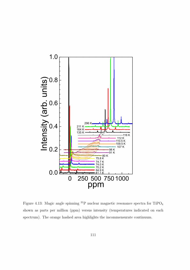
0 250 500 75010000.0
0.2
0.4
0.6
0.8
1.0
In
tens
ity (a
rb. u
nits
)
ppm
116 K112 K
110.5 K109.5 K107 K
98 K91 K
80 K75.8 K74.7 K74.0 K70.2 K64.9 K41.1 K
296 K211 K164 K135 K
Figure 4.13: Magic angle spinning 31P nuclear magnetic resonance spectra for TiPO4
shown as parts per million (ppm) versus intensity (temperatures indicated on each
spectrum). The orange hashed area highlights the incommensurate continuum.
111
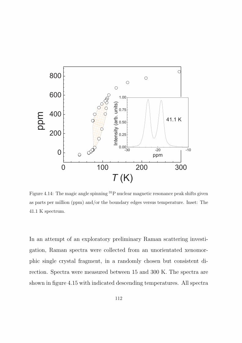
0 100 200 300
0
200
400
600
800
pp
m
T (K)
-30 -20 -100.00
0.25
0.50
0.75
1.00
Inte
nsity
(arb
.u
nits)
ppm
41.1 K
Figure 4.14: The magic angle spinning 31P nuclear magnetic resonance peak shifts given
as parts per million (ppm) and/or the boundary edges versus temperature. Inset: The
41.1 K spectrum.
In an attempt of an exploratory preliminary Raman scattering investi-
gation, Raman spectra were collected from an unorientated xenomor-
phic single crystal fragment, in a randomly chosen but consistent di-
rection. Spectra were measured between 15 and 300 K. The spectra are
shown in figure 4.15 with indicated descending temperatures. All spectra
112

shown here were measured with a green laser (λ = 532 nm). The room-
temperature spectrum consists of 13 modes. The CrVO4 structure-type
should exhibit as many as 15 Raman active modes according to sym-
metry analysis, 5 Ag modes, 4 B1g modes, 2 B2g and 4 B3g [82]. The 2
missing modes could be due to a combination of several of the following
reasons:
Accidental degeneracy where they occur at the same wave number as
other peaks and therefore they can not be seen.
Zero intensity of the two missing peaks due to a small, effectively zero,
coupling constant.
Lastly their absence could be explained because they may have low in-
tensity in the direction of observation. This would imply that in another
orientation they would be visible.
Between 300 and 125 K the spectra are practically identical, with only
a small shift of position (≈ 0.2%) and narrowing (≈ 30%) of the peaks.
113

0 200 400 600 1000 1200
300 K
25 K
In
tens
ity (a
rb. u
nits
)
Wavenumber (cm-1)
15 K
81 K77 K73 K69 K
93 K89 K85 K
109 K105 K101 K97 K
65 K55 K45 K35 K
121 K117 K113 K
275 K250 K225 K200 K175 K150 K125 K
Figure 4.15: Raman spectra of a TiPO4 crystal collected in an arbitrary and constant
orientation. The data are displayed in descending temperature as indicated. The x-axis
is broken between 700 and 900 cm−1.
114

0 200 400 600 800 1000 1200
*** *
***
*
*
*
*
*
In
tens
ity (a
rb. u
nits
)
Wavenumber (cm-1)
*
Figure 4.16: The room-temperature and the (offset) 15 K Raman spectra, red and
black, respectively. In the 15 K spectrum new peaks are indicated by asterisks.
115

Figure 4.17: (o) and (o): Two new low-temperature regime Raman modes, centered at
≈ 231 cm−1 and ≈ 400 cm−1, respectively. Upper: The development of the full width
at half maximum for both modes versus temperature. Lower: The integrated intensity
of the two modes versus temperature. Blue solid line: Fit to both data sets, with Tc
= 125(1) K and β = 0.28(3). Inset: A different representation of the lower figure on a
log-log plot, with 1-T/Tc as the x-axis rather than temperature. The solid blue line is
the fitted line from the lower figure.
Below ≈ 125 K, 12 new peaks start to grow out of the background. They
continue to increase in intensity with descending temperature until ≈ 75
K, whereupon their intensity stays relatively constant with descending
116

temperature. It should be noted that the predicted low-temperature
structure is expected to exhibit a maximum of 36 Raman active modes.
The 300 and 15 K spectra are illustrated in figure 4.16 for comparison.
The development of two new low-temperature modes with descending
temperature is shown in figure 4.17, the integrated intensity, I, was
fitted to a critical power law such as, I(T ) ∝ (1− ( TTc))2β, yielding a crit-
ical exponent of 0.28(3) and a transition temperaure, Tc, of 125(1) K. All
modes display a relatively constant width and intensity below ≈ 75 K,
but a slight shift (≈ 0.05%) of position to smaller wavenumbers is re-
solved between ≈ 125 K and the lowest-temperature. A more detailed
Raman scattering investigation of TiPO4 is underway.
4.8 Low-temperature diffraction
Single crystal x-ray diffraction patterns § were collected between room-
temperature and 93 K, using the STOE STADI-I, from a xenomorphic
fragment of TiPO4. After correction for absorption effects the integrated
intensities were refined. Down to 93 K the crystal structure remained
isostructural to that reported previously for the room-temperature struc-
ture [73]. The lattice constants and atomic positions were followed as a
§The single crystal structure determination has been done in collaboration with Dr. C. Hoch,
MPI-FKF Stuttgart, Germany.
117

function of temperature. The unit cell volume, V , and lattice constants
a, b and c are displayed versus temperature in figure 4.18. Between
room-temperature and ≈ 110 K the a and b lattice constants increase
with decreasing temperature by ≈ 0.15% and ≈ 0.07%, respectively. The
c lattice constant decreases with temperature within the same range by
≈ 0.25%. As a result the volume is seen to stay relatively constant.
The volume thermal expansion; α = 1V0
∂V (T )∂T amounts to ≈ 2×10⁻⁶ K−1,
comparable to that of low thermal expansion materials such as diamond,
which has a coefficient of thermal expansion of ≈ 1×10⁻⁶ K−1 at room-
temperature [83].
118

5.268
5.272
5.276
5.280a
(Å
)
7.864
7.868
7.872
7.876
b(Å
)
6.28
6.29
6.30
6.31
c(Å
)
50 100 150 200 250 300260.5
261.0
261.5
262.0
T (K )
V(Å
3)
(a)
(b)
(c)
(d)
Figure 4.18: Results of the refinement of the single crystal diffraction patterns of TiPO4,
solid lines are a guide for the eye. (a) The a lattice parameter versus temperature.
(b) The b lattice parameter versus temperature. (c) The c lattice parameter versus
temperature. (d) The volume of the unit cell versus temperature.
119

The quality of the investigated crystal proved to be exemplary. As
such the residual electron density as a function of temperature could
be followed. Comparing the calculated electron density, based upon a
spherical model, with those ascertained from our single crystal diffrac-
tion patterns, considerable residual electron density was found located
within the ac-plane adjacent to the Ti atom. The residual electron den-
sity was mainly confined to four pockets (two pairs). One such pair
was situated on opposite sides of the Ti atom in an interstitial position
in the ribbon chain. The second pair was again on opposite sides of
the Ti atom but perpendicular to the ribbon chain. Due to the sym-
metry of the structure within the pairs, the pockets must have equal
intensity. At room-temperature the residual electron density of the two
pairs appears approximately equally occupied. Upon cooling there was
a gradual migration of the density away from the perpendicular pair into
the interstitial pair. This change is complemented by a reduction in the
Ti· · ·Ti distance by ≈ 0.5% and a similar reduction in the angle of the
nn superexchange pathway by ≈ 0.4%. The development of the residual
electron density with decreasing temperature is displayed in figure 4.19.
120

Figure 4.19: The residual electron densities, obtained from single crystal structure
refinements of TiPO4, at different temperatures. The temperatures are indicated on
the right hand side.
In order to probe the low-temperature structure, a neutron powder
121
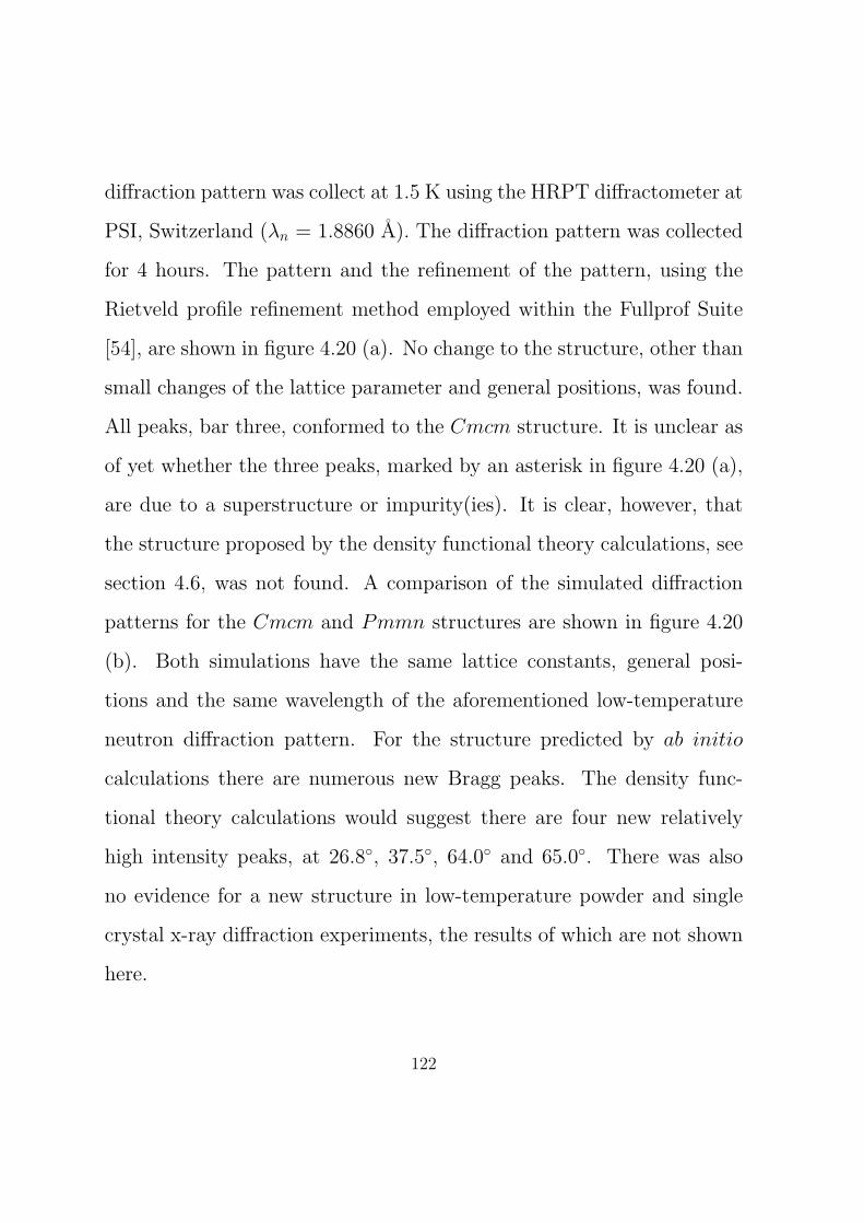
diffraction pattern was collect at 1.5 K using the HRPT diffractometer at
PSI, Switzerland (λn = 1.8860 A). The diffraction pattern was collected
for 4 hours. The pattern and the refinement of the pattern, using the
Rietveld profile refinement method employed within the Fullprof Suite
[54], are shown in figure 4.20 (a). No change to the structure, other than
small changes of the lattice parameter and general positions, was found.
All peaks, bar three, conformed to the Cmcm structure. It is unclear as
of yet whether the three peaks, marked by an asterisk in figure 4.20 (a),
are due to a superstructure or impurity(ies). It is clear, however, that
the structure proposed by the density functional theory calculations, see
section 4.6, was not found. A comparison of the simulated diffraction
patterns for the Cmcm and Pmmn structures are shown in figure 4.20
(b). Both simulations have the same lattice constants, general posi-
tions and the same wavelength of the aforementioned low-temperature
neutron diffraction pattern. For the structure predicted by ab initio
calculations there are numerous new Bragg peaks. The density func-
tional theory calculations would suggest there are four new relatively
high intensity peaks, at 26.8◦, 37.5◦, 64.0◦ and 65.0◦. There was also
no evidence for a new structure in low-temperature powder and single
crystal x-ray diffraction experiments, the results of which are not shown
here.
122
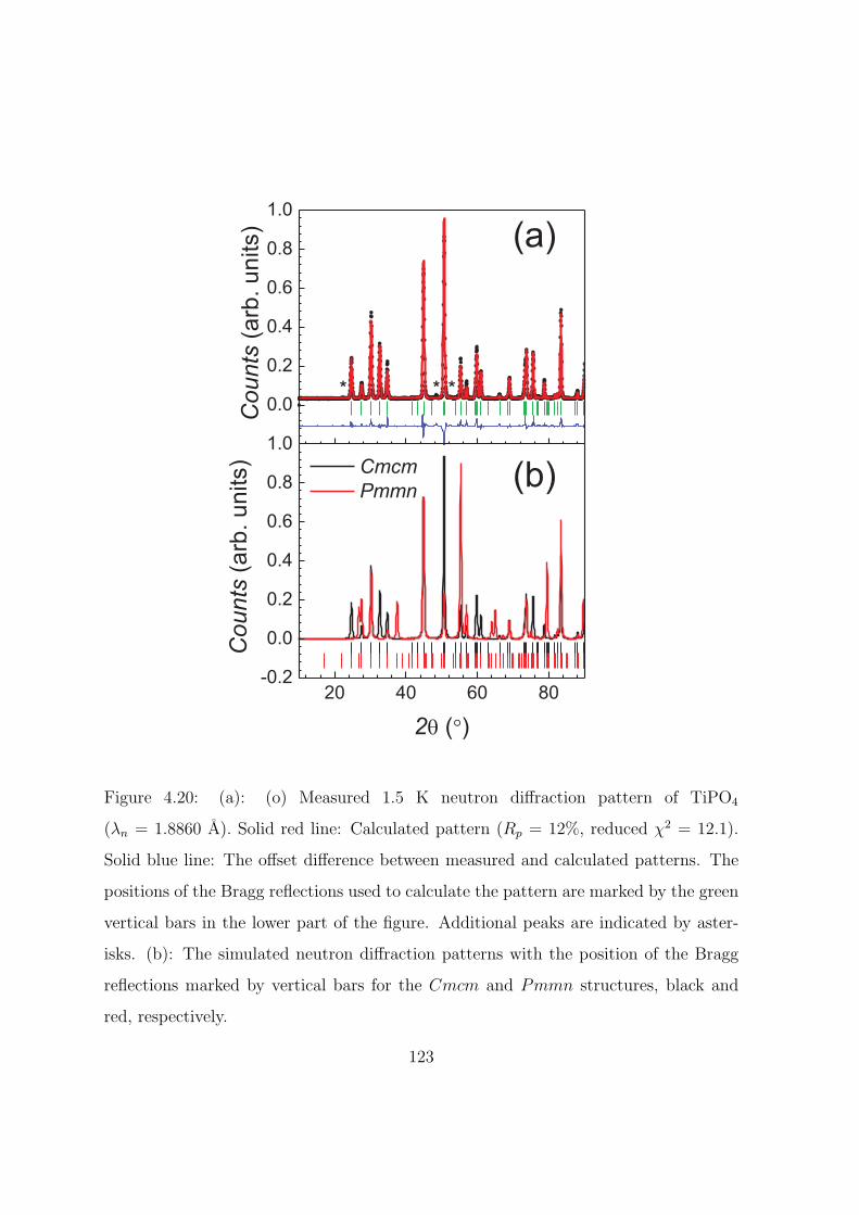
Figure 4.20: (a): (o) Measured 1.5 K neutron diffraction pattern of TiPO4
(λn = 1.8860 A). Solid red line: Calculated pattern (Rp = 12%, reduced χ2 = 12.1).
Solid blue line: The offset difference between measured and calculated patterns. The
positions of the Bragg reflections used to calculate the pattern are marked by the green
vertical bars in the lower part of the figure. Additional peaks are indicated by aster-
isks. (b): The simulated neutron diffraction patterns with the position of the Bragg
reflections marked by vertical bars for the Cmcm and Pmmn structures, black and
red, respectively.
123

4.9 Discussion and conclusion
In this chapter it was shown that at high-temperatures TiPO4 is an ex-
ceptionally strongly coupled one-dimensional Heisenberg anti-ferromagnet.
The magnetic susceptibility of TiPO4 exhibits a broad hump in the mag-
netic susceptibility that could be fitted to a uniform non-alternating
S = 1/2 chain, with Jnn ≈ -970 K. The very large superexchange is
confirmed by density functional theory calculations that show TiPO4 to
have a nn spin exchange interactions of ≈ -970 K with a small effectively
zero nnn spin exchange interaction. Laboratory based x-ray diffraction
at room-temperature confirmed the crystal structure to be of the CrVO4
structure-type. Ab initio density functional calculations suggest that
at lower temperatures TiPO4 should undergo long-range ordering via
inter-chain coupling.
At 111 K an anomaly is seen in specific heat, magnetic susceptibility and
electron paramagnetic resonance measurements. The anomaly is second
or high order (it exhibits no thermal hysteresis) and is reminiscent of
those seen in TiOHal [28, 29, 30, 31, 32, 33]. Below 111 K the magnetic
susceptibility can be explained by a thermal population of a magnetic
state higher in energy than the non-magnetic ground state. Below 111 K
new Raman peaks are visible, indicating a new crystal structure. Magic
124
angle spinning 31P nuclear magnetic resonance confirms the transition
at 111 K and shows a broad continuum of nuclear magnetic resonance
intensity indicative of an incommensurate structure. However, at 90 K
low-temperature x-ray diffraction does not show a new crystal structure.
At lower temperatures still, 74 K, a second anomaly is seen in the mag-
netic susceptibility, specific heat and electron paramagnetic resonance
which is hysteretic, hence first order in nature. At this point the broad
continuum seen in nuclear magnetic resonance washes out to leave two
31P peaks of equal intensity, unequivocally showing that there is a new
crystal structure. The magnetic susceptibility is still explainable by a
thermal population of a magnetic state above a non-magnetic ground
state but the gap is much larger. The electron paramagnetic resonance
signal intensity falls fully to zero. This is clear evidence for a non-
magnetic ground-state.
The observed phase transitions are interpreted as a two part spin-Peierls
transition, where between 111 and 74 K TiPO4 is in a dynamically fluc-
tuating spin-Peierls state. Below 74 K the spin-Peierls phase becomes
static and a new dimerised phase should exist. The new low-temperature
structure has been predicted by ab initio calculations, but neither this
structure nor any other new structure have been observed in a 1.5 K
high intensity powder neutron diffraction experiment. However, the new
125

structure predicted by ab initio calculations could quite possible be in-
correct, since the calculations could have converged to a local, rather
than the global, energy minimum. Future experiments are planned to
search for superstructure reflections. They will involve using high resolu-
tion powder neutron diffraction to search for peak splitting which might
not have been seen in the 1.5 K experiment.
In conclusion, there is overwhelming evidence from molar magnetic sus-
ceptibility, electron paramagnetic resonance and magic angle spinning
31P nuclear magnetic resonance measurements that TiPO4 has a non-
magnetic ground-state. There is a confirmed, unknown, new static
low-temperature structure below ≈ 74 K, as evidenced by specific heat
and nuclear magnetic resonance measurements, Raman scattering and
ab inito calculations. Within this new structure there is strong evi-
dence that there are two different phosphorus environments and a bond-
alternation within the Ti· · ·Ti chains. However, no diffraction exper-
iment has shown a new structure, as of yet. Within the temperature
range of 110.9(0.6) > T > ≈ 74.1(0.3) K a non-magnetic possible dy-
namic state exists. At high-temperatures TiPO4 can be described by
a S=1/2 Heisenberg anti-ferromagnetic chain with a nn exchange of
≈ 970 K.
126

4.10 Summary
In the preceding chapter it was shown that there is strong evidence
from magnetic susceptibility, electron paramagnetic resonance, nuclear
magnetic resonance and specific heat measurements that TiPO4 might
undergo a two-stage spin-Peierls transition. However, lab based x-ray
diffraction at 90 K and powder neutron diffraction at 1.5 K do not show
a new structure, in either the intermediate or low-temperature phase.
TiPO4 has the highest spin-Peierls transition temperature known to
date. However, there still remain some unanswered questions. If there
is a spin-Peierls transition what is the new structure at low-temperature
and does the spin-Peierls transition move with the application of a mag-
netic field? In order to answer these questions and definitively prove that
TiPO4 undergoes a spin-Peierls transition further experiments should
complement our exploratory investigation.
In the final chapter, I will summarize the work reported in this PhD
thesis and address some outstanding questions.
127

Chapter 5
Conclusion
In my PhD thesis I report a theoretical effort of establishing a Pade
approximation for the description of the temperature dependence of a
S = 3/2 non-alternating spin chain. The approximation can be used as a
handy tool for researchers and can be modelled against their data. How-
ever, this approximation is not yet tested against a real system. This
work could be continued by extending the calculations to higher reduced
temperature and modelling against known compounds. Expanding fur-
ther, similar calculations could be done for other spin systems, such as
S = 1, 2 and 5/2. It could also be extended to include the larger mag-
netic moments of the rare earth atoms e.g. Gd3+, Eu2+ with S = 7/2.
However, there would not be a significant improvement over the classical
approximation.
128

In the first experimental chapter the preparation and characterization
of CuCrO4 was discussed, the results were supported by ab initio cal-
culations. CuCrO4 was characterized by molar magnetic susceptibil-
ity, electron paramagnetic resonance, specific heat and dielectric con-
stant measurements. Experimental results show clear indication for one-
dimensional magnetism with long-range ordering at ≈ 8.2 K which is ac-
companied by a dielectric anomaly. The temperature dependent molar
magnetic susceptibility could be modelled against a nearest-neighbour
and next nearest-neighbour nnn S = 1/2 Heisenberg spin chain with
Jnn/Jnnn ≈ 2. Theoretical calculations support the ratio of Jnn/Jnnn be-
ing close to 2, putting CuCrO4 in the vicinity of the Majumdar-Ghosh
point. CuCrO4 was found to be a new type-II multiferroic system.
Future high magnetic field measurements are planned in order to con-
firm the prediction of magnetization plateaus at low-temperatures. Ad-
ditionally, high intensity neutron diffraction experiments are scheduled
to confirm long-range magnetic ordering, to establish the magnetic struc-
ture and to confirm the spin spiral structure. High resolution neutron
diffraction experiments are planned to follow the structural parameters
as a function of temperature and to probe the shallow double maximum
seen in the dielectric constant measurements. Furthermore muon spin
rotation experiments are planned to investigate the possibility of long-
129
range magnetic ordering, 53Cr nuclear magnetic resonance measurements
are scheduled to probe the possible incommensurate magnetic structure.
However, the most pressing concern is the growth of single crystals, since
with them it would be possible to investigate in more detail ferroelec-
tricity by measuring a ferroelectric polarization loop.
In the fourth chapter of my PhD thesis the experimental and theoret-
ical characterization of TiPO4 was reported. Single crystal of TiPO4
were grown by chemical vapor transport, these were then characterized
by molar magnetic susceptibility, electron paramagnetic resonance and
specific heat measurements. Additionally low-temperature single crystal
and powder diffraction was carried out, using x-ray and neutron radia-
tion. TiPO4 was found to have a two stage spin-Peierls transition with an
exceptionally high transition temperature. At ≈ 111 K TiPO4 undergoes
a transition into a dynamically dimerised phase. At lower temperatures
still, ≈ 74 K, TiPO4 passes through a first order phase transition into
a fully dimerised phase. There is overwhelming evidence for a new low-
temperature structure, but as of yet this has not been confirmed. In
the near future I am planning to measure low-temperature single crys-
tal neutron diffraction patterns of TiPO4 in order to investigate a new
low-temperature structure. I plan to follow this up by collecting high res-
olution powder neutron diffraction patterns at 4.2 K. High magnetic field
130

measurements are also planned in order to; firstly search for a magnetic
field induced magnetic state at low-temperatures, and secondly to probe
whether the two phase transitions move with the application of a large
magnetic field. Additionally I intend to determine the spin gap in TiPO4
via muon spin rotation, which is excepted to be more accurate than nu-
clear magnetic resonance or magnetic susceptibility measurements.
131

Bibliography
[1] Coey, J. M. D. Magnetism and magnetic materials. Cambridge
Univerisity Press, (2009).
[2] Blundell, S. Magnetism in condensed matter physics. Oxford Uni-
verisity Press, (2001).
[3] Skomski, R. Simple models of magnetism. Oxford graduate texts,
(2008).
[4] Kittel, C. Indroduction to Solid State Physics - 8th Edition. John
Wiley and Sons, Inc., (2004).
[5] Mostovoy, M. Physical Review Letters 96(6), 067601 (2006).
[6] Sergienko, I. A. and Dagotto, E. Physical Review B 73(9), 094434
(2006).
[7] Mermin, N. D. and Wagner, H. Physical Review Letters 17(22),
1133 (1966).
132
[8] Johnston, D. C., Kremer, R. K., Troyer, M., Wang, X., Klumper,
A., Bud’ko, S. L., Panchula, A. F., and Canfield, P. C. Physical
Review B 61(14), 9558 (2000).
[9] van den Brink, J. and Khomskii, D. I. Journal of Physics: Con-
densed Matter 20(43), 434217 (2008).
[10] Dos Santos, A. M., Parashar, S., Raju, A. R., Zhao, Y. S.,
Cheetham, A. K., and Rao, C. N. R. Solid State Communications
122(1–2), 49 (2002).
[11] Belik, A. A., Azuma, M., Saito, T., Shimakawa, Y., and Takano, M.
Chemistry of Materials 17(2), 269 (2005).
[12] Khomskii, D. I. Journal of Magnetism and Magnetic Materials
306(1), 1 (2006).
[13] Cheong, S.-W. and Mostovoy, M. Nature Materials 6(1), 13 (2007).
[14] Katsura, H., Nagaosa, N., and Balatsky, A. V. Physical Review
Letters 95(5), 057205 (2005).
[15] Majumdar, C. K. and Ghosh, D. K. Journal of Mathematical
Physics 10(8), 1388 (1969).
[16] Majumdar, C. K. and Ghosh, D. K. Journal of Mathematical
Physics 10(8), 1399 (1969).
133

[17] Bursill, R., Gehring, G. A., Farnell, D. J. J., Parkinson, J. B., Xiang,
T., and Zeng, C. Journal of Physics: Condensed Matter 7(45), 8605
(1995).
[18] Tonegawa, T. and Harada, I. Journal of the Physical Society of
Japan 56(6), 2153 (1987).
[19] Koo, H.-J., Lee, C., Whangbo, M.-H., McIntyre, G. J., and Kremer,
R. K. Inorganic Chemistry 50(8), 3582 (2011).
[20] Banks, M. G., Kremer, R. K., Hoch, C., Simon, A., Ouladdiaf, B.,
Broto, J. M., Rakoto, H., Lee, C., and Whangbo, M.-H. Physical
Review B 80(2), 024404 (2009).
[21] Tsirlin, A. A. and Rosner, H. Physical Review B 81(2), 024424
(2010).
[22] Moeller, A., Schmitt, M., Schnelle, W., Foerster, T., and Rosner,
H. Physical Review B 80(12), 125106 (2009).
[23] Enderle, M., Mukherjee, C., Fak, B., Kremer, R. K., Broto, J. M.,
Rosner, H., Drechsler, S. L., Richter, J., Malek, J., Prokofiev, A.,
Assmus, W., Pujol, S., Raggazzoni, J. L., Rakoto, H., Rheinstadter,
M., and Ronnow, H. M. Europhysics Letters 70(2), 237 (2005).
134

[24] Law, J. M., Reuvekamp, P. G., Glaum, R., Lee, C., Kang, J.,
Whangbo, M.-H., and Kremer, R. K. accepted by Physical Review
B, April (2011).
[25] Gibson, B. J., Kremer, R. K., Prokofiev, A. V., Assmus, W., and
McIntyre, G. J. Physica B: Condensed Matter 350(1–3, Suppl. 1),
E253 (2004).
[26] Schrettle, F., Krohns, S., Lunkenheimer, P., Hemberger, J.,
Buttgen, N., Von Nidda, H. A. K., Prokofiev, A. V., and Loidl,
A. Physical Review B 77(14), 144101 (2008).
[27] Seki, S., Kurumaji, T., Ishiwata, S., Matsui, H., Murakawa, H.,
Tokunaga, Y., Kaneko, Y., Hasegaw, T., and Tokura, Y. Physical
Review B 82(6), 064424 (2010).
[28] Seidel, A., Marianetti, C., Chou, F., Ceder, G., and Lee, P. Physical
Review B 67(2), 020405 (2003).
[29] Shaz, M., van Smaalen, S., Palatinus, L., Hoinkis, M., Klemm, M.,
Horn, S., and Claessen, R. Physical Review B 71(10), 100405 (2005).
[30] Lemmens, P., Choi, K., Valenti, R., Saha-Dasgupta, T., Abel, E.,
Lee, Y., and Chou, F. New Journal of Physics 7, 74 (2005).
135
[31] Krimmel, A., Strempfer, J., Bohnenbuck, B., Keimer, B., Hoinkis,
M., Klemm, M., Horn, S., Loidl, A., Sing, M., Claessen, R., and
Zimmermann, M. V. Physical Review B 73(17), 172413 (2006).
[32] van Smaalen, S., Palatinus, L., and Schonleber, A. Physical Review
B 72(2), 020105 (2005).
[33] Ruckamp, R., Baier, J., Kriener, M., Haverkort, M. W., Lorenz, T.,
Uhrig, G. S., Jongen, L., Moller, A., Meyer, G., and Gruninger, M.
Physical Review Letters 95(9), 097203 (2005).
[34] Schoenleber, A., Shcheka, G., and van Smaalen, S. Physical Review
B 77(9), 094117 (2008).
[35] Yasuda, C., Todo, S., Hukushima, K., Alet, F., Keller, M., Troyer,
M., and Takayama, H. Physical Review Letters 94(21), 217201
(2005).
[36] Oshikawa, M. and Affleck, I. Physical Review Letters 82(25), 5136
(1999).
[37] Oshikawa, M. and Affleck, I. Physical Review B 65(13), 134410
(2002).
[38] Kubo, R. and Tomita, K. Journal of the Physical Society of Japan
9(6), 888 (1954).
136

[39] Grossjohann, S. N. PhD thesis, Technische Universitat Braun-
schweig, (2010).
[40] Hiller, W., Strahle, J., Datz, A., Hanack, M., Hatfield, W. E., Ter-
haar, L. W., and Gutlick, P. Journal of the American Chemical
Society 106(2), 329 (1984).
[41] Fischer, M. E. American Journal of Physics 32(5), 343 (1964).
[42] Stoe. IPDS Manual. Version 2.75. Stoe & Cie, (1996).
[43] http://sinq.web.psi.ch/sinq/instr/hrpt/index.html, 02 May (2011).
[44] Selwood, P. W. Magnetochemistry. Interscience, (1956).
[45] Banks, M. G. Doctoral thesis, Loughborough University, (2007).
[46] http://alps.comp-phys.org/mediawiki/index.php, 03 May (2011).
[47] http://todo.ap.t.u1tokyo.ac.jp/en/projects/alps-looper, 03 May
(2011).
[48] Loh, E. Y., Gubernatis, J. E., Scalettar, R. T., White, S. R.,
Scalapino, D. J., and Sugar, R. L. Physical Review B 41(13), 9301
(1990).
[49] Brandt, K. Arkiv for kemi, mineralogi och geologi 17A(15), 1 (1943).
137
[50] Seferiadis, N. and Oswald, H. R. Acta Crystallographica Section C
43(1), 10 (1987).
[51] Hanic, F., Horvath, I., Plesch, G., and Galikova, L. Journal of Solid
State Chemistry 59(2), 190 (1985).
[52] ScienceLab.com. online, 06 May (2011).
[53] Arsene, J., Lenglet, M., Erb, A., and Granger, P. Revue de Chimie
Minerale 15(4), 318 (1978).
[54] Rodrıguez-Carvajal, J. Physica B: Condensed Matter 192(1–2), 55
(1993).
[55] Heidrich-Meisner, F., Honecker, A., and Vekua, T. Physical Review
B 74(2), 020403 (2006).
[56] DeJongh, L. J. and Miedema, A. R. Advanves in Physics 23(1), 1
(1974).
[57] Martin, D. H. Magnetism in Solids. The M.I.T. Press, (1967).
[58] Yamada, I., Nishi, M., and Akimitsu, J. Journal of Physics: Con-
densed Matter 8(15), 2625 (1996).
[59] Kresse, G. and Hafner, J. Physical Review B 47(1), 558 (1993).
[60] Kresse, G. and Furthmuller, J. Computational Materials Science
6(1), 15 (1996).
138

[61] Kresse, G. and Furthmuller, J. Physical Review B 54(16), 11169
(1996).
[62] Perdew, J. P., Burke, K., and Ernzerhof, M. Physical Review Letters
77(18), 3865 (1996).
[63] Dudarev, S. L., Botton, G. A., Savrasov, S. Y., Humphreys, C. J.,
and Sutton, A. P. Physical Review B 57(3), 1505 (1998).
[64] Whangbo, M.-H., Koo, H. J., and Dai, D. Journal of Solid State
Chemistry 176(2), 417 (2003).
[65] Koo, H.-J. and Whangbo, M.-H. Inorganic Chemistry 47(1), 128
(2008).
[66] Koo, H.-J. and Whangbo, M.-H. Inorganic Chemistry 47(11), 4779
(2008).
[67] Kang, J., Lee, C., Kremer, R. K., and Whangbo, M.-H. Journal of
Physics-Condensed Matter 21(39), 392201 (2009).
[68] Koo, H.-J. and Whangbo, M.-H. Inorganic Chemistry 49(20), 9253
(2010).
[69] Carlin, R. L. Magnetochemistry. Springer-Verlag Berlin, Heidelberg,
New York and Tokyo, (1986).
139

[70] Schrettle, F., Krohns, S., Lunkenheimer, P., Hemberger, J.,
Buttgen, N., Krug von Nidda, H.-A., Prokofiev, A. V., and Loidl,
A. Physical Review B 77(14), 144101 (2008).
[71] Kremer, R. K. Private communication, (2011).
[72] Whangbo, M.-H. Private communication, (2011).
[73] Glaum, R. and Gruehn, R. Zeitschrift fur Kristallographie 198(1-2),
41 (1992).
[74] Law, J. M., Hoch, C., Glaum, R., Heinmaa, I., Stern, R., Kang, J.,
Lee, C., Whangbo, M.-H., and Kremer, R. K. Physical Review B
83(18), 180414 (2011).
[75] Kinomura, N., Muto, F., and Koizumi, M. Journal of Solid State
Chemistry 45(2), 252 (1982).
[76] Glaum, R., Reehuis, M., Stusser, N., Kaiser, U., and Reinauer, F.
Journal of Solid State Chemistry 126(1), 15 (1996).
[77] Yamauchi, T. and Ueda, Y. Journal of Magnetism and Magnetic
Materials 177(Part 1), 705 (1998).
[78] Glaum, R. and Gruehn, R. Zeitschrift fur Anorganishe und Allge-
meine Chemie 580(1), 78 (1990).
[79] LePage, Y. Journal of Applied Crystallography 20(3), 264 (1987).
140

[80] LePage, Y. Journal of Applied Crystallography 21(6), 983 (1988).
[81] Spek, A. L. Journal of Applied Crystalgraphy 36(Part 1), 7 (2003).
[82] Kroumova, E., Aroyo, M. I., Perez-Mato, J. M., Kirov, A., Capillas,
C., Ivantchev, S., and Wondratschek, H. Phase Transitions 76(1-2,
Part B), 155 (2003).
[83] Touloukian, Y. S., Kirby, R. K., Taylor, R. E., and Lee, T. Y. R.
Thermophysical Properties of Matter vol. 13, Thermal Expansion of
Nonmetallic Solids. Plenum, (1977).
141

Acknowledgements
Throughout the course of my PhD work I am thankful to the following
people:
Firstly my wife Bianca and my daughter Amelia for their understanding,
their patience and their support.
The rest of my family for their encouragement and continuous taunts
about my nerdy-ness.
Dr. Reinhard Kremer for his support and supervision as my supervisor
at the MPI for Solid State Research in Stuttgart.
Dr. Klaus Neumann for his supervision and for making it possible to
undertake my PhD work at the Max-Planck-Institute for Solid State
Research.
Patrick Reuvekamp for this help and encouragement throughout my PhD
work and allowing me to vent in his direction on an almost daily basis.
Dr. Jianwei Tong and Prof. Jun Sung Kim for assistance, guidance and
helpful comments throughout my research.
Dr. Constantin Hoch for countless single crystal orientations, solving
many crystal structures and for putting up with my questions.
Prof. Robert Glaum for allowing me to visit his group in order to prepare
142

samples and for supplying all other samples used.
Prof. Mike Whangbo for helpful discussions and very fruitful collabora-
tions.
Dr. Martin Rotter for instructing me in McPhas and showing an interest
in my PhD work.
Prof. Raivo Stern and Dr. Ivo Heinmaa for nuclear magnetic resonance
measurements and interest in my research.
The members of Chemistry Service and Prof. Simon’s department for
experimental assistance. However, with hindsight a lone-wolf approach
to my experimental work might have been better.
I would like to thank the computer service group and Linas Vilciauskas
for help in setting up ALPS amongst other things.
Generally many thanks to all departments in Stuttgart for assistance, if
given.
Dr. Thomas Hansen, Dr. Ines Puente Orench, Dr. Enderle Mechthild,
Dr. Bachir Ouladdiaf and Dr. Vladimir Pomjakushin for their assistance
with elastic and inelastic neutron experiments throughout my PhD work.
Dr. Hubertus Luetkens and Miss. Gwendolyne Pascua for their help
and support with muon spin rotation experiments at the PSI.
143

Finally I would like to thank all the people I have shared coffee with
in my three years at Stuttgart, most notable Linas Vilciauskas, Seth
White and Ivan Pentegov, with whom a many insightful conversations
were had.
144