identification of time-varying cable tension forces based...

STRUCTURAL CONTROL AND HEALTH MONITORINGStruct. Control Health Monit. 2017; 24: e1889Published online 29 May 2016 in Wiley Online Library (wileyonlinelibrary.com). DOI: 10.1002/stc.1889

Identification of time-varying cable tension forces based on adaptivesparse time-frequency analysis of cable vibrations

Yuequan Bao1,2,3,*,†, Zuoqiang Shi4, James L. Beck1, Hui Li2,3 and Thomas Y. Hou1

1Computing and Mathematical Sciences, California Institute of Technology, Pasadena, CA 91125, USA2Key Lab of Structures Dynamic Behavior and Control of the Ministry of Education, Harbin Institute of Technology, Harbin

150090, China3School of Civil Engineering, Harbin Institute of Technology, Harbin 150090, China

4Mathematical Sciences Center, Tsinghua University, Beijing 100084, China

SUMMARY

For cable bridges, the cable tension force plays a crucial role in their construction, assessment and long-termstructural health monitoring. Cable tension forces vary in real time with the change of the moving vehicleloads and environmental effects, and this continual variation in tension force may cause fatigue damage of acable. Traditional vibration-based cable tension force estimation methods can only obtain the time-averagedcable tension force and not the instantaneous force. This paper proposes a new approach to identify thetime-varying cable tension forces of bridges based on an adaptive sparse time-frequency analysis method. Thisis a recently developed method to estimate the instantaneous frequency by looking for the sparsesttime-frequency representation of the signal within the largest possible time-frequency dictionary (i.e. set ofexpansion functions). In the proposed approach, first, the time-varying modal frequencies are identified fromacceleration measurements on the cable, then, the time-varying cable tension is obtained from the relationbetween this force and the identified frequencies. By considering the integer ratios of the different modalfrequencies to the fundamental frequency of the cable, the proposed algorithm is further improved to increaseits robustness to measurement noise. A cable experiment is implemented to illustrate the validity of theproposed method. For comparison, the Hilbert–Huang transform is also employed to identify the time-varyingfrequencies, which are then used to calculate the time-varying cable-tension force. The results show that theadaptive sparse time-frequency analysis method produces more accurate estimates of the time-varying cabletension forces than the Hilbert–Huang transform method. Copyright © 2016 John Wiley & Sons, Ltd.

Received 26 May 2015; Revised 20 March 2016; Accepted 1 May 2016

KEY WORDS: structural health monitoring; time-varying cable tension identification; adaptive sparse time-frequencyanalysis; time-frequency dictionary; Hilbert–Huang transform

1. INTRODUCTION

Structural health monitoring systems for the safety of structures have been widely investigated andinstalled on many civil infrastructure systems, such as long-span bridges, offshore structures, largedams, nuclear power stations, tall buildings and other large spatial structures [1–4]. For large span brid-ges, such as cable-stayed and suspension bridges, the cables are a crucial element for overall safety ofthe structure. The cable tension forces vary in real time because of the loads from moving vehicles andother environmental effects, and this variation in cable tension forces may cause fatigue damage.Therefore, estimation of the time-varying cable tension forces from cable vibration measurements orspecial force sensors on the cables is important for the maintenance and safety assessment of cable-based bridges.

*Correspondence to: Yuequan Bao, School of Civil Engineering, Harbin Institute of Technology, Harbin, China.†E-mail: [email protected]

Copyright © 2016 John Wiley & Sons, Ltd. 1 of 17

2 of 17 Y. BAO ET AL.

Vibration-based methods for estimating cable tension forces use a relation between the natural fre-quency of the cable vibrations and the tension force in the cable. These nondestructive monitoringmethods are widely studied and often are used in practice with the advantages of being inexpensiveand convenient to install. The existing vibration-based estimation methods can be classified into fourcategories depending on what cable vibration theory they use [5].

The first category of estimation methods utilizes the flat taut string theory that neglects both sag-extensibility and bending stiffness

F ¼ 4mL2f 21 (1)

where F is the cable tension forces; f1 is the fundamental natural frequency; and m and L are the massdensity and length of cable, respectively. Casas [6] used Eqn (1) to measure cable tension forces in theAlamillo Bridge with accelerometers installed on cables. Gentile [7] used microwave remote sensing tomeasure the vibration response in the longer cables of two cable-stayed bridges and then predicted thecable tensions from natural frequencies using the formula as Eqn (1). Kim and Shin [8] have made acomparative study of several tension estimation methods for cable supported bridges and theyconcluded that taut string theory is a good tool for a first approximation because of its simplicityand quick calculation. Ren et al. [9] discussed the effects of sag and the bending moment on thefundamental frequencies of cables under ambient excitation and concluded that these frequencies areclose to the fundamental frequency of a taut-string even when the cable sag and bending stiffnesseffects are taken into account. Then they used these frequency differences to replace the fundamentalfrequency in the taut string theory formula and estimated the cable tension forces in laboratory tests andin a field test for the stay cables from the Qingzhou Bridge in China.

For the second category of estimation methods, sag-extensibility is considered but bending stiffnessis ignored. Based on this theory, Russell and Lardner [10] experimentally investigated estimation ofcable tension forces. On their approach, additional information consisting of the unstrained length ofthe cable is needed and a nonlinear characteristic equation is solved by trial and error [10]. However,the unstrained length is often not available in practice [5].

For the third category of estimation methods, an axially loaded beam considering bending stiffnessbut not sag-extensibility is used [11]

F ¼ 4mL2f nn

� �2

� EIL2

nπð Þ2 (2)

where fn is the nth modal frequency, and EI denotes the flexural rigidity of cable. However, Eqn (2)may cause errors for short and stout cables because this formula is derived from an axially tensionedbeam with hinged end boundaries rather than a fixed one [12]. Fang and Wang [12] proposed acurve-fitting technique to solve the free vibration equation of the cable with two fixed ends, which gavean explicit formula for cable tension estimation, and they then verified their formula with availableexperimental results and finite element solutions. Sim et al. [13] developed a wireless cable tensionmonitoring system using MEMSIC’s Imote2 (Intel Corporation, Santa Clara, CA, USA) smart sensors,in which Eqn (2) is implemented on the sensors.

The last category of estimation methods takes account of both sag-extensibility and bendingstiffness using a practical formula. Zui et al. [14] developed a set of such formulas that were deducedfrom the cable’s free vibration with some assumptions for simplicity. Kim and Park [5] proposed anapproach to estimate cable tension force from measured natural frequencies, while simultaneouslyidentifying flexural and axial rigidities of a cable system. They use a finite element model thatconsiders both sag-extensibility and flexural rigidities and then a frequency-based sensitivity-updatingalgorithm is applied to identify the model. Liao et al. [15] developed a model-based method tosimultaneously identify cable tension and other structural parameters from the identified modalfrequencies by using a finite element model of the cables combined with a least-squares optimizationscheme. Cho et al. [16] embedded the cable tension force estimation equations proposed byZui et al. [14] into wireless sensors to produce an automated cable tension force monitoringsystem for cable-stayed bridges.

All of these vibration-based methods are usually not able to estimate the time-varying cable tensionforces, but only their average values. In contrast, Li et al. [17] proposed an extended Kalman filter

Copyright © 2016 John Wiley & Sons, Ltd. Struct. Control Health Monit. 2017; 24: e1889DOI: 10.1002/stc

IDENTIFICATION OF TIME-VARYING CABLE TENSION FORCES 3 of 17

based method to estimate the time-varying cable tension force using the measured acceleration data,but it also needs wind speed data from the bridge. Yang et al. [18] proposed a method to identifytime-varying cable tension forces from acceleration data via an unsupervised learning algorithm calledcomplexity pursuit. The method is based on flat taut string theory and tracks the time-varying cablefrequency using data from two accelerometers on a cable.

In addition to the vibration-based methods for bridge cable tension force identification, directmeasurements using traditional force sensors and elasto-magnetic (EM) sensors have also been used.The traditional force sensor is used in a series connection with the cable to measure the strain, eitherby a vibrating wire transducer, strain gauge, hydraulic pressure sensor or Fiber Bragg Grating sensor.The series connection means that these sensors are not readily replaceable, and they are difficult to cal-ibrate under the high stress states occurring in field applications. In addition, they tend to have unstablelong-term performance. These sensors are therefore not widely used for long-term monitoring of bridgecables. On the other hand, EM sensors have been used to measure static cable tensions based on thevariation under stress of the magnetic permeability of a ferromagnetic material [19]. Field tests andapplications of EM sensors for monitoring the cable tension in some bridges have been reported [20,21].

For the identification of time-varying cable tension forces, one idea is to estimate these forcesby identifying the time-varying natural frequencies of the cable through time-frequency analysis ofthe cable vibration signal. For the frequency varying through time over a small range and with noisydata, a high resolution time-frequency analysis method is needed that is insensitive to noise. Recently,a new adaptive signal analysis method has been developed to study trends and instantaneous frequen-cies for nonlinear and non-stationary time series data [22–24]. By combining the Empirical ModeDecomposition method [25] and Compressive Sensing theory [26–28], this method is able to lookfor the sparsest time-frequency representation of the signal within a dictionary consisting of EmpiricalMode Decomposition intrinsic mode functions. The advantages of this novel adaptive sparse time-frequency analysis method are its high resolution in the time-frequency domain and its robustnessto measurement noise. Here, we employ this method to estimate the time-varying cable tension forceby using only measurements of the cable vibrations obtained from accelerometers.

2. ADAPTIVE SPARSE TIME-FREQUENCY ANALYSIS

Typically, the time-frequency analysis method consists of two parts: a large dictionary of time-frequency functions used to represent the signal and a decomposition method to decompose the signalover the dictionary.

As an example of a dictionary, the Fourier transform, one of the most widely used frequency anal-ysis methods, uses the well-known Fourier harmonic basis functions

sin2πkt; cos2πkt : k ¼ 0; 1; 2;⋯f g (3)

where we assume that time has been scaled for the signal so that t∈ [0, 1]. For any signal f(t), t∈ [0, 1],we have the following Fourier expansion:

f tð Þ ¼ a0 þ ∑M

k¼1akcos2kπt þ bksin2kπtð Þ (4)

where the coefficients ak, bk can be obtained by the Fourier integral, and the frequency for eachcomponent is 2kπ, which is the derivative of the phase function 2kπt.

The Fourier series is a powerful tool which has been widely used in many different applications.However, in many applications of time-frequency analysis, the Fourier series is not adequate becausethe signal frequencies are time varying, whereas the frequencies given by the Fourier basis functionsin Eqn (3) are all constants over the whole time span. For example, consider a simple chirp signalf(t) = cos 50πt2, t∈ [0, 1]. Intuitively, the frequency should continuously increase as time grows, but thisinformation is not revealed by its Fourier coefficients as can be seen in Figure 1.

In order to get a time-varying frequency, one natural idea is to enlarge the dictionary of the time-frequency functions to incorporate functions with time-changing frequency. One such generalizationis to replace the Fourier basis by the so-called AM–FM signals, which can be written a(t)cos θ(t),



where we require that a(t) and the derivative of θ(t),:θ tð Þ , are less oscillatory than cos θ(t). ‘Less

oscillatory’ means that over a few oscillations of cos θ(t), the variation of a(t) and:θ tð Þ is small so that

that they can be well approximated by constants during these few oscillations. Then in this short timeinterval, the signal is decomposed approximately over the Fourier basis, which means that thefrequency ω(t) can be defined to be the derivative of the phase function

ω tð Þ ¼ :θ tð Þ (5)

We can therefore define informally the dictionary of AM–FM signals by

D ¼ a tð Þcosθ tð Þ : a tð Þ; :θ tð Þ are less oscillatory than cosθ tð Þ� �

(6)

To give a rigorous definition of ‘less oscillatory’, we define a linear space V(θ),

V θð Þ ¼ span 1; coskθ tð ÞLθ

� �� 1≤k≤λLθ

; sinkθ tð ÞLθ

� �� 1≤k≤λLθ

: k ¼ 1;…; λLθ

( )(7)

where λ≤ 1/2 is a parameter to control the smoothness and Lθ= (θ(1)� θ(0))/2π is the number ofoscillations. A function, a(t), is said to be ‘less oscillatory’ than cos θ(t) if and only if a(t)∈V(θ). Then,the dictionary D can be made well defined by

D ¼ a tð Þcosθ tð Þ : a tð Þ; :θ tð Þ∈V θð Þ� �(8)

Notice that V(θ) is different for each choice of θ(t), and D includes all possible choice of θ(t). So, thedictionary D is a huge dictionary that includes most of the published time-frequency dictionaries, suchas the Fourier dictionary in Eqn (3), the Gabor dictionary and the wavelet dictionary.

For an arbitrary signal f(t), we need to decompose it over the above dictionary D to within a giventolerance threshold ε:

f tð Þ ¼ ∑M

k¼1ak tð Þcosθk tð Þ þ r tð Þ (9)

where r(t) is a small residual satisfying ‖r‖2≤ ε. For each component, its frequency is defined as

ωk tð Þ ¼ :θk tð Þ (10)

The remaining problem is how to choose the decomposition. In Fourier analysis, because thebasis is orthogonal, the unique decomposition is obtained by the Fourier transform. Unfortunately,the dictionary D in Eqn (8) is highly redundant (the functions are not linearly independent) whichmeans that the decomposition is not unique. Taking the chirp signal in Figure 1 as an example;obviously both f(t)cos(50πt2) and its Fourier series are feasible decompositions using dictionaryD, but the decomposition cos(50πt2) is the one we want because this decomposition gives usan instantaneous frequency. A fundamental feature of this decomposition is that it is very sparse.The whole signal is represented by only one component while there are about 100 components inthe Fourier series (Figure 1).

Figure 1. The chirp signal (left) and its Fourier coefficients (right).



For general time-frequency analysis of signals, we therefore look for the sparsest decompositionamong all feasible decompositions based on dictionary D in Eqn (8), which is defined informally bythe following optimization problem:

Minimizeakð Þ1≤k≤M ; θkð Þ1≤k≤M

M

Subject to : f tð Þ-∑M

k¼1ak tð Þcos θk tð Þ

�� 2

≤ε; on 0; 1½ �

ak tð Þ cos θk tð Þ∈ D

(11)

If the signal f(t) is completely known on [0, 1], the optimization problem in Eqn (11) can be approx-imately solved by the following nonlinear matching pursuit method [23]:

Step 1 Letr0 tð Þ ¼ f ; k ¼ 1 (12)

Step 2 Solve the following nonlinear least-squares problem for functions ak and θk on [0, 1]

ak tð Þ; θk tð Þð Þ∈Argmina tð Þ; θ tð Þ

rk�1 tð Þ � a tð Þcosθ tð Þk k22; subject to : a tð Þ cos θ tð Þ∈ D (13)

Step 3 Update the residual

rk tð Þ ¼ f tð Þ � ∑k

i¼1ai tð Þcosθi tð Þ (14)

Step 4 If ‖rk(t)‖2< ε, stop, where ε is a chosen residual threshold. Otherwise, set k= k+1 and go toStep 2.

In the above algorithm, the key part is to solve the nonlinear least-squares problem in Step 2. It isfound that this problem can be approximately solved by using Gauss–Newton type iteration along withthe Fast Fourier transform. By combining these techniques, an efficient method was proposed in [22].Under some assumptions, the convergence of this method has been proved [24].

In real applications, all the signals are given at discrete time points. Suppose that the discrete signalvector f∈ℜN is the measurements of f(t) over discrete time points tj= jΔt, Δt=1/N, j=1,…,N. Thediscrete phase function θk∈ℜN is the sample of θk(t) over discrete time points tj. Then the discrete formof Eqn (13) for k=1 is given by

minx;θ

f �Φθ�xk k2; subject to ::θ∈V θð Þ (15)

where V(θ) is discrete space version of V(θ) in Eqn (7); Φθ is a N× (2λLθ+1) matrix with the jth rowgiven by:

Φθ;j ¼ cosθ tj� ��

Πθ;j; j ¼ 1;…;N (16)

and Πθ,j is the jth row of matrix Πθ defined by:

Πθ;j ¼ 1; coskθ tj

� �Lθ

� �� 1≤k≤λLθ

; sinkθ tj

� �Lθ

� �� 1≤kλLθ

" #; j ¼ 1;…;N (17)

In Eqn (15), x is the vector of coefficients of the envelope a(t) in V(θ); if a∈ℜN is the discrete vectorof a(t) over discrete time points tj= jΔt, Δt=1/N, j=1,…,N, then a=Πθ �x. The constraint

:θ∈V θð Þ is

enforced by setting:θ ¼ Πθ�z , where z is the coefficient vector. Then the discrete version of the

matching pursuit algorithm is

Step 1 Letr0 ¼ f ; k ¼ 1 (18)

Step 2 Solve the following nonlinear least-squares problem for vectors xk and θk on [0, 1]

xk ; θkð Þ∈Argminx; θ

rk�1 �Φθ�xk k22; subject to ::θ∈V θð Þ (19)

and set ak=Πθ �xk.



Step 3 Update the residual

rk ¼ f � ∑k

i¼1aicosθi (20)

Step 4 If ‖rk‖2< ε, stop, where ε is a chosen residual threshold. Otherwise, set k=k+1 and go to Step 2.

The performance of this algorithm depends on the assumption that the components of the underly-ing decomposition are approximately orthogonal to each other.

3. IDENTIFICATION OF TIME-VARYING TENSION IN BRIDGE CABLES

According to the widely used flat taut string theory that neglects both sag-extensibility and bendingstiffness, a constant cable tension force F can be calculated by

F ¼ 4mL2ωn

2πn

2(21)

where ωn denotes the nth natural frequency in radian/s; and m and L are the mass density and length ofthe cable, respectively. Given the measured frequency for the nth mode number, the cable tension canbe calculated directly from Eqn (21).

Consider a slowly time-varying cable tension force F(tj), j=1,…,N, then Eqn (21) is expressed as

F tj� � ¼ 4mL2

ωn tj� �

2πn

� �2

(22)

where ωn(tj) is the time-varying nth natural frequency.An important and useful feature of the flat taut string theory for vibration of a cable is that the

natural frequencies of the higher modes are integer multiples of the fundamental frequency, that isωn(t) = nω1(t). This feature means that we only need to calculate one instantaneous frequency, whichsignificantly simplifies the algorithm.

3.1. Improved algorithm for identification of time-varying frequencies of cable vibration signals

Here, the continuous signal, f(t), is the acceleration at time t, and the vector f is the samples of f(t) at dis-crete time tj, j=1,…,N. If the number of samples, N, is large enough such that f(t) can be well approxi-mated by f, the algorithm in Section 2 works. Moreover, if we only need one instantaneous frequency,then iteration is not necessary. We only need to solve one nonlinear least-squares problem

minakð Þ1≤k≤K ; θ1

f tð Þ � ∑K

k¼1ak tð Þcoskθ1 tð Þ

�� 22

; subject to : ak tð Þ∈V θ1ð Þ; :θ1 tð Þ∈V θ1ð Þ (23)

Here,K is the number of modes used to calculate the instantaneous frequency which is a given positiveinteger. The corresponding discrete version is

minx; θ1

f � eΦθ1 �x�� 2

2; subject to :

:θ1∈V θ1ð Þ (24)

where eΦθ is a N×K(2λLθ+1) dimensional matrix

eΦθ1 ¼ Φθ1 ;…;Φ Kθ1ð Þ� �

(25)

and each Φ(kθ), k=1,…,K is a N× (2λLθ+1) matrix whose jth row is defined as follows:

Φ kθ1ð Þ;j ¼ coskθ1 tj� ��

Πθ1;j; j ¼ 1;…;N (26)

and Πθ1;j is defined in Eqn (17).The above nonlinear least-squares problem is solved by a Gauss–Newton type iteration method which

is described below as the adaptive sparse time frequency analysis (AS-TFA) Algorithm. The explanationof this algorithm can be found in reference [23]. The difference is that only θ1 needs to be optimized.



To start the AS-TFA Algorithm, we need an initial guess of the phase function. Gauss–Newton typeiteration is known to be sensitive to the initial guess. In general, it is not an easy task to find a goodinitial guess. In order to abate the dependence on the initial guess, we replace λ in Eqn (7) by η inthe step of updating θ1 . When η is small,

:θ1 is confined to a smaller space, so that the objective

functional is expected to have fewer extrema. The iterations may then find a good approximation for:θ1 in this smaller space. Then we gradually increase η up to λ, so correspondingly, the space for

:θ1

is enlarged, which allows for more detail in:θ1. The parameter Δη in step 7 of the algorithm, which

is used to increase η, is chosen to be λ/10.



After we obtain the solution eθ1 tj� �

, j=1,…,N, the fundamental modal frequency is eω1 tj� � ¼ :

θ̃1 tj� �

,

where:θ̃1 tj� �

is calculated by central difference on eθ1 tj� �

. Then, the time-varying cable tension forceeF tj� �

is estimated as

eF tj� � ¼ 4mL2

eω1 tj� �2π

� �2

(27)

4. CABLE EXPERIMENTS

4.1. Experimental set-up

An experiment with a model cable of 1403 cm length (Figure 2) was carried out by Li et al. [17],and it is employed here to illustrate the proposed approach. The similar cable experiment modelalso has been used by other researchers [29–31]. The vibration of the cable is excited by two550kW blower fans to simulate wind. A force sensor that is installed between the left anchorageof the cable and the sliding bearing is used to measure the time-varying cable tensions. A threadedrod is installed in a series connection with the cable to adjust the cable tension in real time, asshown in Figure 2(b); the threaded rod is operated manually to generate the cable tension var-iation. Two accelerometers are placed at 2.43 and 3.60m from the sliding bearing to measurethe in-plane and out-of-plane vibrations of the cable. The dSPACE CP1103 (GmbH, Paderborn,Germany) data acquisition system is used to record the acceleration and cable tension force datawith a sampling frequency of 200Hz.

Three experimental cases are considered:

Case 1 the initial cable tension is 6500N, the variation of cable force is 15% with duration of 25 s;Case 2 the initial cable tension is 6500N, the variation of cable force is 20% with duration of 25 s;Case 3 the initial cable tension is 6500N, the variation of cable force is from 5%, 10%, 15% and 20%

with duration of 30, 25, 30 and 30 s, respectively.

4.2. Identification results

4.2.1. Identification results for Case 1. For Case 1, the measured cable acceleration signal and itsFourier amplitude spectrum within a frequency range of [2,15] Hz are shown in Figure 3.

Figure 2. Experimental setup: (a) experimental model; (b) tension adjusting device; (c) data acquisition systemand (d) blowers and cable.


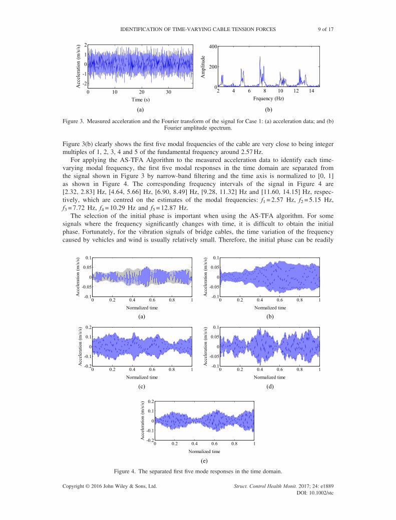
Figure 3. Measured acceleration and the Fourier transform of the signal for Case 1: (a) acceleration data; and (b)Fourier amplitude spectrum.


Figure 3(b) clearly shows the first five modal frequencies of the cable are very close to being integermultiples of 1, 2, 3, 4 and 5 of the fundamental frequency around 2.57Hz.

For applying the AS-TFA Algorithm to the measured acceleration data to identify each time-varying modal frequency, the first five modal responses in the time domain are separated fromthe signal shown in Figure 3 by narrow-band filtering and the time axis is normalized to [0, 1]as shown in Figure 4. The corresponding frequency intervals of the signal in Figure 4 are[2.32, 2.83] Hz, [4.64, 5.66] Hz, [6.90, 8.49] Hz, [9.28, 11.32] Hz and [11.60, 14.15] Hz, respec-tively, which are centred on the estimates of the modal frequencies: f1 = 2.57 Hz, f2 = 5.15 Hz,f3 = 7.72 Hz, f4 = 10.29 Hz and f5 = 12.87 Hz.

The selection of the initial phase is important when using the AS-TFA algorithm. For somesignals where the frequency significantly changes with time, it is difficult to obtain the initialphase. Fortunately, for the vibration signals of bridge cables, the time variation of the frequencycaused by vehicles and wind is usually relatively small. Therefore, the initial phase can be readily

Figure 4. The separated first five mode responses in the time domain.



estimated from the modal frequencies which are obtained by picking a modal peak in thefrequency domain

θ0 ¼ 2πnf kf

ν (28)

where n is the length of signal; fk is the kth modal frequency; f is the sampling frequency (f=200Hz in this example); and ν= [0 : 1/(n� 1) : 1]T is a normalized time axis vector. The initial phasefor the AS-TFA algorithm can be calculated using Eqn (28) for each of the first five modalfrequencies with sample length n= 7774 giving θ0 = 628.40ν, 1256.80ν, 1885.2ν, 2513.60ν and3142.00ν, respectively.

Applying the AS-TFA algorithm to each modal response in Figure 4, the identified time-frequencyresults of Case 1 are shown in Figure 5(a) for the first five time-varying modal frequencies. Forcomparison, the Hilbert–Huang transform (HHT) calculated using the Matlab Toobox developed byN. Huang et al. (http://rcada.ncu.edu.tw/research1.htm) is also employed to identify the first fivetime-varying modal frequencies, and the results are shown in Figure 5(b). Figure 5 shows that theidentified time-varying modal frequencies by AS-TFA algorithm are much smoother and more stablethan the HHT results.

Using each of these five time-varying frequencies to calculate the cable tension forces byEqn (27), the results are shown in Figure 6, where the solid lines (labelled ‘Measured’) are thecable tension forces measured by the force sensor without de-noising in the experiments, the dottedlines (labelled ‘HHT’) are the identified cable tension forces by the HHT method, and the dashedlines (labelled ‘AS-TFA’) are the identified cable tension forces by the AS-TFA method. As shownin Figure 6, the identified time-varying cable tension forces are close to the measured cable tensionforces, especially for the AS-TFA Algorithm. The calculated cable tension forces from the HHTmethod in Figure 6 are much more noisy, especially for the fourth and fifth time-varying modalfrequencies. To quantify the identification error, the relative error of the cable tension force iscalculated by

ξa ¼eFa � T

�� 2

Tk k2�100% (29)

Figure 5. Identified first five time-varying frequencies for Case 1: (a) adaptive sparse time frequency analysis; and(b) Hilbert–Huang transform.


http://rcada.ncu.edu.tw/research1.htm

Figure 6. Identified time-varying cable tension forces of Case 1 using the first five time-varying modal frequenciesfrom adaptive sparse time frequency analysis (AS-TFA) and Hilbert–Huang transform (HHT), which are shown

from (a) to (e) from the first through to the fifth modal frequency.


ξh ¼eFh � T

�� 2

Tk k2�100% (30)

where ξa and ξh are the percentage identification errors of the cable-tension forces identified

by adaptive sparse time-frequency and HHT based methods, respectively; eFa ¼eFa t1ð Þ;…; eFa tNð Þh i

and eFh ¼ eFh t1ð Þ;…; eFh tNð Þh i

are the identified cable tension force vectors

for these two methods; and T = [T(t1),…, T(tN)] is the measured cable tension force at thesampled times. The identification errors for the cable tension forces calculated using the iden-tified first to fifth time-varying modal frequencies from the AS-TFA algorithm are:ξa = 4.26%, 3.62%, 3.27%, 4.36% and 3.43%, respectively. The identification errors for thecable tension forces calculated using the identified first to fifth time-varying modal frequen-cies by using the HHT method are: ξh = 5.29%, 3.34%, 3.41%, 5.83% and 5.20%,respectively.

Figure 6 shows that the time-varying cable forces estimated using each identified modal frequencyhave some differences. We now impose the constraints between the higher-order modal frequenciesand the fundamental frequency of the cable and set the parameter K=5 and the initial phase



θ0 = 628.40ν in the AS-TFA Algorithm. The identification results obtained from AS-TFA Algorithmare shown in Figure 7, where the identified time-varying cable force for Case 1 is smooth and stable,and it has a corresponding identification error of ξa=3.34%.

4.2.2. Identification results for Case 2. For Case 2, the measured cable acceleration signal with lengthn=8630 and its Fourier amplitude spectrum within a frequency range of [2,15] Hz are shown in Figure 8.

With the same calculation procedure as used in Case 1, applying the AS-TFA Algorithm to the first fivemodal responses separated from the measured acceleration data, which are shown in Figure 8(a), leads to theidentified time-frequency results of Case 2 that are shown in Figure 9(a), which clearly shows the first fivetime-varying modal frequencies. Comparing with the identification results by using the HHTmethod, whichare shown in Figure 9(b), the adaptive sparse time frequency analysis method obviously produces much bet-ter results.

The time-varying cable tension force identification results of Case 2 are shown in Figure 10, which showsthat the time-varying cable tension force can be well identified by the adaptive sparse time-frequency anal-ysis method with small identification error compared with the HHT based results. The corresponding cabletension force identification error for both of these methods are: ξa=3.76%, 3.62%, 3.53%, 4.25%, 3.46%;and: ξh=8.84%, 8.30%, 5.69%, 5.94%, 7.15%, respectively. The identification results from combining thefirst five time-varying modal frequencies are also smoother and more stable than the results identified fromeach signal frequency, as shown in Figure 11, where the identification error is 3.58%.

4.2.3. Identification results for Case 3. For the more complex scenario of Case 3, the measured cableacceleration signal length n=56999 and its Fourier amplitude spectrum within a frequency range of[2,15] Hz are shown in Figure 12.

The identified time-frequency results for Case 3 from using the adaptive sparse time-frequency andHHT methods are shown in Figure 13. Obviously, the adaptive sparse time-frequency based results are

Figure 7. Identified time-varying cable tension force for Case 1 by combining the first five time-varying frequencies, with the identification error ξa= 3.34%. AS-TFA, adaptive sparse time frequency analysis.

Figure 8. Measured acceleration and the Fourier transform of the signal for Case 2: (a) acceleration data; and (bFourier amplitude spectrum.


-

)

Figure 9. Identified first five time-varying frequencies for Case 2: (a) adaptive sparse time frequency analysis; and(b) Hilbert–Huang transform.

Figure 10. Identified time-varying cable tension forces of Case 2 using the first five time-varying frequencies fromadaptive sparse time frequency analysis (AS-TFA) and Hilbert–Huang transform (HHT), which are shown from

(a) to (e) for the first through to the fifth modal frequency.



Figure 11. Identified time-varying cable tension force of Case 2 by combining the first five time-varying frequen-cies, with the identification error ξa= 3.58%. AS-TFA, adaptive sparse time frequency analysis.

Figure 12. Measured acceleration and the Fourier transform of the signal for Case 3: (a) acceleration data; and (bFourier amplitude spectrum.

Figure 13. Identified first five time-varying frequencies for Case 3: (a) adaptive sparse time frequency analysisand (b) Hilbert–Huang transform.



)

much smoother and more stable than the HHT based results. Using each of these five time-varying fre-quencies, the calculated time-varying cable tension forces are shown in Figure 14, which shows thatthe AS-TFA based identification results are close to the measured cable forces, with relative identifica-tion errors: ξa=3.04%, 2.96%, 2.56%, 2.50% and 2.26% for each of the five time-varying modal fre-quencies. However, the corresponding identification errors for the HHT based results are significantlylarger: ξh=5.62%, 4.23%, 5.19%, 5.36% and 5.98%, respectively. In this case, the results obtained by

;

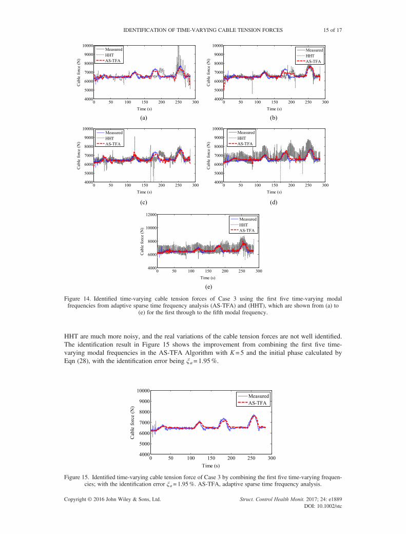
Figure 14. Identified time-varying cable tension forces of Case 3 using the first five time-varying modalfrequencies from adaptive sparse time frequency analysis (AS-TFA) and (HHT), which are shown from (a) to

(e) for the first through to the fifth modal frequency.


HHT are much more noisy, and the real variations of the cable tension forces are not well identified.The identification result in Figure 15 shows the improvement from combining the first five time-varying modal frequencies in the AS-TFA Algorithm with K=5 and the initial phase calculated byEqn (28), with the identification error being ξa=1.95%.

Figure 15. Identified time-varying cable tension force of Case 3 by combining the first five time-varying frequen-cies; with the identification error ξa= 1.95%. AS-TFA, adaptive sparse time frequency analysis.



5. CONCLUSIONS

A time-varying cable tension force identification method based on adaptive sparse time-frequencyanalysis is proposed in this paper where the first step is to estimate the time-varying modal frequenciesfrom a cable vibration signal, and the second step is to use these results to calculate the time-varyingcable tension force by flat taut string theory. Additional robustness of the method is provided byconsidering the integer ratios of the different modal frequencies to the fundamental frequency of thecable in the adaptive sparse time-frequency algorithm.

The results of cable experiments show that the time-varying modal frequencies of the cable can bewell identified by the proposed adaptive sparse time-frequency algorithm and that the time-varying ca-ble tension forces calculated from each time-varying frequency separately are close to the force sensormeasurements. A comparison of the results obtained from the HHT method and the proposed approachshow that the latter results are much more stable and have smaller identification errors. The identifiedfirst five time-varying modal frequencies from the cable experiment can be combined to produce moreaccurate and more robust results. The relative identification errors of the time-varying cable tensionforces for all three experimental scenarios are less than 5%, which is an acceptable error for structuralhealth monitoring purposes.

We expect that the procedure of looking for the sparsest decomposition among all feasible decom-positions based on a redundant time-frequency dictionary could also be achieved using a Bayesianmodel selection method. For future research, it would be interesting to develop a Bayesian methodfor sparse time-frequency analysis for the identification of time-varying cable tension forces andcompare the results with the approach proposed in this paper.

ACKNOWLEDGEMENTS

One of the authors (Yuequan Bao) acknowledges the support provided by the China Scholarship Council while hewas a Visiting Associate at the California Institute of Technology. This research was also supported by grants fromthe National Basic Research Program of China (Grant No.2013CB036305), the National Natural Science Founda-tion of China (Grant No. 51378154, 51161120359), which supported the first and fourth authors (Yuequan Baoand Hui Li). The research of Zuoqiang Shi was supported by National Natural Science Foundation of China (GrantNo. 11371220). The research of Thomas Hou and Zuoqiang Shi was also in part supported by National ScienceFoundation of USA (Grant DMS-1318377).

REFERENCES

1. Ou J, Li H. Structural health monitoring in mainland China: review and future trends. Structural Health Monitoring 2010;9(3):219–232.

2. Mufti AA. Structural health monitoring of innovative Canadian civil engineering structures. Structural Health Monitoring2002; 1(1):89–103.

3. Ko JM, Ni YQ. Technology developments in structural health monitoring of large-scale bridges. Engineering Structures2005; 27(12):1715–1725.

4. Jang S, Jo H, Cho S, Mechitov K, Rice JA, Sim SH, Jung HJ, Yun CB, Spencer BF Jr, Agha G. Structural health monitoringof a cable-stayed bridge using smart sensor technology: deployment and evaluation. Smart Structures and Systems 2010;6(5-6):439–459.

5. Kim BH, Park T. Estimation of cable tension force using the frequency-based system identification method. Journal ofSound and Vibration 2007; 304:660–676.

6. Casas JR. A combined method for measuring cable forces: the cable-stayed Alamillo Bridge, Spain. Structural EngineeringInternational 1994; 4(4):235–240.

7. Gentile C. Deflection measurement on vibrating stay cables by non-contact microwave interferometer. NDT & E Interna-tional 2010; 43(3):231–240.

8. Kim BH, Shin HY. A comparative study of the tension estimation methods for cable supported bridges. InternationalJournal of Steel Structures 2007; 7(1):77–84.

9. Ren WX, Liu HL, Chen G. Determination of cable tensions based on frequency differences. Engineering Computations2008; 25(2):172–189.

10. Russell JC, Lardner TJ. Experimental determination of frequencies and tension for elastic cables. Journal of EngineeringMechanics 1998; 124(10):1067–1072.

11. Humar JL. Dynamics of Structures. Prentice Hall: Upper Saddle River, NJ, 2000.12. Fang Z, Wang J. Practical formula for cable tension estimation by vibration method. Journal of Bridge Engineering 2012;

17:161–164.13. Sim SH, Li J, Jo H, Park JW, Cho S, Spencer BF Jr, Jung HJ. A wireless smart sensor network for automated monitoring of

cable tension. Smart Materials and Structures 2014; 23(2):025006.



14. Zui H, Shinke T, Namita YH. Practical formulas for estimation of cable tension by vibration method. ASCE Journal ofStructural Engineering 1996; 122(6):651–656.

15. Liao W, Ni Y, Zheng G. Tension force and structural parameter identification of bridge cables. Advances in StructuralEngineering 2012; 15(6):983–996.

16. Cho S, Lynch JP, Lee JJ, Yun CB. Development of an automated wireless tension force estimation system for cable-stayedbridges. Journal of Intelligent Material Systems and Structures 2010; 21(3):361–376.

17. Li H, Zhang F, Jin Y. Real-time identification of time-varying tension in stay cables by monitoring cable transversalacceleration. Structural Control Health Monitoring 2014; 21:1100–1111.

18. Yang Y, Li S, Nagarajaiah S, Li H, Zhou P. Real-time output-only identification of time-varying cable tension fromaccelerations via Complexity Pursuit. ASCE Journal of Structural Engineering 2015; 142(1): 04015083.

19. Wang LM, Wang G, Zhao Y. Application of EM stress sensors in large steel cables. In Sensing Issues in Civil StructuralHealth Monitoring, Ansari F (ed). Springer: Berlin, Germany, 2005; 145–154.

20. Sumitro S, Kurokawa S, Shimano K, Wang ML. Monitoring based maintenance utilizing actual stress sensory technology.Smart Materials and Structures 2005; 14:S68–S78.

21. Yim J, Wang ML, Shin SW, Yun CB, Jung HJ, Kim JT, Eem SH. Field application of elasto-magnetic stress sensors formonitoring of cable tension force in cable-stayed bridges. Smart Structural and Systems 2013; 12(3-4):465–482.

22. Hou TY, Shi Z. Adaptive data analysis via sparse time-frequency representation. Advances in Adaptive Data Analysis 2011;3(1&2):1–28.

23. Hou TY, Shi Z. Data-driven time-frequency analysis. Applied and Computational Harmonic Analysis 2013; 35(2):284–308.24. Hou TY, Shi Z, Tavallali P. Convergence of a data-driven time-frequency analysis method. Applied and Computational

Harmonic Analysis 2014; 37(2):235–270.25. Huang NE, Shen Z, Long SR, Wu MC, Shih HH, Zheng Q, Yen NC, Tung CC, Liu HH. The empirical mode decomposition

and the Hilbert spectrum for nonlinear and non-stationary time series analysis. Proceedings of the Royal Society of LondonA: Mathematical, Physical and Engineering Sciences 1998; 454:903–995.

26. Candes EJ. Compressive sampling. Proceedings of the International Congress of Mathematicians, Madrid, Spain, 2006:1433–1452.

27. Donoho D. Compressed sensing. IEEE Transactions on Information Theory 2006; 52(4):1289–1306.28. Baraniuk R. Compressive sensing. IEEE Signal Processing Magazine 2007; 24(4):118–121.29. Casciati F, Ubertini F. Nonlinear vibration of shallow cables with semiactive tuned mass damper. Nonlinear Dynamics 2008;

53(1-2):89–106.30. Faravelli L, Ubertini F. Nonlinear state observation for cable dynamics. Journal of Vibration and Control 2009;

15(7):1049–1077.31. Faravelli L, Fuggini C, Ubertini F. Toward a hybrid control solution for cable dynamics: theoretical prediction and experi-

mental validation. Structural Control and Health Monitoring 2010; 17(4):386–403.


identification of time-varying cable tension forces based...

Documents