1

Identification of Workstations in Earthwork Operations from Vehicle GPS Data Jiali Fu, Corresponding Author Department of Transport Science KTH Royal Institute of Technology Teknikringen 10, 10044 Stockholm, Sweden Tel: +46 8 790 8007; Email: jiali.fu@abe.kth.se Erik Jenelius Department of Transport Science KTH Royal Institute of Technology Teknikringen 10, 10044 Stockholm, Sweden Tel: +46 8 7908032; Email: erik.jenelius@abe.kth.se Haris N. Koutsopoulos Department of Civil and Environmental Engineering Northeastern University 360 Huntington Avenue, Boston, USA Department of Transport Science KTH Royal Institute of Technology Teknikringen 10, 10044 Stockholm, Sweden Tel: +46 8 7909746; Email: h.koutsopoulos@neu.edu

Preprint of paper accepted for publication in Automation in Construction

Abstract The paper proposes a methodology for the identification of workstations in earthwork operations based on GPS traces from construction vehicles. The model incorporates relevant information extracted from the GPS data to infer locations of different workstations as probability distributions over the environment. Monitoring of workstation locations may support map inference for generating and continuously updating the layout and road network topology of the construction environment. A case study is conducted at a complex earthwork site in Sweden. The workstation identification methodology is used to infer the locations of loading stations based on vehicle speeds and interactions between vehicles, and the locations of dumping stations based on vehicle turning patterns. The results show that the proposed method is able to identify workstations in the earthwork environment efficiently and in sufficient detail. Keywords: Earthwork operations, Global Positioning System (GPS), location detection, probabilistic model, kernel density estimation 1. Introduction Heavy construction refers to large-scale projects such as construction of infrastructure (highways, streets and railways), flood control, and mining and quarry operations.

2

Earthwork, in particular, is the processing and moving of large quantities of soil from the earth’s surface, and is an important part of the early stages of heavy construction projects. Earthwork operations involve processes such as excavating, hauling, dumping, crushing and compacting soil. Activities are typically equipment-driven, and most frequently include excavators, loaders, compactors and hauling trucks. Earthwork environments are highly dynamic by nature. Especially during the early stages of projects, the layout of the construction site and the road geometry change continuously. As the operation proceeds, the construction site expands and workstations move further away from each other, driving times between workstations become longer and the loading units may stand idle while waiting for hauling units. The performance of the fleet thus declines, including productivity reduction, increased cost and reduced utilization of certain types of equipment [1]. In such situations, it is crucial that management take actions and adjust the operations so that performance does not deviate much from the plan. Such actions may include increasing the number of hauling vehicles or changing to hauling vehicles with higher capacities. Even if there is no possibility to change the fleet composition, the negative effects due to site expansion can be reduced by adjusting operating methods. Such alterative operating methods may include, e.g., not loading the hauling trucks to their full capacity and thus reducing the driving time, fuel consumption of hauling units, and idle time for loading units. The project management thus needs to regularly update the map of the environment in order to accurately plan and monitor the work process. It is hence important to be able to track the number and locations of significant areas, including loading and dumping workstations, haulage roads, road intersections etc., and the network of transport paths between them [2]. The rate of change of workstations is high at construction sites of moderate scales. In large construction sites, the workstations are more significant and the locations are most likely known in the designing phase of the projects. In any case, the locations of certain types of workstations, such as loading stations, are moving gradually further away as the projects progress. It is thus necessary to follow the development of projects and make appropriate adjustment in the operations so that the performance is not much affected. Traditionally, mapping of the site layout requires manual data collection, which can be time and resource consuming [3]. Some large-scale heavy construction operations even engage helicopters with advanced laser scanning technology to take aerial photographs with 3-dimensional geographical information of the site at regular intervals. This method can help managers to accurately deduce the site layout and road geometry at a high accuracy, but is expensive to repeat frequently. The recent spread of mobile GPS devices opens up the possibility for easy collection of location data, and facilitates the development of a variety of location-aware applications. For example, information from vehicles’ movement data is already finding applications in areas such as city planning [4], real-time traffic management [5], and fleet management [6]. GPS devices have become standard equipment for construction vehicles in recent years. The paper proposes a methodology for inferring the locations of distinct types of workstations in earthwork operations from vehicle GPS data logs. The proposed method makes use of the “free” GPS trace data from daily operations, and does not require other

3

signals from vehicle Controller Area Network (CAN) buses or prior knowledge of the operating environment. Compared to manually identifying workstations from aerial photographs, the proposed approach does not require input or experience in the construction field on the part of the users. Thus, the approach may identify the locations of critical work stations at a fraction of the cost of traditional approaches. Theidentification of workstation locations may be used as part of a wider mapinference framework for generating and updating the layout and road networktopologyoftheconstructionenvironmentasitevolvesovertime.Theproblemisimportantinlightoftheuseofsimulation‐basedoptimizationtoolsformodellingthe complex characteristics of earthworkoperations, and for allocating themostsuitablevehiclefleetandoperatingmethods[7]. The methodology employs various characteristics in vehicle movements and interactions during earthwork operations to generate probability distributions over the site geometry for the locations of different workstations. Specific models are developed in order to infer the locations of loading stations, where excavated material is loaded onto hauling trucks, based on interactions between loading and hauling vehicles, and the locations of dumping stations based on hauling vehicles’ turning movements. Furthermore, a clustering method is used to calculate the number of distinct workstations of each type. The methodology is applied in a case study at an earthwork site in Sweden. GPS data are collected from a group of construction vehicles working together, and processed using the proposed methodology to extract locations of various workstations. The experimental results indicate that the proposed method is capable to infer the most important workstations in earthwork operations. The remainder of the paper is structured as follows. A review of related prior work is given in Section 2. Section 3 presents the probabilistic framework for the identification of different workstations. The case study is described in Section 4, with results discussed in Section 5. Section 6 concludes the paper and identifies future research directions. 2. Related Work A number of studies have presented methods for inferring significant locations (i.e., locations that plays a significant role in the activities of the agent) from GPS traces, focusing primarily on road traffic and pedestrian movement. One proposed method automatically clusters places where the user spends a minimum pre-defined amount of time into significant locations, and uses a Markov model to predict the agent’s movements [8]. Other approaches include spatio-temporal clustering to identify stops and movements in trajectories based on the speed profile [9], and a stay extraction algorithm using pre-defined scale parameters such as a maximum distance from or a minimum duration at a location [10]. Other studies use clustering and fixed-threshold-based criteria to identify significant locations [11, 12, 13]. A drawback of methods based on fixed thresholds is that inference is sensitive to the choice of threshold parameters. Furthermore, suitable thresholds can vary significantly depending on application context and GPS data source. In practice, there is no standard

4

threshold that leads to a satisfactory detection of all significant places. Thus, success of the approach depends heavily on the design decisions as well as the quality and frequency of the GPS data. Machine learning methods have also been employed for the inference of significant places in various applications, mainly for the analysis of individuals’ travel and activity patterns. The proposed methods include a Gaussian mixture model for inferring agent’s significant locations from GPS data [14], a dynamic Bayesian network model for inferring transport modes between significant places [15], and a conditional random fields model for inferring a person’s activities and significant places [16]. Based on GPS traces, the latter model first segments an agent’s day into activities of work, visits or travel, and then identifies significant places such as workplace, home, or restaurant. Other approaches include a probabilistic place extraction algorithm based on the density of data points [17], where high-density regions are ranked by importance using a density scoring metric. Similarly, kernel density estimation has been applied to GPS traces to create a continuous density surface from which local maxima are retained as stop locations [18]. In contrast to the settings of the studies above, earthwork environments are highly unstructured and dynamic, and vehicles do not always follow predictable routines. Thus, it is necessary to tackle the location identification problem in these applications in a different manner [19]. Vehicle speed, for example, may provide meaningful information in the case of off-road construction environments. If a vehicle is moving very slowly in a particular area, it may indicate that the vehicle is performing an activity (loading, unloading, queuing or yielding). In the context of safety, one approach is to identify activity locations with potential interactions between vehicles and risk of accidents uses a probabilistic model based on vehicle speed profiles [19]. Examples from an open pit mine show that the algorithm detected important locations successfully. The detected locations are forwarded to a collision avoidance system for mining operations, which provides warnings and driving assistance to vehicle operators [20]. This method detects important locations from a safety point of view, but is not designed for identifying the contextual information of a construction environment. With the same reasoning, a speed-based method is presented in [21] for automatic work zone detection for trucks, and suggested using GPS data and the concept of work zones for the extraction and analysis of cycle time information. However, the proposed zone detection method is not able to identify the type of work zones and manual input is therefore required. In contrast to [19], an important motivation for this study is to use the inferred up-to-date layout as input to a simulation-based optimization framework for optimization of various aspects of site operations, such as vehicle fleet combination and alternative operating methods [7]. For this application, it is essential to have accurate information on the locations of specific workstations rather than general significant places. In the proposed method, more complex activity characteristics than vehicles’ speed profiles, such as interactions between difference vehicle types and vehicle turning movements, are employed for the inference of different types of workstations. Information regarding the movements and interactions between construction vehicles is extracted from synchronized GPS data from multiple vehicles.

5

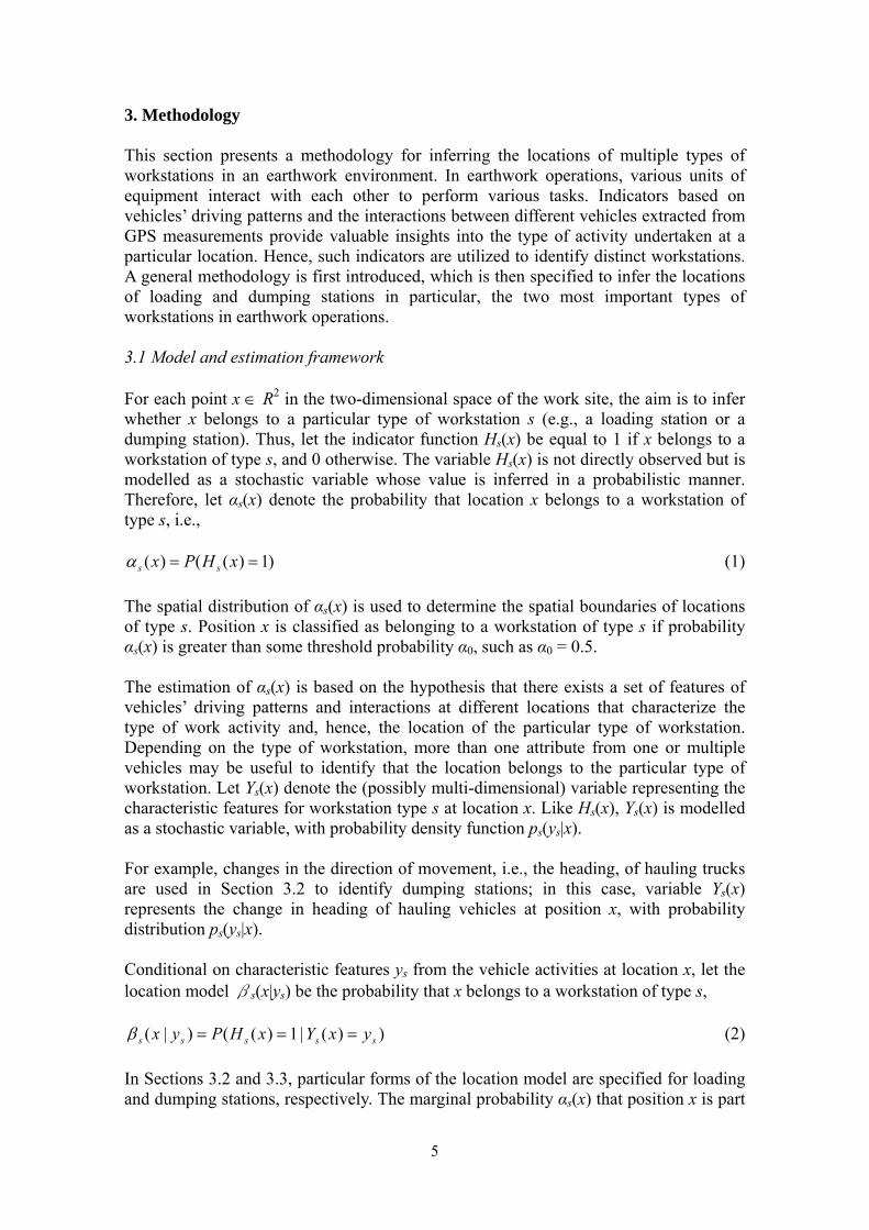
3. Methodology This section presents a methodology for inferring the locations of multiple types of workstations in an earthwork environment. In earthwork operations, various units of equipment interact with each other to perform various tasks. Indicators based on vehicles’ driving patterns and the interactions between different vehicles extracted from GPS measurements provide valuable insights into the type of activity undertaken at a particular location. Hence, such indicators are utilized to identify distinct workstations. A general methodology is first introduced, which is then specified to infer the locations of loading and dumping stations in particular, the two most important types of workstations in earthwork operations. 3.1 Model and estimation framework For each point x R2 in the two-dimensional space of the work site, the aim is to infer whether x belongs to a particular type of workstation s (e.g., a loading station or a dumping station). Thus, let the indicator function Hs(x) be equal to 1 if x belongs to a workstation of type s, and 0 otherwise. The variable Hs(x) is not directly observed but is modelled as a stochastic variable whose value is inferred in a probabilistic manner. Therefore, let αs(x) denote the probability that location x belongs to a workstation of type s, i.e.,

)1)(()( xHPx ss (1)

The spatial distribution of αs(x) is used to determine the spatial boundaries of locations of type s. Position x is classified as belonging to a workstation of type s if probability αs(x) is greater than some threshold probability α0, such as α0 = 0.5. The estimation of αs(x) is based on the hypothesis that there exists a set of features of vehicles’ driving patterns and interactions at different locations that characterize the type of work activity and, hence, the location of the particular type of workstation. Depending on the type of workstation, more than one attribute from one or multiple vehicles may be useful to identify that the location belongs to the particular type of workstation. Let Ys(x) denote the (possibly multi-dimensional) variable representing the characteristic features for workstation type s at location x. Like Hs(x), Ys(x) is modelled as a stochastic variable, with probability density function ps(ys|x). For example, changes in the direction of movement, i.e., the heading, of hauling trucks are used in Section 3.2 to identify dumping stations; in this case, variable Ys(x) represents the change in heading of hauling vehicles at position x, with probability distribution ps(ys|x). Conditional on characteristic features ys from the vehicle activities at location x, let the location model βs(x|ys) be the probability that x belongs to a workstation of type s,

))(|1)(()|( sssss yxYxHPyx (2)

In Sections 3.2 and 3.3, particular forms of the location model are specified for loading and dumping stations, respectively. The marginal probability αs(x) that position x is part

6

of a workstation of type s is obtained by integrating βs(x|ys) across all possible values of ys, each weighted by the probability density ps(ys|x) of observing ys at x,

ssssss dyxypyxx )|()|()( (3)

The probability density ps(ys|x) is estimated based on vehicle GPS traces from the work site. A GPS trace includes GPS probes with frequency 1/Δt, where each probe includes a timestamp t and the corresponding longitude and latitude coordinates, xt. In general, synchronized GPS traces from multiple vehicles may be used to infer ps(ys|x). Thus, let

TtstMtts yxxZ 1

1 ,,..., be a data set containing synchronized, sequential position

measurements 1tx ,…, M

tx from M vehicles over time period T, and values sty of the

characteristic variable derived from the GPS traces for identifying workstations of type s. The conditional probability density ps(ys|x) is expressed as ps(ys|x) = ps(x, ys)/p(x), where ps(x, ys) is the joint probability density of simultaneously observing characteristic features ys and position x from the GPS traces. p(x) is the marginal probability density of observing the vehicle(s) generating the GPS traces simultaneously at position x. The marginal probability αs(x) is thus obtained as

ssssss dyyxpyxxp

x ),()|()(

1)( (4)

Kernel density estimation [22] is used to estimate the probability density functions ps(x, ys) and p(x) across the work site over time period T. That is,

T

tst

Mtts yyxxxx

Tyxp

1

11 ,,...,

1),( , (5)

T

t

Mtts xxxx

Txp

1

12 ,...,

1)( , (6)

where κ1 and κ2 are kernel density functions for estimating ps(x, ys) and p(x), respectively. The Gaussian kernel is used here due to its convenient mathematical properties, although the choice of the kernel function is not critical for the accuracy of the estimator. In the following section, the general methodology is specified for the inference of loading and dumping stations, respectively. 3.2. Identification of loading stations For earthwork with loading and hauling vehicles, the loading vehicles repeat cycles of driving towards the material pile to fill the bucket (phase 1), reversing (phase 2) and then driving forward (phase 3) to empty the bucket (phase 4) on the container of the receiving truck (Figure 1). These driving patterns and interactions are common to the majority of situations [23], [24]. While waiting for an empty truck to arrive to start the

7

next loading cycle, the loader may clean the working site, preparing it for the next loading cycle. Work cycles for hauling trucks consist of driving between the loading station for loading and the dumping station for emptying their load. During loading, the receiving truck remains still and the loading unit keeps driving forward and reversing to empty and fill its bucket.

Figure 1: Loading process.

It is hypothesized that, under normal working conditions, the presence of both loading and hauling vehicles at the same location while driving at low speeds or standing still is a suitable indicator for identifying loading stations. Let VLU(x) and VHU(x) be stochastic variables denoting the speed at location x of the loading and the hauling vehicles, respectively. Then the conditional probability of position x being part of a loading station given the simultaneous speeds of the loading unit vLU and hauling unit vHU is

))(,)(|1)((),|( HUHULULUloading

HULUloading vxVvxVxHPvvx (7)

In the following, βloading(x|vLU, vHU) is modelled as a binary variable, equal to 1 if the speeds of the two units are lower than thresholds LU

maxv and HUmaxv , respectively, and 0

otherwise. The speed thresholds LUmaxv and HU

maxv are model parameters that are used to

distinguish between the lower speed of the loading activity and the relatively higher speeds of hauling vehicles. Thus,

HUmax

HU

LUmax

LUHULU

loading ),|(v

vI

v

vIvvx , (8)

where I(x) is a step function equal to 1 for x≤1 and 0 otherwise. In other words,

)/( LUmax

LU vvI is 1 if the speed of the loading vehicle is lower than or equals to the

maximum speed limit LUmaxv , and zero otherwise. The indicator function )/( HU

maxHU vvI for

the hauling unit is defined analogously.

8

The temporal information in the GPS data is utilized to compute the probability of detecting both loading and hauling vehicles at low speeds simultaneously at the same location. Let LU

tv denote the instantaneous speed of the loading unit at time t calculated

from the position measurements as

t

xxv

tt

t

LU1

LU

LU (9)

The speed of the hauling unit, denoted HU

tv , is defined analogously. The kernel density

estimator for the joint probability density pLU,HU(x, vLU, vHU) of both vehicles simultaneously at position x at speeds vLU and vHU over a time period T is

T

t v

t

v

t

x

t

x

t

vvxx

vvvvxxxx

T

vvxp

1HU

HUHU

LU

LULU

HU

HU

LU

LU

HULUHULU

HULUHULU,

1

),,(

(10)

where φ(x) is the standardized Gaussian distribution (i.e., with 0 mean and standard deviation 1), and LU

x , HUx , LU

v and HUv are standard deviation for the respective

measurement type (position and speed) and vehicle type (loader and hauler). The joint probability density function pLU,HU(x) of both loading and hauling units being simultaneously at location x over a time period T is similarly estimated as

HU

HU

1LU

LU

HULUHULU, 1

)(x

tT

t x

t

xx

xxxx

Txp

(11)

The marginal probability αloading(x) that position x belongs to a loading station is obtained by integrating over the latent speed variables vLU and vHU, each weighted by the conditional probability density estimated from the GPS data,

HULUHULUHULU,HULUloadingHULU,loading ),,(),|(

)(

1)( dvdvvvxpvvx

xpx (12)

Inserting the conditional loading station probability βloading(x|vLU, vHU) from (8) and the kernel density estimators of pLU,HU(x,vLU, vHU) and pLU,HU(x) from (10) and (11) into (12) yields

HU

HU

1LU

LUHULU

1HU

HUHUmax

LU

LULUmax

HU

HU

LU

LU

loading )(

x

tT

t x

tvv

T

t v

t

v

t

x

t

x

t

xxxx

vvvvxxxx

x

(13)

where Φ(x) denotes the standard Normal cumulative distribution function.

9

3.3. Identification of dumping stations Arriving at a dumping station, the fully loaded hauling truck typically first needs to make a turning movement (phase 1 in Figure 2) and reverse to the dumping spot (phase 2) in order to empty its load (phase 3) properly. The vehicle then drives away from the dumping spot (phase 4) to return to the loading station. Thus, the driving patterns of hauling trucks consist of several sharp turns determined by the geometry of the site [25]. Typically, the changes in movement direction just before/after dumping are approximately 180°.

Figure 2: Dumping process.

It is hypothesized that large heading differences in the hauling vehicles’ GPS traces can be utilized to infer the positions of dumping stations. Let ΔHU(x) denote the stochastic variable representing the change in heading of the hauling vehicle at location x, defined to be in the interval from 0° to 180°. The conditional probability of position x being part of a dumping station given heading change δHU is then

))(|1)(()|( HUHUdumping

HUdumping xxHPx (14)

Similar to the identification of loading stations in Section 3.2, an indicator variable is used to model βdumping(x|δHU), which is equal to 1 if the heading change is above some threshold δmin,

min

HUHU

dumping 1)|( Ix (15)

where I(x), as before, is equal to 1 for x≤1 and 0 otherwise. The heading θt (i.e., the direction in which a vehicle is moving) of the hauling vehicle at

10

time t is computed from the consecutive position measurements xt-1 and xt. The heading change is then obtained as δt = |θt – θt-1| if |θt – θt-1| ≤ 180°, between timestamps t and t-1 as depicted in the left figure 3. For heading differences larger than 180°, the conjugate angle is used as illustrated in the right figure, so the heading change is always within the interval [0°, 180°].

Figure 3: Definition of heading difference. Left: |θt – θt-1| ≤ 180°. Right: |θt – θt-1| > 180°.

The joint probability density pHU(x, δHU) of detecting a hauling unit at position x with heading change δHU over time period T is estimated by kernel density estimation as

HU

HUHU

1HU

HU

HUHUHUHU 1

),(

t

T

t x

t

x

xx

Txp (16)

where HU

v is the standard deviation for the heading change kernel. Similarly, the

estimated marginal probability density pHU(x) of observing a hauling unit at x over time period T is

T

t x

t

x

xx

Txp

1HU

HU

HUHU 1

)(

(17)

Following the general methodology, the marginal probability αdumping(x) that position x is a dumping station is obtained by integrating over the latent heading difference, weighted by the conditional probability density estimated from the GPS data,

HUHUHUHUdumpingHUdumping ),()|(

)(

1)( dxpx

xpx (18)

Inserting (15), (16) and (17) into (18) yields the final expression

T

t x

t

T

t

t

x

t

xx

xx

x

1HU

HU

1

HUmin

HU

HU

dumping

1

)(

(19)

11

3.4. Identification of distinct workstations The probabilistic model above infers whether a specific position of the work site belongs to a particular type of workstation. A clustering method is designed to add information regarding how many distinct workstations of each type exist at the site as well as the centre point of each workstation. The clustering method resembles the k-means clustering method [26], and partitions data points into mutually exclusive groups according to their GPS coordinates. In the first step, the probabilistic inference method is applied to all GPS trace points in the data set to estimate the probability of belonging to each type of workstation. GPS trace points with probability higher than the significance threshold 0 are selected and used in the next step. Subsequently, the clustering method groups the selected GPS points based on their coordinates and determines the optimal number of workstations of each type. The algorithm starts by assigning the GPS points to a small number of clusters, and then computes the centroid of each cluster as the average position of all its members. The sum of distances between the centroid and all its members is calculated. The clustering algorithm then increments the number of clusters gradually and repeats the assignment of the GPS points to clusters. The algorithm stops when the change in the sum of distances between cluster centroids and their members from the previous iteration is sufficiently small. 4. Case Study The proposed method is applied in a case study for a large quarry site located north of Stockholm, Sweden, producing gravel, aggregate, and sand. There are around 20 heavy vehicles including wheel loaders, excavators and dump trucks working at the site. Three GPS Garmin GPSmap 62 receivers are used to collect GPS traces from one wheel loader and two hauling trucks collaborating to carry out load-and-haul tasks. The GPS loggers record latitude, longitude, altitude as well as the date and time at a frequency of one measurement per second. The GPS devices have the horizontal accuracy of less than 10 meters with 95% confidence under typical use [27]. Data are collected over a four-hour period during one workday and contain approximately 14,000 trace points from each vehicle. The GPS data are processed without prior knowledge about the underlying work environment. The accuracy of the resulting locations of workstations is validated through observation at the studied construction site and confirmed by the site manager. The load-and-haul operation covers an area over two square kilometres, and the loader and the two hauling trucks travel in total approximately 20, 39 and 37 km, respectively, over the four-hour period. Figure 4 shows the GPS traces for all three vehicles (coordinates are left out for confidentiality reasons). The GPS trace points with speed lower than the speed threshold vmax for each vehicle type are shown in red in Figure 4 and the other trace points are in blue. Due to the characteristics of the operation, the low speed threshold is set to 10 km/h and 5 km/h for loading and hauling vehicles, respectively. The five stations indicated with circles are loading stations 1 and 2, the parking lot, the dumping station, and loading station 3, respectively.

12

In order to apply the kernel density estimation of the attributes used to infer loading and dumping station locations, the geometry of the work site is discretized into grids with equal spacing of 2·10-5 degrees in GPS coordinates in both dimensions (corresponding to a distance of approximately 1.3 meters between two adjacent grid points). To avoid numerical problems due to limited machine precision, the kernel probability densities are truncated to zero at positions beyond 2 meters from the nearest observed GPS position. Table 1 summarizes the various parameters used in the study.

Figure 4: GPS traces with low speed marked in red.

Table 1: Parameter values

Parameter Value Unit LUmaxv 10 km/h

HUmaxv 5 km/h

δmin 120 degrees

LUx , HU

x 10 meter

LUv , HU

v 5 km/h

45 degrees

5. Results 5.1 Identification of significant locations

Longitude

Lat

itud

e

Parking

DumpingStation

LoadingStation 1

LoadingStation 2

LoadingStation 3

13

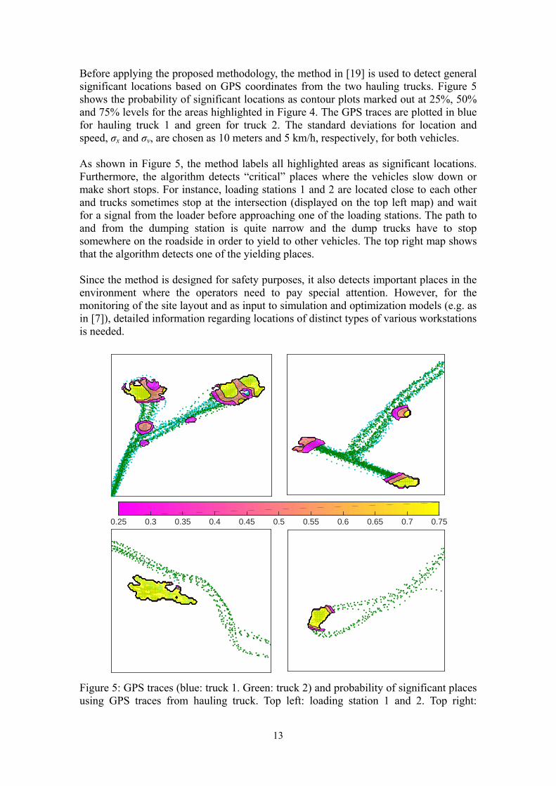
Before applying the proposed methodology, the method in [19] is used to detect general significant locations based on GPS coordinates from the two hauling trucks. Figure 5 shows the probability of significant locations as contour plots marked out at 25%, 50% and 75% levels for the areas highlighted in Figure 4. The GPS traces are plotted in blue for hauling truck 1 and green for truck 2. The standard deviations for location and speed, σx and σv, are chosen as 10 meters and 5 km/h, respectively, for both vehicles. As shown in Figure 5, the method labels all highlighted areas as significant locations. Furthermore, the algorithm detects “critical” places where the vehicles slow down or make short stops. For instance, loading stations 1 and 2 are located close to each other and trucks sometimes stop at the intersection (displayed on the top left map) and wait for a signal from the loader before approaching one of the loading stations. The path to and from the dumping station is quite narrow and the dump trucks have to stop somewhere on the roadside in order to yield to other vehicles. The top right map shows that the algorithm detects one of the yielding places. Since the method is designed for safety purposes, it also detects important places in the environment where the operators need to pay special attention. However, for the monitoring of the site layout and as input to simulation and optimization models (e.g. as in [7]), detailed information regarding locations of distinct types of various workstations is needed.

Figure 5: GPS traces (blue: truck 1. Green: truck 2) and probability of significant places using GPS traces from hauling truck. Top left: loading station 1 and 2. Top right:

0.25 0.3 0.35 0.4 0.45 0.5 0.55 0.6 0.65 0.7 0.75

14

dumping station. Bottom left: parking. Bottom right: loading station 3.

Figure 6, top diagram, shows the speeds of the loader and truck 1 during two loading cycles, as well as the distance between the two vehicles. During the loading process, the loader and the truck stand close to each other and the distance between the vehicles (black dash-dot line in the top diagram) is small. The receiving truck stands still and the speed (blue dotted line) is low. The loader repeatedly reverses and drives forward to fill its bucket and empty the content into the truck. Thus, the speed of the loader varies (shown as red solid line) rapidly and has the shape of “spikes” in the diagram. Figure 6, bottom diagram, shows the speed and heading difference of truck 1 during the same time period, and two dumping cycles are indicated. It is observed that the heading differences during dumping are large, but also during loading because of vehicle driving patterns and to some extent GPS noise. As described in Section 3.3 the heading at time t is estimated from the position measurements xt-1 and xt. Thus, the estimation of heading difference can be sensitive to GPS noise when the sequential measurements are “jumping” around at the same region.

Figure 6: Top: vehicle speed, inter-vehicle distance between loader and truck 1. Bottom: vehicle speed and heading difference of truck 1.

09:5

0:00

09:5

5:00

10:0

0:00

10:0

5:00

Sp

eed

(km

/h)

0

5

10

15

20

25

30

35

40

45

Dis

tan

ce (

m)

0

80

160

240

320

400

480

560

640

720

Loader speedTruck 1 speedDistance between loader and truck 1

09:5

0:00

09:5

5:00

10:0

0:00

10:0

5:00

Sp

ee

d (

km/h

)

0

5

10

15

20

25

30

35

40

45

50

Hea

din

g d

iffe

ren

ce (

deg

ree)

0

18

36

54

72

90

108

126

144

162

180

Truck 1 speedTruck 1 heading difference

Loading Loading

Dumping Dumping

15

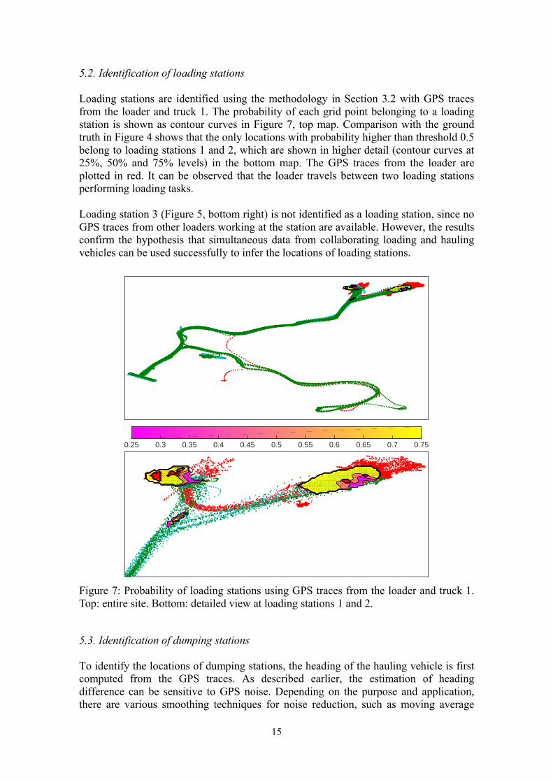
5.2. Identification of loading stations Loading stations are identified using the methodology in Section 3.2 with GPS traces from the loader and truck 1. The probability of each grid point belonging to a loading station is shown as contour curves in Figure 7, top map. Comparison with the ground truth in Figure 4 shows that the only locations with probability higher than threshold 0.5 belong to loading stations 1 and 2, which are shown in higher detail (contour curves at 25%, 50% and 75% levels) in the bottom map. The GPS traces from the loader are plotted in red. It can be observed that the loader travels between two loading stations performing loading tasks. Loading station 3 (Figure 5, bottom right) is not identified as a loading station, since no GPS traces from other loaders working at the station are available. However, the results confirm the hypothesis that simultaneous data from collaborating loading and hauling vehicles can be used successfully to infer the locations of loading stations.

Figure 7: Probability of loading stations using GPS traces from the loader and truck 1. Top: entire site. Bottom: detailed view at loading stations 1 and 2.

5.3. Identification of dumping stations To identify the locations of dumping stations, the heading of the hauling vehicle is first computed from the GPS traces. As described earlier, the estimation of heading difference can be sensitive to GPS noise. Depending on the purpose and application, there are various smoothing techniques for noise reduction, such as moving average

0.25 0.3 0.35 0.4 0.45 0.5 0.55 0.6 0.65 0.7 0.75

16

smoothing and other filtering methods [28]. In this study, the frequency of the GPS points is down sampled from 1 Hz to 0.1 Hz, i.e. one sample every 10 GPS measurements. This is a commonly employed noise-reduction method with high-resolution signals. Since the trucks travel at low speeds when changing driving directions, no valuable information is lost. Dumping stations are identified using the methodology in Section 3.3 with the down-sampled GPS traces from the hauling vehicles. The probability of each grid point being part of a dumping station is shown as contour curves in Figure 8. Only one location, the actual dumping station, over the entire working area is identified with probability above 0.5, as shown at higher detail (contour curves at 25% and 50% levels) in the bottom diagram. The highest probability of dumping station in the area is 73.74%. Due to vehicle driving patterns, heading differences are also high at the loading stations (Figure 6, bottom). However, the probability of being a dumping station according to the method in Section 3.3 in the loading area is low (less than 30%). This is because the loading process is normally spread out all over the loading zone, in contrast to the dumping procedure, which is concentrated to a particular spot. Thus, the results indicate that the method of using heading difference to identify dumping stations works well.

Figure 8: Probability of dumping stations using GPS traces from hauling vehicles. Top: entire site. Bottom: detailed view on the dumping station.

5.4. Identification of distinct workstations The clustering method described in Section 3.3. is used to identify distinct workstations

0.25 0.3 0.35 0.4 0.45 0.5

17

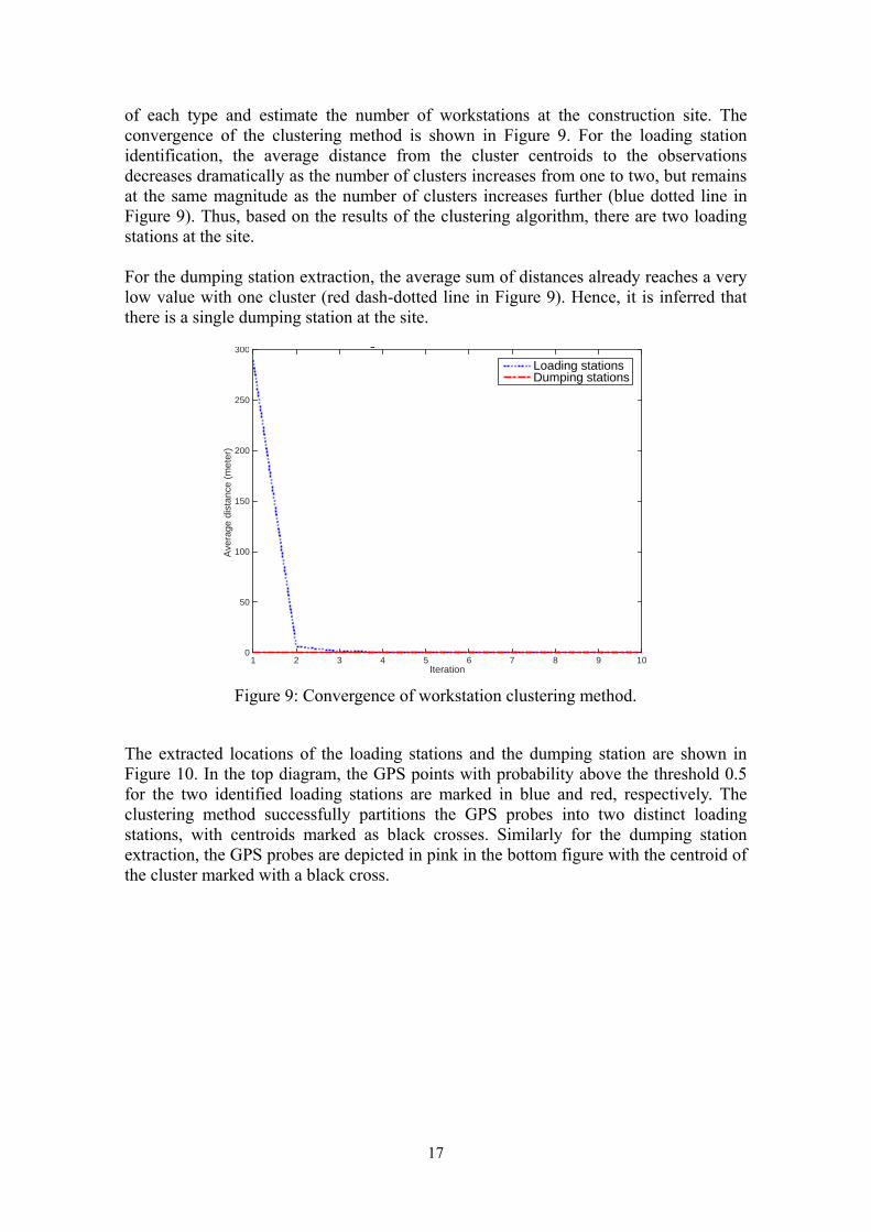
of each type and estimate the number of workstations at the construction site. The convergence of the clustering method is shown in Figure 9. For the loading station identification, the average distance from the cluster centroids to the observations decreases dramatically as the number of clusters increases from one to two, but remains at the same magnitude as the number of clusters increases further (blue dotted line in Figure 9). Thus, based on the results of the clustering algorithm, there are two loading stations at the site. For the dumping station extraction, the average sum of distances already reaches a very low value with one cluster (red dash-dotted line in Figure 9). Hence, it is inferred that there is a single dumping station at the site.

Figure 9: Convergence of workstation clustering method.

The extracted locations of the loading stations and the dumping station are shown in Figure 10. In the top diagram, the GPS points with probability above the threshold 0.5 for the two identified loading stations are marked in blue and red, respectively. The clustering method successfully partitions the GPS probes into two distinct loading stations, with centroids marked as black crosses. Similarly for the dumping station extraction, the GPS probes are depicted in pink in the bottom figure with the centroid of the cluster marked with a black cross.

Iteration1 2 3 4 5 6 7 8 9 10

Ave

rage

dis

tance

(m

ete

r)

0

50

100

150

200

250

300g

Loading stationsDumping stations

18

Figure 10: Extracted spatial centroid of workstations and GPS probes located inside. Top: extracted loading stations with GPS probes marked in red and blue for distinct stations. Bottom: dumping station with GPS probes marked in pink. Black cross: centroid of each workstation.

5.5. Sensitivity analysis Different parameter settings and sampling resolutions are tested to evaluate the sensitivity of the performance of the proposed methodology to the various thresholds. The results are summarized in Figure 11. The minimum speed thresholds for both loading and hauling units in the inference of loading stations are increased by 100% to LU

maxv = 20 and LUmaxv = 10 km/h, respectively.

The resulting probability of loading stations with higher speed thresholds is shown as contour curves at 25%, 50% and 75% levels in the top diagram. It can be observed that the probability contour is almost identical to the result with the baseline parameter setting (Figure 7). Further, the inference method of dumping stations is tested using δmin = 100° compared to 120° in the baseline setting. As shown in the middle diagram the actual dumping station is correctly identified as the only dumping station, similar to the results in the baseline setting (Figure 8). Thus, it is confirmed that the location inference methods for both loading and dumping stations perform well and are not particularly

19

sensitive to the choice of parameter values. Finally, the effect of different GPS sampling frequencies in the identification of dumping stations is examined by adjusting the resolution of the GPS data to 0.2 Hz (one sample every 5 seconds) from 0.1 Hz. It is observed in the bottom figure that the size of the significant area identified as dumping station is reduced compared to the baseline results shown in Figure 8, bottom. This result indicates that calculation of the heading difference is somewhat sensitive to the frequency of the GPS measurements, which in turn influences the performance of the inference method for dumping stations.

Figure 11: Results of sensitivity analysis. Top: Probability of loading stations with increased minimum speed threshold. Middle: probability of dumping stations using reduced heading difference threshold. Bottom: probability of dumping stations using increased sampling frequency. 6. Conclusion and Discussion Earthwork sites expand in size and change geometry over time. The paper proposed a generative model to automatically infer the locations of various types of workstations based on GPS traces from vehicles. Generally applicable characteristics of construction operations involving one or multiple vehicles are employed to infer different types of workstations. The proposed model infers the locations of various workstations as continuous probability functions over the site geometry, and provides a clear

0.25 0.3 0.35 0.4 0.45 0.5 0.55 0.6 0.65 0.7 0.75

20

interpretation of the results associated with uncertainties. The methodology does not rely on pre-defined thresholds regarding the time spent at workstations or a fixed number of workstations. Compared to the commonly employed methods in construction engineering using manual collection or scanning techniques, the approach is fully automated and consumes considerably less time and resources. The proposed methodology was evaluated in a case study with GPS data collected from three construction vehicles collaborating to carry out tasks at a quarry site. The GPS data were processed without prior knowledge about the underlying work environment. The accuracy of the resulting locations of workstations is validated through observation at the studied construction site and confirmed by the site manager. The results suggest that the proposed algorithm is capable of detecting important workstations at the studied earthwork site. For a group of construction vehicles collaborating on carrying out earthwork, the method is able to extract the locations of important workstations using GPS data from loading units and an arbitrary hauling vehicle. In the case of earthworks with one loading unit as in the case study, GPS data from the loading unit and one of the trucks are required. For earthworks with multiple loading units, it is necessary to have GPS data from all loading units in order to detect all loading stations. It is common in earthworks for each loading unit to operate at workstations relatively close to each other and hauling units to serve all loading units in the operation. Hence, the cost associated with this approach consists mainly of the cost of the GPS devices, which are currently the standard configuration for construction vehicles. In conclusion, the proposed workstation identification method is both time and cost efficient, and it is hence appropriate for extracting and updating the locations of important workstations in construction environment. The case study demonstrated the applicability of the proposed method in typical earthwork situations. In practice, due to various reasons such as internal traffic and other disturbances, the operations are not always performed as smooth as planned. However, the proposed method infers the locations as probability density function which means that the probability of a point x is a certain type of workstation is low if the event is an exceptional situation. As demonstrated in the dumping station extraction case, the hauling vehicles make sharp turns at the loading stations in order to come to the right position relatively to the loader and the heading differences of hauling vehicles (which is used to identify dumping stations) here are thus also high. Due to the reason that the loading process is spread out in the entire loading stations, the resulting probability for dumping stations at these areas is low (less than 30%). In this manner, the unusual situations yield low probability for significant workstations and therefore the proposed method is capable to handle the exceptional cases in the operations. The work opens up several interesting directions for future research. The general methodology can be extended to other types of construction environments and workstations. Further, the methodology only makes use of GPS position measurements. In addition to the location data from GPS devices, a large amount of data is increasingly becoming available from other sources such as the vehicle’s CAN buses and other on-board sensors. The data may be integrated with the GPS measurements to extract more useful representations of the construction environment and operation to achieve more efficient earthwork operations. Combination of multiple data sources can also increase

21

the certainty of the extracted information. The detection of workstations can be used as part of a more extensive map inference method to build a map of the underlying construction environment, which contains the locations of various workstations as well as the road network. The digitalized map may be continuously updated using GPS and other data collected from daily operations to capture the changes in the construction environment. Furthermore, autonomous construction equipment and construction plant control are promising developments in the industry [29]-[31]. An automatically updated digital map of site geometry will facilitate the forthcoming development. Acknowledgement This research was financially supported by the Swedish Government Agency for Innovation Systems (Vinnova). The authors would like to express their gratitude to the industry collaborator, Volvo Construction Equipment, for their support and providing access to job sites and project data. We would also like to thank the project management and equipment operators at Skanska for their help with obtaining the data used in the paper. Finally, we would like to thank two anonymous reviewers for their helpful comments and suggestions. References 1. Navon, R. (2005). Automated project performance control of construction

projects. Automation in Construction, 14(4), 467-476. DOI: https://doi.org/10.1016/j.autcon.2004.09.006.

2. Halpin, D. W., & Riggs, L. S. (1992). Planning and analysis of construction operations. John Wiley & Sons.

3. Davidson, I. N., & Skibniewski, M. J. (1995). Simulation of automated data collection in buildings. Journal of computing in civil engineering, 9(1), 9-20. DOI: http://dx.doi.org/10.1061/(ASCE)0887-3801(1995)9:1(9).

4. Castro, P. S., Zhang, D., & Li, S. (2012). Urban traffic modelling and prediction using large scale taxi GPS traces. In International Conference on Pervasive Computing (pp. 57-72). Springer Berlin Heidelberg. DOI: http://10.1007/978-3-642-31205-2_4.

5. Jenelius, E., & Koutsopoulos, H. N. (2013). Travel time estimation for urban road networks using low frequency probe vehicle data. In Transportation Research Part B: Methodological, 53, 64-81. DOI: http://doi.org/10.1016/j.trb.2013.03.008.

6. Thong, S. T. S., Han, C. T., & Rahman, T. A. (2007). Intelligent fleet management system with concurrent GPS & GSM real-time positioning technology. In the 7th International Conference on ITS Telecommunications (pp. 1-6). IEEE. DOI: 10.1109/ITST.2007.4295849.

7. Fu, J., Jenelius E., & Koutsopoulos H. N. (2013). Optimal fleet selection for earthmoving operations. In the 7th International Structural Engineering and Construction Conference, (pp. 1261-1266).

8. Ashbrook, D., & Starner, T. (2003). Using GPS to learn significant locations and predict movement across multiple users. In Personal and Ubiquitous Computing, 7(5), 275-286. DOI: 10.1007/s00779-003-0240-0.

9. Palma, A. T., Bogorny, V., Kuijpers, B., & Alvares, L. O. (2008). A clustering-

22

based approach for discovering interesting places in trajectories. In 2008 ACM Symposium on Applied Computing (pp. 863-868). ACM. DOI: 10.1145/1363686.1363886.

10. Hariharan, R., & Toyama, K. (2004, October). Project Lachesis: parsing and modeling location histories. In International Conference on Geographic Information Science (pp. 106-124). Springer Berlin Heidelberg. DOI: 10.1007/978-3-540-30231-5_8.

11. Kang, J. H., Welbourne, W., Stewart, B., & Borriello, G. (2004). Extracting places from traces of locations. In the 2nd ACM International Workshop on Wireless Mobile Applications and Services on WLAN Hotspots (pp. 110-118). ACM. DOI: 10.1145/1024733.1024748.

12. Alvares, L. O., Bogorny, V., Kuijpers, B., de Macedo, J. A. F., Moelans, B., & Vaisman, A. (2007). A model for enriching trajectories with semantic geographical information. In the 15th Annual ACM International Symposium on Advances in Geographic Information Systems (p. 22). ACM. DOI: 10.1145/1341012.1341041.

13. Zhou, C., Frankowski, D., Ludford, P., Shekhar, S., & Terveen, L. (2007). Discovering personally meaningful places: An interactive clustering approach. ACM Transactions on Information Systems (TOIS), 25(3), 12. DOI: 10.1145/1247715.1247718.

14. Zhang, K., Li, H., Torkkola, K., & Gardner, M. (2007). Adaptive learning of semantic locations and routes. In the 1st International Conference on Autonomic Computing and Communication Systems (p. 3).

15. Liao, L., Patterson, D. J., Fox, D., & Kautz, H. (2007). Learning and inferring transportation routines. In Artificial Intelligence, 171(5), 311-331. DOI: https://doi.org/10.1016/j.artint.2007.01.006.

16. Liao, L., Fox, D., & Kautz, H. (2007). Extracting places and activities from gps traces using hierarchical conditional random fields. In International Journal of Robotics Research, 26(1), 119-134. DOI: https://doi.org/10.1177/0278364907073775.

17. Kami, N., Enomoto, N., Baba, T., & Yoshikawa, T. (2010). Algorithm for detecting significant locations from raw GPS data. In International Conference on Discovery Science (pp. 221-235). Springer Berlin Heidelberg. DOI: 10.1007/978-3-642.16184-1_16.

18. Thierry, B., Chaix, B., & Kestens, Y. (2013). Detecting activity locations from raw GPS data: a novel kernel-based algorithm. In International Journal of Health Geographics, 12(1), 1. DOI: 10.1186/1476-072X-12-14.

19. Agamennoni, G., Nieto, J., & Nebot, E. (2009). Mining GPS data for extracting significant places. In International IEEE Conference on Robotics and Automation, (pp. 855-862). DOI: 10.1109/ROBOT.2009.5152475.

20. Nebot, E., Guivant, J., & Worrall, S. (2006). Haul truck alignment monitoring and operator warning system. In Journal of Field Robotics, 23(2), 141-161. DOI: 10.1002/rob.20114.

21. Pradhananga, N., & Teizer, J. (2013). Automatic spatio-temporal analysis of construction site equipment operations using GPS data. In Automation in Construction, 29, 107-122. DOI: https://doi.org/10.1016/j.autcon.2012.09.004.

22. Thrun S., Burgard W., & Fox D. (2005). Probabilistic Robotics (Intelligent Robotics and Autonomous Agents). The MIT Press.

23. Filla, R. (2011). Quantifying Operability of Working Machines. Doctoral thesis, Liköping University, Sweden.

23

24. Gellersted, S. (2002). Manövering av hjullastare (Operation of wheel loaders). Technical report, JTI – Institutet för jordbruks- och miljöteknik, Uppsala, Sweden.

25. Sudo, T., Takao N., & Kozo M,. (2000). Method and apparatus for preparing running course data for an unmanned dump truck. U.S. Patent No. 6 044 312. 28.

26. Jain, A. K. (2010). Data clustering: 50 years beyond K-means. In Pattern recognition letters, 31(8), 651-666. DOI: https://doi.org/10.1016/j.patrec.2009.09.011.

27. GPSMAP 62 series owners’ manual. (2010). Garmin International, Inc. 28. Braasch, M. S., & Van Dierendonck, A. J. (1999). GPS receiver architectures

and measurements. Proceedings of the IEEE, 87(1), 48-64. DOI: 10.1109/5.736341.

29. Roberts, G. W., Dodson, A. H., & Ashkenazi, V. (1999). Global Positioning System aided autonomous construction plant control and guidance. In Automation in Construction, 8(5), 589-595. DOI: https://doi.org/10.1016/S0926-5805(99)00008-4.

30. Larsson, J. (2011). Unmanned Operation of Load-haul-dump Vehicles in Mining Environments. Doctoral thesis, Örebro University, Sweden.

31. Dadhich, S., Bodin, U., & Andersson, U. (2016). Key challenges in automation of earth-moving machines. In Automation in Construction, 68, 212-222. DOI: https://doi.org/10.1016/j.autcon.2016.05.009.