Identifying Network Ties from Panel Data: Theoryand an Application to Tax Competition∗

Áureo de Paula Imran Rasul Pedro CL Souza†.

April 2020

Abstract

Social interactions determine many economic behaviors, but information on social tiesdoes not exist in most publicly available and widely used datasets. We present results on theidentification of social networks from observational panel data that contains no information onsocial ties between agents. In the context of a canonical social interactions model, we providesufficient conditions under which the social interactions matrix, endogenous and exogenoussocial effect parameters are all globally identified. While this result is relevant across differentestimation strategies, we then describe how high-dimensional estimation techniques can beused to estimate the interactions model based on the Adaptive Elastic Net GMM method.We employ the method to study tax competition across US states. We find the identified socialinteractions matrix implies tax competition differs markedly from the common assumption ofcompetition between geographically neighboring states, providing further insights for the long-standing debate on the relative roles of factor mobility and yardstick competition in drivingtax setting behavior across states. Most broadly, our identification and application show theanalysis of social interactions can be extended to economic realms where no network dataexists. JEL Codes: C31, D85, H71.

∗We gratefully acknowledge financial support from the ESRC through the Centre for the Microeconomic Anal-ysis of Public Policy (RES-544-28-0001), the Centre for Microdata Methods and Practice (RES-589-28-0001) andthe Large Research Grant ES/P008909/1 and from the ERC (SG338187). We thank Edo Airoldi, Luis Alvarez,Oriana Bandiera, Larry Blume, Yann Bramoullé, Stephane Bonhomme, Vasco Carvalho, Gary Chamberlain, An-drew Chesher, Christian Dustmann, Sérgio Firpo, Jean-Pierre Florens, Eric Gautier, Giacomo de Giorgi, MatthewGentzkow, Stefan Hoderlein, Bo Honoré, Matt Jackson, Dale Jorgensen, Christian Julliard, Maximilian Kasy, MilesKimball, Thibaut Lamadon, Simon Sokbae Lee, Arthur Lewbel, Tong Li, Xiadong Liu, Elena Manresa, CharlesManski, Marcelo Medeiros, Angelo Mele, Francesca Molinari, Pepe Montiel, Andrea Moro, Whitney Newey, ArielPakes, Eleonora Pattachini, Michele Pelizzari, Martin Pesendorfer, Christiern Rose, Adam Rosen, Bernard Salanie,Olivier Scaillet, Sebastien Siegloch, Pasquale Schiraldi, Tymon Sloczynski, Kevin Song, John Sutton, Adam Szeidl,Thiago Tachibana, Elie Tamer, and seminar and conference participants for valuable comments. We also thankTim Besley and Anne Case for comments and sharing data. Previous versions of this paper were circulated as“Recovering Social Networks from Panel Data: Identification, Simulations and an Application.” All errors remainour own. Simulation and estimation codes are available upon request.†de Paula: University College London, CeMMAP and IFS, a.paula@ucl.ac.uk; Rasul: University College London

and IFS, i.rasul@ucl.ac.uk; Souza: Warwick University, pedro.souza@warwick.ac.uk

1

arX

iv:1

910.

0745

2v2

[ec

on.E

M]

7 A

pr 2

020

1 Introduction

In many economic environments, behavior is shaped by social interactions between agents. In in-dividual decision problems, social interactions have been key to understanding outcomes as diverseas educational test scores, the demand for financial assets, and technology adoption (Sacerdote,2001; Bursztyn et al., 2014; Conley and Udry, 2010). In macroeconomics, the structure of firm’sproduction and credit networks propagate shocks, or help firms to learn (Acemoglu et al., 2012;Chaney, 2014). In political economy, ties between jurisdictions are key to understanding tax settingbehavior (Tiebout, 1956; Shleifer, 1985; Besley and Case, 1994).

Underpinning all these bodies of research is some measurement of the underlying social tiesbetween agents. However, information on social ties does not exist in most publicly available andwidely used datasets. To overcome this limitation, studies of social interaction either postulate tiesbased on common observables or homophily, or elicit data on networks. However, it is increasinglyrecognized that postulated and elicited networks remain imperfect solutions to the fundamentalproblem of missing data on social ties, because of econometric concerns that arise with eithermethod, or simply because of the cost of collecting network data.1

Two consequences are that: (i) classes of problems in which social interactions occur are un-derstudied, because social networks data is missing or too costly to collect; (ii) there is no wayto validate social interactions analysis in contexts where ties are postulated. In this paper wetackle this challenge by deriving sufficient conditions under which global identification of the en-tire structure of social networks is obtained, using only observational panel data that itself containsno information on network ties. Our identification results allow the study of social interactionswithout data on social networks, and the validation of structures of social interaction where socialties have hitherto been postulated. The recovered networks are economically meaningful to explainthe effects under study since they are entirely estimated from the data itself, and not driven by exante assumptions on how individuals interact.

A researcher is assumed to have panel data on individuals i = 1, ..., N for instances t = 1, ..., T .An instance refers to a specific observation for i and need not correspond to a time period (forexample if i refers to a firm, t could refer to market t). The outcome of interest for individual i in

1As detailed in de Paula (2017), elicited networks are often self-reported, and can introduce error for the outcomeof interest. Network data can be censored if only a limited number of links can feasibly be reported. Incompletesurvey coverage of nodes in a network may lead to biased aggregate network statistics. Chandrasekhar and Lewis(2016) show that even when nodes are randomly sampled from a network, partial sampling leads to non-classicalmeasurement error, and biased estimation. Collecting social network data is also a time and resource intensiveprocess. In response to these concerns, a nascent strand of literature explores cost-effective alternatives to fullelicitation to recover aggregate network statistics (Breza et al., 2019).

2

instance t is yit and is generated according to a canonical structural model of social interactions:2

yit = ρ0

N∑j=1

W0,ijyjt + β0xit + γ0

N∑j=1

W0,ijxjt + αi + αt + εit (1)

Outcome yit depends on the outcome of other individuals to whom i is socially tied, yjt, andxjt includes characteristics of those individuals (or lagged values of yit). W0,ij measures how theoutcome and characteristics of j causally impact the outcome for i. As outcomes for all individualsobey equations analogous to (1), the system of equations can be written in matrix notation wherethe structure of interactions is captured by the adjacency matrix, denoted W0. Our approachallows for unobserved heterogeneity across individuals αi and common shocks to all individualsαt. This framework encompasses the classic linear-in-means specification of Manski (1993). Inhis terminology, ρ0 and γ0 capture endogenous and exogenous social effects, and αt capturescorrelated effects. The distinction between endogenous and exogenous peer effects is critical, asonly the former generates social multiplier effects.

Manski’s seminal contribution set out the reflection problem of separately identifying endoge-nous, exogenous and correlated effects in linear models. However, it has been somewhat overlookedthat he also set out another challenge on the identification of the social network in the first place.3

This is the problem we tackle and so expand the scope of identification beyond ρ0, β0 and γ0. Ourpoint of departure from much of the literature is to therefore presumeW0 is entirely unknown to theresearcher. We derive sufficient conditions under which all the entries in W0, and the endogenousand exogenous social effect parameters, ρ0 and γ0, are globally identified. By identifying the socialinteractions matrix W0, our results allow the recovery of aggregate network characteristics suchas the degree distribution and patterns of homophily, as well as node-level statistics such as thestrength of social interactions between nodes, and the centrality of nodes. This is useful becausesuch aggregate and node-level statistics often map back to underlying models of social interaction(Ballester et al., 2006; Jackson et al., 2017; de Paula, 2017).

The mathematical strategy for our identification result is new and fundamentally different fromthose employed elsewhere in this nascent literature (and does not rely on requirements on networksparsity). However it delivers sufficient conditions that are mild, and relate to existing results onthe identification of social effects parameters when W0 is known (Bramoullé et al., 2009; De Giorgi

2Blume et al. (2015) present micro-foundations based on non-cooperative games of incomplete information forindividual choice problems, that result in this estimating equation for a class of social interaction models.

3Manski (1993) highlights difficulties (and potential restrictions) for identifying ρ0, β0 and γ0 when all individualsinteract with each other, and when this is observed by the researcher. In (1), this corresponds to W0,ij = N−1, fori, j = 1, . . . , N . At the same time, he states (p. 536), “I have presumed that researchers know how individuals formreference groups and that individuals correctly perceive the mean outcomes experienced by their supposed referencegroups. There is substantial reason to question these assumptions (...) If researchers do not know how individualsform reference groups and perceive reference-group outcomes, then it is reasonable to ask whether observed behaviorcan be used to infer these unknowns (...) The conclusion to be drawn is that informed specification of referencegroups is a necessary prelude to analysis of social effects.”

3

et al., 2010; Blume et al., 2015). Our identification result is also useful in other estimation contexts,such as when a researcher has partial knowledge ofW0,4 or in navigating between priors on reduced-form (later denoted Π) and structural (later denoted θ) parameters in a Bayesian framework, thusavoiding issues raised in Kline and Tamer (2016).

Global identification is a necessary requirement for consistency of extremum estimators suchas those based on GMM (Hansen 1982; Newey and McFadden 1994). Our identification analysisthus provides primitives for this important condition. To estimate the model, we employ theAdaptive Elastic Net GMM method (Caner and Zhang, 2014) because this allows us to deal with apotentially high-dimensional parameter vector (in comparison to the time dimension in the data)including all the entries of the social interactions matrix W0, though other estimation protocolsmay also be entertained (e.g. using Bayesian methods or a priori information).5

We showcase the method using Monte Carlo simulations based on stylized random networkstructures as well as real world networks. In each case, we take a fixed network structure W0, andsimulate panel data as if the data generating process were given by (1). We then apply the methodon the simulated panel data to recover estimates of all elements in W0, as well as the endogenousand exogenous social effect parameters (ρ0, γ0). The networks considered vary in size, complexity,and their aggregate and node-level features. Despite this heterogeneity, we find the method toperform well in all simulations. In a reasonable dimension of panel data T and with varying nodenumbers across simulations (N), we find the true network structure W0 is well recovered. Foreach simulated network, the majority of true links are correctly identified even for T = 5, andthe proportion of true non-links (zeroes in W0) captured correctly as zeros is over 85% even whenT = 5. Both proportions rapidly increase with T . The endogenous and exogenous social effects arealso correctly captured as T increases. Of course, small-T biases are as expected, being analogousto well-known results for autoregressive time series models. A fortiori, we estimate aggregateand node-level statistics of each network, demonstrating the accurate recovery of key players innetworks for example. Furthermore, biases in the estimation of endogenous and exogenous effects

4One such example is the nascent literature of Aggregate Relational Data (ARD) as in Breza et al. (2019).Another possibility is that individuals are known to belong to subgroups, soW0 is block diagonal. We also interpretthis situation generally as partial network knowledge. Partial information on the network is readily incorporated inthis setup and may, in some circumstances, greatly reduce the number of parameters to be estimated. For example,Barrenho et al. (2019) study spillovers in the adoption of laparascopy using consultants in the UK health service.With a sample of N = 1, 500 consultants and T = 15 years, they restrict links to occur between doctors who haveworked in the same hospital.

5The elastic net was introduced by Zou and Hastie, 2005 in part to circumvent difficulties faced by alternativeestimation protocols (e.g., LASSO) when the number of parameters, p, exceeds the number of observations, n(where p and n follow the notation in that paper). Whereas the theoretical results on the large sample properties ofelastic net estimators usually have not exploited sparsity, several articles have demonstrated its performance in datascenarios where this occurs. For example, Zou and Hastie, 2005 consider an application to leukemia classificationwhere p = 7, 129 and n = 72 (see their Section 6) and Zou and Zhang, 2009 explore a scenario where p = 1, 000and n = 200. The favourable performance of the elastic net in these cases also relates to the literature on the‘effective number of parameters’ (or ‘effective degrees of freedom’) in the estimation of sparse models (Tibshiraniand Taylor, 2012). In Section 3 we provide an informal calculation for the minimum number of time periods suchthat penalized estimation is feasible in our context.

4

parameters (ρ, γ) fall quickly with T and are close to zero for large sample sizes.The practical use of our proposed method is already being demonstrated in a range of applica-

tions. For example, Fetzer et al. (2020) study the impact on conflict of the transition of securityresponsibilities between international and Afghan forces. Our proposed method is used to controlfor violation of SUTVA-type hypotheses that might occur because of spillover and displacementeffects of insurgent forces across districts. Since the pattern of displacement is unobserved – and,in fact, insurgents have incentives to obfuscate their strategy – the current method is applied tofully recover the network and bound the effects of the end of the military occupation on conflict.

Our identification results have also been applied, for instance, by Zhou (2019), who focusses onunobserved networks with grouped heterogeneity, and suggests a nonlinear least squares procedurefor estimation on a single network observation. We believe our technical arguments may also beuseful in related models (e.g., Vector Auto-Regressions).

In the final part of our analysis, we apply the method to shed new light on a classic realworld social interactions problem: tax competition between US states. The literatures in politicaleconomy and public economics have long recognized the behavior of state governors might beinfluenced by decisions made in ‘neighboring’ states. The typical empirical approach has been topostulate the relevant neighbors as being geographically contiguous states. Our approach allowsus to infer the set of economic neighbors determining social interactions in tax setting behaviorfrom panel data on outcomes and covariates alone. In this application, the panel data dimensionscover mainland US states, N = 48, for years 1962-2015, T = 53.

We find the identified network structure of tax competition to differ markedly from the commonassumption of competition between geographic neighbors. The identified network has fewer edgesthan the geography-based network, that gets reflected in the far lower clustering coefficient in theidentified network than in the geographic network (.026 versus .194). With the recovered socialinteractions matrix we establish, beyond geography, what covariates correlate to the existence ofties between states and the strength of those ties. We identify non-adjacent states that influencetax setting and, more broadly, we establish that social interactions are highly asymmetric: somestates – such as Delaware, a well known low-tax state – are especially focal in driving tax settingin other jurisdictions. We use all these results to shed new light on the main hypotheses for socialinteractions in tax setting: factor mobility and yardstick competition (Tiebout, 1956; Shleifer,1985; Besley and Case, 1994).

Our paper contributes to the literature on the identification of social interactions models.The first generation of papers studied the case where W0 is known, so only the endogenous andexogenous social effects parameters need to be identified. It is now established that if the knownW0 differs from the linear-in-means example, ρ0 and γ0 can be identified (Bramoullé et al., 2009;De Giorgi et al., 2010). Intuitively, identification in those cases can use peers-of-peers, that arenot necessarily connected to individual i and can be used to leverage variation from exclusionrestrictions in (1), or can use groups of different sizes within which all individuals interact among

5

each other (Lee, 2007). Bramoullé et al. (2009) show these conditions are met if I,W0 and W 20 are

linearly independent, which is shown to hold generically by Blume et al. (2015). However, as madeprecise in Section 2, the linear algebraic arguments employed in Bramoullé et al. (2009) or Blumeet al. (2015) do not apply when W0 is unobserved and other arguments have to be used instead.6

Our paper builds on these papers by studying the problem where W0 is entirely unknownto the researcher. In so doing, we open up the study of social interactions to the many realmswhere complete social network data does not actually exist. Closely related to our work, Blumeet al. (2015) investigate the case when W0 is partially observed. Specifically, Blume et al. (2015,Theorem 6) show that if two individuals are known to not be directly connected, the parametersof interest in a model related to (1) can be identified. An alternative approach is taken in Blumeet al. (2011, Theorem 7): they suggest a parameterization of W0 according to a pre-specifieddistance between nodes. We do not impose such restrictions, but note that partial observabilityof W0 (as in Blume et al., 2015) or placing additional structure on W0 (as in Blume et al., 2011)is complementary to our approach as it reduces the number of parameters in W0 to be retrieved.

Bonaldi et al. (2015) and Manresa (2016) estimate models like (1) when W0 is not observed,but where ρ0 is restricted to be zero so there are no endogenous social effects. They use sparsity-inducing methods from the statistics literature, but the presence of ρ0 in our case complicatesidentification non-trivially because it introduces issues of simultaneity that we address.7

Rose (2015) also presents related identification results for linear models like (1). Assumingsparsity of the neighborhood structure, Rose (2015) offers identification conditions under rank re-strictions on sub-matrices of the reduced form coefficient matrix from a regression of outcomes (yit)on covariates (xit). Intuitively, given two observationally equivalent systems, sparsity guaranteesthe existence of pairs that are not connected in either. Since observationally equivalent systems arelinked via the reduced-form coefficient matrix, this pair allows one to identify certain parameters inthe model. Having identified those parameters, Rose (2015) shows that one can proceed to identifyother aspects of the structure (see also Gautier and Rose, 2016). This is related to the ideas inBlume et al. (2015, Theorem 6), who show identification results can be leveraged if individualsare known not to be connected. Our main identification results do not rely on properties of sparsenetworks, and make use of plausible and intuitive conditions, whereas the auxiliary rank conditionsnecessary in Rose (2015) may be computationally complex to verify. More recently, Lewbel et al.(2019) propose an estimation strategy for the parameters ρ0, β0 and γ0 of model (1) in the absenceof network links if many different groups are able to be observed. Battaglini et al. (2019) estimatea structural model specifically for the case of unobserved social connections in the U.S. Congress.

Finally, in the statistics literature, Lam and Souza (2019) study the penalized estimation of6Alternative identification approaches when W0 is known focus on higher moments (variances and covariances

across individuals) of outcomes (de Paula, 2017), and rely on additional restrictions on higher moments of εit. Notethat (1) is a spatial autoregressive model. In that literature, W0 is also typically assumed known (Anselin, 2010).

7Manresa (2016) allows for unit-specific β0 parameters. While in many applications those are taken to behomogeneous, we also discuss extensions on how heterogeneity in those parameters can be handled when ρ0 6= 0.

6

model (1) when W0 is not observed, assuming the model and social interactions are identified.The statistical literature on graphical models has investigated the estimation of neighborhoodsdefined by the covariance structure of the random variables at hand (Meinshausen and Buhlmann,2006). This corresponds to a model where yt = (I − ρ0W0)−1εt is jointly normal (abstractingfrom covariates). On a graph with N nodes corresponding to the variables in the model, anedge between two nodes (variables) i and j is absent when these two variables are conditionallyindependent given the other nodes. In this Gaussian model, this corresponds to a zero ij entry inthe inverse covariance matrix for yt (see, e.g., Yuan and Lin, 2007, p. 19). In the model above,the inverse covariance matrix is (I − ρ0W0)>Σ−1

ε (I − ρ0W0), where Σε is the variance covariancestructure for εt. The discovery of zero entries in this matrix is not equivalent to the identificationof W0 as we study, and involves Σε (as do identification strategies using higher moments when W0

is known).8 Related studies in the statistics literature also focus on higher moments and defineneighborhoods differently (Diebold and Yilmaz, 2015; Rothenhäusler et al., 2015).

Our conclusions discuss how our approach can be modified, and assumptions weakened, tointegrate in partial knowledge of W0. We also discuss the next steps required to simultaneouslyidentify models of network formation and the structure of social interactions.

The paper is organized as follows. Section 2 presents our core result: the sufficient conditionsunder which the social interactions matrix, endogenous and exogenous social effects are globallyidentified. Section 3 describes the high-dimensional estimation techniques used, based on theAdaptive Elastic Net GMM method and presents simulation results from stylized and real-worldnetworks. Section 4 applies our methods to study tax competition between US states. Section 5concludes. The Appendix provides proofs and further details on estimation and simulations.

2 Identification

2.1 Setup

Consider a researcher with panel data covering i = 1, . . . , N individuals repeatedly observed overt = 1, . . . , T instances. We consider that the number of individuals N in the network is fixed, butpotentially large. The aim is to use this data to identify a social interactions model, with no data onactual social ties being available. For expositional ease, we first consider identification in a simplerversion of the canonical model in (1), where we drop individual-specific (αi) and time-constantfixed effects (αt), and assume xit is a one-dimensional regressor for individual i and instance t. Ofcourse, we later extend the analysis to include individual-specific and time-constant fixed effects,and also allow for multidimensional covariates xk,it, k = 1, . . . , K. We adopt the subscript “0” to

8In fact, Meinshausen and Buhlmann (2006)’s neighborhood estimates (as also Lam and Souza (2019)’s) rely on(penalized) regressions of yit on y1t, . . . , yi−1,t, yi+1,t, . . . , yN,t, which do not address the econometric endogeneityin estimating W0.

7

denote parameters generating the data, and non-subscripted parameters are generic values in theparameter space:

yit = ρ0

N∑j=1

W0,ijyjt + β0xit + γ0

N∑j=1

W0,ijxjt + εit. (2)

As outcomes for all individuals i = 1, . . . , N obey equations analogous to (2), the system ofequations can be more compactly written in matrix notation as:

yt = ρ0W0yt + β0xt + γ0W0xt + εt. (3)

The vector of outcomes yt = (y1t, . . . , yNt)′ assembles the individual outcomes in instance t; the

vector xt does the same with individual characteristics. yt, xt and εt have dimension N × 1, thesocial interactions matrix W0 is N × N , and ρ0, β0, and γ0 are scalar parameters. We do notmake any distributional assumptions on εt beyond E(εt|xt) = 0 (or E(εt|zt) = 0 for an appropriateinstrumental variable zt if xt is also endogenous). We assume the network structure is predeter-mined and constant, and that the number of individuals N is fixed. The network structure W0 isa parameter to be identified and estimated.9

A regression of outcomes on covariates corresponds, then, to the reduced form for (3),

yt = Π0xt + νt, (4)

with Π0 = (I − ρ0W0)−1(β0I + γ0W0) and νt ≡ (I − ρ0W0)−1εt. If W0 is observed, Bramoulléet al. (2009) note that a structure (ρ, β, γ) that is observationally equivalent to (ρ0, β0, γ0) is suchthat (I − ρ0W0)−1(β0I + γ0W0) = (I − ρW0)−1(βI + γW0). This equation can be written as alinear equation in I,W0 and W 2

0 and identification is established if those matrices are linearlyindependent. If W0 is not observed, the putative unobserved structure now comprises W andan observationally equivalent parameter vector will instead satisfy (I − ρ0W0)−1(β0I + γ0W0) =

(I−ρW )−1(βI+γW ). Following the strategy in Bramoullé et al. (2009) would lead to an equationin I,W,W0 and WW0, and the insights obtained in that paper then do not carry over for the casewe study when W0 is unknown.

We establish identification of the structural parameters of the model, including the socialinteractions matrixW0, from the coefficients matrix Π0. Without data on the networkW0, we treatit as an additional parameter in an otherwise standard model relating outcomes and covariates.Our identification strategy relies on how changes in covariates xit reverberate through the systemand impact yit, as well as outcomes for other individuals. These are summarized by the entries

9A related set of papers instead focuses on the distribution of networks generating the pattern in data and aimsto estimate aggregate network effects. Souza (2014) offers several identification and estimation results in this spirit.In particular, he infers the network distribution within a certain class of statistical network formation models fromoutcome data from many groups, such as classrooms, in few time periods. We instead concentrate on estimatingthe set of links for one group of size N followed over t = 1, . . . , T instances.

8

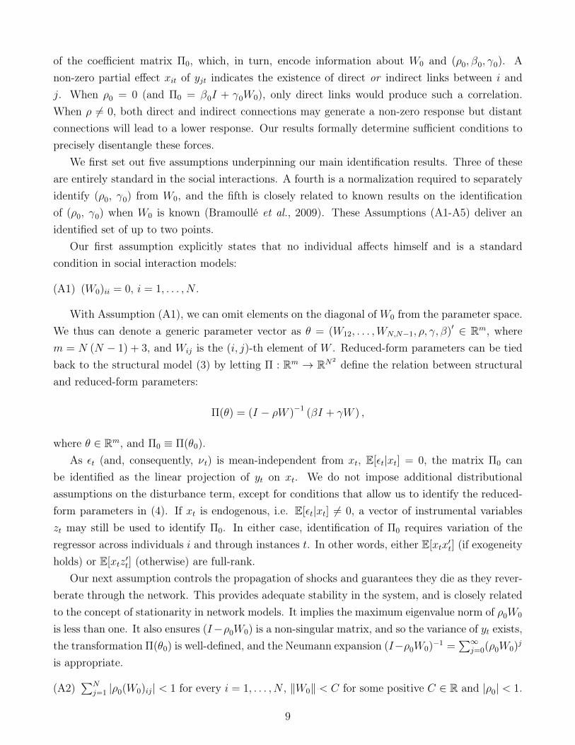
of the coefficient matrix Π0, which, in turn, encode information about W0 and (ρ0, β0, γ0). Anon-zero partial effect xit of yjt indicates the existence of direct or indirect links between i andj. When ρ0 = 0 (and Π0 = β0I + γ0W0), only direct links would produce such a correlation.When ρ 6= 0, both direct and indirect connections may generate a non-zero response but distantconnections will lead to a lower response. Our results formally determine sufficient conditions toprecisely disentangle these forces.

We first set out five assumptions underpinning our main identification results. Three of theseare entirely standard in the social interactions. A fourth is a normalization required to separatelyidentify (ρ0, γ0) from W0, and the fifth is closely related to known results on the identificationof (ρ0, γ0) when W0 is known (Bramoullé et al., 2009). These Assumptions (A1-A5) deliver anidentified set of up to two points.

Our first assumption explicitly states that no individual affects himself and is a standardcondition in social interaction models:

(A1) (W0)ii = 0, i = 1, . . . , N .

With Assumption (A1), we can omit elements on the diagonal ofW0 from the parameter space.We thus can denote a generic parameter vector as θ = (W12, . . . ,WN,N−1, ρ, γ, β)′ ∈ Rm, wherem = N (N − 1) + 3, and Wij is the (i, j)-th element of W . Reduced-form parameters can be tiedback to the structural model (3) by letting Π : Rm → RN2 define the relation between structuraland reduced-form parameters:

Π(θ) = (I − ρW )−1 (βI + γW ) ,

where θ ∈ Rm, and Π0 ≡ Π(θ0).As εt (and, consequently, νt) is mean-independent from xt, E[εt|xt] = 0, the matrix Π0 can

be identified as the linear projection of yt on xt. We do not impose additional distributionalassumptions on the disturbance term, except for conditions that allow us to identify the reduced-form parameters in (4). If xt is endogenous, i.e. E[εt|xt] 6= 0, a vector of instrumental variableszt may still be used to identify Π0. In either case, identification of Π0 requires variation of theregressor across individuals i and through instances t. In other words, either E[xtx

′t] (if exogeneity

holds) or E[xtz′t] (otherwise) are full-rank.

Our next assumption controls the propagation of shocks and guarantees they die as they rever-berate through the network. This provides adequate stability in the system, and is closely relatedto the concept of stationarity in network models. It implies the maximum eigenvalue norm of ρ0W0

is less than one. It also ensures (I−ρ0W0) is a non-singular matrix, and so the variance of yt exists,the transformation Π(θ0) is well-defined, and the Neumann expansion (I−ρ0W0)−1 =

∑∞j=0(ρ0W0)j

is appropriate.

(A2)∑N

j=1 |ρ0(W0)ij| < 1 for every i = 1, . . . , N , ‖W0‖ < C for some positive C ∈ R and |ρ0| < 1.

9

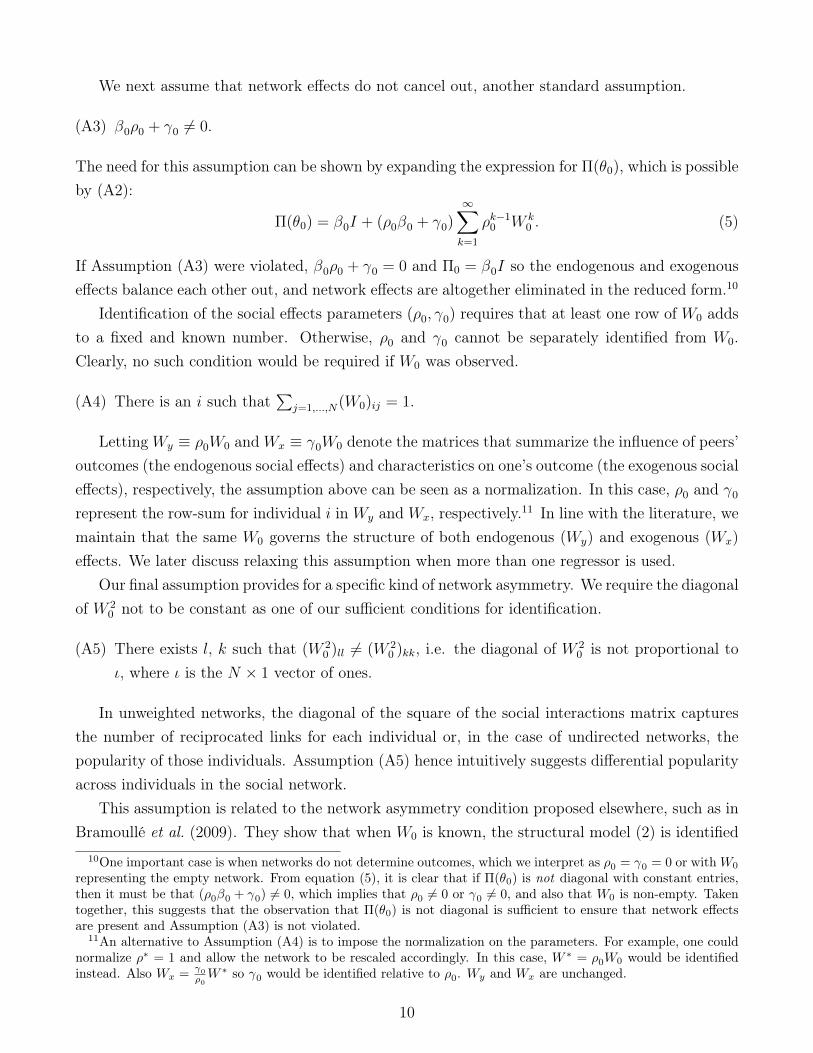
We next assume that network effects do not cancel out, another standard assumption.

(A3) β0ρ0 + γ0 6= 0.

The need for this assumption can be shown by expanding the expression for Π(θ0), which is possibleby (A2):

Π(θ0) = β0I + (ρ0β0 + γ0)∞∑k=1

ρk−10 W k

0 . (5)

If Assumption (A3) were violated, β0ρ0 + γ0 = 0 and Π0 = β0I so the endogenous and exogenouseffects balance each other out, and network effects are altogether eliminated in the reduced form.10

Identification of the social effects parameters (ρ0, γ0) requires that at least one row of W0 addsto a fixed and known number. Otherwise, ρ0 and γ0 cannot be separately identified from W0.Clearly, no such condition would be required if W0 was observed.

(A4) There is an i such that∑

j=1,...,N(W0)ij = 1.

LettingWy ≡ ρ0W0 andWx ≡ γ0W0 denote the matrices that summarize the influence of peers’outcomes (the endogenous social effects) and characteristics on one’s outcome (the exogenous socialeffects), respectively, the assumption above can be seen as a normalization. In this case, ρ0 and γ0

represent the row-sum for individual i in Wy and Wx, respectively.11 In line with the literature, wemaintain that the same W0 governs the structure of both endogenous (Wy) and exogenous (Wx)effects. We later discuss relaxing this assumption when more than one regressor is used.

Our final assumption provides for a specific kind of network asymmetry. We require the diagonalof W 2

0 not to be constant as one of our sufficient conditions for identification.

(A5) There exists l, k such that (W 20 )ll 6= (W 2

0 )kk, i.e. the diagonal of W 20 is not proportional to

ι, where ι is the N × 1 vector of ones.

In unweighted networks, the diagonal of the square of the social interactions matrix capturesthe number of reciprocated links for each individual or, in the case of undirected networks, thepopularity of those individuals. Assumption (A5) hence intuitively suggests differential popularityacross individuals in the social network.

This assumption is related to the network asymmetry condition proposed elsewhere, such as inBramoullé et al. (2009). They show that when W0 is known, the structural model (2) is identified

10One important case is when networks do not determine outcomes, which we interpret as ρ0 = γ0 = 0 or withW0

representing the empty network. From equation (5), it is clear that if Π(θ0) is not diagonal with constant entries,then it must be that (ρ0β0 + γ0) 6= 0, which implies that ρ0 6= 0 or γ0 6= 0, and also that W0 is non-empty. Takentogether, this suggests that the observation that Π(θ0) is not diagonal is sufficient to ensure that network effectsare present and Assumption (A3) is not violated.

11An alternative to Assumption (A4) is to impose the normalization on the parameters. For example, one couldnormalize ρ∗ = 1 and allow the network to be rescaled accordingly. In this case, W ∗ = ρ0W0 would be identifiedinstead. Also Wx = γ0

ρ0W ∗ so γ0 would be identified relative to ρ0. Wy and Wx are unchanged.

10

if I, W0, and W 20 are linearly independent. Given the remaining assumptions, this condition is

satisfied if (A5) is satisfied, but the converse is not true: one can construct examples in which I,W0, and W 2

0 are linearly independent when W 20 has a constant diagonal, so that Π0 does not pin

down θ0. The strengthening of this hypothesis is the formal price to pay for the social interactionsmatrix W0 being unknown to the researcher.12

Before proceeding to our formal results, we provide a very simple illustration to shed lighton how the assumptions above come together to provide identification. Suppose the observedreduced-form matrix is,

Π0 =1

455

275 310 0

310 275 0

0 0 182

,and that, following (A4), the first row is normalized to one. From the third row and column of Π0,we see there is no path of any length connecting the individual in row 3 to or from those in rows 1or 2 since her outcome is not affected by their covariates and their outcomes are not affected by hercovariates. In other words, individual 3 is isolated and (W0)13 = (W0)23 = (W0)31 = (W0)32 = 0.On the other hand, individuals 1 and 2 cannot be isolated as their covariates are correlated withthe other individual’s outcome, reflecting (A5).13 Due to the row-sum normalization of the firstrow, (W0)12 = 1. Using (A3), it can be seen that W0 is symmetric if Π0 is symmetric. We thusfind that (W0)21 = 1. This and (A1) map all elements of W0, and thus,

W0 =

0 1 0

1 0 0

0 0 0

.As the third individual is isolated, she will be only be affected by her exogenous xi and not by

12To see the strength of the assumption of Bramoullé et al. (2009) when W0 is known, choose constants c1, c2,and c3 such that c1I+c2W0+c3W

20 = 0. Focusing on diagonal elements of this condition, we see that if the diagonal

of W 20 is not proportional to the diagonal of I, then c1 = c3 = 0 because diag(W0) = 0. It follows that c2 = 0 if at

least one (off-diagonal) element of W0 is non-zero. However, the converse is not true, so that if Assumptions A1-A5do not hold, one can construct examples where Π0 does not pin down θ0. Take, for instance, N = 5 with θ0 and θwhere β = β0 = 1, ρ = 1.5, ρ0 = 0.5, γ = −2.5, γ0 = 0.5,

W0 =

0 0.5 0 0 0.5

0.5 0 0.5 0 00 0.5 0 0.5 00 0 0.5 0 0.5

0.5 0 0 0.5 0

and W =

0 0 0.5 0.5 00 0 0 0.5 0.5

0.5 0 0 0 0.50.5 0.5 0 0 00 0.5 0.5 0 0

.Both W and W0 violate (A5) ((W 2)kk = (W 2

0 )kk = 0.5 for any k), and ρ violates (A2). Nonetheless, I,W0

and W 20 are linearly independent and, likewise, so are I,W , and W 2. In this case, both parameter sets produce

Π = (I − ρ0W0)−1(β0I + γ0W0) = (I − ρW )−1(βI + γW ). This arises even as W and W0 represent very differentnetwork structures: any pair connected under W is not connected under W0 and vice-versa.

13If on the other hand, (W0)ij = 0.5, i 6= j in violation of (A5) and all agents were connected, the model wouldnot be identified.

11

endogenous or exogenous peer effects. Hence the (3, 3) element of Π0 is equal to β0 = 182455

= .4.To find ρ0, note that (I − ρ0W0)Π0 = β0I + γ0W0. Hence focussing on the (1,1) elements of thematrices above, we find that 275

455− ρ0

310455

= .4, implying ρ0 = .3 (complying with (A2)). Finally, γ0

is identified from entry (1, 2), giving γ0 = 310455− .3275

455= .5.

2.2 Main Identification Results

Under the relatively mild assumptions above, we can begin to identify parameters related to thenetwork. These results are then useful for our main identification theorems. Let λ0j denote aneigenvalue ofW0 with corresponding eigenvector v0,j for j = 1, . . . , N . Assumptions (A2) and (A3)allow us to identify the eigenvectors of W0 directly from the reduced form. As |ρ0| < 1:

Π0v0,j = β0v0,j + (ρ0β0 + γ0)∞∑k=1

ρk−10 W k

0 v0,j

=

[β0 + (ρ0β0 + γ0)

∞∑k=1

ρk−10 λk0,j

]v0,j

=β0 + γ0λ0,j

1− ρ0λ0,j

v0,j. (6)

The infinite sum converges as |ρ0λ0,j| < 1 by (A2). The equation above implies that v0,j is alsoan eigenvector of Π0 with associated eigenvalue λΠ,j =

β0+γ0λ0,j1−ρ0λ0,j

. The fact that eigenvectors ofΠ0 are also eigenvectors of W0 has a useful implication: eigencentralities may be identified fromthe reduced form, even when W0 is not identified. As detailed in de Paula (2017) and Jacksonet al. (2017), such eigencentralities often play an important role in empirical work as they allow amapping back to underlying models of social interaction.14

Now let Θ ≡ {θ ∈ Rm : Assumptions (A1)-(A5) are satisfied} be the structural parameterspace of interest. Our first theorem establishes local identification of the mapping. A parameterpoint θ0 is locally identifiable if there exists a neighborhood of θ0 containing no other θ whichis observationally equivalent. Using classical results in Rothenberg (1971), we show that ourassumptions are sufficient to ensure that the Jacobian of Π relative to θ is non-singular, which, inturn, suffices to establish local identification.

Theorem 1. Assume (A1)-(A5). θ0 ∈ Θ is locally identifiable.

An immediate consequence of local identification is that the set {θ ∈ Θ : Π(θ) = Π(θ0)} isdiscrete (i.e. its elements are isolated points). The following corollary establishes that Π is a properfunction, i.e. the inverse image Π−1(K) of any compact set K ⊂ RN2 is also compact (Krantz andParks, 2013, p. 124). Since it is discrete, the identified set must be finite.

14To identify the eigencentralities, we identify the eigenvector that corresponds to the dominant eigenvalue. IfW0

is non-negative and irreducible, this is the (unique) eigenvector with strictly positive entries, by the Perron-FrobeniusTheorem for non-negative matrices (see Horn and Johnson, 2013, p.534).

12

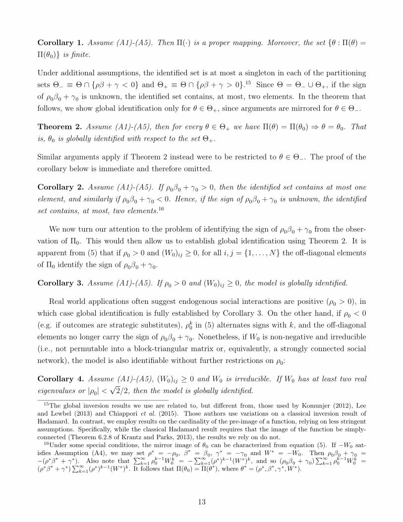
Corollary 1. Assume (A1)-(A5). Then Π(·) is a proper mapping. Moreover, the set {θ : Π(θ) =

Π(θ0)} is finite.

Under additional assumptions, the identified set is at most a singleton in each of the partitioningsets Θ− ≡ Θ ∩ {ρβ + γ < 0} and Θ+ ≡ Θ ∩ {ρβ + γ > 0}.15 Since Θ = Θ− ∪ Θ+, if the signof ρ0β0 + γ0 is unknown, the identified set contains, at most, two elements. In the theorem thatfollows, we show global identification only for θ ∈ Θ+, since arguments are mirrored for θ ∈ Θ−.

Theorem 2. Assume (A1)-(A5), then for every θ ∈ Θ+ we have Π(θ) = Π(θ0) ⇒ θ = θ0. Thatis, θ0 is globally identified with respect to the set Θ+.

Similar arguments apply if Theorem 2 instead were to be restricted to θ ∈ Θ−. The proof of thecorollary below is immediate and therefore omitted.

Corollary 2. Assume (A1)-(A5). If ρ0β0 + γ0 > 0, then the identified set contains at most oneelement, and similarly if ρ0β0 + γ0 < 0. Hence, if the sign of ρ0β0 + γ0 is unknown, the identifiedset contains, at most, two elements.16

We now turn our attention to the problem of identifying the sign of ρ0β0 + γ0 from the obser-vation of Π0. This would then allow us to establish global identification using Theorem 2. It isapparent from (5) that if ρ0 > 0 and (W0)ij ≥ 0, for all i, j = {1, . . . , N} the off-diagonal elementsof Π0 identify the sign of ρ0β0 + γ0.

Corollary 3. Assume (A1)-(A5). If ρ0 > 0 and (W0)ij ≥ 0, the model is globally identified.

Real world applications often suggest endogenous social interactions are positive (ρ0 > 0), inwhich case global identification is fully established by Corollary 3. On the other hand, if ρ0 < 0

(e.g. if outcomes are strategic substitutes), ρk0 in (5) alternates signs with k, and the off-diagonalelements no longer carry the sign of ρ0β0 + γ0. Nonetheless, if W0 is non-negative and irreducible(i.e., not permutable into a block-triangular matrix or, equivalently, a strongly connected socialnetwork), the model is also identifiable without further restrictions on ρ0:

Corollary 4. Assume (A1)-(A5), (W0)ij ≥ 0 and W0 is irreducible. If W0 has at least two realeigenvalues or |ρ0| <

√2/2, then the model is globally identified.

15The global inversion results we use are related to, but different from, those used by Komunjer (2012), Leeand Lewbel (2013) and Chiappori et al. (2015). Those authors use variations on a classical inversion result ofHadamard. In contrast, we employ results on the cardinality of the pre-image of a function, relying on less stringentassumptions. Specifically, while the classical Hadamard result requires that the image of the function be simply-connected (Theorem 6.2.8 of Krantz and Parks, 2013), the results we rely on do not.

16Under some special conditions, the mirror image of θ0 can be characterized from equation (5). If −W0 sat-isfies Assumption (A4), we may set ρ∗ = −ρ0, β

∗ = β0, γ∗ = −γ0 and W ∗ = −W0. Then ρ0β0 + γ0 =−(ρ∗β∗ + γ∗). Also note that

∑∞k=1 ρ

k−10 W k

0 = −∑∞k=1(ρ∗)k−1(W ∗)k, and so (ρ0β0 + γ0)

∑∞k=1 ρ

k−10 W k

0 =(ρ∗β∗ + γ∗)

∑∞k=1(ρ∗)k−1(W ∗)k. It follows that Π(θ0) = Π(θ∗), where θ∗ = (ρ∗, β∗, γ∗,W ∗).

13

Corollary 4 holds if there are at least two real eigenvalues, or if ρ0 is appropriately bounded.Since W0 is non-negative, it has at least one real eigenvalue, by the Perron-Frobenius Theorem. IfW0 is symmetric, for example, its eigenvalues are all real, and Corollary 4 holds. It also holds if(W0)ij ≤ 0, as we can re-write the model as ρW0 = −ρ|W0| where |W0|, is the matrix whose entriesare the absolute values of the entries in W0. In any case, the bound on |ρ0| is sufficient and holdsin most (if not all) empirical estimates we are aware of obtained from either elicited or postulatednetworks, and in our application on tax competition.

2.3 Extensions

2.3.1 Individual Fixed Effects

We observe outcomes for i = 1, . . . , N individuals repeatedly through t = 1, . . . , T instances.If t corresponds to time, it is natural to think of there being unobserved heterogeneity acrossindividuals, αi, to be accounted for when estimating Π0. The structural model (2) is then,

yit = ρ0

N∑j=1

W0,ijyjt + β0xit + γ0

N∑j=1

W0,ijxjt + αi + εit,

which can be written in matrix form as,

yt = ρ0W0yt + xtβ0 +W0xtγ0 + α∗ + εt,

where α∗ is the vector of fixed effects. Individual-specific and time-constant fixed effects can beeliminated using the standard subtraction of individual time averages. Defining yt = T−1

∑Tt=1 yt,

xt = T−1∑T

t=1 xt and εt = T−1∑T

t=1 εt,

yt − yt = ρ0W0 (yt − yt) + (xt − xt) β0 +W0 (xt − xt) γ0 + εt − εt,

if W0 is does not change with time. Identification from the reduced form follows from previoustheorems, since Π0 is unchanged when regressing yt − yt on xt − xt.17

2.3.2 Common Shocks

We next allow for unobserved common shocks to all individuals in the network in the same instancet. Such correlated effects αt can confound the identification of social interactions. As we have notplaced any distributional assumption on the covariance matrix of the disturbance term, our analysisreadily incorporates correlated effects that are orthogonal to xt. When this is not the case, one

17As is the case in panel data, this would require strict exogenity (E[εs|xt] = 0 for any s and t) or predeterminederrors (E[εs|xt] = 0 for s ≥ t) so that the matrix Π0 can be consistently estimated.

14

possibility is to model the corrected effects αt explicitly. The model then is,

yt = ρ0W0yt + xtβ0 + γ0W0xt + αtι+ εt,

where αt is a scalar capturing shocks in the network common to all individuals. Let Π01 =

(I − ρ0W0)−1 and Π02 = (β0I + γ0W0) such that Π0 = Π01Π02. The reduced-form model is,

yt = Π0xt + αtΠ01ι+ vt.

We propose a transformation to eliminate the correlated effects: exclude the individual-invariantαt, subtracting the mean of the variables at a given period (global differencing). For this purpose,define H = 1

nιι′. We note that in empirical and theoretical work it is customary to strengthen

Assumption (A4) and require that all rows of W0 sum to one if no individual is isolated (see forexample Blume et al., 2015). This strengthened assumption is usually referred to as row-sumnormalization, and is stated below:

(A4’) For all i = 1, ...N we have that∑

j=1,...,N(W0)ij = 1.

This can be written compactly asW0ι = ι. In this case,W0 can be interpreted as the normalizedadjacency matrix. Under row-sum normalization we have that,

(I −H) yt = (I −H) (I − ρ0W0)−1 (β0I + γ0W0)xt + (I −H) (I − ρ0W0)−1 εt

= (I −H) Π0xt + (I −H) vt,

because (I −H) (I − ρ0W0)−1 αtι = 0 if Assumption (A4’) holds. It then follows that Π0 =

(I −H)Π0 is identified. The next proposition shows that, under row-sum normalization of W0, Π0

is identified from Π0 (and, as a consequence, the previous results immediately apply).

Proposition 1. If W0 is diagonalizable and row-sum normalized, Π0 is identified from Π0.

Under row-sum normalization of W0, a common group-level shock affects individuals homo-geneously since (I − ρ0W0)−1αtι = αt(I + ρ0W0 + ρ2

0W20 + · · · )ι = αt

1−ρ0ι, which is a vector with

no variation across entries. Consequently, global differencing eliminates correlated effects and(I −H) (I − ρ0W0)−1 αtι = (I − ρ0W0)−1 αt (I −H) ι = 0. In the absence of row-sum normaliza-tion, global differencing does not ensure that correlated effects are eliminated. To see this, notethat (I − ρ0W0)−1 is no longer row-sum normalized and, crucially, αt(I − ρ0W0)−1ι is not a vectorwith constant entries.

The next proposition makes this point formally, that the stronger Assumption (A4’) is necessaryto eliminate group-level shocks, by showing it is not possible to construct a data transformationthat eliminates group effects in the absence of row-sum normalization.

15

Proposition 2. Define rW0 = (I − ρ0W0)−1ι. If in space Θ = {θ ∈ Rm : Assumptions (A1)-(A5)are satisfied} there are N matrices W (1)

0 , . . . ,W(N)0 such that [r

W(1)0· · · r

W(N)0

] has rank N , then

the only transformation such that (I − H)(I − ρ0W0)−1ι = 0 is H = I.

It is useful to be able to test for row-sum normalization (A4’) as it enables common shocks tobe accounted for in the social interactions model. This is possible as,

Π0ι = β0ι+ (ρ0β0 + γ0)∞∑k=1

ρk−10 W k

0 ι

=

[β0 + (ρ0β0 + γ0)

∞∑k=1

ρk−10

]ι

=β0 + γ0

1− ρ0

ι. (7)

The last equality follows from the observation that, under row-normalization of W0, W k0 ι = W0ι =

ι, k > 0. This implies Π0 has constant row-sums, which suggests row-sum normalization is testable.In the Appendix we derive a Wald test statistic to do so.18

2.3.3 Multivariate Covariates

Next, allowing for multivariate xt of dimension n× k, the reduced-form model (4) is,

yt =K∑k=1

Π0,kxk,t + νt,

where Π0,k = (I − ρ0W0)−1 (β0,k + γ0,kW0

), xk,t refers to the k-th column of xt, and β0,k and

γ0,k select the k-th element of K-dimensional β0 and γ0, respectively. The previous identificationresults then apply sequentially to each Π0,k, k = 1, . . . , K. In fact, we only then need to maintainWx = γ0W0 for one covariate. It is therefore possible to allow the structure of endogenous andexogenous social effects to differ for K − 1 of the covariates. With K covariates, equation (3) is,

yt = ρ0W0yt +K∑k=1

β0,kxt +K∑k=1

γ0,kW0,kxk,t + εt.

Let W0,k = W0 be the case for k = 1. Then, having identified ρ0 and W0 from Π0,1,

(I − ρ0W0)Π0,k = β0,kI + γ0,kW0,k,

18For ease of explanation, in the Appendix we derive the test under the asymptotic distribution of the OLSestimator. The test generally holds with minor adjustments for estimators with known asymptotic distributions.

16

for k = 2, . . . , K. The parameter β0,k then corresponds to the diagonal elements of (I − ρ0W0)Π0,k

and the off-diagonal entries correspond to the off-diagonal elements of γ0,kW0,k. If Assumption(A4) holds for every k = 1, . . . , K, we can identify γ0,k and thus W0,k for every k = 1, . . . , K.19

2.3.4 Heterogeneous β0

While many applications assume β0 to be homogeneous across individual units, we here considerpossible avenues allowing for heterogeneous coefficients. In a slight abuse of notation, consider forthis subsection β0 in equation system (3) to be diag(β01, . . . , β0N)N×N . Instead of a homogeneousscalar, β0 is a diagonal matrix with the individual-specific coefficients β01, . . . , β0N along its di-agonal. When ρ0 = 0 as in Manresa (2016), Π0 = β0 + γ0W0. In this case, under Assumption(A1), β0 is identified from the diagonal elements in Π0 and γ0W0 is identified from its off-diagonalelements.

With multiple covariates, as long as coefficients are homogeneous for one of the covariates, onecan also identify heterogeneous coefficients on the remaining covariates as done in the previousSubsection. For example, let there be K covariates and β0,k = diag(β01,k, . . . , β0N,k) for k =

1, . . . , N . Suppose β01,k = · · · = β0N,k for one of these covariates and let this k = 1 without loss ofgenerality. Having identified ρ0 and W0 from Π0,1,

(I − ρ0W0)Π0,k = β0,k + γ0,kW0,k,

for k = 2, . . . , K. Then, under Assumption (A1) , β0,k is identified from the diagonal elements in(I − ρ0W0)Π0,k and γ0,kW0,k is identified from its off-diagonal elements for k = 2, . . . , K − 1.

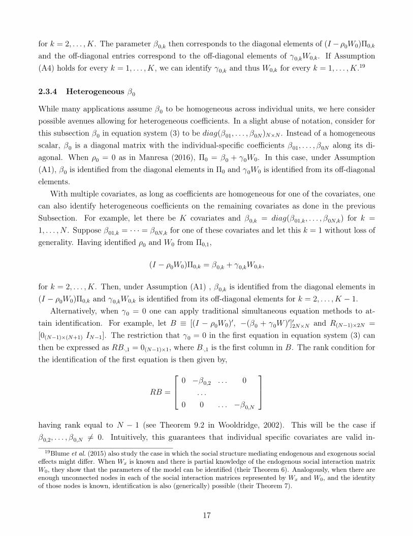
Alternatively, when γ0 = 0 one can apply traditional simultaneous equation methods to at-tain identification. For example, let B ≡ [(I − ρ0W0)′, −(β0 + γ0W )′]′2N×N and R(N−1)×2N =

[0(N−1)×(N+1) IN−1]. The restriction that γ0 = 0 in the first equation in equation system (3) canthen be expressed as RB·,1 = 0(N−1)×1, where B·,1 is the first column in B. The rank condition forthe identification of the first equation is then given by,

RB =

0 −β0,2 . . . 0

. . .

0 0 . . . −β0,N

having rank equal to N − 1 (see Theorem 9.2 in Wooldridge, 2002). This will be the case ifβ0,2, . . . , β0,N 6= 0. Intuitively, this guarantees that individual specific covariates are valid in-

19Blume et al. (2015) also study the case in which the social structure mediating endogenous and exogenous socialeffects might differ. When Wx is known and there is partial knowledge of the endogenous social interaction matrixW0, they show that the parameters of the model can be identified (their Theorem 6). Analogously, when there areenough unconnected nodes in each of the social interaction matrices represented by Wx and W0, and the identityof those nodes is known, identification is also (generically) possible (their Theorem 7).

17

strumental variables for their outcomes. Hence, if β0,1, . . . , β0,N are each different from zero,identification from Π0 is obtained.

More generally, because there are N2 equations corresponding to the entries in Π0 and, allow-ing for heterogeneity in β0 and imposing assumptions (A1)-(A5), there are N2 + 1 parameters,further restrictions (like row-sum normalization) would be necessary. We conjecture that adequaterestrictions would deliver positive identification results, but focus in the more conventional settingwith homogeneous β0.

3 Implementation

We now transition from our core identification results to their practical implementation. As this isa high-dimensional estimation problem, our preferred approach makes use of the Adaptive ElasticNet GMM (Caner and Zhang, 2014), that is based on the penalized GMM objective function. Giventhe identification results presented in Section 2, the populational version of the GMM objectivefunction will be uniquely minimized at the true parameter vector.

After setting out the estimation procedure, we showcase the method using Monte Carlo simu-lations based both on stylized random network structures as well as real world networks. In eachcase, we take a fixed network structure W0, and simulate panel data as if the data generatingprocess were given by (1). We apply the method on the simulated panel data to recover estimatesof all elements in W0, as well as the endogenous and exogenous social effect parameters.

3.1 Estimation

The parameter vector to be estimated is high-dimensional: θ = (W12, . . . ,WN,N−1, ρ, γ, β)′ ∈ Rm,where m = N (N − 1) + 3 and Wij is the (i, j)-th element of the N ×N social interactions matrixW0. To be clear, in a network with N individuals, there are N(N − 1) potential interactionsbecause individuals could interact with everyone else but herself (which would violate AssumptionA1). As a consequence, even with a modest N , there are many more parameters to estimate andm is large. For example, a network with N = 50 implies more than two thousand parametersto estimate. While we consider N (and thus m) is fixed, we still refer to θ as high-dimensional.OLS estimation requires m � NT (⇒ N � T ), so many more time periods than individuals: arequirement often met in finance data sets (van Vliet, 2018) or in other fields (see, e.g., Section 4.2in Rothenhäusler et al., 2015). Instead, to estimate a large number of parameters with limited datawe utilize high-dimensional estimation methods, that are the focus of a rapidly growing literature.However, the identification results presented in Section 2 apply more broadly and irrespective ofthe estimation procedure.

Sparsity is a key assumption underlying many high-dimensional estimation techniques. In thecontext of social interactions, we say that W0 is sparse if m, the number of non-zero elements of

18

W0, is such that m� NT . The notion of sparsity thus depends on the number of of time periods:although N and m are fixed, m itself can grow with T . Sparsity corresponds to assuming thatindividuals influence or are influenced by a small number of others, relative to the overall size ofthe potential network and the time horizon in the data. As such, sparsity is typically not a bindingconstraint in social networks analysis.20

In the estimation of sparse models, the “effective number of parameters” (or “effective degreesof freedom”) relates to the number of variables with non-zero estimated coefficients (Tibshirani andTaylor, 2012). In the context of the current social network model (and the Elastic Net estimatoron which the estimation strategy below builds on), this is approximately equivalent to the densityof the network times the number of parameters m. We then require this number to be smallerthan T . Implicitly, this calculation provides a rough assessment on the minimum required T . Forexample, with N = 30 and a network with 2% of potential links in place, this implies T should belarger than 18.

Finally, to reiterate, our identification results themselves do not depend on the sparsity ofnetworks. In particular, Assumptions (A1) to (A5) do not impose restrictions on the number oflinks in W0, or m.21

Our preferred approach estimates the interaction matrix in the reduced form while penalizingand imposing sparsity on the structural object W0. We impose sparsity and penalization in thestructural-form matrix W0 because this is a weaker requirement than imposing sparsity and penal-ization in the reduced-form matrix Π0.22 To accomplish this, we make use of the Adaptive ElasticNet GMM (Caner and Zhang, 2014), that is based on the penalized GMM objective function,

GNT (θ, p) ≡ gNT (θ)′MTgNT (θ) + p1

N∑i,j=1i 6=j

|Wi,j|+ p2

N∑i,j=1i 6=j

|Wi,j|2 (8)

where θ = (W1,2, . . . ,WN,N−1 ρ, γ, β)′ with dimension m = N(N − 1) + 3, and p1 and p2 are thepenalization terms. The term gNT (θ)′MTgNT (θ) is the unpenalized GMM objective function with

20For example, common stylized networks are sparse, such as: (i) star: all individuals receive spillovers from thesame individual; (ii) lattice: each individual is a source of spillover only to one other individual; (iii) interactions inpairs or triads or small groups, such as those described by De Giorgi et al. (2010); and (iv) small world networks(Watts, 1999). Prominent real world economic networks are also sparse. For example, in individual-level eliciteddata from AddHealth on teenage friendships (defined as reciprocated nominations), the density of links is around2% of all feasible links. In firm-level data, the density of production networks in the US is less than 1% of all feasiblelinks (Atalay et al., 2011).

21If N → ∞, Assumption (A2) would imply vanishing (W0)ij entries. As highlighted previously, we consider Nto be fixed, in line with many practical applications. Furthermore, Assumption (A2) is used to represent inversematrices as Neumann series in our identification results. What is necessary for this to hold is that a sub-multiplicativenorm on ρW be less than one. Here we use a specific norm (i.e., the maximum row sum norm), but other (induced)norms are also possible (i.e., the 2-norm or the 1-norm) (see Horn and Johnson, 2013, Chapter 5.6).

22Note that even if W is sparse, Π may not be sparse. In Appendix B.1, we show that [Π0]ij = 0 if, and only if,there are no paths between i and j in W0, and so the pair is not connected. So sparsity in Π0 is understood as W0

being ‘sparsely connected’, which is a stronger assumption than sparsity in W0.

19

moment conditions based on the orthogonality between the structural disturbance term and thecovariates: gNT (θ) =

∑Tt=1 [x1tet(θ)

′ · · · xNtet(θ)′]′, et(θ) = yt − (I − ρW )−1 (βI + γW )xt. Thereare q ≡ N2 moment conditions since xit is orthogonal to ejt, for each i, j = 1, . . . , N . Hence theGMM weight matrixMT is of dimension N2×N2, symmetric, and positive definite. For simplicity,we use MT = IN2×N2 . Note that if xt is econometrically endogenous, one can also exploit momentconditions with respect to available instrumental variables.23

Given the identification results presented in Section 2, if θ 6= θ0 and does not belong to theidentified set, then Π(θ) 6= Π(θ0). Consequently, the populational version of the GMM objectivefunction is uniquely minimized at the true parameter vector θ0.

The penalization terms in (8) is what makes this different from a standard GMM problem.The first term, p1

∑Ni,j=1,i 6=j |Wi,j|, penalizes the sum of the absolute values of Wij, i.e. the sum

of the strength of links, for all node-pairs. The second term, p2

∑Ni,j=1,i 6=j |Wi,j|2, penalizes the

sum of the square of the parameters. This term has been shown to provide better model-selectionproperties, especially when explanatory variables are correlated (Zou and Zhang, 2009). The firststage estimate is,

θ(p) = (1 + p2/T ) · arg minθ∈Rp

GNT (θ, p) (9)

where (1 + p2/T ) is a bias-correction term also used by Caner and Zhang (2014).Depending on the choice of p1, some Wi,j’s will be estimated as exact zeros. A larger share

of parameters will be estimated as zeros if p1 increases. The penalization also shrinks non-zeroestimates towards zero. A second (adaptive) step provides improvements by re-weighting thepenalization by the inverse of the first-step estimates (Zou, 2006):

θ(p) = (1 + p2/T ) · arg minθ∈Rp

gNT (θ)′MTgNT (θ) + p∗1

∑{i,j:Wij 6=0,i,j=1,...,N,

i 6=j}

|Wi,j||Wi,j|γ

+ p2

∑{i,j:Wij 6=0,i,j=1,...,N,

i 6=j}

|Wi,j|2

,

(10)where Wi,j is the (i, j)-th element of the first-step estimate of W , and we follow Caner and Zhang(2014) to set γ = 2.5. Elements Wi,j estimated as zeros in the first stage are kept as zero in thesecond stage, because Wi,j = 0 implies the effective penalization is infinite. We write p = (p1, p

∗1, p2)

as the final set of penalization parameters. Conditional on p, the estimate of the Adaptive ElasticNet GMM procedure is θ(p). Finally, we update the estimates of ρ0, β0 and γ0 on a regressionusing peers-of-peers as instruments, similar to Bramoullé et al. (2009), but using the network asestimated in (10). This final step is not necessary but performs better in small samples. As inCaner and Zhang (2014, p. 35), the penalization parameters p are chosen by the BIC criterion.

23For expositional ease, we describe estimation in the context of the reduced form model (4), thereby abstainingfrom individual fixed or correlated effects. As the GMM estimator uses moments between the structural disturbanceterms and covariates, this endogeneity is built into the estimation procedure.

20

This balances model fit with the number of parameters included in the model.24

In Appendix B.2 we provide further implementation details, including the choice of initialconditions. Of course, other estimation methods are available and our identification results do nothinge on any particular estimator. Our aim is to demonstrate the practical feasibility of usingthe Adaptive Elastic Net estimator, rather than claim it is the optimal estimator.25 Indeed, inAppendix B.3 we show how OLS can also be used to estimate θ if T is sufficiently large. Thismakes precise the benefits of penalized estimation for any given T and highlights that sparsity isnot required for our identification results.

3.2 Simulations

We showcase the method using Monte Carlo simulations based both on stylized random networkstructures as well as real world networks. We describe the simulation procedures, results androbustness checks in more detail in the Appendix. Here we just provide a brief overview tohighlight how well the method works to recover social networks even in relatively short panels.

For each simulated network, we take a fixed network structure W0, and simulate panel dataas if the data generating process were given by (1). We then apply the method on the simulatedpanel data to recover estimates of all elements in W0, as well as the endogenous and exogenoussocial effect parameters (ρ0, γ0). Our result identifies entries in W0 and so naturally recovers linksof varying strength. It is long recognized that link strength might play an important role in socialinteractions (Granovetter, 1973). Data limitations often force researchers to postulate some ties tobe weaker than others (say, based on interaction frequency). In contrast, our approach identifiesthe continuous strength of ties, W0,ij, where W0,ij > 0 implies node j influences node i.

The stylized networks we consider are a random network, and a political party network in whichtwo groups of nodes each cluster around a central node. The real world networks we consider arethe high-school friendship network in Coleman (1964) from a small high school in Illinois, andone of the village networks elicited in Banerjee et al. (2013) from rural Karnataka, India. Thesenetworks vary in size, complexity, and their aggregate and node-level features. All four networksare also sparse. For the stylized networks, we first assess the performance of the estimator for afixed network size, N = 30. We simulate the real-world networks using non-isolated nodes in each

24Following Caner and Zhang, 2014, the choice of p, which we denote as p, is the one that minimizes

BIC(p) = log

[gNT

(θ(p)

)′MT gNT

(θ(p)

)]+A

(θ(p)

)· log T

T

where A(θ(p)

)counts the number of non-zero coefficients among {W1,2, . . . ,WN,N−1}. (See also Zou et al., 2007.)

25For example, Manresa (2016) also relies on a Lasso-related methodology but restricts ρ0 to be zero and soignores endogenous social effects. If instrumental variables are available, Lam and Souza (2016) propose estimating(1) directly using the Adaptive Lasso and exploiting sparsity of the estimated W0. Gautier and Rose (2016) extendthe (identification-robust) Self-Tuning Instrumental Variable estimator in Gautier and Tsybakov (2014).

21

(so N = 70 and 65 respectively).26

Despite the heterogeneity across networks, the method performs well in all simulations: FigureA1 shows the simulation results. Each Panel presents a different metric as we vary T for eachsimulated network. Panel A shows that for each network, the proportion of zero entries in W0

correctly estimated as zeros is above 90% even when T = 5. The proportion approaches 100% asT grows. Conversely, Panel B shows the proportion of non-zeros entries estimated as non-zeros isalso high for small T . It is above 70% from T = 5 for the Erdos-Renyi network, being at least85% across networks for T = 25, and increasing as T grows. As discussed above, the AdaptiveElastic Net estimator is better in recovering true zero entries because it is a well-known featurethat shrinkage estimators tend to shrink small parameters to zero.

Panels C and D show that for each simulated network, the mean absolute deviation betweenestimated and true networks for W and Π falls quickly with T and is close zero for large samplesizes. Finally, Panels E and F show that biases in the endogenous and exogenous social effectsparameters, ρ and γ, also fall quickly in T . The fact that biases are not zero is as expected forsmall T , being analogous to well-known results for autoregressive time series models.27

In the Appendix we show the robustness of the simulation results to: (i) varying network sizesand node definitions in the real work network of Banerjee et al. (2013); (ii) alternative parameterchoices and richening up the structure of shocks across nodes. We demonstrate the gains fromusing the Adaptive Elastic Net GMM estimator over alternative estimators, such as the AdaptiveLasso estimator and OLS, and also show how incorporating partial knowledge on W0 provides forperformance gains.

4 Application: Tax Competition Between US States

Our identification result can be used to shed new light on a classic social interactions problem:tax competition between US states (Wilson, 1999). Since the seminal empirical studies in taxcompetition between jurisdictions (Case et al., 1989; Case et al., 1993), it has been well-recognizedthat defining competing ‘neighbors’ is the central empirical challenge, and theory cannot resolve theissue. Two mechanisms have been argued to drive the structure of interactions across jurisdictions:factor mobility and yardstick competition.

On factor mobility, Tiebout (1956) first argued that labor and capital can move in response todifferential tax rates across jurisdictions. Factor mobility leads naturally to the postulated socialinteractions matrix being: (i) geographic neighbors given labor mobility; and (ii) jurisdictions withsimilar economic or demographic characteristics, given capital mobility (Case et al., 1989).28

26As in Bramoullé et al., 2009, we exclude isolated nodes because they do not conform with row-sum normalization.27The bias in spatial auto-regressive models with small number of observations even when the network is observed

is similarly documented by Mizruchi and Neuman (2008), Farber et al. (2009), Smith (2009), Neuman and Mizruchi(2010), and Wang et al. (2014).

28A body of evidence finds that tax bases are mobile in response to tax differentials (Hines, 1996; Devereux and

22

A second mechanism occurs through political economy channels (Shleifer, 1985). In particular,yardstick competition between jurisdictions is driven by voters making comparisons between statesto learn about their own politician’s quality. Besley and Case (1995) formalize the idea in amodel where voters use taxes set by governors in neighboring states to infer their own governor’squality. This generates informational externalities across jurisdictions, forcing incumbents intoyardstick competition, where their tax setting behavior is determined by what other incumbentsdo. Yardstick competition leads naturally to the postulated interactions matrix corresponding toa matrix of ‘political neighbors’: other states that voters make comparisons to.

This application shows the practical use of our approach to recover social interactions in asetting in which the number of nodes and time periods is relatively low: the data covers mainlandUS states, N = 48, for years 1962-2015, T = 53. Our approach identifies the structure of socialinteractions among ‘economic neighbors’, that we denote Wecon. We contrast this against a nullhypothesis that states are only influenced by their geographic neighbors, Wgeo, as postulated byBesley and Case, 1995 and shown in Figure 1A. With Wecon recovered, we can establish, beyondgeography, what predicts the existence and strength of ties between states. Finally, relative toWgeo, we conduct simulations using Wecon to assess the equilibrium propagation of tax settingshocks across mainland US states. Taken together, this body of evidence allows us to providenovel insights related to the role of factor mobility and yardstick competition in driving tax settingbehavior across US states.

4.1 Data and Empirical Specification

We denote state tax liabilities for state i in year t as τ it, covering state taxes collected from real percapita income, sales and corporate taxes. We measure this using a series constructed from datapublished annually in the Statistical Abstract of the United States. Our series covers mainlandstates (N = 48) for years 1962-2015, (T = 53), therefore extending the sample used by Besley andCase (1995), that runs from 1962-1988 (T = 26).29 The outcome considered, ∆τ it, is the changein tax liabilities between years t and (t− 2) because it might take a governor more than a year toimplement a tax program. Their model implies a standard social interactions specification for thetax setting behavior of state governors:

∆τ it = ρ

N∑j=1

W0,ij∆τ jt + γ

N∑j=1

W0,ijxjt + βxit + αi + αt + εit. (11)

Griffith, 1998; Kleven et al., 2013, 2014)29Besley and Case (1995) test their political agency model using a two equation set-up: (i) on gubernatorial

re-election probabilities; and (ii) on tax setting. Our application focuses on the latter because this represents asocial interaction problem. They use two tax series: (i) TAXSIM data (from the NBER) which runs from 1977-88;and (ii) state tax liabilities series constructed from data published annually in the Statistical Abstract of the USthat runs from 1962-1988. All their results are robust to either series. We extend the second series.

23

Tax setting behavior is thus determined by (i) endogenous social effects arising through neighbors’tax changes (

∑Nj=1W0,ij∆τ jt); (ii) exogenous social effects arising through the economic/demographic

characteristics of neighbors (∑N

j=1W0,ijxjt); (iii) state i’s characteristics (xit), that include incomeper capita, the unemployment rate, and the proportion of young and elderly. All specificationsinclude state and time effects (αi, αt), so allowing for time-invariant unobserved heterogeneityacross states, and for common (macroeconomic) shocks. Due to the inclusion of the time effectsαt, we normalize the rows of Wecon to one. Table A7 presents descriptive statistics for the Besleyand Case (1995) sample and our extended sample.

Much of the earlier literature focuses on endogenous social effects and ignores exogenous socialeffects by setting γ = 0. Our identification result allows us to relax this constraint and thusestimate the full typology of social effects described by Manski (1993). This is important becauseonly endogenous social effects lead to social multipliers, and are crucial to identify as they canlead to a race-to-the-bottom or sub-optimal public goods provision (Brennan and Buchanan, 1980;Wilson, 1986; Oates and Schwab, 1988).

After estimating the neighborhood matrix, we follow Besley and Case (1995) and estimate themodel instrumenting for ∆τ jt using neighbors’ lagged change in income per capita, and neighbors’lagged change in unemployment rate. These instruments are in the spirit of using exogenous socialeffects to instrument for neighbor’s tax changes. However, given our approach allows us to estimateexogenous social effects (γ 6= 0), these instruments will generally be weaker when estimating thefull specification in (11). We thus follow Bramoullé et al. (2009) and De Giorgi et al. (2010), andalso instrument neighbors’ tax changes with neighbor-of-neighbor characteristics.

4.2 Preliminary Findings

Table 1 presents our preliminary findings and comparison to Besley and Case (1995). Column 1shows OLS estimates of (11) where the postulated social interactions matrix is based on geographicneighbors, exogenous social effects are ignored so γ = 0 and the panel includes all 48 mainlandstates but runs only from 1962-1988 as in Besley and Case (1995). Social interactions influencegubernatorial tax setting behavior: ρOLS = .375. Column 2 shows this to be robust to instrument-ing neighbors’ tax changes using the instrument set proposed by Besley and Case (1995). ρ2SLS ismore than double the magnitude of ρOLS suggesting tax setting behaviors across jurisdictions arestrategic complements, and OLS estimates are heavily downward-biased.

Columns 3 and 4 replicate both specifications over the longer sample period, and confirm Besleyand Case’s (1995) finding on social interactions to be robust in this longer sample. We again notethat ρ2SLS is more than double the magnitude of ρOLS. The result in Column 4 implies that forevery dollar increase in the average tax rates among geographic neighbors, a state increases itsown taxes by 61 cents. This is similar to the headline estimate of Besley and Case (1995).30

30Nor is the magnitude very different from earlier work examining fiscal expenditure spillovers. For example,

24

4.3 Endogenous and Exogenous Social Interactions (ρ and γ)

We now move beyond much of the earlier political economy and public economics literature to firstestablish whether there are endogenous and exogenous social interactions in tax setting behavior.We first focus on the endogenous and exogenous social interaction parameters, and in the nextsubsection we detail the identified social interactions matrix, Wecon. Column 1 of Table 2 shows theinitial estimates obtained from the Adaptive Elastic Net procedure where γ = 0. Columns 2 and3 show the resulting OLS and 2SLS estimates for ρ: ρ2SLS = .641 > ρOLS = .378 > 0.31 Columns4 to 6 estimate the full model in (11). Columns 5 and 6 show the OLS and 2SLS estimates ofρ are smaller, and less precisely estimated when exogenous social effects are allowed. This is notsurprising given that the instrument set is based on neighbors’ characteristics, many of which aredirectly controlled for in (11), thus reducing the effective variation induced by the instrument.Hence, in Column 7, we report 2SLS estimates based on instruments using neighbor-of-neighborcharacteristics. This represents our preferred specification: ρ2SLS = .608 (with a standard error of.220). This value also meets the requirements on ρ in Corollaries 3 and 4 for global identification.

In short, there is robust evidence of endogenous social interactions in tax setting behavior ofgovernors across states.32

4.4 Identified Social Interactions Matrix (Wecon)

Figure 1B shows how the structure of economic (Wecon) and geographic networks (Wgeo) differ,where connected edges imply that two states are linked in at least one direction (either state icausally impacts state taxes in j, and/or vice versa). This comparison makes it clear whetherall states geographically adjacent to i matter for its tax setting behavior and whether there arenon-adjacent states that influence its tax rate.

The left-hand panel of Figure 1B shows the network of geographic neighbors (whose edgesare colored blue), onto which we have superimposed the edges that are not identified as links inWecon; these dropped edges are indicated in red. This first implies that not all geographicallyadjacent states are relevant for tax setting behavior. The right-hand panel of Figure 1B adds newedges identified in Wecon that are not part of Wgeo. These represent non-adjacent states throughwhich social interactions occur. This implies the existence of spatially dispersed social interactionsbetween states. The implication is that for tax-setting behavior, economic distance is imperfectlymeasured if we simply assume that interactions depend only on geographical distance. As detailed

Case et al. (1989) find that US state government levels of per-capita expenditures are significantly impacted bythe expenditures of their neighbors, with the size of the impact being that a one dollar increase in neighbors’expenditures leads to an increase in own-state expenditures by seventy cents.

31We report robust standard errors and so do not adjust them for the fact that Wecon is estimated.32Table A8 shows the full set of exogenous social effects (so Columns 1 to 4 refer to the same specifications as

Columns 4 to 7 in Table 2). Exogenous social effects operate through economic neighbors’ income per capita andunemployment rate. Demographic characteristics of economic neighbors to state i do not impact its tax rate.

25

below, this has many implications for the economics of tax competition.As Table 3 summarizes, Wgeo has 214 edges, while Wecon has only 144 edges. States are less

connected than implied by postulating geographic networks. Wecon and Wgeo have 79 edges incommon. However, Wgeo has 135 edges that are absent in Wecon. Hence, while geography remainsa key determinant of tax competition, the majority of geographical neighbors (135/214 = 63%)are not relevant for tax setting. There are 65 edges that exist only in Wgeo, so although there arefewer edges in Wecon, the identified social interactions are more spatially dispersed than under theassumption of geographic networks. This is reflected in the far lower clustering coefficient in Wecon

than in Wgeo (.026 versus .194).33

4.5 Strength of Ties and Reciprocity

Our estimation strategy identifies the continuous strength of ties, W0,ij, where W0,ij > 0 is inter-preted as state j influencing outcomes in state i. This is useful because recent developments intax competition theory, using insights from the social networks literature, suggest links need notbe reciprocal or of symmetric strength (Janeba and Osterleh, 2013).

Figure 2A shows the distribution of W0,ij’s across edges in Wecon (conditional on W0,ij > 0).The strength of ties between pairs of states varies greatly. The mean strength of ties is .19, thatis higher than the median strength, .085, suggesting many weak ties. At the other end of thedistribution, the strongest 10% of ties have weight above .6.

On the reciprocity of ties, Table 3 reveals that only 29.2% of edges in Wecon are reciprocal (alledges in Wgeo are reciprocal by construction). Hence, tax competition is both spatially disperseand highly asymmetric. In most cases where tax setting in state i is influenced by taxes in statej, the opposite is not true.

Panels B and C in Figure 2 illustrate this for California, indicating the strength of each tie(Wecon,CA,j). Figure 2B shows the in-network for California: those states causally impacting tax-setting in California. Some geographic neighbors to California influence its tax setting behavior(Nevada and Oregon), although these ties are weak. On the other hand, non-adjacent statesinfluence California (Colorado, Maine), and these in-network ties are stronger than geographicallyadjacent in-network ties. Figure 2C shows the out-network for California, again indicating each tiestrength (Wecon,i,CA): those states whose taxes are influenced by taxes in California. We see thatnone of the geographic neighbors to California are influenced by its tax setting behavior, whereasa number of non-adjacent states are influenced (including East Coast states such as Virginia, andSouthern states, such as Louisiana). When states are influenced by taxes in California, these tiestend to be relatively strong: Wecon,i,CA > .19 for all five in-network ties.

33The clustering coefficient is the frequency of the number of fully connected triplets over the total number oftriplets. Other metrics can also be used to provide a scalar comparison of Wgeo and Wecon. One way to do so isto reshape both matrices as vectors of length (48 × 47) and to compute their correlation. Doing so, we obtain acorrelation coefficient of .322.

26

Given common time shocks αt in (11), row-sum normalization is required and ensures∑

jW0,ij =

1. Hence, for every state i there will be at least one economic neighbor state j∗ impacts it, so thatW0,ij∗ > 0. This just reiterates that social interactions matter. On the other hand, our procedureimposes no restriction on the derived columns of Wecon. It could be that a state does not affect anyother state. Examining this possibility directly in Wecon, we see this occurs for Minnesota, NewJersey, New Mexico, Vermont, and Wisconsin. These states have an out-degree of zero. Their taxrates impact no other states.

Table 3 reports the degree distribution across all nodes (states), splitting for in-networks andout-networks. In Wgeo, the in-degree is by construction equal to the out-degree, as all ties arereciprocal. The greater sparsity of the network of economic neighbors is again reflected in thedegree distribution being lower for Wecon than for Wgeo. In Wecon the dispersion of in- and out-degree networks is very different (as measured by the standard deviation), being near double forthe in-degree. This asymmetry in Wecon further suggests that some highly focal or influential statesdrive tax setting behavior in other states.

Figures 3A and 3B show complete histograms for the in- and out-degree across states. Thehistogram on the left is for in-degree, and shows that states under Wecon generally have lowerin-degree than under Wgeo. The states that are influenced by the highest number of other statesare Utah, Pennsylvania and Ohio. The histogram on the right for out-degree, shows the five statesdescribed above that do not impact other states (Wisconsin, Vermont, New Mexico, New Jerseyand Minnesota). Delaware is an outlier influential state in its out-degree in determining tax settingin other states: as discussed below, Delaware is a well-known potential tax haven.34

4.6 Factor Mobility or Yardstick Competition?

We conclude by presenting two strategies to shed light on whether factor mobility and yardstickcompetition drive these social interactions: (i) exploiting information in the identified social inter-actions matrix Wecon; (ii) following Besley and Case (1995), using gubernatorial re-election as anindirect test of the relevance of yardstick competition.

In our first strategy we estimate the factors correlated with the existence/strength of linksbetween states i and j in Wecon using the following dyadic regression:

Wecon,ij = λ0 + λ1Xij + λ2Xi + λ3Xj + uij.

We discretize link strength so Wecon,ij ∈ {0, 1} and predict the existence of a link using a linearprobability model. We then estimate the correlates of link strength Wecon,ij ∈ [0, 1] using a Tobit

34Dyreng et al. (2013) find that taxes play an important role in determining whether firms locate subsidiaries inDelaware: a Delaware-based state tax avoidance strategy lowers state effective tax rates by around 1 percentagepoint. They also report that in June 2010, Delaware landed at the top of National Geographic magazine’s publishedlist of the most secretive tax havens in the world (ahead of foreign tax havens such as Luxembourg, Switzerland,and the Cayman Islands).

27

model. The elements Xij, Xi, and Xj correspond to characteristics of the pair of states (i, j), ofstate i, and state j, respectively. Covariates are time-averaged over the sample period, and robuststandard errors are reported. The sample thus corresponds to N × (N − 1) = 48 × 47 = 2256

potential ij links that could have formed.Table 4 presents the results. Column 1 controls only for whether states i and j are geographic

neighbors. This is highly predictive of a link between them. Columns 2 and 3 show that distancebetween states also negatively correlates with them being linked, but that when both geographicadjacency and distances are included, the former is more predictive. Hence, we control only forwhether i and j are geographic neighbors in the remaining Columns.

The next set of specifications use the insight that economic neighbors are likely to be basedon a mixture of similarity in geography, income per capita, and demography (Case et al., 1989).Column 4 thus adds two Xij covariates to capture the economic and demographic homophilybetween states i and j. GDP homophily is the absolute difference in the states GDP per capita.Demographic homophily is the absolute difference of the share of young people (aged 5-17) plusthe absolute difference of the share of elderly people (aged 65+) across the states. GDP homophilypredicts ties, whereas demographic homophily does not.

Columns 5 to 7 then sequentially add in several sets of controls. For labor mobility, we usenet state-to-state migration data to control for the net migration flow of individuals from state ito state i (defined as the flow from i to j minus the flow from j to i).35 We then add a politicalhomophily variable between states. For any given year, this is set to one if a pair of states havegovernors of the same political party. As this is time averaged over our sample, this elementcaptures the share of the sample period in which the states have governors of the same party.Lastly, we include whether state j is considered a tax haven (and so might have disproportionateinfluence on other states). Based on Findley et al. (2012), the following states are coded as taxhavens: Nevada, Delaware, Montana, South Dakota, Wyoming and New York. This corroboratesearlier evidence in Figure 3B, where Delaware, Wyoming and Nevada were among the states withthe highest out-degree.

The specification in Column 7 shows that with this full set of controls, geographic adjacencyremains a robust predictor of the existence of links between states. However, the identified economicnetwork highlights additional significant predictors of tax competition between states: politicalhomophily reduces the likelihood of a link, suggesting any yardstick competition driving socialinteractions occurs when voters compare their governor to those of the opposing party in otherstates. The tax haven states appear to be especially influential in the tax setting behaviors of other

35We also experimented with alternative measures of labor migration, and results were qualitatively the same.State-to-state migration data are based on year-to-year address changes reported on individual income tax re-turns filed with the IRS. The data cover filing years 1991 through 2015, and include the number of returns filed,which approximates the number of households that migrated, the number of personal exemptions claimed, whichapproximates the number of individuals who migrated. The data are available at https://www.irs.gov/statistics/soi-tax-stats-migration-data (accessed September 2017).

28

states. The strong influence of tax haven states might lead to a race-to-the-bottom. Relative tothese factors, the economic and demographic similarity between states play an insignificant role indetermining interactions between states.

The final column considers the continuous link strength as an outcome and reports Tobit partialaverage effect estimates. This reinforces that geography, political homophily, and tax haven statusall robustly correlate to the strength of influence states tax setting has on others. Labor mobilitybetween states does not robustly predict either the existence or strength of ties.

Our second strategy to investigate factor mobility and yardstick competition follows the in-tuition of Besley and Case (1995). They suggest an indirect test of the relevance of yardstickcompetition is that this mechanism only applies to governors not facing term limits. Therefore wecompare our main effects across two subsamples: state-years in which the governor can and cannotrun for reelection. The results are reported in Table 5. The 2SLS results suggest that in bothsamples, endogenous social interaction effects exist, although they are more precisely estimatedwhen governors can run for re-election.

Taken together, our evidence suggests that both factor mobility (of both labor and capital,as measured through the influence of tax havens), and yardstick competition (occurring throughcomparisons to governors of the other party), are important mechanisms driving the existence andstrength of interactions in tax-setting behavior across US states.

Finally, in the Appendix, we contrast how shocks to tax setting in a given state propagateunder the identified interactions matrix Wecon, relative to what would have been predicted under apostulated network structure based on Wgeo. As Wecon is spatially more dispersed than Wgeo, thegeneral equilibrium effects might be very different under the two network structures. We thereforediscuss the implications for tax inequality under Wecon and the Wgeo counterfactual.

5 Discussion

In a canonical social interactions model, we provide sufficient conditions under which the socialinteractions matrix, and endogenous and exogenous social effects are all globally identified, evenabsent information on social links. Our identification strategy is novel, and may bear fruit inother areas. We describe how high-dimensional estimation techniques can be used to estimatethe model based on the Adaptive Elastic Net GMM method. We showcase our method in MonteCarlo simulations using two stylized and two real world networks: these highlight that even inpanels as short as T = 5, the majority of social ties can be correctly identified. Finally, weemploy this estimation strategy to provide novel insights in a classic social interactions problem:tax competition across US states.

Our method is immediately applicable to other classic social interactions problems. For exam-ple, in finance a long-standing question has been whether CEOs are subject to relative performance

29

evaluation, and if so, what is the comparison set of firms/CEOs used (Edmans and Gabaix, 2016).36

Other fields such as macroeconomics, political economy and trade are all obvious areas where so-cial interactions across jurisdictions/countries etc. could drive key outcomes, panel data exist, andthe number of nodes is relatively fixed. Our approach can also be applied to new contexts wheresocial interactions determine economic behavior but data on social links is absent. Advances inthe availability of administrative data, data from social media or mobile technologies, and highfrequency data in finance and from online economic transactions, all offer new possibilities to iden-tify social interactions. For example, van Vliet (2018) studies the interconnectedness between thelargest financial institutions in during the 2008 financial crisis using readlily available market data,in which N = 13 and T = 500.

Three further directions for future research are of note. First, under partial observability ofW0 (as in Blume et al., 2015), the number of parameters in W0 to be retrieved falls quickly. Ourapproach can then still be applied to complete knowledge of W0, such as if Aggregate RelationalData is available, and this could be achieved with potentially weaker assumptions for identification,and in even shorter panels. To illustrate possibilities, Figure 4 shows results from a final simulationexercise in which we assume the researcher starts with partial knowledge of W0. We do so for theBanerjee et al. (2013) village family network, showing simulation results for scenarios in which theresearcher knows the social ties of the three (five, ten) households with the highest out-degree. Forcomparison we also show the earlier simulation results when W0 is entirely unknown. This clearlyillustrates that with partial knowledge of the social network, performance on all metrics improvesrapidly for any given T .

Second, we have developed our approach in the context of the canonical linear social interactionsmodel (1). This builds on Manski (1993) when W0 is known to the researcher, and the reflectionproblem is the main challenge in identifying endogenous and exogenous social effects. However, asestablished in Blume et al. (2011) and Blume et al. (2015), the reflection problem is functional-formdependent and may not apply to many non-linear models. An important topic for future researchis thus to extend the insights gathered here to non-linear social interaction settings.

Finally, our approach has taken the network structure as predetermined and fixed. Clearly, animportant part of the social networks literature examines endogenous network formation (Jacksonet al., 2017; de Paula, 2017). Our analysis allows us to begin probing the issue in two ways. First,the kind of dyadic regression analysis in Section 4 on the correlates of entries in W0,ij suggests fac-

36Edmans and Gabaix (2016) overview the theory and empirics of executive compensation. Applying the infor-mativeness principle in contract theory to CEO pay suggests peer performance is informative about the degree towhich firm value is due to high CEO effort or luck. In a first generation of studies, Aggarwal and Samwick (1999)and Murphy (1999) showed that CEO pay is determined by absolute, rather than relative performance. However,this conclusion has been challenged by others such as Gong et al. (2011) who argue these conclusions arise fromidentifying relative performance evaluation (RPE) based on an implicit approach, assuming a peer group (e.g. basedon industry and/or size). Indeed, when Gong et al. (2011) study the explicit use of RPE, based on the disclosureof peer firms and performance measures mandated by the SEC in 2006, they actually find that 25% of S&P 1500firms explicitly using RPE. We are currently working on using our method to provide novel evidence on the matter.

30

tors driving link formation and dissolution. Second, it is possible to examine whether the identifiedsocial interactions matrix is stable over time. To illustrate the possibility in a real world setting,we extend our application on tax competition to investigate the stability of Wecon by running theprocedure in two subsamples, each with T = 26 periods: 1962-88 and 1989-2015. Panels A andB in Figure 5 shows the resulting estimated economic networks in each subsample, and Panel Cprovides network statistics for each subsample panel (as well as for the earlier estimated economicnetwork and the network based on geographic neighbors). This highlights that the network struc-ture of tax competition has changed over time, with the later sample network from 1989-2015having fewer edges, fewer reciprocated edges, lower clustering and lower degree distribution.

This analysis leads naturally to a broad agenda going forward, to address the challenge ofsimultaneously identifying and estimating time varying models of network formation and socialinteraction, all in cases where data on social networks is not required.

References

Acemoglu, D., V. Carvalho, A. Ozdaglar, and A. Tahbaz-Salehi (2012). The NetworkOrigins of Aggregate Fluctuations. Econometrica, 80, 1977–2016.

Aggarwal, R. K. and A. A. Samwick (1999). Executive Compensation, Strategic Competition,and Relative Performance Evaluation: theory and evidence. The Journal of Finance, 54.

Ambrosetti, A. and G. Prodi (1972). On the Inversion of Some Differentiable Mappings withSingularities between Banach Spaces. Annali di Matematica Pura ed Applicata, 93, 231–46.

——— (1995). A Primer of Nonlinear Analysis, Cambridge University Press.

Anselin, L. (2010). Thirty Years of Spatial Econometrics. Papers in Regional Science, 89, 3–25.

Atalay, E., A. Hortacsu, J. Roberts, and C. Syverson (2011). Network Structure ofProduction. Proceedings of the American Mathematical Society, 108, 5199–202.

Ballester, C., A. Calvo-Armendol, and Y. Zenou (2006). Who’s Who in Networks.Wanted: The Key Player. Econometrica, 74, 1403–17.

Banerjee, A., A. G. Chandrasekhar, E. Duflo, and M. O. Jackson (2013). The Diffusionof Microfinance. Science, 341, 1236498.

Barrenho, E., M. Miraldo, C. Propper, and C. Rose (2019). Peer and Network Effects inMedical Innovation: The Case of Laparoscopic Surgery in the English NHS. University of YorkWorking Paper.

31

Battaglini, M., E. Patacchini, and E. Rainone (2019). Endogenous Social Connections inLegislatures. NBER Working Paper 25988.

Besley, T. and A. Case (1994). Unnatural Experiments? Estimating the Incidence of Endoge-nous Policies. NBER Working Paper 4956.

——— (1995). Incumbent Behavior: Vote-seeking, Tax-setting, and Yardstick Competition. Amer-ican Economic Review, 85, 25–45.

Blume, L., W. A. Brock, S. N. Durlauf, and Y. Ioannides (2011). Identification of SocialInteractions. in Handbook of Social Economics, ed. by J. Behabib, A. Bisin, and M. O. Jackson,Noth-Holland, vol. 1B.

Blume, L. E., W. A. Brock, S. N. Durlauf, and R. Jayaraman (2015). Linear SocialInteractions Models. Journal of Political Economy, 123, 444–96.

Bonaldi, P., A. Hortacsu, and J. Kastl (2015). An Empirical Analysis of Funding CostsSpillovers in the EURO-zone with Application to Systemic Risk. Princeton University WorkingPaper.

Bramoullé, Y., H. Djebbari, and B. Fortin (2009). Identification of Peer Effects ThroughSocial Networks. Journal of Econometrics, 150, 41–55.

Brennan, G. and J. Buchanan (1980). The Power to Tax: Analytical Foundations of a FiscalConstitution, Cambridge University Press.

Breza, E., A. Chandrasekhar, T. McCormick, and M. Pan (2019). Using AggregatedRelational Data to Feasibly Identify Network Structure without Network Data. American Eco-nomic Review.

Bursztyn, L., F. Ederer, B. Ferman, and N. Yuchtman (2014). Understanding Mech-anisms Underlying Peer Effects: Evidence From a Field Experiment on Financial Decisions.Econometrica, 82, 1273–301.

Caner, M. and H. H. Zhang (2014). Adaptive Elastic Net for Generalized Method of Moments.Journal of Business and Economic Statistics, 32, 30–47.

Case, A., J. R. Hines, and H. S. Rosen (1989). Copycatting: Fiscal Policies of States andTheir Neighborrs. NBER Working Paper 3032.

Case, A., H. Rosen, and J. Hines (1993). Budget Spillovers and Fiscal Policy Interdependence:Evidence from the States. Journal of Public Economics, 52, 285–307.

Chandrasekhar, A. and R. Lewis (2016). Econometrics of Sampled Networks. Working Paper.

32

Chaney, T. (2014). The Network Structure of International Trade. American Economic Review,104, 3600–34.

Chiappori, P.-A., I. Komunjer, and D. Kristensen (2015). Nonparametric Identificationand Estimation of Transformation Models. Journal of Econometrics, 188, 22–39.

Coleman, J. S. (1964). Introduction to Mathematical Sociology, London Free Press Glencoe.

Conley, T. G. and C. R. Udry (2010). Learning About a New Technology: Pineapple inGhana. American Economic Review, 100, 35–69.

De Giorgi, G., M. Pellizzari, and S. Redaelli (2010). Identification of Social Interactionsthrough Partially Overlapping Peer Groups. American Economic Journal: Applied Economics,2, 241–75.

de Marco, G., G. Gorni, and G. Zampieri (2014). Global Inversion of Functions: an Intro-duction. ArXiv:1410.7902v1.

de Paula, A. (2017). Econometrics of Network Models. in Advances in Economics and Econo-metrics: Theory and Applications, ed. by B. Honore, A. Pakes, M. Piazzesi, and L. Samuelson,Cambridge University Press.

Devereux, M. and R. Griffith (1998). Taxes and the Location of Production: Evidence froma Panel of US Multinationals. Journal of Public Economics, 68, 335–67.

Diebold, F. X. and K. Yilmaz (2015). Financial and Macroeconomic Connectedness: A Net-work Approach to Measurement and Monitoring, Oxford University Press.

Dyreng, S., B. Lindsey, and J. Thornbock (2013). Exploring the Role Delaware Plays as aDomestic Tax Haven. Journal of Financial Economics, 108, 751–72.

Edmans, A. and X. Gabaix (2016). Executive Compensation: a modern primer. Journal ofEconomic literature, 54, 1232–87.

Erdos, P. and A. Renyi (1960). On the Evolution of Random Graphs. Publ. Math. Inst. Hung.Acad. Sci, 5, 17–60.

Farber, S., A. Páez, and E. Volz (2009). Topology and dependency tests in spatial andnetwork autoregressive models. Geographical Analysis, 41, 158–180.

Fetzer, T., O. Eynde, P. Souza, and A. Wright (2020). Security Transitions. .

Findley, M., D. Nielson, and J. Sharman (2012). Global Shell Games: Testing MoneyLaunderers’ and Terrorist Financiers’ Access to Shell Companies. Griffith University WorkingPaper.

33

Gautier, E. and C. Rose (2016). Inference in Social Effects when the Network is Sparse andUnknown. (in preparation).

Gautier, E. and A. Tsybakov (2014). High-Dimensional Instrumental Variables Regressionand Confidence Sets. Working Paper CREST.

Gong, G., L. Y. Li, and J. Y. Shin (2011). Relative Performance Evaluation and Related PeerGroups in Executive Compensation Contracts. The Accounting Review, 86, 1007–43.

Granovetter, M. (1973). The Strength of Weak Ties. American Journal of Sociology, 6, 1360–80.

Hines, J. (1996). Altered States: Taxes and the Location of Foreign Direct Investment in America.American Economic Review, 86, 1076–94.

Horn, R. A. and C. R. Johnson (2013). Matrix Analysis, Cambridge University Press.

Jackson, M., B. Rogers, and Y. Zenou (2017). The Economic Consequences of Social Net-work Structure. Journal of Economic Literature, 55, 49–95.

Janeba, E. and S. Osterleh (2013). Tax and the City – A Theory of Local Tax Competition.Journal of Public Economics, 106, 89–100.

Kennedy, J. and R. Eberhart (1995). Particle Swarm Optimization. Proceedings of the IEEEInternational Conference on Neural Networks, IV, 1942–8.

Kleven, H., C. Landais, and E. Saez (2013). Taxation and International Mobility of Super-stars: Evidence from the European Football Market. American Economic Review, 103, 1892–924.

——— (2014). Migration and Wage Effects of Taxing Top Earners: Evidence from the Foreigners’Tax Scheme in Denmark. Quarterly Journal of Economics, 129, 333–78.

Kline, B. and E. Tamer (2016). Bayesian Inference in a Class of Partially Identified Models.Quantitative Economics, 7, 329–366.

Komunjer, I. (2012). Global Identification in Nonlinear Models with Moment Restrictions.Econometric Theory, 28, 719–29.

Krantz, S. G. and H. R. Parks (2013). The Implicit Function Theorem, Birkhauser.

Lam, C. and P. C. Souza (2016). Detection and Estimation of Block Structure in Spatial WeightMatrix. Econometric Reviews, 35, 1347–1376.

——— (2019). Estimation and Selection of Spatial Weight Matrix in a Spatial Lag Model. Journalof Business and Economic Statistics, forthcoming.

34

Lee, L.-F. (2004). Asumptotic Distributions of Quasi-Maximum Likelihood Estimators for SpatialAutoregressive Models. Econometrica, 72, 25.

——— (2007). Identification and Estimation of Econometric Models with Group Interactions,Contextual Factors and Fixed Effects. Journal of Econometrics, 60, 531–42.

Lee, S. and A. Lewbel (2013). Nonparametric Identification of Accelerated Failure Time Com-peting Risks Models. Econometric Theory, 29, 905–19.

Lewbel, A., X. Qu, and X. Tan (2019). Social Networks with Misclassified or UnobservedLinks. Manuscript.

Manresa, E. (2016). Estimating the Structure of Social Interactions Using Panel Data.Manuscript.

Manski, C. F. (1993). Identification of Endogenous Social Effects: the reflection problem. TheReview of Economic Studies, 60, 531–42.

Meinshausen, N. and P. Buhlmann (2006). High-Dimensional Graphs and Variable Selectionwith the Lasso. The Annals of Statistics, 34, 1436–1462.

Mizruchi, M. S. and E. J. Neuman (2008). The effect of density on the level of bias in thenetwork autocorrelation model. Social Networks, 30, 190–200.

Murphy, K. J. (1999). Executive Compensation. Handbook of Labor Economics, 3, 2485–563.

Neuman, E. J. and M. S. Mizruchi (2010). Structure and bias in the network autocorrelationmodel. Social Networks, 32, 290–300.

Oates, W. and R. Schwab (1988). Economic Competition Among Jurisdictions: Efficiency-enhancing or Distortion-inducing?. Journal of Public Economics, 35, 333–54.

Rose, C. (2015). Essays in Applied Microeconometrics. Ph.D. thesis, University of Bristol.

Rothenberg, T. (1971). Identification in Parametric Models. Econometrica, 39, 577–91.

Rothenhäusler, D., C. Heinze, J. Peters, and N. Meinshausen (2015). BACKSHIFT:Learning causal cyclic graphs from unknown shift interventions. in Advances in Neural Infor-mation Processing Systems, 1513–1521.

Sacerdote, B. (2001). Peer Effects with Random Assingment: Results for Dartmouth Room-mates. The Quarterly Journal of Economics, 116, 681–704.

Shleifer, A. (1985). A Theory of Yardstick Competition. Rand Journal of Economics, 16.

35

Smith, T. E. (2009). Estimation bias in spatial models with strongly connected weight matrices.Geographical Analysis, 41, 307–332.

Souza, P. C. (2014). Estimating Network Effects without Network Data. PUC-Rio WorkingPaper.

Tibshirani, R. J. and J. Taylor (2012). Degrees of freedom in lasso problems. The Annals ofStatistics, 40, 1198–1232.

Tiebout, C. (1956). A Pure Theory of Local Expenditures. Journal of Political Economy, 64,416–24.

van Vliet, W. (2018). Connections as Jumps: Estimating Financial Interconnectedness fromMarket Data. Manuscript.

Wang, W., E. J. Neuman, and D. A. Newman (2014). Statistical power of the social networkautocorrelation model. Social Networks, 38, 88–99.

Watts, D. J. (1999). Networks, Dynamics, and the Small-World Phenomenon. American Journalof Sociology, 105, 493–527.

Wilson, J. (1986). A Theory of Interregional Tax Competition. Journal of Urban Economics, 19,296–315.

——— (1999). Theories of Tax Competition. National Tax Journal, 52, 269–304.

Wooldridge, J. (2002). Econometric Analysis of Cross Section and Panel Data, The MIT Press.

Yuan, M. and Y. Lin (2007). Model Selection and Estimation in the Gaussian Graphical Model.Biometrika, 94, 19–35.

Zhou, W. (2019). A Network Social Interaction Model with Heterogeneous Links. EconomicsLetters, 180, 50–53.

Zou, H. (2006). The Adaptive Lasso and Its Oracle Properties. Journal of the American StatisticalAssociation, 101, 1418–29.

Zou, H. and T. Hastie (2005). Regularization and Variable Selection via the Elastic Net. Journalof the Royal Statistical Society: Series B (Statistical Methodology), 67, 301–320.

Zou, H., T. Hastie, and R. Tibshirani (2007). On the “Degrees of Freedom” of the LASSO.The Annals of Statistics, 35, 2173–2192.

Zou, H. and H. H. Zhang (2009). On the Adaptive Elastic-net with a Diverging Number ofParameters. Ann. Statist., 37, 1733–51.

36

A Proofs

Theorem 1

Proof. The local identification result follows Rothenberg (1971). Under the assumptions in ourmodel, the parameter space Θ ⊂ Rm is an open set (recall that m = N(N − 1) + 3.) Thiscorresponds to Assumption I in Rothenberg (1971).

We have that,

∂Π

∂Wij

= ρ (I − ρW )−1 ∆ij (I − ρW )−1 (βI + γW ) + (I − ρW )−1 γ∆ij

∂Π

∂ρ= (I − ρW )−1W (I − ρW )−1 (βI + γW )

∂Π

∂γ= (I − ρW )−1W

∂Π

∂β= (I − ρW )−1 ,

where ∆ij is the N × N matrix with 1 in the (i, j)-th position and zero elsewhere. Write theN2 × m derivative matrix ∇Π ≡ ∂vec(Π)

∂θ′. By assumption, row i in matrix W sums up to one,

incorporated through the restriction that ϕ ≡∑N

j=1,j 6=iWij − 1 = 0, for the unit-normalised rowi. The derivative of the restriction ϕ is the m-dimensional vector ∇′W ≡

∂ϕ∂θ′

=[e′i ⊗ ι′N−1 01×3

](where ei is an N -dimensional vector with 1 in the ith component and zero, otherwise). FollowingTheorem 6 of Rothenberg (1971), the structural parameters θ ∈ Θ are locally identified if, andonly if, the matrix ∇ ≡ [∇′Π ∇′W ]

′ has rank m.37

If ∇ is does not have rank m, there is a nonzero vector c ≡(cW12 , . . . , cWN,N−1

, cρ, cγ, cβ)′ such

that ∇ · c = 0. This implies that

cW12

∂Π

∂W12

+ · · ·+ cWN,N−1

∂Π

∂WN,N−1

+ cρ∂Π

∂ρ+ cγ

∂Π

∂γ+ cβ

∂Π

∂β= 0 (12)

and, for the unit-normalized row i (see A4),∑j 6=i,j=1,...,n

cWij= 0. (13)

37For a parameter vector to be locally identified, Rothenberg (1971) requires that the derivative matrix ∇ haverank m at that point and that this vector be (rank-)regular. A (rank-)regular point of the parameter space is onefor which there is a neighborhood where the rank of ∇ is constant (see Definition 4 in Rothenberg, 1971). Becausewe show that the derivative matrix has rank m at every point in the parameter space, this also guarantees thatevery point in the parameter space is (rank-)regular.

37

Premultiplying equation (12) by (I − ρW ) and substituting the derivatives,

N∑i,j=1,i 6=j

cWij

[ρ∆ij (I − ρW )−1 (βI + γW ) + γ∆ij

]+

+cρW (I − ρW )−1 (βI + γW ) + cγW + cβI = 0.

Define C ≡∑N

i,j=1,i 6=j cWij∆ij. Since the spectral radius of ρW is strictly less than one by A2, one

can show (by representing (I − ρW )−1 as a Neumann series, for instance) that (βI + γW ) and(I − ρW )−1 commute. Then, the expression above is equivalent to

ρC (βI + γW ) (I − ρW )−1 + γC + cρW (βI + γW ) (I − ρW )−1 + cγW + cβI = 0.

Post-multiplying by (I − ρW ), we obtain

ρC (βI + γW ) + γC (I − ρW ) + cρW (βI + γW ) + cγW (I − ρW ) + cβ (I − ρW ) = 0

which, upon rearrangement, yields

(γ + ρβ)C + cβI + (βcρ − cβρ+ cγ)W + (cργ − ρcγ)W 2 = 0. (14)

Because Cii = 0 andWii = 0 (by A1), we have that cβ +(cργ − ρcγ) (W 2)ii = 0 for all i = 1, . . . , N .Since by assumption A5 there isn’t a constant κ such that diag (W 2

0 ) = κι, then cβ = cργ−ρcγ = 0.Plugging back in (14), we obtain

(γ + ρβ)C + (βcρ + cγ)W = 0.

which implies that C = −βcρ+cγγ+ρβ

W since γ + ρβ 6= 0 by assumption A3. Taking the sum of theelements in row i, we get

(γ + ρβ)∑

j 6=i,j=1,...,n

cWij+ (βcρ + cγ) = 0.

Note that, by equation (13),∑

j 6=i,j=1,...,n cWij= 0. So βcρ + cγ = 0 and C = −βcρ+cγ

γ+ρβW = 0. This

implies that cWij= 0 for any i and j. Combining βcρ + cγ = 0 with cργ − ρcγ = 0 obtained above,

we get that cρ (ρβ + γ) = 0. Since ρβ + γ 6= 0, then cρ = 0. Given that βcρ + cγ = 0, it followsthat cγ = 0. This shows that θ ∈ Θ is locally identified.

Corollary 1

Proof. The parameter θ0 being locally identified (see Theorem 1) implies that the set {θ : Π(θ) =

Π(θ0)} is discrete. If it is also compact, then the set is finite. To establish that we now show that

38

Π is a proper function: the inverse image Π−1(K) of any compact set K ⊂ Rm is also compact(see Krantz and Parks, 2013, p.124).

Let A be a compact set in the space of N × N real matrices. Since it is a compact set ina finite dimensional space, it is closed and bounded. Since Π is a continuous function of θ, thepre-image of a compact set, which is closed, is also closed. BecauseW is bounded and ρ ∈ (−1, 1),their corresponding coordinates in θ ∈ Π−1(A) are bounded. Suppose the coordinates for β or γ inθ ∈ Π−1(A) are not bounded. So one can find a sequence (θk)

∞k=1 such that |βk| → ∞ or |γk| → ∞.

Denote the Frobenius norm of the matrix A as ‖A‖. By the submultiplicative property ‖AB‖ ≤‖A‖ · ‖B‖,

‖βI + γW‖ ≤∥∥(βI + γW ) (I − ρW )−1

∥∥ · ‖I − ρW‖ .Note that (I − ρW )−1 and (βI + γW ) commute, and so

∥∥(βI + γW ) (I − ρW )−1∥∥ =

∥∥(I − ρW )−1 (βI + γW )∥∥ = ‖Π‖ .

It follows that

‖βI + γW‖‖I − ρW‖

≤ ‖Π‖ .

Given W has zero main diagonal,

‖βI + γW‖2 = β2 ‖I‖2 + γ2 ‖W‖2 = β2N + γ2 ‖W‖2 .

Also, ‖I − ρW‖2 = N + ρ2 ‖W‖2 ≤ N + ρ2C, for some constant C ∈ R, since W is bounded byassumption A2. We then have that√

β2N + γ2 ‖W‖2√N + ρ2C

≤ ‖Π‖ .

Since |ρ| < 1 by Assumption (A2) the denominator above is bounded. Hence |βk| → ∞ ⇒‖Π(θk)‖ → ∞. We now use the fact that

∑jWij = 1 to show that there is a lower bound on

‖W‖2, and so |γk| → ∞ ⇒ ‖Π(θk)‖ → ∞. To see this, note that

mins.t.

∑jWij=1

‖W‖2 ≥ mins.t.

∑jWij=1

N∑j=1

W 2ij.

39

The Lagrangean for the right-hand side minimization problem is:

L (Wi1, . . . ,Wi,i−1,Wi,i+1, . . . ,WiN ;µ) =N∑j=1

W 2ij − µ

(∑j

Wij − 1

).

where µ is the Lagrangean multiplier for the normalisation constraint. The first-order conditionsfor this convex minimization problem are:

∂L∂Wij

= 2Wij − µ = 0, for any j 6= i

∂L∂µ

=N∑j=1

Wij − 1 = 0.

The first equation implies that Wij = µ2for j = 1, . . . , i − 1, i + 1, . . . , N . Using the fact that

Wii = 0, the second equation implies that µ = 2/(N − 1). We have then that Wij = 1N−1

, j 6= i

and, consequently, ‖W‖2 ≥ (N − 1) 1(N−1)2

= 1N−1

. Hence, if |γk| → ∞, the numerator in the lowerbound for ‖Π‖ above also goes to infinity. Consequently, A would not be compact.

Therefore, if A is compact the coordinates in θ ∈ Π−1(A) corresponding to β and γ are alsobounded. Hence, Π−1(A) is bounded (and closed). Consequently it is compact.

For a given reduced form parameter matrix Π, the set {θ : Π(θ) = Π(θ0)} is then compact.Since it is also discrete, it is finite.

The following lemmas are used in proving Theorem 2.

Lemma 1. Assume (A1)-(A5). If γ0 = 0, W0 is such that (W0)1,2 = (W0)2,1 = 1 and (W0)ij = 0

otherwise, with ρ0 6= 0 and β0 6= 0, then θ0 ∈ Θ is identified.

Proof. Take θ = (W12, . . . ,WN,N−1, ρ, γ, β) ∈ Θ possibily different from θ0 such that the modelsare observationally equivalent, so Π0 = Π. Then

(I − ρ0W0)−1(β0I + γ0W0) = (I − ρW )−1(βI + γW ).

Since γ0 = 0 and (I − ρW )−1 and (βI + γW ) commute (see the proof for Theorem 1), it followsthat

Π0 = Π ⇔ β0(I − ρ0W0)−1 = (βI + γW )(I − ρW )−1

or, equivalently,

β0(I − ρW ) = (I − ρ0W0)(βI + γW ).

40

This last equation implies that

(β0 − β)I − (γ + β0ρ)W + ρ0βW0 + ρ0γW0W = 0. (15)

We first note that (W0W )N,N = 0 since (W0)N,i = 0 for any 1 ≤ i ≤ N and, by Assumption (A1),(W )N,N = (W0)N,N = 0. So β0 = β. Taking elements (i, j) such that i ≥ 3 and i 6= j in equation(15), and using the fact that β0 = β, we find that −(γ + β0ρ)(W )ij = −(γ + βρ)(W )ij = 0 for any(i, j) such that i ≥ 3 and i 6= j. By Assumption (A3), γ + βρ 6= 0 and it follows that (W )ij = 0

for any (i, j) such that i ≥ 3 and i 6= j. In fact, since (W )i,i = 0 by Assumption (A1), we get that(W )ij = 0 for any (i, j) such that i ≥ 3.

Using Assumption (A1) and since β0 = β, elements (1, 1) and (2, 2) in equation (15) implythat ρ0γ(W )2,1 = ρ0γ(W )1,2 = 0. Given that ρ0 6= 0, we get that γ(W )2,1 = γ(W )1,2 = 0.From element (1, 2) in equation (15) we find that −(γ + β0ρ)(W )1,2 + ρ0β = 0 or, equivalently,(ρ0−ρ(W )1,2)β0−γ(W )1,2 = 0. Given that γ(W )1,2 = 0 and β0 6= 0, it must be that ρ0−ρ(W )1,2 =

0. Making the analogous argument for element (2, 1), we would also obtain that ρ0− ρ(W )2,1 = 0.If both (W )1,2 and (W )2,1 are equal to zero, using the fact that Wij = 0 for any (i, j) such that

i ≥ 3, we would then obtain that W 2 is equal to

0 0 (W )1,3 · · · (W )1,N

0 0 (W )2,3 · · · (W )2,N

0 0 0 · · · 0...

...... . . . ...

0 0 0 · · · 0

2

=

0 0 0 · · · 0

0 0 0 · · · 0

0 0 0 · · · 0...

...... . . . ...

0 0 0 · · · 0

,

which contradicts Assumption (A5). Hence (W )1,2 6= 0 or (W )2,1 6= 0. If (W )1,2 6= 0, using thefact that γ(W )1,2 = 0, we get that γ = 0. Equivalently, if (W )2,1 6= 0, and using the fact thatγ(W )2,1 = 0, we again get that γ = 0. So, in either case, γ = γ0 = 0.

Taking element (1, j) in equation (15), with j ≥ 3, we get that −(γ + ρβ0)W1,j + γρ0(W )2,j =

−ρβ0W1,j = 0. Similarly, element (2, j), with j ≥ 3 implies that −(γ + ρβ0)W2,j + γρ0(W )1,j =

−ρβ0W2,j = 0. Then, from −ρβ0(W )1,j = −ρβ0(W )2,j = 0 for j ≥ 3, it follows that −ρ(W )1,j =

−ρ(W )2,j = 0 since β0 6= 0.From ρ0 − ρ(W )1,2 = 0, if (W )1,2 6= 0, we get that ρ = ρ0/(W )1,2 6= 0. Equivalently, if

(W )2,1 6= 0, we get that ρ = ρ0/(W )2,1 6= 0. Since (W )1,2 6= 0 or (W )2,1 6= 0, we obtain that ρ 6= 0.Then, because −ρ(W )1j = ρ(W )2j = 0 for j ≥ 3, we have that (W )1j = (W )2j = 0 for j ≥ 3.

Given that ρ0−ρ(W )1,2 = 0, ρ0−ρ(W )2,1 = 0 and ρ 6= 0, we obtain that (W )1,2 = (W )2,1 = ρ0ρ.

Since (W )1,j = 0 for j 6= 2, (W )2,j = 0 for j 6= 1 and (W )ij = 0 for i ≥ 3, by Assumption(A5) we get that (W )1,2 = (W )2,1 = 1 and ρ = ρ0. Hence, ((W )1,2, . . . , (W )N,N−1, ρ, γ, β) =

((W0)1,2, . . . , (W0)N,N−1, ρ0, γ0, β0).

41

Lemma 2. Assume (A1)-(A2) and (A4)-(A5). The image of Π(·), for θ ∈ Θ+, is path-connectedand, therefore, connected.

Proof. Take θ and θ∗ ∈ Θ+. Consider first the subvectors corresponding to the adjacency matricesW and W ∗. Without loss of generality, let 1, . . . , N be ordered such that (W 2)11 > (W 2)22. Con-sider the adjacency matrix W∗ corresponding to the network of directed connections {(1, 2), (2, 1)}and {(3, 4), (4, 5), . . . , (N − 1, N), (N, 3)}:

W∗ =

0 1 0 0 · · · 0

1 0 0 0 · · · 0

0 0 0 1 · · · 0...

...... . . . . . . ...

0 0 1 0 · · · 0

.

Note that diag(W 2∗ ) = (1, 1, 0, . . . , 0) and this is an admissible adjacency matrix under assumptions

(A1)-(A2) and (A4)-(A5). We first show that W is path-connected to W∗.Consider the path given by

W (t) = tW∗ + (1− t)W

which implies that

(W (t)2)11 = (1− t)2(W 2)11 + t2 + (1− t)t(W12 +W21)

(W (t)2)22 = (1− t)2(W 2)22 + t2 + (1− t)t(W12 +W21).

Since (W (t)2)11 − (W (t)2)22 = (1 − t)2[(W 2)11 − (W 2)22] > 0 for t ∈ [0, 1) and W (1) = W∗,(A5) is satisfied for any matrix W (t) such that t ∈ [0, 1]. Since all rows in W∗ sum to one and(W∗)ii = 0 for any i, it is straightforward to see that W (t) also satisfies (A1) and (A4). Finally,∑N

j=1 |Wij(t)| ≤ t∑N

j=1 |(W∗)ij| + (1− t)∑N

j=1 |Wij| ≤ 1 for every i = 1, . . . , N and W (t) satisfiesAssumption (A2).

If W ∗ is such that (W ∗2)11 6= (W ∗2)22, the convex combination of W ∗ and W∗ is also seen tosatisfy (A1)-(A2) and (A4)-(A5) and a path between W and W ∗ can be constructed via W∗. If,on the other hand (W ∗2)11 = (W ∗2)22, suppose without loss of generality that (W ∗2)11 6= (W ∗2)33.In this case, one can construct a path between W ∗ and W∗∗ where W∗∗ represents the network of

42

directed connections {(1, 3), (3, 1)} and {(2, 4), (4, 5), . . . , (N − 1, N), (N, 2)}:

W∗∗ =

0 0 1 0 · · · 0

0 0 0 1 · · · 0

1 0 0 0 · · · 0...

...... . . . . . . ...

0 1 0 0 · · · 0

.

Like W (t) above, this path can be seen to satisfy assumptions (A1)-(A2) and (A4)-(A5). Nownote that a path can also be constructed between W∗ and W∗∗ as their convex combination alsosatisfies (A1)-(A2) and (A4)-(A5). For example, note that W (t) = tW∗ + (1− t)W∗∗ is such that(W (t)2)11 = t2 + (1 − t)2 and (W (t)2)NN = 0 so (W (t)2)11 − (W (t)2)NN > 0 for any t ∈ (0, 1)

and both W (0) and W (1) satisfy (A5). Hence, we can construct a path W (t) between W and W ∗

through W∗ and W∗∗.

Furthermore, ρ(t) = tρ∗+(1−t)ρ, β(t) = (tρ∗β∗+(1−t)ρβ)/(tρ∗+(1−t)ρ), γ(t) = tγ∗+(1−t)γare such that

f(t) ≡ ρ(t)β(t) + γ(t) = t(ρ∗β∗ + γ∗) + (1− t)(ρβ + γ) > 0,

since θ∗ and θ ∈ Θ+. (Note also that |ρ(t)| < 1 so Assumption (A2) is satisfied.) These facts takentogether imply that

θ(t) ≡ (W (t)12, . . . ,W (t)N,N−1, ρ(t), γ(t), β(t)) ∈ Θ+.

That is, Θ+ is path-connected and therefore connected. Since Π(·) is continuous on Θ+, Π(Θ+) isconnected.

Theorem 2

Proof. The proof uses Corollary 1.4 in Ambrosetti and Prodi (1995, p. 46),38 which we reproducehere with our notation for convenience: Suppose the function Π(·) is continuous, proper and locallyinvertible with a connected image. Then the cardinality of Π−1(Π) is constant for any Π in theimage of Π(·).

The mapping Π(θ) is continuous and proper (by Corollary 1), with connected image (Lemma2), and non-singular Jacobian at any point (as per the proof for Theorem 1) which guarantees localinvertibility. Following Corollary 1.4 in Ambrosetti and Prodi (1995, p.46) reproduced above, weobtain that the cardinality of the pre-image of Π(θ) is finite and constant. Take θ ∈ Θ+ such that

38Related results can be found in Ambrosetti and Prodi (1972) and de Marco et al. (2014)

43

γ = 0, (W )1,2 = (W )2,1 = 1 and (W )i,j = 0 otherwise, with ρ 6= 0 and β 6= 0. By Lemma 1, thatcardinality is one.

Corollary 3

Proof. Since ρ ∈ (0, 1) and Wij ≥ 0,∑∞

k=1 ρk−1W k is a non-negative matrix. By (5), the off-

diagonal elements of Π(θ) are equal to the off-diagonal elements of (ρβ + γ)∑∞

k=1 ρk−1W k, the

sign of those elements identifies the sign of ρβ + γ. By Theorem 2, the model is identified.

Corollary 4

Proof. Since W0 is non-negative and irreducible, there is a real eigenvalue equal to the spectralradius of W0 corresponding to the unique eigenvector whose entries can be chosen to be strictlypositive (i.e., all the entries share the same sign). A generic eigenvalue of W0, λ0, corresponds toan eigenvalue of Π0 according to:

λΠ0 = β0 + (ρ0β0 + γ0)λ0

1− ρ0λ0

If λ0 = a0 + b0i where a0, b0 ∈ R and i =√−1, then

λΠ0 = β0 + (ρ0β0 + γ0)a0(1− ρ0a0)− ρ0b

20

(1− ρ0a0)2 + ρ20b

20

+ (ρ0β0 + γ0)b0

(1− ρ0a0)2 + ρ20b

20

i.

If the eigenvalue λ0 is real, b0 = 0 and the corresponding λΠ0 eigenvalue is also real. DifferentiatingRe(λΠ0), the real part of λΠ0 , with respect to Re(λ0) = a0, we get:

∂Re(λΠ0)

∂a0

=(1− ρ0a0)2 − ρ2

0b20

[(1− ρ0a0)2 + ρ20b

20]2× (ρ0β0 + γ0). (16)

If the eigenvalue λ0 is real, the expression (16) becomes:

∂Re(λΠ0)

∂a0

=∂λΠ0

∂a0

=1

(1− ρ0a0)2× (ρ0β0 + γ0).

The fraction multiplying ρ0β0 + γ0 is positive. If ρ0β0 + γ0 < 0, the real eigenvalues of Π0 aredecreasing on the real eigenvalues of W0. Consequently, the eigenvector corresponding to thelargest (real) eigenvalue of W0 will be associated with smallest real eigenvalue of Π0. If, on theother hand, ρ0β0 + γ0 > 0 the eigenvector corresponding to the largest real eigenvalue of W0 willcorrespond to the largest real eigenvalue of Π0. Since that eigenvector is the unique eigenvectorthat can be chosen to have strictly positive entries, the sign of ρ0β0 + γ0 is identified by theλΠ0 eigenvalue it is associated with and whether it is the largest or smallest real eigenvalue. ByTheorem 2, the model is identified.

44

If there is only one real eigenvalue, note that the denominator in the fraction in (16) is positive.The minimum value of the numerator subject to |λ0|2 = a2

0 + b20 ≤ 1 is given by

mina0,b0

(1− ρ0a0)2 − ρ2b20 s.t. a2

0 + b20 ≤ 1.

The Lagrangean for this minimization problem is given by:

L (a0, b0;µ) = (1− ρ0a0)2 − ρ2b20 + µ(a2

0 + b20 − 1).

where µ is the Lagrange multiplier associated with the constraint a20 + b2

0 ≤ 1. The Kuhn-Tuckernecessary conditions for the solution (a∗0, b

∗0, µ

∗) of this problem are given by:

(∂a0 :) ρ0(1− ρ0a∗0)− µ∗a∗0 = 0

(∂b0 :) (ρ20 − µ∗)b∗0 = 0

µ∗(a∗20 + b∗20 − 1) = 0

a∗20 + b∗20 ≤ 1 and µ∗ ≥ 0,

Let ρ0 6= 0. (Otherwise, the objective function above is equal to one irrespective of a0 or b0 and thepartial derivative is ρ0β0 + γ0.) If µ∗ = 0, ∂b0 implies that b∗0 = 0. Then ∂a0 would have a∗0 = ρ−1

0

which violates a∗20 + b∗20 ≤ 1.Hence, a solution should have µ∗ > 0. In this case, there are two possibilities: b∗0 = 0 or

b∗0 6= 0. If b∗0 6= 0, condition ∂b0 implies that µ∗ = ρ20 and ∂a0 then gives a∗0 = (2ρ0)−1. Because the

constraint is binding, b∗20 = 1− (4ρ20)−1. In this case, a∗20 ≤ 1 and b∗20 ≥ 0 requires that |ρ0| ≥ 1/2.

The value of the minimised objective function in this case 1/2−ρ20. This is positive if |ρ0| <

√2/2.

The other possibility is to have b0 = 0. Because the constraint is binding, a0 = 1 and theobjective function takes the value (1− ρ0)2 > 0. Since (1− ρ0)2− 1/2 + ρ2

0 = 2ρ20− 2ρ0 + 1/2 ≥ 0,

this solution is dominated by the previous one when |ρ0| ≥ 1/2.Consequently, the fraction multiplying ρ0β0 +γ0 is non-negative and it can be ascertained that

sgn[∂Re(λΠ0)

∂a0

]= sgn[ρ0β0 + γ0]

as long as |ρ0| <√

2/2.If ρ0β0 + γ0 < 0, the real part of the eigenvalues of Π0 is decreasing on the real part of the

eigenvalues of W0. Consequently, the eigenvector corresponding to the eigenvalue of W0 with thelargest real part will correspond to the eigenvalue of Π0 with the smallest real part. If, on theother hand, ρ0β0 + γ0 > 0 the eigenvector corresponding to the eigenvalue of W0 with the largestreal part will correspond to the eigenvalue of Π0 with the largest real part. Since that eigenvectoris the unique eigenvector that can be chosen to have strictly positive entries, the sign of ρ0β0 + γ0

45

is identified by the λΠ0 eigenvalue it is associated with.By Theorem 2, the model is identified.

Proposition 1

Proof. From equation (6) we observed that Π0vj = λΠ0,jvj, where vj is an eigenvector of both W0

and Π0 with corresponding eigenvalue λΠ0,j =β0+γ0λ0,j1−ρ0λ0,j

. Defining c as the row-sum of Π0, we alsohave that

Π0(I −H)vj = (I −H)Π0(I −H)vj = (I −H)Π0vj − (I −H)Π0Hvj

= λΠ0,j(I −H)vj − (I −H)cHvj = λΠ0,j(I −H)vj − (H −H2)cvj

= λΠ0,j(I −H)vj − (H −H)cvj = λΠ0,j(I −H)vj,

where the third equality obtains from Π0H = cH and the fifth equality holds sinceH is idempotent.So Π0 and Π0 have common eigenvalues, with corresponding eigenvector vj = vj− vjι for Π0, wherevj = 1

Nι′vj, j = 1, . . . , N . Since λΠ0,j and vj are observed from Π0, identification of Π0 is equivalent

to identification of vj (given diagonilizability).To establish identification of vj, note thatW0(vj + vjι) = λ0,j(vj + vjι) since vj is an eigenvector

of W0. Consider an alternative constant v∗j 6= vj that satisfies the previous equation. Then

W0ι(vj − v∗j ) = λ0,j(vj − v∗j ).

Since W0ι = ι, vj must satisfy (1− λ0,j)(vj − v∗j ) = 0. For j = 2, . . . , N , |λ0,j| < 1. So vj = v∗j andtherefore identified. For j = 1, it is known that λ1 = 1 with eigenvector v1 = ι.

Proposition 2

Proof. Under row-sum normalization and |ρ0| < 1, (I − ρ0W0)−1ι = ι + ρ0W0ι + ρ20W

20 ι + · · · =

ι+ρ0ι+ρ20ι+ · · · = ι 1

1−ρ0, so Π01 ≡ (I−ρ0W )−1 has constant row-sums. If row-sum normalization

fails, Π01 may not have constant row-sums. Define hij as the (ij)-th element of H. The first rowof the system (I − H)(I − ρ0W )−1ι = (I − H)rW0 = 0 is h∗11rW0,1 − h12rW0,2 − · · · − h1NrW0,N = 0

where h∗11 = 1−h11 and rW0,l is the l-th element of rW0 . If there are N possibleW0,W(1)0 , . . . ,W

(n)0 ,

such that [rW

(1)0· · · r

W(N)0

] has rank N , then h∗11 = h12 = · · · = h1N = 0. Since the same reasoning

applies to all rows, H is the trivial transformation H = I.

46

B Estimation

B.1 Sparsity of W0 and Π0

Define M as the number of non-zero elements of Π0. We say that Π0 is sparse if M � NT . Denotethe number of connected pairs in W0 via paths of any length as mc. We equivalently say that W0

is "sparse connected" if mc � NT . We show that sparsity of Π0 is related to sparse connectednessof W0.

Proposition 3. Π0 is sparse if, and only if, the number of unconnected pairs W0 is large.

Proof. For |ρ0| < 1, we have that

Π0 = β0I + (ρ0β0 + γ0)∞∑k=1

ρk−10 W k

0 .

Given that ρ0β0 + γ0 6= 0, it follows directly that [Π0]ij = 0 if, and only if, there are no pathsbetween i and j inW0. Therefore, sparsity of Π0 translates into a large number of (i, j) unconnectedpairs in W0.

On the one hand, sparsity does not imply sparse connectedness. A circular graph is clearlysparse, but all nodes connect with all other nodes through a path of length at most N

2. On the

other hand, the sparse connectedness implies sparsity and therefore is a stronger requirement.To see this, take any arbitrary network G with m (G) non-zero elements and mc (G) connectedpairs. Now consider the operation of “completing” G: for every connected (i, j) pair, add a directlink between (i, j) if non-existent in G and denote the resulting matrix as C (G). It is clear thatm (G) ≤ m (C (G)). Yet, m (C (G)) = mc (G).

B.2 Adaptive Elastic Net

B.2.1 Implementation and Initial Conditions

To make our procedure robust to the choice of initial condition, we use the particle swarm algo-rithm. This is an optimization algorithm tailored to more aptly find global optima, which doesnot depend on choice of initial conditions. It works as follows. The procedure starts from a largenumber of initial conditions covering the parameter space, known as “particles” (Kennedy andEberhart, 1995). Each particle is iterated independently until convergence. The algorithm returns

47

the optimum calculated across particles.39,40

To ensure compliance with row-sum normalization for each row i ofW , one non-zero parameterWi,j∗ is set to 1 −

∑Nj=1,j 6=j∗Wi,j. This avoids making use of constrained optimization routines.41

We also impose the restriction that ρ ≥ 0 and Wij ≥ 0 by minimizing the objective function withrespect to ρ with ρ = ρ2 and Wij with Wij = W 2

ij.Optimization of (8) starts from the initial condition selected by the particle swarm algorithm

and is minimized with respect to the parameters that were neither set to zero nor were chosen toensure row-sum normalization. Estimates from the first stage are subsequently used to adjust thepenalization, as in the Adaptive Elastic Net GMM objective function (10).42 The steps above arerepeated for different combinations of p = (p1, p

∗1, p2), selected on a grid. The final estimate is the

one that minimizes the BIC criterion.

B.3 OLS

For the purpose of estimation, it is convenient to write the model in the stacked form. Letx = [x1, . . . , xT ]′ be the T × N matrix of explanatory variables, yi = [yi1, . . . , yiT ]′ be the T × 1

vector of response variables for individual i and π0i = [π0

i1, . . . , π0iN ]′ where π0

ij is a short notationfor the (i, j)-th element of Π0. The concise model is then,

yi = xπ0i + vi (17)

for each i = 1, . . . , N , where also vi = [vi1, . . . , viT ]′. Model (17) can then be estimated equation-by-equation. Denote π0 = [π0

1′, . . . , π0

N′]′. Stacking the full set of N equations,

y = Xπ0 + v (18)39We set Caner and Zhang’s (2014) suggestion for the initial condition as one of those particles, with minor

modifications. The authors suggest calculating the absolute value of the derivative of the unpenalized GMMobjective function evaluated at zero, ∇W , and the set parameters smaller than p1 at zero. The rationale is thatif the GMM objective function is invariant with respect to certain parameters, the Elastic Net problem achieves acorner solution (where parameters are set to zero). In our case, allowing only for positive interactions, we set to zerothe elements such that −∇W ≤ p1. All other elements of W gain equal weights such that row-sum normalization isrespected. The derivative ∇W is mechanically zero if ρ = γ = 0. So we set ρ = .5, given that the parameter spaceis bounded and ρ ∈ [0, 1). The other parameters that enter the derivative are β estimated from a regression of y onx, with the full set of fixed effects, and γ = 0.

40We also implemented an additional five particles. Particle 2: like Particle 1 but with size proportional to themagnitude of the derivatives conditional on −∇W being greater than p1; Particle 3: sets to non-zero all positiveelements of −∇W with equal weights; Particle 4: selects 5% highest values of −∇W , sets all others to zero, and non-zero gain equal weights; Particle 5: W obtained from the Lasso regression of yt on the yt of others with penalizationp1; Particle 6: W obtained from the Lasso regression of yt on the xt of others with penalization p1. In all cases,weights are rescaled by row-specific constants such that row-sum normalization is complied with. The remaining94 particles are uniformly randomly selected by the built-in MATLAB particle swarm algorithm.

41At each row, we pick the j∗ closest to the main diagonal of W .42Note that the Elastic Net penalty p1

∑|Wi,j | is invariant with respect to choices ofW if row-sum normalization

is imposed. Yet, the penalty affects the initial selection of arguments in which Wi,j is restricted to zero if thederivative of the objective function is smaller than p1 in absolute value.

48

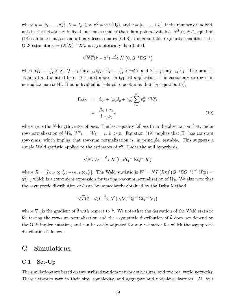
where y = [y1, . . . , yN ], X = IN ⊗ x, π0 = vec (Π′0), and v = [v1, . . . , vN ]. If the number of individ-uals in the network N is fixed and much smaller than data points available, N2 � NT , equation(18) can be estimated via ordinary least squares (OLS). Under suitable regularity conditions, theOLS estimator π = (X ′X)−1X ′y is asymptotically distributed,

√NT (π − π0)

d−→ N(0, Q−1ΣQ−1

)where QT ≡ 1

NTX ′X, Q ≡ p limT→∞QT , ΣT ≡ 1

NTX ′vv′X and Σ ≡ p limT→∞ΣT . The proof is

standard and omitted here. As noted above, in typical applications it is customary to row-sumnormalize matrix W . If no individual is isolated, one obtains that, by equation (5),

Π0ιN = β0ι+ (ρ0β0 + γ0)∞∑k=1

ρk−10 W k

0 ι

=β0 + γ0

1− ρ0

ι (19)

where ιN is the N -length vector of ones. The last equality follows from the observation that, underrow-normalization of W0, W kι = Wι = ι, k > 0. Equation (19) implies that Π0 has constantrow-sums, which implies that row-sum normalization is, in principle, testable. This suggests asimple Wald statistic applied to the estimates of π0. Under the null hypothesis,

√NTRπ

d−→ N(0, RQ−1ΣQ−1R′

)where R = [IN−1 ⊗ ι′N ;−ιN−1 ⊗ ι′N ]. The Wald statistic is W = NT (Rπ)′ (Q−1ΣQ−1)

−1(Rπ) ∼

χ2N−1 which is a convenient expression for testing row-sum normalization of W0. We also note that

the asymptotic distribution of θ can be immediately obtained by the Delta Method,

√T (θ − θ0)

d−→ N(0,∇′−1

θ Q−1ΣQ−1∇θ

)where ∇θ is the gradient of θ with respect to π. We note that the derivation of the Wald statisticfor testing the row-sum normalization and the asymptotic distribution of θ does not depend onthe OLS implementation, and can be easily adjusted for any estimator for which the asymptoticdistribution is known.

C Simulations

C.1 Set-Up

The simulations are based on two stylized random network structures, and two real world networks.These networks vary in their size, complexity, and aggregate and node-level features. All four

49

networks are also sparse. The two stylized networks considered are:

(i) Erdos-Renyi network: we randomly pick exactly one element in each row of W0 and set thatelement to 1. This is a random graph with in-degree equal to 1 for every individual (Erdosand Renyi, 1960). Such a network could be observed in practice if connections are formedindependently of one another. With N = 30, the resulting density of links is 3.45%.

(ii) Political party network: there are two parties, each with a party leader. The leader directlyaffects the behavior of half the party members. We assume that one party has twice thenumber of members as the other. More specifically, we assume individuals i = 1, . . . , N

3are

affiliated to Party A and are led by individual 1; individuals i = N3

+ 1, . . . , N are affiliatedto Party B and are led by individual N

3+1. This difference in party size allows us to evaluate

our ability to recover and identify central leaders, even in the smaller party. To test theprocedure further, we add one random link per row to represent ties that are not determinedby links to the Party leader. We simulate this network for various choices of N . If N is nota multiple of three, we round N

3to the nearest integer. With N = 30, this network has a

density of 5.17%.

(iii) Coleman’s (1964) high school friendship network survey: in 1957/8, students in a small highschool in Illinois were asked to name, “fellows that they go around with most often.” A linkwas considered if the student nominated a peer in either survey wave. The full network hasN = 73 nodes, of which 70 are non-isolated and so have at least one link to another student.On average, students named just over five friendship peers. This network has density 7.58%.Furthermore, the in-degree distribution shows that most individuals received a small numberof links, while a small number received many peer nominations.

(iv) Banerjee et al.’s (2013) village network survey: these authors conducted a census of house-holds in 75 villages in rural Karnataka, India, and survey questions include several aboutrelationships with other households in the village. To begin with, we use social ties basedon family relations (later examining insurance networks). We focus on village 10 that iscomprised of N = 77 households, and so similar in size to network (iii). In this village thereare 65 non-isolated households, with at least one family link to another household. Thisnetwork has density 5.07%.

For the stylized networks (i) and (ii), we first assess the performance of the estimator for afixed network size, N = 30. We later show how performance varies with alternative network sizes.We simulate the real-world networks (iii) and (iv) using non-isolated nodes in each (so N = 70

and 65 respectively). As in Bramoullé et al., 2009, we exclude isolated nodes because they do notconform with row-sum normalization.

50

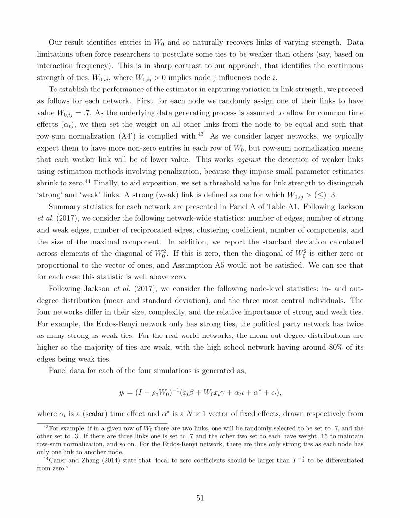
Our result identifies entries in W0 and so naturally recovers links of varying strength. Datalimitations often force researchers to postulate some ties to be weaker than others (say, based oninteraction frequency). This is in sharp contrast to our approach, that identifies the continuousstrength of ties, W0,ij, where W0,ij > 0 implies node j influences node i.

To establish the performance of the estimator in capturing variation in link strength, we proceedas follows for each network. First, for each node we randomly assign one of their links to havevalue W0,ij = .7. As the underlying data generating process is assumed to allow for common timeeffects (αt), we then set the weight on all other links from the node to be equal and such thatrow-sum normalization (A4’) is complied with.43 As we consider larger networks, we typicallyexpect them to have more non-zero entries in each row of W0, but row-sum normalization meansthat each weaker link will be of lower value. This works against the detection of weaker linksusing estimation methods involving penalization, because they impose small parameter estimatesshrink to zero.44 Finally, to aid exposition, we set a threshold value for link strength to distinguish‘strong’ and ‘weak’ links. A strong (weak) link is defined as one for which W0,ij > (≤) .3.

Summary statistics for each network are presented in Panel A of Table A1. Following Jacksonet al. (2017), we consider the following network-wide statistics: number of edges, number of strongand weak edges, number of reciprocated edges, clustering coefficient, number of components, andthe size of the maximal component. In addition, we report the standard deviation calculatedacross elements of the diagonal of W 2

0 . If this is zero, then the diagonal of W 20 is either zero or

proportional to the vector of ones, and Assumption A5 would not be satisfied. We can see thatfor each case this statistic is well above zero.

Following Jackson et al. (2017), we consider the following node-level statistics: in- and out-degree distribution (mean and standard deviation), and the three most central individuals. Thefour networks differ in their size, complexity, and the relative importance of strong and weak ties.For example, the Erdos-Renyi network only has strong ties, the political party network has twiceas many strong as weak ties. For the real world networks, the mean out-degree distributions arehigher so the majority of ties are weak, with the high school network having around 80% of itsedges being weak ties.

Panel data for each of the four simulations is generated as,

yt = (I − ρ0W0)−1(xtβ +W0xtγ + αtι+ α∗ + εt),

where αt is a (scalar) time effect and α∗ is a N × 1 vector of fixed effects, drawn respectively from43For example, if in a given row of W0 there are two links, one will be randomly selected to be set to .7, and the

other set to .3. If there are three links one is set to .7 and the other two set to each have weight .15 to maintainrow-sum normalization, and so on. For the Erdos-Renyi network, there are thus only strong ties as each node hasonly one link to another node.

44Caner and Zhang (2014) state that “local to zero coefficients should be larger than T−12 to be differentiated

from zero.”

51

N(1, 1) and N(ι, IN×N) distributions. We consider T = {5, 10, 15, 25, 50, 75, 100, 125, 150}. Thetrue parameters are set to ρ0 = .3, β0 = .4 and γ0 = .5 (thus satisfying Assumption A3). Theexogenous variable (xt) and error term (εt) are simulated as standard Gaussian, both generatedfrom N(0N , IN×N) distributions. This is similar to variance terms set in other papers, e.g., Lee(2004). We later conduct a series of robustness checks to evaluate the sensitivity of the simulationsto alternative parameters choices, and the presence of common- and individual-level shocks.

For each combination of parameters, we conduct 1, 000 simulation runs. On the initial 50

runs, we choose penalization parameters p that minimize the BIC criteria on a grid. This iscomputationally intensive because it requires running the optimization procedure described inSection 3.1 as many times as the number of points in the grid for p.45 To reduce the computationalburden, we do so only in the initial 50 runs and consider these simulation runs as a calibrationof p. For the remaining 950 iterations, the penalization parameter p is set fixed at the median pcomputed over the calibration runs. This only worsens the performance of the estimator, since asub-optimal p is chosen for the majority of the iterations.

C.2 Results

We evaluate the procedure over varying panel lengths (starting from short panels with T = 5),using the following metrics. Given our core contribution is to identify the social interactions matrix,we first examine the proportion of true zero entries in W0 estimated as zeros, and the proportionof true non-zero entries estimated as non-zeros. A global perspective of the proximity betweenthe true and estimated network can be inferred from their average absolute distance betweenelements. This is the mean absolute deviation of W and Π relative to their true values, definedas MAD(W ) = 1

N(N−1)

∑i,j,i6=j |Wij − Wij,0| and MAD(Π) = 1

N(N−1)

∑i,j,i6=j |Πij − Πij,0|. The

closer these metrics are to zero, more of the elements in the true matrix are correctly estimated.Finally, we evaluate the performance of the procedure using averaged estimates of the endogenousand exogenous social effect parameters, ρ and γ. In keeping with the estimation strategy in ourempirical application, we report ‘post-Elastic Net’ estimates obtained after having estimated thesocial interactions matrix by the Elastic Net GMM procedure. We use peers-of-peers’ covariatesfrom the estimated matrix as instrumental variables.

Each Panel in Figure A1 shows a different metric as we vary T for each simulated network.Panel A shows that for each network, the proportion of zero entries in W0 correctly estimated aszeros is above 90% even when exploiting a small number of time periods (T = 5). The proportionapproaches 100% as T grows. Panel B shows the proportion of non-zeros entries estimated asnon-zeros is also high for small T . It is above 70% from T = 5 for the Erdos-Renyi network, beingat least 85% across networks for T = 25, and increasing as T grows.

45In our simulations, we set the penalization grid to p1 = [0, .025, .05, .10], p∗1 = [0, .025, .05, .10] and p2 =[0, .025, .05, .10], resulting in 43 = 64 points per run.

52

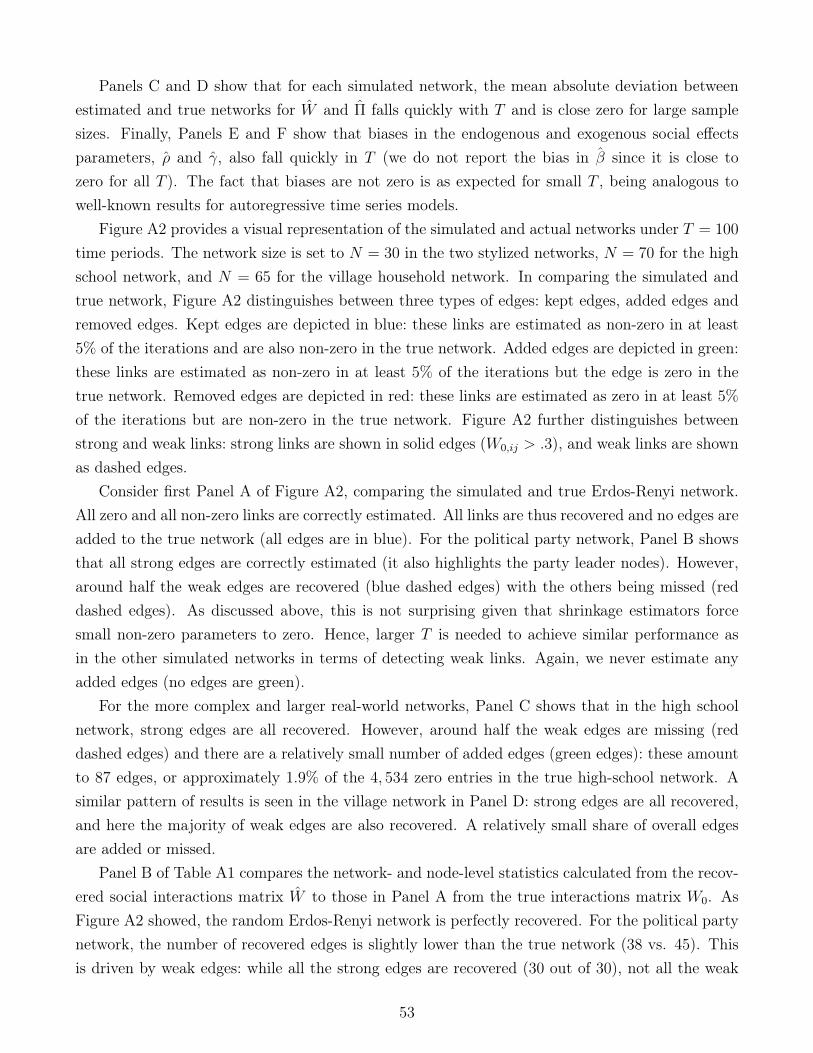
Panels C and D show that for each simulated network, the mean absolute deviation betweenestimated and true networks for W and Π falls quickly with T and is close zero for large samplesizes. Finally, Panels E and F show that biases in the endogenous and exogenous social effectsparameters, ρ and γ, also fall quickly in T (we do not report the bias in β since it is close tozero for all T ). The fact that biases are not zero is as expected for small T , being analogous towell-known results for autoregressive time series models.

Figure A2 provides a visual representation of the simulated and actual networks under T = 100

time periods. The network size is set to N = 30 in the two stylized networks, N = 70 for the highschool network, and N = 65 for the village household network. In comparing the simulated andtrue network, Figure A2 distinguishes between three types of edges: kept edges, added edges andremoved edges. Kept edges are depicted in blue: these links are estimated as non-zero in at least5% of the iterations and are also non-zero in the true network. Added edges are depicted in green:these links are estimated as non-zero in at least 5% of the iterations but the edge is zero in thetrue network. Removed edges are depicted in red: these links are estimated as zero in at least 5%of the iterations but are non-zero in the true network. Figure A2 further distinguishes betweenstrong and weak links: strong links are shown in solid edges (W0,ij > .3), and weak links are shownas dashed edges.

Consider first Panel A of Figure A2, comparing the simulated and true Erdos-Renyi network.All zero and all non-zero links are correctly estimated. All links are thus recovered and no edges areadded to the true network (all edges are in blue). For the political party network, Panel B showsthat all strong edges are correctly estimated (it also highlights the party leader nodes). However,around half the weak edges are recovered (blue dashed edges) with the others being missed (reddashed edges). As discussed above, this is not surprising given that shrinkage estimators forcesmall non-zero parameters to zero. Hence, larger T is needed to achieve similar performance asin the other simulated networks in terms of detecting weak links. Again, we never estimate anyadded edges (no edges are green).

For the more complex and larger real-world networks, Panel C shows that in the high schoolnetwork, strong edges are all recovered. However, around half the weak edges are missing (reddashed edges) and there are a relatively small number of added edges (green edges): these amountto 87 edges, or approximately 1.9% of the 4, 534 zero entries in the true high-school network. Asimilar pattern of results is seen in the village network in Panel D: strong edges are all recovered,and here the majority of weak edges are also recovered. A relatively small share of overall edgesare added or missed.

Panel B of Table A1 compares the network- and node-level statistics calculated from the recov-ered social interactions matrix W to those in Panel A from the true interactions matrix W0. AsFigure A2 showed, the random Erdos-Renyi network is perfectly recovered. For the political partynetwork, the number of recovered edges is slightly lower than the true network (38 vs. 45). Thisis driven by weak edges: while all the strong edges are recovered (30 out of 30), not all the weak

53

ones are (8 vs. 15). On node-level statistics, the mean of the in- and out-degree distributions areslightly lower in the recovered network, the clustering coefficient is exactly recovered, and all threenodes with the highest out-degree are correctly captured (nodes 1, 11 and 28), that includes bothparty leaders (individuals 1 and 11).

Performance in the two real world networks is also encouraging. In the high school network,all strong edges are correctly recovered, as are the majority of weak edges. However, as alreadynoted in Figure A2, because weak edges are not well estimated in the high school network, theaverage in- and out- degrees are smaller in the recovered network relative to the true network. Werecover two out of the three individuals with the highest out-degree (nodes 21 and 69). Finally,in the village network, all strong edges are recovered, the majority of weak edges are recovered,the clustering coefficients are similar across recovered and true networks (.134 vs. .141) and werecover two out of the three households with the highest out-degree (nodes 16, 35, and 57).

C.3 Robustness

Table A2 presents results for the recovered stylized networks under varying network sizes, N =

{15, 30, 50}. Differences between the true and estimated networks are fairly constant as N in-creases: even for small N = 15 a large proportion of zeros and non-zeros are correctly estimated.In all cases, biases in ρ and γ decrease with larger T . We also conduct a counterpart robustnesscheck for one of the real work networks. More precisely, we use the savings and insurance networksbetween households in villages identified in Banerjee et al. (2013), that are generally larger thanfamily networks focused on so far. Table A3 shows descriptive statistics on this true village net-work (Panel A) and the recovered network (Panel B). Relative to the family network, the savingsand insurance network has many more edges, a greater proportion of weak edges, is less clustered,with nodes having a higher degree distribution. Despite these differences, the recovered networkretains good accuracy on many dimensions: 78% of all edges are recovered, the recovered clusteringcoefficient is .058 (relative to an actual coefficient of .073) and the three nodes with the highestout-degree are all still identified.

Table A4 conducts robustness checks on the sensitivity of the estimates to parameters choices.We consider true parameters ρ0 = {.1, .3, .7, .9}, γ0 = {.3, .7}, β0 = {.0, .8}. We also introduce acommon shock in the disturbance variance-covariance matrix by varying q in,

εt ∼ N

0,

1 q · · · q

q 1 · · · q...

... . . . ...q q · · · 1

where we consider q = {.3, .5, .8, 1}. We find the procedure to be robust to the true values ofρ0, β0, γ0, and q. For β0 = 0, performance is slightly worse. This is expected as the exogenous

54

variation from xt no longer affects yt directly.We next probe the procedure by richening up the structure of shocks across nodes. First, we

introduce a common shock correlated with covariates xt. To do so, we take xt from a Gaussiandistribution with mean 0.5αtι and, as before, variance 1. Second, we implement a version wherethe shock is constant over time but varies at the individual level. In this case, the mean of xt isgiven by 0.5α∗. Third, we implement a version mixing the two types of shocks, with the mean ofxt given by 0.5α∗+0.5αtι. In each case, we simulate based on the Erdos-Renyi network as the trueW0. The results are shown in Figure A3: this shows that for each of the six performance metricsconsidered, the procedure is highly robust to these richer structures of shocks across individualsand time periods.

The final robustness check demonstrates the gains from using the Adaptive Elastic Net GMMestimator over alternative estimators. Table A5 shows simulation results using Adaptive Lassoestimates of the interaction matrix Π0, so estimating and penalizing the reduced-form. The Adap-tive Lasso estimator performs relatively worse: the mean absolute deviation between W and W0 isoften two to three times larger than the corresponding Adaptive Elastic Net estimates. AppendixTable A6 then shows the performance of the procedure based on OLS estimates of Π0. Given OLSrequires m� NT , we use a time dimension ten times larger, T = {500, 1000, 1500}, and still finda deterioration in performance compared to the Adaptive Elastic Net GMM estimator.

Taken together, these robustness checks suggest the Adaptive Elastic Net GMM estimator ispreferred over Adaptive Lasso and OLS estimators. This procedure does well in recovering truenetwork structures, and a fortiori, network- and node-level statistics. It does so in networks thatvary in size and complexity, and as the underlying social interactions model varies in the strengthof endogenous and exogenous social effects, and the structure of shocks.

D Application: Counterfactuals

We consider a scenario in which California exogenously increases the change in its taxes per capita,so ∆τ it corresponds to an increase of 10%. We measure the differential change in equilibrium statetaxes in state j under the two network structures using the following statistic:

Υj = log(∆τ jt|Wecon)− log(∆τ jt|Wgeo), (20)

so that positive (negative) values imply taxes being higher (or lower) under Wecon than Wgeo.46

Figure A4 graphs Υj for each mainland US state (including for California itself, the origin ofthe shock). A wide discrepancy between the equilibrium state tax rates predicted under Wecon

relative to Wgeo: across states Υj varies from −3.03 to 9.61. Only in one state is Υj close to46We calculate the counterfactual at ρ2SLS = .608, the endogenous effect parameter estimated in our preferred

specification, Column 7 of Table 2.

55

zero. Table A9 summarizes the general equilibrium effects under both structures. We see thataverage tax rate increases are 74% higher under Wecon. The dispersion of tax rates across statesalso increases dramatically under Wecon. Finally, assuming interactions across states are basedsolely on geographic neighbors, we miss the fact that many states will have relatively small taxincreases.

56

Table1:G

eographicNeighbors

Dependentvariable:C

hangeinpercapita

incomeand

corporatetaxes

Coefficientestim

ates,standarderrors

inparentheses

(1)OLS

(2)2SLS(3)O

LS(4)2SLS

Geographic

Neighbors'Tax

Change

(t-[t-2]).375***

.868***.271***

.642***

(.120)(.273)

(.075)(.152)

Period1962-1988

1962-19881962-2015

1962-2015

FirstStage(F-stat)

6.26727.320

Controls

YesYes

YesYes

Stateand

YearFixedEffects

YesYes

YesYes

Observations

1,2961,248

2,5922,544

ExtendedSam

pleBesley

andCase

(1995)Sample

Notes:

***denotes

significanceat1%,**at5%,and

*at10%

.Inallspecifications,

apair

ofstates

areconsidered

neighborsifthey

shareageographic

border.The

sample

covers48

mainland

USstates.

InColum

ns1and

2the

sample

runsfrom

1962to1988

(asinBesley

andCase

(1995)).InColum

ns3and

4the

sample

isextended

torun

from1962

to2015.The

dependentvariableisthe

changeinstate

i'stotaltaxes

percapitainyeart.O

LSregressions

estimates

areshow

ninColum

ns1

and3.Colum

ns2and

4show

2SLS

regressionswhere

eachgeographic

neighbors'taxchange

isinstrum

entedbylagged

neighbor'sstate

incomeper

capitaand

unemploym

entrate.Atthe

footofColum

ns2and

4wereportthe

p-valueonthe

F-statisticfrom

thefirststage

ofthenullhypothesis

thatinstruments

arejointly

equaltozero.A

llregressionscontrolforstate

i’sincom

epercapita

in1982

USdollars,state

i’sunem

ploymentrate,the

proportionofyoung

(aged5-17)and

elderly(aged

65+)instate

i’spopulation,and

thestate

governor'sage.A

llspecificationsinclude

stateand

timefixed

effects.Withthe

exceptionofgovernor's

age,allvariablesare

differencedbetw

eenperiod

tandperiod

t-2.Robuststandard

errorsare

reportedinparentheses.

Table2:Econom

icNeighbors

Dependentvariable:C

hangeinpercapita

incomeand

corporatetaxes

Coefficientestim

ates,standarderrors

inparentheses

(1)Initial(2)O

LS(3)2SLS:IVs

areCharacteristics

ofNeighbors

(4)Initial(5)O

LS(6)2SLS:IVs

areCharacteristics

ofNeighbors

(7)2SLS:IVsare

Characteristics

ofNeighbors-ofNeighbors

EconomicNeighbors'Tax

Change

(t-[t-2]).886

.378***.641***

.645.145**

.332*.608***

(.061)(.060)

(.072)(.199)

(.220)

PeriodFirstStage

(F-stat)19.353

9.57110.480

Controls

YesYes

YesYes

YesYes

Yes

Stateand

YearFixedEffects

YesYes

YesYes

YesYes

Yes

Observations

2,9522,952

2,5442,952

2,9522,544

2,592

ExogenousSocialEffects

1962-20151962-2015

NoExogenous

SocialEffects

Notes:***

denotessignificance

at1%,**

at5%,and

*at10%

.Thesam

plecovers

48mainland

USstates

runningfrom

1962to2015.The

dependentvariableisthe

changeinstate

i'stotal

taxesper

capitainyear

t.Weallow

forexogenous

socialeffectsinColum

ns4to7.In

subsequentOLS

andIVregressions,the

economicneighbors'effectis

calculatedasthe

weighted

averageofeconom

icneighbors'variables.O

LSregressions

estimates

areshow

ninColum

n2,3

and5.C

olumn3and

6show

the2SLS

regressionwhere

eachgeographic

neighbors'taxchange

isinstrum

entedbylagged

neighbor'sstate

incomeper

capitaand

unemploym

entrate.

Colum

n7show

sa2SLS

regressionwhere

eachgeographic

neighbors'taxchange

isinstrum

entedbylagged

neighbor-of-neighbor'sstate

incomeper

capitaand

unemploym

entrate.Atthe

footofColum

ns3,6

and7wereportthe

p-valueonthe

F-statisticfrom

thefirst

stageofthe

nullhypothesisthatinstrum

entsare

jointlyequalto

zero.Allregressions

controlforstatei’sincom

epercapita

in1982

USdollars,state

i’sunem

ploymentrate,the

proportionof

young(aged

5-17)andelderly

(aged65+)in

statei’spopulation,and

thestate

governor'sage.A

llspecificationsinclude

stateand

timefixed

effects.Withthe

exceptionofgovernor's

age,allvariables

aredifferenced

between

periodtand

periodt-2.R

obuststandarderrors

arereported

inparentheses.

Table3:G

eographicVersus

EconomicNeighborNetw

orksGeographic

NeighborNetw

orkEconom

icNeighbor

Network

Num

berofEdges214

144Edges

inBoth

Netw

orks79

79Edges

inW-geo

only135

EdgesinW-econ

only65

Clustering

.1936.0259

Reciprocated

Edges100%

29.17%

out-degree3.000

(1.185)in-degree

3.000(2.073)

4.458(1.597)

Degree

Distribution

AcrossNodes

(states)

Notes:

Thiscom

paresstatistics

derivedfrom

thegeographic

network

ofUSstates

tothose

fromthe

estimated

economic

network

among

USstates.

Thenum

berofedges,

edgesinboth

networks,

edgesinW-geo

only,edges

inW-econ

onlycounts

thenum

berofedgesinthose

categories.Reciprocated

edgesisthe

frequencyofin-edges

thatarereciprocated

byout-edges

(byconstruction,

thisis100%

forgeographic

networks).

Theclustering

coefficientisthe

frequencyofthe

number

offully

connectedtriplets

overthe

totalnum

beroftriplets.

Thedegree

distributionacross

nodescounts

theaverage

numberofconnections

(standarddeviation

inparentheses):w

eshow

thisseparately

forin-degreeand

out-degree(by

construction,theseare

identicalforgeographicnetw

orks).

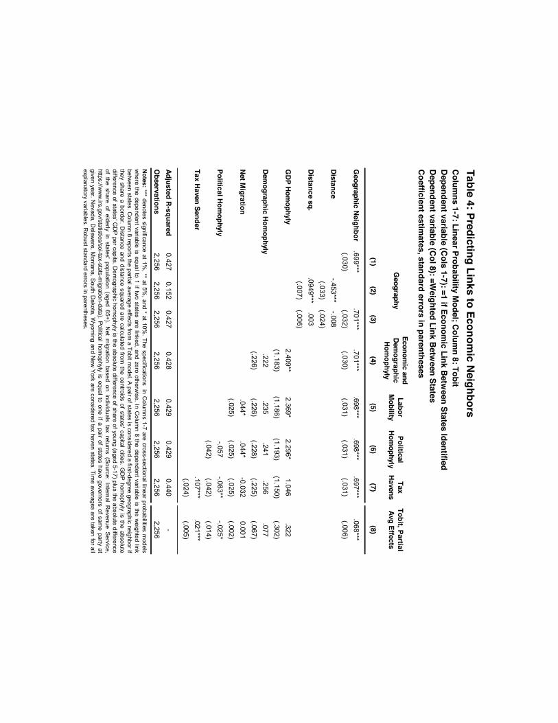
Table4:Predicting

LinkstoEconom

icNeighbors

Colum

ns1-7:LinearProbability

Model;C

olumn8:Tobit

Dependentvariable

(Cols

1-7):=1ifEconom

icLink

Betw

eenStates

IdentifiedDependentvariable

(Col8):=W

eightedLink

Betw

eenStates

Coefficientestim

ates,standarderrors

inparentheses

Economicand

Demographic

Homophyly

LaborMobility

PoliticalHom

ophylyTax

HavensTobit,PartialAvg

Effects

(1)(2)

(3)(4)

(5)(6)

(7)(8)

Geographic

Neighbor.699***

.701***.701***

.698***.698***

.697***.068***

(.030)(.032)

(.030)(.031)

(.031)(.031)

(.006)Distance

-.453***-.008

(.033)(.024)

Distancesq.

.0949***.003

(.007)(.006)

GDP

Homophyly

2.409**2.369*

2.296*1.046

.322(1.183)

(1.186)(1.193)

(1.150)(.302)

Demographic

Homophyly

.222.235

.241.256

.077(.226)

(.226)(.228)

(.225)(.067)

NetMigration

.044*.044*

-0.0320.001

(.025)(.025)

(.025)(.002)

PoliticalHomophyly

-.057-.083**

-.025*(.042)

(.042)(.014)

TaxHaven

Sender.107***

.021***(.024)

(.005)

AdjustedR-squared

0.4270.152

0.4270.428

0.4290.429

0.440-

Observations

2,2562,256

2,2562,256

2,2562,256

2,2562,256

Geography

Notes:

***denotes

significanceat1%

,**at5%

,and*at10%

.Thespecifications

inColum

ns1-7

arecross-sectionallinear

probabilitiesmodels

where

thedependentvariable

isequalto

1iftw

ostates

arelinked,and

zerootherw

ise.InColum

n8the

dependentvariableisthe

weighted

linkbetw

eenstates.C

olumn8reports

thepartialaverage

effectsfrom

aTobitm

odel.Apairofstates

isconsidered

afirst-degree

geographicneighborif

theyshare

aborder.

Distance

anddistance

squaredare

calculatedfrom

thecentroids

ofstates'capitalcities.

GDPhom

ophylyisthe

absolutedifference

ofstates'GDPpercapita.D

emographic

homophyly

isthe

absolutedifference

ofshareofyoung

(aged5-17)plus

theabsolute

differenceofthe

shareofelderly

instates'

population(aged

65+).Netmigration

basedon

individualstax

returns(Source:

InternalRevenue

Service,https://w

ww.irs.gov/statistics/soi-tax-stats-m

igration-data).Politicalhom

ophylyisequalto

oneifapair

ofstates

havegovernors

ofsam

eparty

atgiven

year.Nevada,D

elaware,M

ontana,SouthDakota,W

yoming

andNew

Yorkare

consideredtax

havenstates.Tim

eaverages

aretaken

forallexplanatory

variables.Robuststandard

errorsinparentheses.

Table5:G

ubernatorialTermLim

itsDependentvariable:Change

inpercapitalincom

eand

corporatetaxes

Coefficientestimates,standard

errorsinparentheses

IVs:CharacteristicsofNeighbors-of-Neighbors

(1)OLS

(2)2SLS(3)O

LS(4)2SLS

(5)OLS

(6)2SLS

EconomicNeighbors'tax

change(t-[t-2])

.145**.608***

.016.937*

.182**.543**

(.072)(.220)

(.105)(.534)

(.084)(.237)

PeriodFirstStage

(F-stat)10.480

2.83510.120

ControlsYes

YesYes

YesYes

Yes

Stateand

YearFixedEffects

YesYes

YesYes

YesYes

Observations

2,5922,592

640640

1,9171,917

Notes:***denotes

significanceat1%

,**at5%

,and*at10%

.Thesam

pleinColum

ns1and

2covers

48mainland

USstates

runningfrom

1962to2015.In

Colum

ns3and

4weuse

thesubsam

pleofstate-years

inwhich

thegovernorthatfaced

termlimitsinthe

subsequentgubernatorialelection.InColum

ns5and

6weuse

thesubsam

pleofstate-years

inwhich

thegovernordid

notfaceterm

limitsinthe

subsequentgubernatorialelection,andsocould

runforreelection.The

dependentvariableisthe

changeinstate

i'stotaltaxes

percapitainyear

t.Wefirst

estimate

ourprocedure

which

outputsparam

etersand

thenetw

orkofeconom

icneighbors.

Wepenalize

geographicneighbors

throughoutand

alsoallow

forexogenous

socialeffects.OLS

regressionsestim

atesare

showninColum

ns1,3

and5.C

olumns2,4

and6show

a2SLS

regressionwhere

eachgeographic

neighbors'taxchange

isinstrum

entedbylagged

neighbor-of-neighbor'sstate

incomepercapita

andunem

ploymentrate.Atthe

footofColum

ns2,4

and6wereportthe

p-valueonthe

F-statisticfrom

thefirststage

ofthenullhypothesis

thatinstruments

arejointly

equaltozero.Allregressions

controlforstate

i’sincom

eper

capitain1982

USdollars,state

i’sunem

ploymentrate,the

proportionofyoung

(aged5-17)and

elderly(aged

65+)instate

i’spopulation,and

thestate

governor'sage.Allspecifications

includestate

andtimefixed

effects.Withthe

exceptionofgovernor's

age,allvariablesare

differencedbetw

eenperiod

tandperiod

t-2.Robuststandard

errorsare

reportedinparentheses.

1962-20151962-2015

1962-2015

AllGovernors

GovernorCannotRun

forRe-election

GovernorCan

RunforRe-

election

Geographic network edgesRemoved (geographic) edges in economic networkNew edges added in economic networks

Figure 1B: Network Graph of US States, Identified Economic Neighbors

Notes: Figure 3B represents the continental United States (N=48). The economic network is derived from our preferred specification, where we penalize geographic neighbors to states, andallow for exogenous social effects. A blue edge is drawn between a pair of states if they are geographic neighbors and were estimated as connected. A red edge is drawn between a pair of statesif they are geographic neighbors but were not estimated as connected. A green edge is drawn between a pair of states if they are not geographic neighbors and were estimated connected. Theleft hand side graph just shows read and blue edges. The right hand side shows all three types of edges. State abbreviations are as used by US Post Office (http://about.usps.com/who-we-are/postal-history/state-abbreviations.pdf).

Notes: Figure 3A represents the continental US states (N=48). An edge is drawn between a pair of states if they share a geographic border. State abbreviations are as used by US Post Office(http://about.usps.com/who-we-are/postal-history/state-abbreviations.pdf).

Figure 1A: Network Graph of US States, Geographic Neighbors

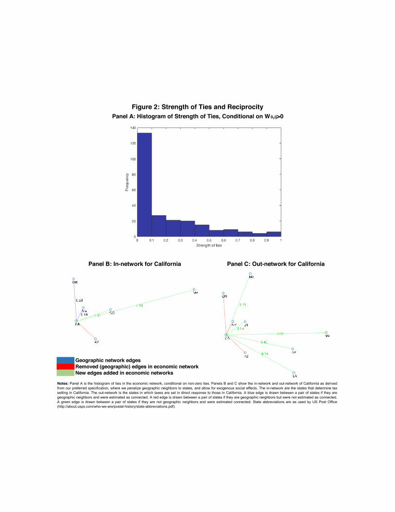
Geographic network edgesRemoved (geographic) edges in economic networkNew edges added in economic networks

Panel B: In-network for California

Figure 2: Strength of Ties and Reciprocity

Panel C: Out-network for California

Panel A: Histogram of Strength of Ties, Conditional on W0,ij>0

Notes: Panel A is the histogram of ties in the economic network, conditional on non-zero ties. Panels B and C show the in-network and out-network of California as derivedfrom our preferred specification, where we penalize geographic neighbors to states, and allow for exogenous social effects. The in-network are the states that determine taxsetting in California. The out-network is the states in which taxes are set in direct response to those in California. A blue edge is drawn between a pair of states if they aregeographic neighbors and were estimated as connected. A red edge is drawn between a pair of states if they are geographic neighbors but were not estimated as connected.A green edge is drawn between a pair of states if they are not geographic neighbors and were estimated connected. State abbreviations are as used by US Post Office(http://about.usps.com/who-we-are/postal-history/state-abbreviations.pdf).

Figure3:In-and

Out-degree

DistributionPanelA:In-degree

distributionPanelB:O

ut-degreedistribution

Notes:In-degreedistribution

(PanelA

)andout-degree

distribution(PanelB

).Distribution

calculatedfrom

geographicneighbors'netw

ork(W-geo)in

blue.Distribution

calculatedfrom

economicneighbor's

network

in(W-econ)in

red.State

abbreviationsare

asused

byUSPostO

ffice(http://about.usps.com

/who-w

e-are/postal-history/state-abbreviations.pdf).

A. % of zeros B. % of non-zeros

C. Mean Absolute Deviation of D. Mean Absolute Deviation of

E. Endogenous Social Effect, F. Exogenous Social Effect

Notes: These simulation results are based on the Banerjee et al. (2013) village network, using the Adaptive Elastic Net GMMalgorithm, with penalization parameters chosen by BIC, under various assumptions about knowledge of the true network andtime periods T=25, 50, 100, 125 and 150. The “Village" case refers to the simulation implemented without knowledge about thetrue network. "Village (top 3)" refers to the case where all connections of the three households with highest out-degrees areassumed to be known. "Village (top 5)" and "Village (top 103)" are analogously defined. In all cases, 1000 Monte Carloiterations were performed. The true parameters are rho-0=.3, beta-0=.4 and gamma-0=.5. In Panel A, the % of zeroes refers tothe proportion of true zero elements in the social interaction matrix that are estimated as smaller than .05. In Panel B, the % ofnon-zeros refers to the proportion of true elements greater than .3 in the social interaction matrix that are estimated as non-zeros. In Panels C and D, the Mean Absolute Deviations are the mean absolute error of the estimated network compared to thetrue network for the social interaction matrix W and the reduced form matrix respectively. In Panels E and F, the true parametervalues are marked in the horizontal red lines. The recovered parameter are the estimated parameters averaged acrossiterations. All specifications include time and node fixed effects.

Figure 4: Simulation Results, Adaptive Elastic Net GMMPartial Knowledge of W0

Π

ොߩ ොߛ

T=25 50 75 100 125 1500.9

0.91

0.92

0.93

0.94

0.95

0.96

0.97

0.98

0.99

1

T=25 50 75 100 125 1500

0.02

0.04

0.06

0.08

0.1

0.12

T=25 50 75 100 125 1500

0.1

0.2

0.3

0.4

0.5

0.6

0.7

0.8

0.9

1

T=25 50 75 100 125 1500.9

0.91

0.92

0.93

0.94

0.95

0.96

0.97

0.98

0.99

1

T=25 50 75 100 125 1500

0.02

0.04

0.06

0.08

0.1

0.12

T=25 50 75 100 125 1500

0.1

0.2

0.3

0.4

0.5

0.6

0.7

0.8

0.9

1

Panel B: Econ Network, 1989-2015 subsample

Panel C: Geographic Versus Economic Neighbor NetworksGeographicNeighborNetwork

Economic NeighborNetwork (Full Sample)

Economic NeighborNetwork (1962-1988)

Economic NeighborNetwork (1989-2015)

Number of Edges 214 144 197 185Edges in both W-geo and W-econ 79 108 86Edges in W-econ only 65 89 99Edges in W-geo only 135 106 128Clustering .1936 .0259 .0389 .0394Reciprocated Edges 100% 29.17% 35.53% 23.78%

out-degree 3.000 (1.185) 4.104 (1.704) 3.854 (1.473)in-degree 3.000 (2.073) 4.104 (2.707) 3.854 (2.518)

Notes: This compares statistics derived from the geographic network of US states to those from the estimated economic network among US states, for the three samples ("Full Sample", 1962-2015; 1962-1988; 1989-2015). The number of edges, edges in both networks, edges in W-geo only, edges in W-econ only counts the number of edges in those categories. Numbers are relativeto the W-geo network in the first column. Reciprocated edges is the frequency of in-edges that are reciprocated by out-edges (by construction, this is 100% for geographic networks). Theclustering coefficient is the frequency of the number of fully connected triplets over the total number of triplets. The degree distribution across nodes counts the average number of connections(standard deviation in parentheses): we show this separately for in-degree and out-degree (by construction, these are identical for geographic networks).

Panel A: Econ Network, 1962-1988 subsampleFigure 5: Network Graph of US States, Identified Economic Neighbors by Subsamples

Notes: Panels A and B represents the continental United States (N=48). Panel A is estimated withe 1962-1988 subsample. Panel B is estimated with the 1989-2015 subsample. The economicnetwork is derived from our preferred specification, where we penalize geographic neighbors to states, and allow for exogenous social effects. A blue edge is drawn between a pair of states if theyare geographic neighbors and were estimated as connected. A red edge is drawn between a pair of states if they are geographic neighbors but were not estimated as connected. A green edge isdrawn between a pair of states if they are not geographic neighbors and were estimated connected. The left hand side graph just shows read and blue edges. The right hand side shows all threetypes of edges. State abbreviations are as used by US Post Office (http://about.usps.com/who-we-are/postal-history/state-abbreviations.pdf).

Degree Distribution Across Nodes (states)

4.458 (1.597)

Erdos-Renyi Political Party High school VillageColeman (1964) Banerjee et al. (2013)

Number of nodes 30 30 70 65

(a) Network-wide statistics

Number of edges 30 45 366 240Number of strong edges 30 30 70 65Number of weak edges 0 15 296 175Number of reciprocated edges 2 2 184 240Clustering coefficient - .000 .120 .141Number of components 12 11 3 3Size of maximal component 10 16 68 51Standard deviation of thediagonal of squared W

(b) Node-level statistics

In-degree distribution 1.00 (0.00) 1.50 (.509) 5.23 (2.04) 3.69 (2.35)Out-degree distribution 1.00 (1.05) 1.50 (2.49) 5.23 (3.64) 3.69 (2.35)Nodes with highest out-degree { 7, 11, 26 } { 1, 11 , 28 } { 21, 22, 69 } { 16, 35, 57 }

(a) Network-wide statistics

Number of edges 30 38 210 194Number of strong edges 30 30 70 68Number of weak edges 0 8 140 126Number of reciprocated edges 2 2 184 170Clustering coefficient - .000 .162 .134Number of components 12 11 1 4Size of maximal component 10 14 70 48

(b) Node-level statistics

In-degree distribution 1.00 (0.00) 1.27 (.450) 3.00 (1.18) 2.99 (1.29)Out-degree distribution 1.00 (1.05) 1.27 (1.76) 3.00 (1.02) 2.99 (1.15)Nodes with highest out-degree { 7, 11, 26 } { 1, 11, 28 } { 21, 48, 69 } { 16, 35, 57 }

A. True Networks

Table A1: True and Recovered Networks

Notes: Panel A refers to the true networks. Panel B refers to the recovered networks. In each Panel, the summary statistics are divided intonetwork-wide and node-level statistics. Strong edges are defined as those with strength greater than or equal to .3. For the in-degree and out-degree distribution, the mean is shown and the standard deviation is in parentheses. The nodes with the highest out-degree are those with thegreatest influence on others, and are calculated as the column-sum of the social interaction matrix. The recovered networks statistic are calculatedover the average network across simulations with T=100.

.254 .254 .167 .239

B. Recovered Networks

TableA2:Sim

ulationResults,Adaptive

ElasticNetG

MM,Alternative

Netw

orkSizes

T=50100

150T=50

100150

T=50100

150T=50

100150

T=50100

150T=50

100150

%True

Zeroes.954

.976.973

.957.992

.997.947

.965.979

.950.977

.979.943

.978.989

.943.961

.976

(.033)(.031)

(.031)(.009)

(.004)(.002)

(.007)(.006)

(.005)(.031)

(.025)(.024)

(.009)(.006)

(.005)(.007)

(.006)(.006)

%True

Non-Zeroes

.899.919

.924.958

.960.962

.977.978

.977.914

.925.932

.930.954

.960.970

.977.977

(.051)(.032)

(.026)(.017)

(.016)(.011)

(.007)(.007)

(.008)(.038)

(.022)(.009)

(.037)(.023)

(.016)(.015)

(.009)(.007)

.021.007

.004.017

.003.001

.020.011

.006.032

.019.017

.028.014

.010.023

.014.009

(.014)(.011)

(.008)(.004)

(.001)(.001)

(.002)(.001)

(.001)(.011)

(.007)(.004)

(.004)(.002)

(.002)(.002)

(.001)(.001)

.025.012

.009.020

.004.003

.054.016

.007.034

.021.019

.028.014

.012.065

.019.009

(.012)(.008)

(.006)(.004)

(.002)(.001)

(.018)(.004)

(.002)(.009)

(.006)(.003)

(.004)(.002)

(.001)(.028)

(.004)(.001)

.262.270

.276.286

.286.283

.667.398

.270.235

.245.241

.209.228

.223.700

.383.242

(.069)(.044)

(.038)(.079)

(.026)(.022)

(.079)(.050)

(.050)(.078)

(.049)(.038)

(.084)(.035)

(.029)(.100)

(.069)(.051)

.403.399

.400.405

.400.400

.380.399

.401.405

.400.397

.404.399

.398.380

.400.401

(.039)(.028)

(.022)(.028)

(.018)(.015)

(.025)(.015)

(.012)(.040)

(.028)(.022)

(.029)(.019)

(.015)(.024)

(.015)(.012)

.577.521

.507.670

.516.498

.748.686

.595.550

.481.459

.669.501

.463.686

.666.566

(.094)(.059)

(.046)(.054)

(.022)(.018)

(.118)(.056)

(.028)(.093)

(.060)(.050)

(.060)(.027)

(.021)(.128)

(.063)(.032)

Notes:These

simulation

resultsare

basedonthe

Adaptive

Elastic

NetG

MMalgorithm

,withpenalization

parameters

chosenbyBIC,undervarious

truenetw

orks,network

sizesand

timeperiods

T=50,100and

150.Inallcases,1000

Monte

Carlo

iterationswere

performed.The

trueparam

etersare

rho-0=.3,beta-0=.4and

gamma-0=.5.The

%oftrue

zeroesrefers

tothe

proportionoftrue

zeroelem

entsinthe

socialinteractionmatrix

thatareestim

atedassmallerthan

.05.The%oftrue

non-zeroesrefers

tothe

proportionoftrue

elements

greaterthan

.3inthe

socialinteractionmatrix

thatareestim

atedasnon-zeros.The

Mean

Absolute

Deviations

arethe

mean

absoluteerror

oftheestim

atednetw

orkcom

paredtothe

truenetw

orkfor

thesocial

interactionmatrix

Wand

thereduced

formmatrix

respectively.The

recoveredparam

eterare

theestim

atedparam

etersaveraged

acrossiterations.

All

specificationsinclude

timeand

nodefixed

effects.Standard

errorsacross

iterationsare

inparentheses.

N=15

N=30

N=50

A.Erdos-Renyi

B.Politicalparty

N=15

N=30

N=50

ࢰ

ෝࢼ ࢽ ෝ

Table A3: True and Recovered Village NetworksVillage VillageFamily Savings and Insurance

Banerjee et al. (2013) Banerjee et al. (2013)

Number of nodes 65 65

(a) Network-wide statistics

Number of edges 240 343Number of strong edges 65 47Number of weak edges 175 296Number of reciprocated edges 240 340Clustering coefficient .141 .073Number of components 3 6Size of maximal component 51 62Standard deviation of thediagonal of squared W

(b) Node-level statistics

In-degree distribution 3.69 (2.35) 4.90 (3.42)Out-degree distribution 3.69 (2.35) 4.90 (3.43)Nodes with highest out-degree { 16, 35, 57 } { 16, 35, 55 }

(a) Network-wide statistics

Number of edges 194 269Number of strong edges 68 65Number of weak edges 126 204Number of reciprocated edges 170 250Clustering coefficient .134 .058Number of components 4 4Size of maximal component 48 62

(b) Node-level statistics

In-degree distribution 2.99 (1.29) 3.84 (1.90)Out-degree distribution 2.99 (1.15) 3.84 (1.98)Nodes with highest out-degree { 16, 35, 57 } { 16, 35, 55 }

.159

Notes: Panel A refers to the true networks. Panel B refers to the recovered networks. In each Panel, thesummary statistics are divided into network-wide and node-level statistics. Strong edges are defined as thosewith strength greater than or equal to .3. For the in-degree and out-degree distribution, the mean is shown andthe standard deviation is in parentheses. The nodes with the highest out-degree are those with the greatestinfluence on others, and are calculated as the column-sum of the social interaction matrix. The recoverednetworks statistic are calculated over the average network across simulations with T=100.

.239

A. True Networks

B. Recovered Networks

TableA4:Sim

ulationResults,Adaptive

ElasticNetG

MM,Alternative

Parameters

.1.5

.7.9

.0.8

.3.7

.3.5

.81.0

.1.5

.7.9

.0.8

.3.7

.3.5

.81.0

%True

Zeroes.986

.994.991

.979.986

.987.974

.997.996

.997.997

.997.971

.983.982

.966.978

.977.959

.986.985

.992.996

.997

(.005)(.004)

(.004)(.005)

(.005)(.007)

(.006)(.002)

(.002)(.003)

(.002)(.002)

(.008)(.005)

(.006)(.007)

(.008)(.007)

(.007)(.005)

(.004)(.004)

(.004)(.003)

%True

Non-Zeroes.951

.963.963

.956.806

.967.961

.961.963

.962.961

.959.772

.813.836

.864.469

.856.741

.834.803

.808.816

.832

(.028)(.011)

(.011)(.017)

(.096).000

(.015)(.016)

(.012)(.013)

(.013)(.018)

(.045)(.036)

(.034)(.031)

(.147)(.035)

(.044)(.036)

(.037)(.035)

(.034)(.027)

.005.002

.003.007

.014.004

.011.001

.001.001

.000.000

.017.012

.012.018

.029.012

.023.010

.011.009

.008.007

(.002)(.001)

(.001)(.002)

(.005)(.002)

(.003)(.001)

(.001)(.001)

(.001)(.001)

(.003)(.002)

(.002)(.003)

(.007)(.002)

(.003)(.002)

(.002)(.001)

(.001)(.001)

.005.006

.013.077

.013.007

.009.004

.003.003

.002.002

.011.021

.043.208

.021.017

.016.016

.013.011

.010.009

(.002)(.002)

(.005)(.051)

(.004)(.003)

(.002)(.002)

(.001)(.001)

(.001)(.001)

(.002)(.002)

(.004)(.026)

(.004)(.003)

(.002)(.002)

(.002)(.001)

(.001)(.001)

.081.487

.709.917

.318.244

.287.286

.285.285

.288.292

.046.403

.598.847

.298.171

.221.225

.224.222

.218.218

(.034)(.027)

(.025)(.012)

(.047)(.076)

(.036)(.023)

(.023)(.020)

(.017)(.009)

(.038)(.031)

(.040)(.040)

(.071)(.067)

(.048)(.030)

(.030)(.028)

(.025)(.018)

.401.399

.397.364

(.008).801

.402.399

.401.400

.400.400

.400.399

.398.380

-.015.801

.402.400

.399.398

.398.398

(.018)(.019)

(.019)(.023)

(.025)(.018)

(.019)(.019)

(.016)(.012)

(.009)(.001)

(.019)(.020)

(.020)(.026)

(.029)(.020)

(.020)(.019)

(.016)(.014)

(.009)(.003)

.532.512

.517.509

.432.552

.376.698

.503.495

.493.492

.519.489

.488.469

.305.548

.391.638

.474.454

.440.431

(.023)(.022)

(.024)(.028)

(.070)(.033)

(.027)(.021)

(.018)(.015)

(.012)(.007)

(.030)(.027)

(.031)(.050)

(.117)(.038)

(.036)(.025)

(.023)(.019)

(.015)(.010)

B.Politicalparty

Notes:These

simulation

resultsare

basedonthe

Adaptive

Elastic

NetG

MMalgorithm

,withpenalization

parameters

chosenbyBIC,undervarious

truenetw

orks,network

sizes,timeperiods

T=100and

parametervalues.In

allcases,1000

Monte

Carlo

iterationswere

performed.The

%oftrue

zeroesrefers

tothe

proportionoftrue

zeroelem

entsinthe

socialinteractionmatrix

thatareestim

atedassmallerthan

.05.The%oftrue

non-zeroesrefers

tothe

proportionof

trueelem

entsgreaterthan

.3inthe

socialinteractionmatrix

thatareestim

atedasnon-zeros.The

Mean

Absolute

Deviations

arethe

mean

absoluteerrorofthe

estimated

network

compared

tothe

truenetw

orkforthe

socialinteractionmatrix

Wand

thereduced

formmatrix

respectively.Therecovered

parameter

arethe

estimated

parameters

averagedacross

iterations.Allspecifications

includetimeand

nodefixed

effects.Standard

errorsacross

iterationsare

inparentheses.

qq

A.Erdos-Renyi

ࢼ

ࢽ

ࢰ

ෝࢼ ࢽෝ

ࢼ

ࢽ

T=50100

150T=50

100150

T=50100

150T=50

100150

T=50100

150T=50

100150

%True

Zeroes.728

.798.842

.737.848

.878.845

.846.913

.730.799

.840.737

.849.880

.846.846

.921

(.023)(.024)

(.022)(.012)

(.008)(.008)

(.005)(.006)

(.027)(.024)

(.025)(.023)

(.013)(.009)

(.009)(.006)

(.006)(.008)

%True

Non-Zeroes

.9961.000

1.000.497

1.0001.000

.494.496

.930.992

1.0001.000

.5071.000

1.000.498

.501.996

(.039)(.000)

(.000)(.096)

(.001)(.000)

(.071)(.074)

(.177)(.023)

(.002)(.000)

(.105)(.004)

(.001)(.074)

(.076)(.042)

.071.050

.039.064

.039.033

.039.039

.027.070

.050.039

.063.038

.032.039

.038.025

(.005)(.005)

(.004)(.002)

(.002)(.002)

(.000)(.002)

(.005)(.005)

(.004)(.004)

(.002)(.002)

(.002)(.000)

(.002)(.001)

.092.056

.042.084

.049.036

.071.045

.032.093

.057.044

.084.050

.036.071

.045.033

(.008)(.005)

(.004)(.005)

(.003)(.002)

(.004)(.003)

(.002)(.008)

(.005)(.003)

(.005)(.003)

(.002)(.004)

(.002)(.002)

.962.815

.535.998

.988.965

1.000.993

.995.970

.783.512

.998.993

.9791.000

.994.995

(.112)(.186)

(.231)(.040)

(.066)(.095)

(.000)(.075)

(.054)(.106)

(.199)(.236)

(.041)(.050)

(.077)(.000)

(.069)(.054)

.131.285

.330.000

.158.254

.000.000

.121.144

.292.336

.000.177

.259.000

.000.167

(.079)(.049)

(.038)(.000)

(.053)(.030)

(.000)(.000)

(.066)(.081)

(.049)(.039)

(.000)(.047)

(.030)(.000)

(.000)(.044)

.996.998

.968.000

1.000.999

.000.000

.8631.000

.995.942

.0001.000

.999.000

.000.992

(.063)(.015)

(.051)(.000)

(.000)(.007)

(.000)(.000)

(.344)(.000)

(.023)(.066)

(.000)(.000)

(.014)(.000)

(.000)(.089)

Notes:These

simulation

resultsare

basedonthe

Adaptive

Lassoalgorithm

,withpenalization

parameters

chosenbyBIC,undervarious

truenetw

orks,network

sizesand

timeperiods

T=50,100

and150.

Inallcases,

1000Monte

Carlo

iterationswere

performed.

Thetrue

parameters

arerho-0=.3,beta-0=.4

andgam

ma-0=.5.

The%oftrue

zeroesrefers

tothe

proportionoftrue

zeroelem

entsinthe

socialinteractionmatrix

thatareestim

atedassmallerthan

.05.The%oftrue

non-zeroesrefers

tothe

proportionoftrue

elements

greaterthan.3inthe

socialinteractionmatrix

thatareestim

atedasnon-zeros.The

Mean

Absolute

Deviations

arethe

mean

absoluteerrorofthe

estimated

network

compared

tothe

truenetw

orkfor

thesocialinteraction

matrix

Wand

thereduced

formmatrix

respectively.Therecovered

parameter

arethe

estimated

parameters

averagedacross

iterations.Allspecifications

includetimeand

nodefixed

effects.Standard

errorsacross

iterationsare

inparentheses.

TableA5:Sim

ulationResults,Adaptive

LassoA.Erdos-R

enyiB.Politicalparty

N=15

N=30

N=50

N=15

N=30

N=50

ࢰ

ෝࢼ ࢽ ෝ

T=5001000

1500T=500

10001500

T=5001000

1500T=500

10001500

T=5001000

1500T=500

10001500

%True

Zeroes.825

.878.911

.884.928

.958.936

.966.979

.824.882

.916.886

.932.959

.940.967

.979

(.018)(.020)

(.021)(.007)

(.007)(.006)

(.019)(.003)

(.002)(.020)

(.021)(.020)

(.007)(.007)

(.005)(.003)

(.003)(.002)

%True

Non-Zeroes

1.0001.000

1.0001.000

1.0001.000

.9771.000

1.0001.000

1.0001.000

1.0001.000

1.0001.000

1.0001.000

(.000)(.000)

(.000)(.000)

(.000)(.000)

(.107)(.000)

(.000)(.000)

(.000)(.000)

(.000)(.000)

(.000)(.000)

(.000)(.000)

.039.032

.028.031

.025.022

.025.021

.019.037

.030.025

.030.024

.021.024

.020.018

(.003)(.004)

(.004)(.001)

(.001)(.001)

(.000)(.000)

(.000)(.003)

(.003)(.003)

(.001)(.001)

(.001)(.000)

(.000)(.000)

.038.027

.022.039

.027.022

.040.027

.022.038

.027.022

.038.027

.022.039

.027.022

(.002)(.001)

(.001)(.001)

(.001)(.001)

(.001)(.000)

(.000)(.002)

(.001)(.001)

(.001)(.001)

(.001)(.001)

(.000)(.000)

.488.381

.3621.000

.981.617

1.0001.000

1.000.465

.396.382

1.000.953

.5901.000

1.0001.000

(.114)(.117)

(.108)(.000)

(.051)(.064)

(.000)(.000)

(.000)(.108)

(.104)(.074)

(.000)(.075)

(.062)(.000)

(.000)(.000)

.394.398

.399.343

.372.400

.256.350

.353.397

.401.399

.346.382

.400.280

.350.350

(.017)(.009)

(.006)(.017)

(.025)(.003)

(.064)(.002)

(.013)(.022)

(.014)(.005)

(.013)(.024)

(.000)(.029)

(.002)(.000)

.964.871

.8091.000

1.000.998

.9561.000

1.000.955

.841.769

1.0001.000

.9951.000

1.0001.000

(.046)(.079)

(.083)(.000)

(.000)(.009)

(.205)(.000)

(.000)(.053)

(.068)(.046)

(.000)(.000)

(.015)(.000)

(.000)(.000)

Notes:

Thesesim

ulationresults

arebased

onOLS

estimates,under

varioustrue

networks,netw

orksizes

andtimeperiods

T=500,1000and

1500.Inallcases,1000

Monte

Carlo

iterationswere

performed.The

trueparam

etersare

rho-0=.3,beta-0=.4and

gamma-0=.5.The

%oftrue

zeroesrefers

tothe

proportionoftrue

zeroelem

entsinthe

socialinteractionmatrix

thatareestim

atedassmallerthan

.05.The%oftrue

non-zeroesrefers

tothe

proportionoftrue

elements

greaterthan.3inthe

socialinteractionmatrix

thatareestim

atedas

non-zeros.TheMean

Absolute

Deviations

arethe

mean

absoluteerrorofthe

estimated

network

compared

tothe

truenetw

orkforthe

socialinteractionmatrix

Wand

thereduced

formmatrix

respectively.Therecovered

parameterare

theestim

atedparam

etersaveraged

acrossiterations.A

llspecificationsinclude

timeand

nodefixed

effects.Standard

errorsacross

iterationsare

inparentheses.

TableA6:Sim

ulationResults,O

LSA.Erdos-R

enyiB.Politicalparty

N=15

N=30

N=50

N=15

N=30

N=50

ࢰ

ෝࢼ ࢽ ෝ

TableA7:Sum

mary

Statistics,TaxCom

petitionApplication

Obs

Mean

SDMin

q25Median

q75Max

Statetotaltax

percapita1296

.371.266

.036.145

.300.530

1.345State

incomepercapita

12969.951

2.1304.105

8.5859.919

11.37518.808

Unem

ploymentrate

12965.885

2.2421.800

4.2005.500

7.00018.000

Proportionofyoung

1296.234

.033.160

.210.240

.260.310

Proportionofelderly

1296.106

.020.040

.090.110

.120.190

Stategovernor's

age1296

51.0887.441

33.00045.000

50.00056.000

73.000Governorterm

limitdum

my

1296.258

.438.000

.000.000

1.0001.000

Statetotaltax

percapita2688

0.9830.803

0.0360.037

0.8131.557

4.298State

incomepercapita

273613.268

4.0164.147

10.34812.960

15.87927.974

Unem

ploymentrate

26885.764

2.0261.800

4.3005.400

6.80017.800

Proportionofyoung

26880.236

0.0330.170

0.2100.230

0.2600.340

Proportionofelderly

26880.117

0.0230.050

0.1000.120

0.1300.190

Stategovernor's

age2736

53.5578.134

33.00047.000

53.00059.000

78.000Governorterm

limitdum

my

26380.249

0.4330.000

0.0000.000

0.0001.000

Notes:

Summary

statisticsofvariables

(inlevels)

usedinsubsequent

regressions.Besley

andCase

sample

runsfrom

1962to1988

andextended

sample

until2014.State

totaltaxpercapita

isthe

sumofsales,incom

eand

corporationtax

inthousands

of1982USdollars.

State

incomepercapita

inthousands

of1982USdollars.P

roportionofyoung

isthe

proportionofthe

populationbetw

een5and

17years.P

roportionofelderly

isthe

proportionofthe

populationaged

65orolder.S

tategovernor's

ageinyears.G

overnortermlimitdum

myisequalto

1ifgovernor

facesterm

limitsinthe

currentmandate.D

atasources:S

tatetotaltax

percapita,Census

ofGovernm

ents(1972,1977,1982,1987,1992-2016)

andAnnual

Survey

ofGoverm

entFinances

(allother

years);Steta

incomeper

capita,Bureau

ofEconom

icAnalysis;

Unem

ployment

rate,Bureau

ofLaborStatistics;P

roportionofyoung

(aged5-17)

andelderly

(aged65+),C

ensusPopulation

&Housing

Data;S

tategovernor's

ageand

politicalvariablesmanually

sourcedfrom

individualgovernor'swebpages

onWikipedia.

A.Besley

andCase

sample

(1962-1988)

B.Extended

sample

(1962-2014)

TableA8:Exogenous

SocialEffectsDependentvariable:C

hangeinpercapitalincom

eand

corporatetaxes

Coefficientestim

ates,standarderrors

inparentheses

(1)Initial(2)O

LS(3)2SLS:IVs

areCharacteristics

ofNeighbors

(4)2SLS:IVsare

Characteristics

ofNeighbors-ofN

eighbors

EconomicNeighbors'tax

change(t-[t-2])

.645.145**

.332*.608***

(.072)(.199)

(.220)

EconomicNeighbors'incom

epercapita

.090.098***

.091***.080***

(.011)(.012)

(.014)

EconomicNeighbors'unem

ploymentrate

37.2009.899***

11.780***13.714***

(3.443)(2.856)

(3.022)

EconomicNeighbors'population

aged5-17

1378.1376.2

478.5596.6

(399.0)(414.2)

(401.7)

EconomicNeighbors'population

aged65+

-4304.5-842.8

-769.7*-641.3

(504.3)(450.2)

(468.6)

EconomicNeighbors'governorage

-2.158-0.311

-0.293-0.263

(.281)(.285)

(.294)

PeriodFirstStage

(F-stat)9.571

10.480

Controls

YesYes

YesYes

Stateand

YearFixedEffects

YesYes

YesYes

Observations

2,9522,952

2,5442,592

1962-2015

Notes:***denotes

significanceat1%

,**at5%

,and*at10%

.Thesam

plecovers

48mainland

USstates

runningfrom

1962to2015.The

dependentvariable

isthe

changeinstate

i'stotal

taxesper

capitainyear

t.InallC

olumns,

wepenalize

geographicneighbors

inallColum

nsand

allowfor

exogenoussocialeffects.

InOLS

andIVregressions,

theeconom

icneighbors'effect

iscalculated

asthe

weighted

averageofeconom

icneighbors'

variables.OLS

regressionsestim

atesare

showninColum

n2.C

olumn3show

sthe

2SLS

regressionwhere

eachgeographic

neighbors'taxchange

isinstrum

entedby

laggedneighbor's

stateincom

eper

capitaand

unemploym

entrate.

Colum

n4show

sa2SLS

regressionwhere

eachgeographic

neighbors'taxchange

isinstrum

entedbylagged

neighbor-of-neighbor'sstate

incomepercapita

andunem

ploymentrate.A

tthefootofC

olumns3and

4wereportthe

p-valueonthe

F-statisticfrom

thefirststage

ofthenullhypothesis

thatinstruments

arejointly

equaltozero.A

llregressionscontrolfor

statei’sincom

eper

capitain1982

USdollars,

statei’sunem

ployment

rate,the

proportionofyoung

(aged5-17)

andelderly

(aged65+)

instate

i’spopulation,and

thestate

governor'sage.A

llspecificationsinclude

stateand

timefixed

effects.Withthe

exceptionofgovernor's

age,allvariablesare

differencedbetw

eenperiod

tandperiod

t-2.Robuststandard

errorsare

reportedinparentheses.

TableA9:G

eneralEquilibriumImpacts

ofCaliforniaTax

RiseGeographic

NeighborNetw

orkEconom

icNeighbor

Network

Ratio

Averagetax

increase0.0038

0.00661.74

Variancetax

increase0.0160

0.01530.96

Taxdispersion

0.00530.0141

2.66

Stateswith

taxincrease

4848

1.00States

with

taxincrease

>0.05%

1144

4.00States

with

taxincrease

>0.5%

511

2.20States

with

taxincrease

>1%

48

2.00States

with

taxincrease

>2.5%

13

3.00States

with

taxincrease

>5%

11

1.00

Notes:This

showsthe

equilibriumimpulse

responsesintaxes

setineach

stateasaresultofC

aliforniaincreasing

itstax

changeby10%

.Therho

coefficientisderived

fromour

preferredspecification

toestim

atethe

economicnetw

ork,where

wepenalize

geographicneighbors

tostates,and

allowfor

exogenoussocialeffects

(basedon

asam

pleof48

mainland

USstates

runningfrom

1962to2015).

Wecom

parethese

derivedtax

changesunder

theidentified

economicnetw

orkstructure,

relativetothat

assumed

underageographic

neighborsstructure.

ThefinalC

olumn

showsthe

ratioofthe

samestatistic

derivedundereach

network.

A. % of zeros B. % of non-zeros

C. Mean Absolute Deviation of D. Mean Absolute Deviation of

E. Endogenous Social Effect, F. Exogenous Social Effect

Notes: These simulation results are based on the Adaptive Elastic Net GMM algorithm, with penalization parameters chosenby BIC, under various true networks and time periods T=5, 10, 15, 25, 50, 100, 125 and 150. In all cases, 1000 Monte Carloiterations were performed. The true parameters are rho-0=.3, beta-0=.4 and gamma-0=.5. In Panel A, the % of zeroes refersto the proportion of true zero elements in the social interaction matrix that are estimated as smaller than .05. In Panel B, the %of non-zeros refers to the proportion of true elements greater than .3 in the social interaction matrix that are estimated as non-zeros. In Panels C and D, the Mean Absolute Deviations are the mean absolute error of the estimated network compared tothe true network for the social interaction matrix W and the reduced form matrix respectively. In Panels E and F, the trueparameter values are marked in the horizontal red lines. The recovered parameter are the estimated parameters averagedacross iterations. All specifications include time and node fixed effects.

Figure A1: Simulation Results, Adaptive Elastic Net GMM

Π

ොߩ ොߛ

T=5 10 15 25 50 75 100 125 1500.5

0.55

0.6

0.65

0.7

0.75

0.8

0.85

0.9

0.95

1

T=5 10 15 25 50 75 100 125 1500.5

0.55

0.6

0.65

0.7

0.75

0.8

0.85

0.9

0.95

1

T=5 10 15 25 50 75 100 125 1500

0.1

0.2

0.3

0.4

0.5

0.6

0.7

0.8

T=5 10 15 25 50 75 100 125 1500

0.2

0.4

0.6

0.8

1

1.2

T=5 10 15 25 50 75 100 125 1500

0.2

0.4

0.6

0.8

1

1.2

T=5 10 15 25 50 75 100 125 1500

0.1

0.2

0.3

0.4

0.5

0.6

0.7

0.8

Figure A2: Simulated and True Networks

Notes: These simulation results are based on the Elastic Net algorithm, with penalization parameters chosen by BIC, under varioustrue networks and time periods T=50, 100 and 150. In the two stylized networks (Erdos-Renyi and political party), we set N=30, andthe real world networks, the high school friendship and village network are based on N=65 and 70 non-isolated nodes respectively.Party leaders in the political party network are marked in black in Panel B. In all cases, 1,000 Monte Carlo iterations were performed.The true parameters are rho-0=.3, beta-0=.4 and gamma-0=.5. All specifications include time and node fixed effects. Kept edges aredepicted in blue: these links are estimated as non-zero in at least 5% of the iterations and are also non-zero in the true network.Added edges are depicted in green: these links are estimated as non-zero in at least 5% of the iterations but the edge is zero in thetrue network. Removed edges are depicted in red: these links are estimated as zero in at least 5% of the iterations but are non-zero inthe true network. The figures further distinguish between strong and weak links: strong links are shown in solid edges (whose strengthis greater than or equal to .3), and weak links are shown as dashed edges.

A. Erdos-Renyi B. Political Party

C. High-school D. Village

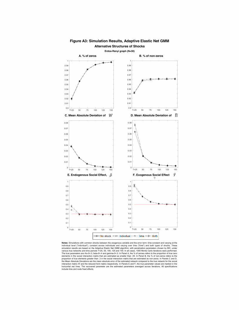
A. % of zeros B. % of non-zeros

C. Mean Absolute Deviation of D. Mean Absolute Deviation of

E. Endogenous Social Effect, F. Exogenous Social Effect

Figure A3: Simulation Results, Adaptive Elastic Net GMM

Erdos-Renyi graph (N=30)

Notes: Simulations with common shocks between the exogenous variable and the error term: time-constant and varying at theindividual level ("individual"), constant across individuals and varying over time ("time") and both types of shocks. Thesesimulation results are based on the Adaptive Elastic Net GMM algorithm, with penalization parameters chosen by BIC, undervarious true networks and time periods T=25, 50, 100, 125 and 150. In all cases, 1000 Monte Carlo iterations were performed.The true parameters are rho-0=.3, beta-0=.4 and gamma-0=.5. In Panel A, the % of zeroes refers to the proportion of true zeroelements in the social interaction matrix that are estimated as smaller than .05. In Panel B, the % of non-zeros refers to theproportion of true elements greater than .3 in the social interaction matrix that are estimated as non-zeros. In Panels C and D,the Mean Absolute Deviations are the mean absolute error of the estimated network compared to the true network for the socialinteraction matrix W and the reduced form matrix respectively. In Panels E and F, the true parameter values are marked in thehorizontal red lines. The recovered parameter are the estimated parameters averaged across iterations. All specificationsinclude time and node fixed effects.

Alternative Structures of Shocks

Π

ොߩ ොߛ

T=25 50 75 100 125 1500.9

0.91

0.92

0.93

0.94

0.95

0.96

0.97

0.98

0.99

1

T=25 50 75 100 125 1500

0.01

0.02

0.03

0.04

0.05

0.06

0.07

0.08

T=25 50 75 100 125 1500

0.1

0.2

0.3

0.4

0.5

0.6

0.7

0.8

0.9

1

T=25 50 75 100 125 1500.9

0.91

0.92

0.93

0.94

0.95

0.96

0.97

0.98

0.99

1

T=25 50 75 100 125 1500

0.01

0.02

0.03

0.04

0.05

0.06

0.07

0.08

T=25 50 75 100 125 1500

0.1

0.2

0.3

0.4

0.5

0.6

0.7

0.8

0.9

1

Positivevalues

indicatehigherequilibrium

taxesunderEconom

icneighbors

thangeographic

neighborsNegative

valuesindicate

lowequilibrium

taxesunderEconom

icneighbors

thangeographic

neighbors

FigureA4:G

eneralEquilibriumImpacts

ofCATax

Rise

ShocksState's

Reactionto10%

increaseinCA

taxes

Log(equilibriumtaxes

underW-econ)-Log(equilibrium

taxesunderW

-geo)

Notes:This

showsthe

equilibriumimpulse

responsesintaxes

setineach

stateasaresult

ofCalifornia

increasingitstax

changeby10%

.This

isas

derivedfrom

ourpreferred

specification,where

wepenalize

geographicneighbors

tostates,and

allowforexogenous

socialeffects.Wecom

parethese

derivedtax

changesunderthe

identifiedeconom

icnetw

orkstructure,relative

tothatassum

edundera

geographicneighbors

structure.Wegraph

thelog

changeinequilibrium

taxesundereconom

icneighbors,m

inusthe

logchange

inequilibrium

taxesunder

geographicneighbors.

Positive

values(red

shaded)states

indicatehigher

equilibriumtaxes

undereconom

icneighbors

thangeographic

neighbors,and

negativevalues

(blueshaded)states

indicatelowerequilibrium

taxesundereconom

icneighbors

thangeographic

neighbors.