identifying preseizure state in intracranial eeg …
TRANSCRIPT

MATHEMATICAL BIOSCIENCES doi:10.3934/mbe.2013.10.579AND ENGINEERINGVolume 10, Number 3, June 2013 pp. 579–590
IDENTIFYING PRESEIZURE STATE IN INTRACRANIAL EEG
DATA USING DIFFUSION KERNELS
Dominique Duncan
101 AKW, 51 Prospect St. New Haven, CT 06511, USA
Ronen Talmon
103 AKW, 51 Prospect St. New Haven, CT 06511, USA
Hitten P. Zaveri
716 LLCI, 15 York St. New Haven, CT 06520, USA
Ronald R. Coifman
108A AKW, 51 Prospect St. New Haven, CT 06511, USA
Abstract. The goal of this study is to identify preseizure changes in intracra-
nial EEG (icEEG). A novel approach based on the recently developed diffusion
map framework, which is considered to be one of the leading manifold learningmethods, is proposed. Diffusion mapping provides dimensionality reduction of
the data as well as pattern recognition that can be used to distinguish different
states of the patient, for example, interictal and preseizure. A new algorithm,which is an extension of diffusion maps, is developed to construct coordinates
that generate efficient geometric representations of the complex structures inthe icEEG data. In addition, this method is adapted to the icEEG data and
enables the extraction of the underlying brain activity.
The algorithm is tested on icEEG data recorded from several electrodecontacts from a patient being evaluated for possible epilepsy surgery at the
Yale-New Haven Hospital. Numerical results show that the proposed approach
provides a distinction between interictal and preseizure states.
1. Introduction. Approximately 50 million people worldwide suffer from epilepsy,including 2.7 million people in the United States, making it one of the most commonneurological disorders [7]. Seizures are successfully controlled in 64% of patients,while the remaining 36% have pharmacoresistant epilepsy [9]. Epilepsy surgery isan option for some of the patients with pharmacoresistant epilepsy if their seizurescan be localized to a focal area of the brain.
It is important to find a reliable method to predict seizures so that a patient canbe warned at least a few minutes prior to the seizure and take effective precautions.Finding an accurate predictor of seizures has become a major focus of researchduring the last few decades [5]. Seizure prediction algorithms can be used to improvedevices to control seizures. The Neuropace device, for example, which is placedwithin the skull, contains a programmable feature detector that can be employedto stimulate on detection of target features [15]. However, it is still important to
2010 Mathematics Subject Classification. 68T10, 65F15, 92B99, 92C20, 00A69.Key words and phrases. Intracranial EEG, epilepsy, seizure prediction, diffusion maps, nonlin-
ear independent component analysis.
579

580 D. DUNCAN, R. TALMON, H. P. ZAVERI AND R. R. COIFMAN
improve these feature detectors and find ways to predict seizures with sufficientsensitivity and specificity.
In our ongoing research, we have investigated various methods to analyze icEEGdata, such as coherence, mutual information, and approximate entropy [4] to an-alyze resting state icEEG activity. Seizure prediction involves a wide variety ofmethods, including linear methods, such as autoregressive models, as well as nonlin-ear methods, such as estimations of the largest Lyapunov exponent and correlation[13]. Other approaches involve the comparison of interictal and preictal epochs [1].Often the main problem in many seizure prediction studies is that the analysis isperformed on a small amount of data from few patients.
In EEG data, we assume that the measurements are controlled by underlyingprocesses that represent brain activity. We would like to recover these underlyingbrain processes to distinguish different brain states, such as interictal and preseizurestates. Diffusion maps [3] have been a useful tool in reducing the dimensionalityof the data as well as providing a measure for pattern recognition and featuredetection. Since diffusion mapping may detect abnormal behavior in the data, itcan be used to determine changes in brain states. However, diffusion maps assumeaccess to the underlying process that it aims to reveal. In EEG data, the relationshipbetween samples of the data and the underlying activity may be stochastic, and thedata are assumed to be noisy. Hence diffusion mapping is not the most suitableapproach to use with our icEEG data. A recently developed algorithm, which isan extension of diffusion maps, may be more applicable in our case [16, 17]. Thenew algorithm assumes a stochastic mapping between the underlying processes andthe measurements; the mapping is inverted and a kernel is used to recover theunderlying activity [16]. Thus, the proposed algorithm is more appropriate thandiffusion maps for our data.
In this paper, we propose an algorithm that relied on [16] for extracting theunderlying brain activity from the icEEG data. The algorithm is an extensionof diffusion maps and uses local principal components analysis (PCA). PCA isanother dimensionality reduction method. In PCA, the goal is to compute the mostmeaningful basis to re-express a large and noisy data set. This new basis can revealhidden patterns and structure in the data as well as remove the noise. An orthogonallinear transformation converts the data to a new coordinate system. The greatestvariance in the data is represented by the first coordinate or the first principalcomponent. In EEG, the data may be generated by a nonlinear combination ofsources, the underlying processes, so that more sophisticated methods are requiredto represent the data. An important difference between the proposed algorithmand PCA is the use of nonlinear locality in the extension as opposed to PCA, whichretains the linear global information of the data. For the icEEG data, we performPCA on local regions of data and then integrate the local information using a kerneland obtain a single model. We use a data-driven adapted distance between samplesof icEEG recordings to approximate the Euclidean distance between the underlyingprocesses from the noisy EEG.
2. Methods.
2.1. Intracranial EEG. 1
1Intracranial depth, subdural strip, and subdural grid electrodes were placed as required forthe patient. Subdural strip and grid electrode contacts were recessed platinum disk contacts with
2.3 mm exposed surface and 1 cm center-to-center separation (Ad-Tech, Racine, WI, U.S.A.).

IDENTIFYING PRESEIZURE STATE USING DIFFUSION KERNELS 581
Intracranial EEG (icEEG) data were collected from a patient with localizationrelated epilepsy who was undergoing presurgical evaluation at the Yale-New HavenHospital. A total of 182 electrode contacts were used during the monitoring. Theseizure onset area was located on the right occipital lobe. In this paper, we focuson the 3 electrode contacts, which overlaid the seizure onset area. Figure 1 showsthe location of the 3 electrode contacts which were studied.
Figure 1. The seizure onset area is located in the right occipitallobe. The three electrode contacts overlying the seizure onset areawhich are used in this study have been circled.
We studied 6 icEEG epochs, each of which corresponds to a seizure experiencedby the patient over the course of the icEEG monitoring. Figure 2 shows an exampleof approximately 16 minutes of icEEG data from one electrode contact that includesa seizure. The seizure start time is marked with a red line. Figure 3 shows thecorresponding spectrogram, where the horizontal axis represents time (each point isone time window). We considered the delta (0.5-4 Hz), theta (4-8 Hz), alpha (8-13Hz), beta (13-25 Hz), and gamma frequency bands (25-100 Hz).
For each case, we considered 5 minutes of data immediately preceding the seizureand 5 minutes of data from 35 minutes before the seizure, which we considered tobe the interictal state. An example is shown in Figure 4. The data were collected
Intracranial electrode contacts were located after placement using a computer program (BioImageSuite) developed at Yale University [11] and a procedure which has been described [6]. Briefly,
intracranial electrode contacts were located from a postimplantation computed tomography (CT)image. The postimplantation CT was then coregistered first with a postimplantation magneticresonance (MR) image using a linear coregistration procedure and then with a preimplantationMR image using both a linear and a nonlinear coregistration procedure. This procedure allowedus to visualize intracranial electrode contacts on preimplantation MR images. The icEEG were
collected with clinical icEEG acquisition equipment (Natus Medical Inc./Bio-Logic Systems Corp.,San Carlos, CA). The signals were sampled at 256 Hz with 16 bit A/D conversion.

582 D. DUNCAN, R. TALMON, H. P. ZAVERI AND R. R. COIFMAN
Figure 2. The icEEG from one electrode contact for approxi-mately 16 minutes including one seizure where the seizure starttime is marked with a red line. The horizontal axis represents time(in samples).
at 256 samples per second, so for each case, we analyzed 10 minutes or 153,600samples. The horizontal axis represents time (in samples). From the raw icEEGdata for this patient, it is typically unclear to determine when a seizure began untilthe actual start time of the seizure.
2.2. Data features and metric. Let y(n) be the icEEG data from a single elec-trode contact where n is the time index; we describe the following procedure fordata from merely one electrode contact for simplicity. Vectors and matrices will bedenoted in lowercase and uppercase bold, respectively. Applying the Short TimeFourier Transform (STFT) on y(n) yields
ym,k =∑n
y(n)φm,k(n), (1)
where
φm,k(n) = φ(n−mL)ej2πN k(n−mL), (2)
and m is the time frame index, k is the frequency band index, φ(n) is a Hanningwindow of length N , and L is the discrete-time shift [12]. The Hanning window isdefined as
φ(n) =1
2
(1− cos
(2πn
N − 1
)). (3)
The data are split into segments overlapped by 50%, or L = N/2, each of which arewindowed and then Fourier transformed to produce an estimate of the short-termfrequency content of the signal. Let
Sy(m,n) = |ym,n|2 (4)

IDENTIFYING PRESEIZURE STATE USING DIFFUSION KERNELS 583
Figure 3. The spectrogram of the above segment of data (ap-proximately 16 minutes) that includes a seizure, showing the delta(0.5-4 Hz), theta (4-8 Hz), alpha (8-13 Hz), beta (13-25 Hz), andgamma frequency bands (25-100 Hz). The vertical axis representsfrequency ranging from 0-100 Hz, and the horizontal axis representstime (in analysis windows).
be the squared amplitude of the STFT. We collect a few frequency bands for eachtime frame into vectors defined as
sy(m) = [..., Sy(m,n), ...]T , n ∈ K, (5)
where K is the collection of empirically relevant frequency bands. The STFT iscommonly used in time series analysis because it allows us to see the changes of thespectral composition over time. In EEG, it may enable us to identify differencesin the data closer to seizures as opposed to interictal states. We call {sy(m)} thefeature vectors.
We assume that the high dimensional features sy(m) are controlled by the lowdimensional processes that represent brain activity. The factors that describe apreseizure state are considered to be a collection of d stochastic processes θm =(θ1
m, ..., θdm), where m is the time frame index, such that each of these processes
satisfies a stochastic differential equation that can be described as
θim+1 = θim + ai(θim) + wim, (6)
where i = 1, ..., d. It is assumed that the drift terms (a1, ..., ad) are unknown and(w1
m, ..., wdm) are d independent white Gaussian noises. sy(m) is a random variable
whose statistics can be expressed as a nonlinear stochastic function of the underlyingfactors. Thus, the goal is to recover these underlying factors, which represent thepreseizure state, from the features, sy(m).
We propose the following method to reduce the dimension of the data whilekeeping the information we need to distinguish preseizure from interictal states.

584 D. DUNCAN, R. TALMON, H. P. ZAVERI AND R. R. COIFMAN
We compare feature vectors for the 5 minutes of data by calculating the STFTof the windows of data. Combining the vectors, sy(m), and plotting the outcomeshows that the feature vectors (Figure 5) do not exhibit significant variation be-tween interictal and preseizure state for the 6 separate seizure episodes. The lowerfrequency bands are most often used for detecting different states in patients usingEEG; we consider the frequency bands up to 100 Hz for our analysis. These are usedas our feature vectors for each point in time (each window of almost 4 seconds).
Given a feature vector sy(m), we compute the local covariance matrix in a timeinterval of length J :
Σm =1
J
m∑m′=m−J+1
(sy(m′)− µm)(sy(m′)− µm)T , (7)
where µm is the empirical local mean of the feature vectors in the interval.We define a nonsymmetric distance using the covariance matrices Σms:
a2Σ(m,m′) = (sy(m)− sy(m′))TΣ−1
m (sy(m)− sy(m′)) (8)
and a symmetric distance
d2Σ(m,m′) = (1/2)(a2
Σ(m,m′) + a2Σ(m′,m). (9)
The distance in (9) is termed the Mahalanobis distance, and it is shown in [14]that it approximates the Euclidean distance between the underlying factors. Thisdistance allows us in Section 2.3 to recover the underlying factors in the icEEG datavia eigendecomposition of an appropriate Laplace operator (kernel).
2.3. Kernel and embedding. Consider a collection {sy(m)} of Ns feature vec-tors. Let R be a subset of reference feature vectors of size Ns and Ns < Ns. R isobtained by selecting an arbitrary subset of measurements to enable a more efficientcomputation of the data.
A kernel is used to compare the underlying factors, whose (m,m′)th element is
Wm,m′
R = exp
{−d
2Σ(m,m′)
ε
}(10)
where ε is the kernel scale set according to the Mahalanobis distance defined above.This kernel, WR, depends on the reference set and defines the local geometries ofthe graph [3].
WR is normalized by a diagonal density matrix,
Dm,m =∑
m′∈RWm,m′
R , (11)
which enables us to view the sampling as uniform. This normalized matrix isdenoted by
WR = D−1/2WRD1/2. (12)
We can further normalize according to [8]. In order to obtain the representationof the training set, we perform an eigendecomposition to handle the nonuniformsampling of the data and acquire the eigenvalues, λj , and eigenvectors, ϕj . Theeigenvalues of the diagonal matrix are all non-negative and sorted in decreasingorder. The Laplace-Beltrami operator is given by I− WR, which shares the sameeigenvectors as WR.

IDENTIFYING PRESEIZURE STATE USING DIFFUSION KERNELS 585
In order to incorporate samples from the entire set, we form an Ns × Ns non-symmetric affinity matrix A whose (m,m′)th element is defined as
Amm′= exp
(−a
2Σ(m,m′)
ε
), (13)
where ε > 0 is the kernel scale, m′ ∈ R, and m = 1, ..., Ns.We define the diagonal matrix D and normalize A, similar to the previous nor-
malization, to form
A = D−1A. (14)
Next we define a kernel on the entire set:
W = AAT. (15)
Then we extend the eigenvectors of WR and use the diagonal density to getthe eigenvalues of W without computing the eigendecomposition of W. It can beshown by [8] that
WR = AT A. (16)
The eigenvalues and eigenvectors of WR are determined, and it is known that Wconverges to a diffusion operator [8, 17].
Proposition 3.1 from [8] states that the eigenvectors ψj of W corresponding tononzero eigenvalues λj > 0 are
ψj =1
λ1/2j
Aϕj . (17)
Using WR based on our reference set is useful, because it is smaller than thesize of the kernel based on the whole data set, and using the entire data set wouldbe computationally intensive. In practice, it is difficult to handle the icEEG data,because it is so large, so using a small matrix based on the reference set is efficient.In the algorithm, we use WR to denote the first stage with the reference featurevectors as opposed to W for the second stage. Initially, we use the reference featurevectors to perform our analysis using the kernel based on the Mahalanobis distance(9) and apply an eigendecomposition. Then we use (17) to acquire a representationof the entire set and finally define a mapping that allows us to recover the underlyingbrain activity in the icEEG data.
Based on the eigendecomposition, we define an `-dimensional embedding of eachfeature vector as the diffusion mapping:
sy(m) 7→ [λ1ψ1(m), λ2ψ2(m), ..., λ`ψ`(m)]T , (18)
and ` is related to the intrinsic dimensionality of the data for each m = 1, ..., Ns.The eigenvectors of W corresponding to the largest eigenvalues provide a parame-
trization of the features. Thus, we reduce the data from a large dimensional spaceof noisy observations to a small dimensional space, which captures the features ofpreseizure activity. In our case, we set ` = 3, so our embedding is in a 3-dimensionalspace. Our empirical example approximates heat flow on a manifold; we have highdimensional complex data, and we want to understand the intrinsic coordinates ofthe manifold. The proposed algorithm is useful for distinguishing different states(interictal and preseizure) in the icEEG data.

586 D. DUNCAN, R. TALMON, H. P. ZAVERI AND R. R. COIFMAN
3. Results. Figure 5 shows the spectrograms for the two segments of interictal andpreseizure icEEG data. The horizontal axis represents time frames, and the verticalaxis represents frequency ranging from 0-100 Hz. The spectrogram is computed byusing the Short Time Fourier Transform (STFT) in (4) with a window length of1,000 points overlapping by 50%. For EEG data, lower frequency bands reveal themost information about the state of a patient [2]. In our analysis, we consideredthe delta (0.5-4 Hz), theta (4-8 Hz), alpha (8-13 Hz), beta (13-25 Hz), and gamma(25-100 Hz) frequency bands.
After combining the resulting spectrograms for the two segments (five minutesimmediately preceding the seizure and five minutes from 35 minutes before theseizure), we apply our proposed algorithm. Figure 6 depicts a 3D scatter plot of theembedding obtained using the three leading eigenvectors from (18). Each point inthe figure represents a time frame defined in (5). The colors represent time for the10 minutes of data, with the red points corresponding to the data directly beforethe seizure. We find that this method shows a clear separation of the preseizurepoints from the interictal state points, which tend to be scattered around the origin.
Figure 4. The raw icEEG data recorded from the 3 electrode con-tacts in the seizure onset area for the interictal (left) and preseizure(right) periods; the horizontal axis represents time (in samples).
Figure 5. The spectrograms from the interictal (left) and pre-seizure (right) periods; the vertical axis represents frequency rang-ing from 0-100 Hz, and the horizontal axis represents time (in anal-ysis windows).

IDENTIFYING PRESEIZURE STATE USING DIFFUSION KERNELS 587
Figure 6. The embedding using 3 eigenvectors; the colors repre-sent time, with the red points closest to seizure onset.
From the three dimensional plot, it is quite evident that there is a clear separationbetween the points in the preseizure state and the points in the interictal state. Thered points on the graph are the points closest in time to the seizure onset, and theyare separated from the rest of the cloud of points that are near the origin. For thedata analysis of this patient, we see that for each of the times prior to the seizureoccurrences, there is no apparent difference between the interictal states and thepreseizure states in the raw data or in the spectrograms of the data. On the otherhand, there is a clear separation between the two states from the embeddings thatarise from an application of our method. This experiment was repeated for allsix seizures that the patient experienced while being monitored, and we obtainedsimilar and consistent results.
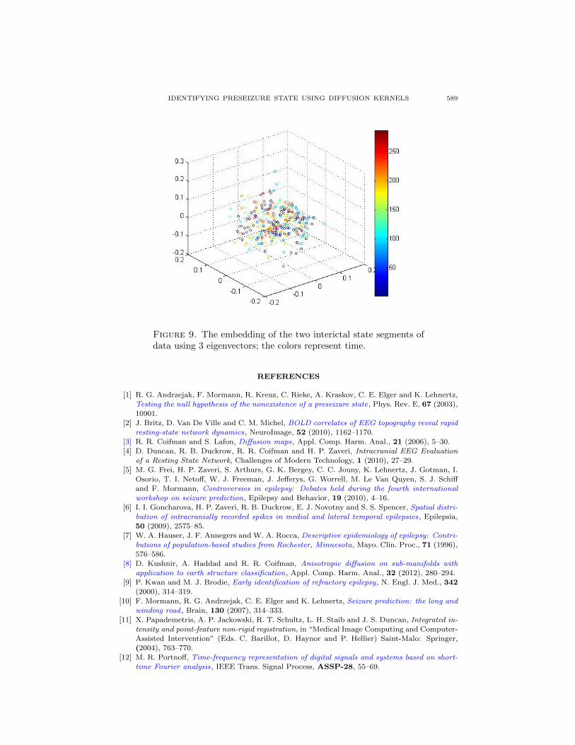
To verify that the separation did not occur from merely the time separation ofthe two data segments, two separate time segments of interictal state data werecompared, as seen in Figure 7. In the previous case, we use one segment of pre-seizure data compared to one segment of interictal data from 30 minutes before thatpreseizure segment. We compare that segment of interictal data to another segmentof interictal data from 30 minutes prior to it and also computed the spectrogramsusing (4), as seen in Figure 8. It was seen that there was no discernible separationof these two interictal state data segments using (18) in the embedding in Figure9. An analysis of other interictal state and preseizure data for this patient showedthe same type of separation as shown in Figure 6, whereas other embeddings usingtwo separate interictal periods showed no separation.
4. Discussion. Based on this initial study, we have found our algorithm to be apotentially useful method for characterizing the preseizure state in intracranial EEGrecordings from the seizure onset area. Our algorithm may identify the underlyingprocesses that represent the brain activity. In our analysis, in which we examined

588 D. DUNCAN, R. TALMON, H. P. ZAVERI AND R. R. COIFMAN
Figure 7. The raw icEEG data recorded from the 3 electrode con-tacts in the seizure onset area for two interictal periods 30 minutesapart from each other. The horizontal axis represents time (insamples).
Figure 8. The spectrograms from two interictal periods; the ver-tical axis represents frequency ranging from 0-100 Hz, and the hor-izontal axis represents time (in analysis windows).
the preseizure icEEG data from a patient who experienced 6 seizures, we found thatour method resulted in an embedding that showed a distinct separation betweeninterictal and preseizure states. Using the same method while comparing two sepa-rate interictal segments that were also 30 minutes apart resulted in no separation inthe embedding. Thus it appears that the method distinguished a preseizure statefrom an interictal state. While this analysis of the data is preliminary, it is plannedto develop this approach to construct a method for predicting seizures. Our goal,relying on these results, is to define a threshold that separates the interictal statefrom the preseizure state in a wide range of cases and develop an automatic methodto predict seizures.
IDENTIFYING PRESEIZURE STATE USING DIFFUSION KERNELS 589
Figure 9. The embedding of the two interictal state segments ofdata using 3 eigenvectors; the colors represent time.
REFERENCES
[1] R. G. Andrzejak, F. Mormann, R. Kreuz, C. Rieke, A. Kraskov, C. E. Elger and K. Lehnertz,
Testing the null hypothesis of the nonexistence of a preseizure state, Phys. Rev. E, 67 (2003),10901.
[2] J. Britz, D. Van De Ville and C. M. Michel, BOLD correlates of EEG topography reveal rapid
resting-state network dynamics, NeuroImage, 52 (2010), 1162–1170.[3] R. R. Coifman and S. Lafon, Diffusion maps, Appl. Comp. Harm. Anal., 21 (2006), 5–30.
[4] D. Duncan, R. B. Duckrow, R. R. Coifman and H. P. Zaveri, Intracranial EEG Evaluation
of a Resting State Network, Challenges of Modern Technology, 1 (2010), 27–29.[5] M. G. Frei, H. P. Zaveri, S. Arthurs, G. K. Bergey, C. C. Jouny, K. Lehnertz, J. Gotman, I.
Osorio, T. I. Netoff, W. J. Freeman, J. Jefferys, G. Worrell, M. Le Van Quyen, S. J. Schiff
and F. Mormann, Controversies in epilepsy: Debates held during the fourth internationalworkshop on seizure prediction, Epilepsy and Behavior, 19 (2010), 4–16.
[6] I. I. Goncharova, H. P. Zaveri, R. B. Duckrow, E. J. Novotny and S. S. Spencer, Spatial distri-
bution of intracranially recorded spikes in medial and lateral temporal epilepsies, Epilepsia,50 (2009), 2575–85.
[7] W. A. Hauser, J. F. Annegers and W. A. Rocca, Descriptive epidemiology of epilepsy: Contri-butions of population-based studies from Rochester, Minnesota, Mayo. Clin. Proc., 71 (1996),
576–586.[8] D. Kushnir, A. Haddad and R. R. Coifman, Anisotropic diffusion on sub-manifolds with
application to earth structure classification, Appl. Comp. Harm. Anal., 32 (2012), 280–294.[9] P. Kwan and M. J. Brodie, Early identification of refractory epilepsy, N. Engl. J. Med., 342
(2000), 314–319.[10] F. Mormann, R. G. Andrzejak, C. E. Elger and K. Lehnertz, Seizure prediction: the long and
winding road , Brain, 130 (2007), 314–333.[11] X. Papademetris, A. P. Jackowski, R. T. Schultz, L. H. Staib and J. S. Duncan, Integrated in-
tensity and point-feature non-rigid registration, in “Medical Image Computing and Computer-Assisted Intervention” (Eds. C. Barillot, D. Haynor and P. Hellier) Saint-Malo: Springer,
(2004), 763–770.[12] M. R. Portnoff, Time-frequency representation of digital signals and systems based on short-
time Fourier analysis, IEEE Trans. Signal Process, ASSP-28, 55–69.

590 D. DUNCAN, R. TALMON, H. P. ZAVERI AND R. R. COIFMAN
[13] A. Schulze-Bonhage, H. Feldwisch-Drentrup and M. Ihle, Epilepsy and behavior , Elsevier, 22(2011), S88–S93.
[14] A. Singer and R. R. Coifman, Non-linear independent component analysis with diffusion
maps, Appl. Comp. Harm. Anal., 25 (2008), 226–239.[15] E. Susman, Brain stimulation reduces seizures in refractory adult epilepsy, Neurology Today,
9 (2009), 22–23.[16] R. Talmon and R. R. Coifman, Differential stochastic sensing: intrinsic modeling of random
time series with applications to nonlinear tracking, submitted to PNAS, (2012).
[17] R. Talmon, D. Kushnir, R. R. Coifman, I. Cohen and S. Gannot, Parametrization of linearsystems using diffusion kernels, IEEE Trans. Signal Process, 60 (2012).
Received July 05, 2012; Accepted December 22, 2012.
E-mail address: [email protected]
E-mail address: [email protected]
E-mail address: [email protected]
E-mail address: [email protected]