March 1999Revised January 2000

Identifying the Effect of Unemployment on Crime

Steven RaphaelGoldman School of Public PolicyUniversity of California, Berkeley

E-mail: raphael@socrates.berkeley.edu

Rudolf Winter-EbmerDepartment of Economics, University of Linz, Austria

CEPR, London, IZA, Bonn and WIFO, ViennaE-mail: r.winterebmer@jk.uni-linz.ac.at

forthcoming:Journal of Law and Economics, 2001

We would like to thank Cynthia Bansak, Reiner Buchegger, Horst Entorf, Thomas Marvell, Daniel Nagin,Lorien Rice, Eugene Smolensky, Josef Zweimüller as well as participants at the 1999 NY AEA meetings,the CEPR summer workshop, the Verein für Socialpolitik meeting, seminars at Barcelona, Bonn, Linz andTorino for several helpful suggestions. We thank Lawrence Katz, Mark Hooker, Carlisle Moody, andChristopher Ruhm for providing us with state level data. This research was supported by a grant from the

Austrian FFF, grant P II962-SOZ.

Abstract

In this paper, we pursue several strategies to identify the effect of unemployment rates on crime rates.Using a state-level panel for the period from 1971 to 1997, we estimate the effect of unemployment onthe rates of seven felony offenses. We control extensively for state-level demographic and economicfactors and estimate specifications that allow for state-specific time trends as well as state and year fixedeffects. In addition, we use prime defense contracts per-capita and a state-specific measure of exposureto oil shock as instruments for state unemployment rates. We find sizable and significant effects ofunemployment on property crime rates that are stable across model specifications and estimationmethodology. Our most conservative estimates suggest that nearly 40 percent of the decline in propertycrime rates during the 1990s is attributable to the concurrent decline in the unemployment rate. Theevidence for violent crime is considerably weaker. However, a closer analysis of the violent crime of rapeyields some evidence that the employment prospects of males are weakly related to state rape rates.

JEL Codes: J6, K42

Keywords: Unemployment, Crime

1Reviewing 68 studies, Chiricos (1987) shows that fewer than half find positive significant effectsof aggregate unemployment rates on crime rates. More recently, Entorf and Spengler (2000) using astate panel for Germany also find ambiguous unemployment effects. Likewise, Papps and Winkelmann(1998) find little effect for a panel of regions from New Zealand. On the other hand, research looking atthe relationship between criminal participation and earnings potential finds stronger effects. Grogger(1998) estimates a structural model of time allocation between criminal, labor market, and other non-market activities and finds strong evidence that higher wages deter criminal activity. Further evidencesupporting an effect of low wages is provided in a panel study of U.S. counties by Gould et. al. (1999) anda panel study of British Labor Market Areas by Machin and Meghir (2000). Willis (1999b) looks at theeffect of minimum wages on property crime.

1. Introduction

In 1998, the total crime index calculated by the Federal Bureau of Investigation (FBI) fell for the

seventh straight year. Moreover, between 1993 and 1998 victimization rates declined for every major

type of crime (Rennison 1999), with both violent and property crime rates falling by approximately 30

percent. Occurring concurrently with these aggregate crime trends was a marked decrease in the civilian

unemployment rate. Between 1992 and 1998 the national unemployment rate declined in each year from

a peak of 7.5 percent to a thirty-year low of 4.5 percent.

The concurrence of these crime and labor market trends suggests that recent declines in crime rates

may be due in part to the current abundance of legal employment opportunities. To the extent that

increased legitimate employment opportunities deter potential offenders from committing crimes, a decline

in the unemployment rate such as that observed during the 1990s may be said to cause the declines in

crime rates. Despite the intuitive appeal of this argument, empirical research to date has been unable to

document a strong effect of unemployment on crime. Studies of aggregate crime rates generally find small

and statistically weak unemployment effects, with stronger effects for property crime than for violent crime.1

In fact, several studies find significant negative effects of unemployment on violent crime rates, especially

murder (Cook and Zarkin 1985).

2

2 Bound and Freeman (1992) and Nagin and Waldfogel (1995) find that conviction andincarceration increases the probability of future unemployment. Grogger (1995) finds small and short-livedemployment impacts of arrests. Willis (1999a) finds that business formation and location is sensitive tolocal crime rates. Freeman et. al. (1996) present a multiple-equilibrium model where an exogenousincrease in crime reduces the probability of getting caught, thus altering the returns to criminal activity

There are several reasons to suspect that the available evidence understates the effect of

unemployment on crime. Given that much of the previous research relies on time-series variation in

macroeconomic conditions, the failure to control for variables that exert pro-cyclical pressure on crime

rates may downwardly-bias estimates of the unemployment-crime effect. For example, alcohol

consumption varies pro-cyclically (Ruhm 1995) and tends to have independent effects on criminal behavior

(Boyum and Kleiman 1995). Similar patterns may exist for drug use (Corman and Mocan, forthcoming)

and gun availability. In addition, declining incomes during recessions reduces purchases of consumer

durables and other possible theft-worthy goods, thus providing fewer targets for criminal activity. If one

were only interested in the question “How much should we expect crime to rise in the next recession?“ then

the reduced form OLS estimates would suffice. However, to assess the effect of unemployment on

propensity to engage in criminal activities (the crime supply function) we must statistically sort out these

other effects.

An additional problem associated with interpreting the empirical relationship between

unemployment and crime concerns the direction of causation. To the extent that criminal activity reduces

the employability of offenders, either through a scarring effect of incarceration or a greater reluctance

among the criminally-initiated to accept legitimate employment, criminal activity may in turn contribute to

observed unemployment. Moreover, crime level may itself impede employment growth and contribute to

regional unemployment levels.2 Hence, in addition to problems associated with omitted variables, previous

3

relative to legitimate opportunities.

3Simultaneity between crime and unemployment has been addressed in time series studies byCorman et. al. (1987) and Bushway and Engberg (1994). Whereas the former find no Granger causalityin both directions using monthly data for New York City, the latter find two-way Granger causality usingannual time series for 103 counties in Pennsylvania and New York from 1976 to 1986.

inferences may also be flawed due to simultaneity bias.3 To be more precise, simultaneity upwardly biases

OLS estimates of the causal effect of unemployment on crime.

In this paper we estimate the effect of unemployment rates on crime rates using a state-level panel

covering the period from 1971 to 1997. We first use OLS regressions to estimate the effect of

unemployment rates on the rates of the seven felony offenses recorded in the FBI Uniform Crime Reports

(UCR). To mitigate omitted-variables bias, we take two precautions: (1) we control extensively for

observable demographic and economic variables, and (2) we exploit the panel aspects of our data by

estimating models that allow for state and year fixed effects as well as state-specific linear and quadratic

time trends. In addition, we present two-stage-least-squares (2SLS) estimates using state military

contracts and a measure of state exposure to oil shocks as instruments for unemployment rates. For

property crime rates, the results consistently indicate that unemployment increases crime. The magnitude

of these effects is stable across specifications and ranges from a 1 to 5 percent decline in crime caused by

a one percentage point decrease in unemployment. For violent crime, however, the results are mixed with

some evidence of positive unemployment effects on robbery and assault and the puzzling findings of

negative unemployment effects for murder and rape.

In an attempt to resolve this latter paradox, we exploit the specific features of rape offenses. A

real behavioral effect of unemployment on the propensity to commit violent acts may be statistically veiled

4

by the effect of pro-cyclical variation in the degree of interpersonal exposure of possible victims to potential

offenders. This greater exposure may result from the fact that when more people are working and away

from home, the quantity of encounters with potential offenders increases. Noting that in the overwhelming

majority of rapes recorded in the UCR the perpetrator is male while the victim is always female, we first

test for an empirical relationship between the rape rate and female unemployment rates. To the extent that

a negative relationship still exists, we can be certain that the negative correlation between female

unemployment and rape does not reflect the behavior of offenders but rather some other omitted factor

that varies with regional employment cycles, such as an increase in the quantity of interpersonal interactions.

Next, we add female unemployment rates to model specifications of the rape rate that include male

unemployment rates. Here, the female unemployment rate serves as a control for all omitted factors not

captured by the other control variables. The results from this exercise generally indicate that after

controlling for female unemployment rates the effect of male unemployment rates on rape are either positive

or insignificant.

2. Unemployment, Crime, and Time Allocation

The proposition that unemployment induces criminal behavior is intuitively appealing and grounded

in the notion that individuals respond to incentives. Conceptualizing criminal activity as a form of

employment that requires time and generates income (Witte and Tauchen 1994), a "rational offender"

should compare returns to time use in legal and illegal activities and make decisions accordingly. Holding

all else equal, the decrease in income and potential earnings associated with involuntary unemployment

increases the relative returns to illegal activity.

5

To more formally illustrate the relationship between unemployment and crime, Figures 1A and 1B

present a model of time allocation following that of Grogger (1998). In Figure 1A, the individual has

discretion over A hours of time and non-labor income equal to the distance AB. The person converts non-

market time into income by either engaging in legitimate employment or income-generating criminal activity.

The returns to crime are diminishing and are given by the curved segment BCE. Diminishing returns follows

from the assumption of rational choice: individuals first commit crimes with the highest expected payoffs

(lowest probability of getting caught and highest stakes) before exploring less lucrative opportunities.

Assuming that the returns to allocating a small amount of time to criminal activity exceed potential wages,

the individual would supply time to the legitimate labor market only after higher-paying criminal

opportunities have been fully exploited. This occurs at the point C where the person has allocated A-t0

time to crime and where the marginal return to crime equals potential wages. Beyond point C, wages

exceed the returns to criminal activity (as is evident by the steeper slope of the budget constraint segment

CD).

The budget constraint differs from that of a standard model of the labor-leisure choice in its implicit

recursive structure. The individual first locates the point that equates the marginal returns to legitimate and

illegitimate activities. Time allocations to the right of this point involve criminal activity only, while time

allocations that exceed this level (to the left of t0) involve a mix of work in the legitimate market and time

supplied to criminal activity. When there are no barriers to employment, the budget constraint is given by

ABCD. In Figure 1A, the individual maximizes utility by devoting A-t0 time to criminal activity and

supplying t0-t1 time to the labor market. For those for whom the returns to crime never exceed potential

wages in the legitimate labor market, the budget constraint is simply that of the standard labor-leisure

6

4Grogger’s work (1998) suggests that a substantial minority of employed out-of-school youthsengage in some income-generating criminal activity. In an analysis of NLSY data, Grogger finds thatnearly a quarter of the employed youths self-report committing crimes.

model. This is depicted in Figure 1B where the marginal income generated by criminal activity (given by

the curve BD) is always less than the income generated by an additional hour of legitimate work (line BC).

This model can be used to illustrate how unemployment affects crime rates by analyzing the

possible behavioral responses to an unemployment spell. For individuals with relatively low potential

wages (initial returns to crime exceed wages), unemployment shifts the budget constraint from ABCD to

ABCE. Whether this increases time allocated to criminal activity depends on the individual’s preferences.

For the person depicted in Figure 1A, such a shift unambiguously increases the time devoted to criminal

activity. Since the optimal time allocation decision in the absence of unemployment occurs to the left of

point C, the indifference curve representing the utility level at point C (U1) crosses the budget constraint

with a relatively flatter slope – i.e., the marginal rate of substitution between non-market time and income

at point C is less than the marginal rate at which the individual can convert time into income via both

legitimate and illegitimate activity. For both constraints ABCD and ABCE, this individual will sacrifice

more non-market time than the amount given by A-t0. Hence, for persons that engage in criminal activity

while working, the model predicts that unemployment increases time allocated to crime.4 On the other

hand, an individual facing the constraints in Figure 1A who engages only in criminal activity (or engages in

neither legitimate nor illegitimate activities), unemployment does not affect the time allocated to crime.

For those workers with wages that always exceed the marginal return to crime, unemployment

shifts the budget constraints in Figure 1B from ABC to ABD. Here, whether or not the individual commits

7

5For several states in the early 1970s, we are missing data on several explanatory variables. Hence, rather than having 1,350 observations for the 27 year period we have 1,293 observations.

crime as a results of the unemployment spell depends on whether the return to the initial hour of criminal

activity exceeds her reservation wage. Individuals with relatively high reservation wages will be unlikely

to commit crimes as a result of an unemployment spell. On the other hand, individuals with relatively low

reservation wages are more likely to attempt to offset income lost due to unemployment through criminal

activity.

In sum, the theoretical model yields four possible types of individuals roughly defined by potential

earnings in the labor market relative to the returns to criminal activity and preferences over income and

non-market time. The theory predicts that for two of these four categories an unemployment spell will

increase time allocated to criminal activity (and thus increase the crime rate) while for the remaining two

categories there is no response to an unemployment spell. In the aggregate, while the relationship between

unemployment and crime rates should be unambiguously positive, the magnitude of this relationship

depends on the distribution of the unemployed across these four categories. This is an empirical question

to which we now turn.

3. Empirical Strategy and Data Description

Our empirical strategy is to use a state-level panel data set to test for a relationship between state

unemployment rates and the rates of the seven felony offenses. Our panel covers the period from 1971

to 1997 for the 50 states (Washington D.C. is excluded).5 Since the main empirical tests rely on the

aggregate reduced-form relationship between state unemployment rates and state crime rates, isolating the

8

6The effects of guns, drugs, and alcohol on violent and property crime is a matter of some debate. Cook and Moore (1995) note that while guns do appear to increase lethality of criminal acts, the evidenceconcerning the effect of gun availability on the overall level of crime is mixed. Concerning drugs andalcohol, in behavioral experiments alcohol is more consistently found to lower inhibitions and increaseaggressive behavior (Boyum and Kleiman 1995). Evidence concerning the pharmacological effects ofillegal drugs are mixed with drugs such as marijuana being more likely to reduce aggressive behavior(Fagan 1990).

effect due to a behavioral response of the unemployed (that is to say, additional crimes committed by those

suffering unemployment spells) requires careful consideration of other factors that vary systematically with

regional business cycles and that affect crime rates.

Cook and Zarkin (1985) suggest four categories of factors that may empirically link the business

cycle and crime: (1) legitimate employment opportunities, (2) criminal opportunities, (3) consumption of

criminogenic commodities (alcohol, drugs, guns), and (4) the response of the criminal justice system. The

crime effects of access to legitimate opportunities were the subject of the previous section and are

tautologically pro-cyclical. The factors listed in the latter three categories are also likely to vary with the

business cycle. The quality and quantity of criminal opportunities may be lower during recessions as

potential victims have less income, consume less, and expend more effort on protecting what they have.

If alcohol, drugs, and guns are normal goods, consumption of these goods will be pro-cyclical.

Furthermore, if these commodities induce criminal behavior, or in the least augment the lethality of criminal

incidents, pro-cyclical consumption will induce pro-cyclical variations in some crimes.6 The extent of

variation in policing and criminal justice activity over the business cycle is less clear since the quantity and

efficacy of criminal justice activity depends on state tax revenues, community cooperation, and political

pressures (Levitt 1997).

Omission of any of these factors from aggregate crime regressions may bias the estimates of the

9

Crimeit ' at % di % ? itimet % ? itime2t % ?Unemployed it % ßXit % ?it, (1)

relationship we seek to measure. For example, assuming that the consumption of drugs and alcohol is

negatively correlated with unemployment and positively correlated with crime, omitting these factors from

the regression would bias estimates of the unemployment-crime effect downward. Similarly, pro-cyclical

variation in criminal opportunities would also create a downward bias. To mitigate such omitted-variables

bias, we control extensively for observable state-level covariates and exploit the panel aspects of our data

set to net out variation in crime rates due to unobserved factors. The most complete model specification

that we estimate is given by the equation

where i and t index states and years, Crimeit is the log of the number of crimes per 100,000 state

residents, Unemployedit is the unemployment rate, Xit is a vector of standard controls, a t is a year fixed

effect, di is a state fixed effect, timet and timet2 are linear and quadratic time trends, ? i gives the state-

specific coefficient on the linear trend while ? i gives the state-specific coefficient on the quadratic time

trend, ? is the semi-elasticity of the crime rate with respect to the unemployment rate, ß is the vector of

parameters for the control variables in Xit, and ? it is the residual.

We explicitly control for several variables. First, to account for pro-cyclical consumption of

criminogenic commodities, we include a measure of alcohol consumption per capita (measured in gallons

of ethanol) and the average income per worker (personal income divided by employment) for each state-

year. While we would like to directly control for drug consumption and gun availability, these data are

unavailable. Hence, we use income per worker to proxy for variation in consumption of criminogenic

10

7We also estimated all of our models using income per capita rather than income per worker. This did not change the results.

commodities.7 We also include controls for the proportion of state residents that are black, living in

poverty, and residing in metropolitan areas. To adjust for the effect of age structure on aggregate crime

rates, we include seven variables that measure the distribution of the state population across age categories.

Given the well-documented age-crime profile (Greenberg 1985, Grogger 1998, Hirshi and Gottfredson

1983), these controls are needed to insure that estimates of the crime-unemployment effect are not

contaminated by changes in state age structures.

Finally, we include the incarceration rate in state prisons in all models. A positive effect of

unemployment on crime is likely to lead to a positive correlation between unemployment and prison

populations (assuming that some offenders are caught and sent to prison). If incarceration reduces crime

rates via incapacitation and deterrence (a proposition supported by Levitt, 1996), omitting incarceration

rates from equation (1) would downwardly bias the unemployment-crime effect. In all models we enter

prison populations per 100,000 state residents measured in logs.

To be sure, our list of control variable is likely to be incomplete as it is impossible to observe all

factors that affect crime and vary with regional cycles. To adjust further for unobservable variables, we

exploit the panel aspects of our data set. By including state effects we eliminate all variation in crime rates

caused by factors that vary across states yet are constant over time, while the inclusion of year effects

eliminates the influence of factors that cause year-to-year changes in crime rates common to all states.

State specific linear and quadratic time trends (following Friedberg 1998) eliminate variation in crime rates

within-state caused by factors that are state specific over time. In these models, the unemployment-crime

11

effects are identified using within-state variation in the unemployment rate (relative to the national rate) after

netting out state-specific time trends. This is a particularly flexible specification that should certainly

eliminate the influence of many unobserved factors.

An alternative approach that addresses omitted-variables bias would be to find instrumental

variables that determine state unemployment rates yet are unrelated to possible contaminating omitted

factors and to re-estimate Equation (1) using 2SLS. This approach carries the added benefit that the

direction of causality is clearly established. As discussed above, the direction of causation may run from

crime to unemployment. This would be the case if (former) criminals become unemployable, or if high

crime rates discourage employment growth and drive away existing firms thus contributing to a state’s

unemployment rate.

Hence, to rule out reverse causation we estimate the crime-unemployment relationship using the

specification discussed above but by instrumenting state unemployment rates. We employ two instruments:

Department of Defense (DOD) annual prime contract awards to each state and a state-specific measure

of oil price shocks. The annual prime contract awards are measured in thousands of dollars per capita.

Our measure of state-specific oil price shocks is constructed as follows. For each state and each year we

start with a variable measuring the proportion of employment in the manufacturing sector, MANit. This

provides a rough measure of the importance of energy intensive industries where fuel costs are likely to be

a relatively substantial component of production costs. Next, following Hooker and Knetter (1997) we

construct an annual variable indicating changes in the relative price of crude oil, OILt, by dividing the

producer price index for crude oil by the GDP deflator. Multiplying these two variables provides our

measure of state-specific exposure to oil shocks (Oil Costsit = MANit*OILt). The effects of both the

12

8Davis et. al. (1997) show that major shifts in defense spending strongly coincide withinternational developments affecting national security (the onset of the cold war, the military build-upunder Carter and Reagan, and the defense cutbacks driven by the end of the cold war) rather than thenational unemployment. In addition, Mayer (1991, pp. 183) presents a convincing argument that thedefense appropriations process renders altering defense spending for fiscal policy purposes quite difficult,noting (1) the appropriation process is long, often extending two years or more between initial DODrequests and congressional approval, (2) major portions of the defense budget are uncontrollable sincethey are determined by the size of the armed forces, pay scales, and other factors that are immutable forpolitical purposes, and (3) the delay between congressional approval and the obligation of funds (theaction that creates employment (Greenberg 1967)), is lengthy and may occur several years after budgetadoption.

prime contracts and oil costs variables on state unemployment rates have been well-documented by past

research (Blanchard and Katz 1992, Hooker and Knetter 1994 and 1997, Davis et. al. 1997).

To be valid, the instruments must be exogenous determinants of unemployment rates and cannot

be correlated with any omitted variables contained in the residual of the second-stage crime equation. Both

variables appear to be exogenous determinants of unemployment. Oil prices are determined on world

markets and hence should not be influenced by the unemployment rate in any one state and year.

Moreover, it is unlikely that state unemployment rates affect the industrial structure of a state’s employment

base, though causation may clearly run in the opposite direction.

The question of whether defense spending exogenously determines unemployment rates boils down

to the issue of whether the defense appropriations process is influenced by fiscal policy concerns. At the

national level this does not appear to be the case.8 However, even if national defense spending is affected

by national unemployment rates, including year fixed effects in the crime model specification will eliminate

any contamination of the instrument from this source. A more important issue concerns whether the spatial

distribution of contract awards, holding aggregate appropriation constant, are determined in part by

deviations in state unemployment rates from the national rate. Davis et. al. (1997) cite several detailed case

13

studies indicating that this is unlikely. Hence, here we will follow the lead of recent macroeconomic and

regional economic research and assume that state-level contract awards are exogenous with respect to

state unemployment rates.

Whether our instrumental variables are correlated with unobserved determinants of crime rates that

are swept into the second stage residuals is a more difficult question. For unobserved determinants that

are spuriously correlated with unemployment rates, this is unlikely to be a problem. However, if certain

omitted factors are themselves determined by unemployment rates (for example, drug consumption or gun

availability), our instruments will be correlated with the second stage residuals. One would expect that

unemployment affects the consumption of criminogenic substances, as well as the consumption of durable

goods that provide criminal opportunities. If our control variables eliminate variation caused by these

factors (alcohol consumption, income per worker, and various fixed effects and state trends), our 2SLS

results should be valid. Nonetheless, we acknowledge this potential shortcoming.

The data for this project come from several sources. State data on seven felony offenses (murder,

forcible rape, robbery, aggravated assault, burglary, larceny-theft, and motor vehicle theft) come from the

FBI’s Uniform Crime Reports (UCR). The annual incidence of these seven offenses (expressed per

100,000 state residents) are the primary dependent variables of interest along with the total property crime

(the sum of burglary, larceny-theft, and motor vehicle theft) and the total violent crime rates (the sum of

murder, forcible rape, robbery, and aggravated assault). Annual data for state population and age structure

are from the Bureau of the Census. State poverty rates, the proportion black, and the proportion of the

state population living in metropolitan areas are from the decennial censuses for census years and are

interpolated for years between 1970, 1980 and 1990, and projected forward for 1991 to 1997. These

14

9Since all 2SLS models estimated below include year dummy variables, we do not convert militaryexpenditures to constant dollars. Doing so does not effect the results.

10All figures in Table 1 are weighted by state populations as are all results presented below.

data, compiled by Thomas B. Marvell, have been used in the past to study the crime effects of enhanced

prison terms (Marvell & Moody 1995) and state determinate sentencing policies (Marvell & Moody

1996).

State unemployment rates from 1976 to 1997 for all states and from 1971 to 1997 for the ten

largest states come from the Current Population Survey Geographic Profile of Employment and

Unemployment. The remaining unemployment figures are constructed from BLS unemployment rates for

Labor Market Areas. Data for state personal income come from the Bureau of Economic Analysis while

data on total employment and manufacturing employment come from the Bureau of Labor Statistics. Data

on per-capita alcohol consumption comes from the Alcohol Epidemiological Data System maintained by

the National Institute of Alcohol Abuse and Alcoholism, while data on state prison populations come from

Bureau of Justice Statistics. Finally, data on prime defense contracts awarded to individual states come

from Hooker and Knetter (1997).9

Table 1 presents summary statistics for all variables. The first column provides means, the next

column provides standard deviations, while the final column provides the standard deviations net of state

and year fixed effects.10 Property crime is far more common than violent crime, with the highest crime rate

being that for larceny (2,883 incidents per 100,000 persons) and the lowest crime rate being that for

murder (9 incidents per 100,000 persons). As can be seen by comparing the figures in the second and

third columns, much of the variation in crime rates is eliminated by controlling for state and year effects,

15

though much remains. The standard deviations after netting out inter-state variation and the national year-

to-year changes are roughly 20 to 40 percent the base standard deviations in the second column. Allowing

for these effects only eliminates half of the variation in state unemployment rates. For the more stable,

slower changing variables (age structure, poor, black) netting our state and year effects eliminates a

considerably larger portion of the variance.

4. Empirical Results

In this section we present our main results. First, we present OLS estimates of the crime-

unemployment effects for the total property and total violent crime rates followed by results for each of the

seven individual felony offenses. Next, we present comparable results instrumenting for state

unemployment rates. For all crimes, we estimate three models: models including state and year effects,

models including state effects, year effects, and state-specific linear trends, and models including state

effects, year effects, and linear and quadratic trends. In addition, all specifications include the variables

(with the exception of the two instruments) listed in Table 1.

OLS Regression Results

Table 2 presents regressions where the dependent variable is either the log of the total property

crime rate or the log of the total violent crime rate. The first three columns provide the results for property

crime while the next three columns provide the results for violent crime. In all property crime models, the

effect of unemployment is positive and significant at the one percent level of confidence. The magnitude

of the relationship indicates that a one percentage point drop in the unemployment rate causes a decline

in the property crime rate of between 1.6 and 2.4 percent.

The results for violent crime are mixed. In the first specification, the coefficient is small and

16

11A simple statistical model illustrates this point. Suppose that for a two-state panel the truemodel is given by, Crimeit = a + ßUnemployedit + ? 1timet + ? 2timet + eit, but we estimate the mis-specified model, Crimeit = a + ßUnemployedit + ?it, omitting the time trends. The probability limit of theOLS estimate is given by, ßOLS= ß + cov(Unemployedit, timet)/ var(Unemployedit)*(? 1 + ? 2), where thebias due to omitting the trends is given by the second term in the equation. If unemployment is trendingupwards (cov(Unemployedit, timet)>0) and the predominant state trend in crime rates is negative (? 1 + ? 2

< 0) then the OLS coefficient estimate will be biased downwards (similarly if unemployment trendsdownwards and crime upwards). Another instance where allowing for linear and quadratic trends in statepanel data yields a significant effect for an otherwise insignificant variable is found in Friedberg (1998). Investigating the effect of unilateral divorce laws on state divorce rates, the author finds that adding statetrends yields significant effects that were not present in model specifications including state and yeareffects only.

12These effects are smaller than those found by Levitt (1996). However, unlike the study byLevitt we have made no attempt to address the simultaneity bias to OLS estimates of the crime-prisonelasticity.

insignificant. Adding linear time trends increases the point estimate of the unemployment coefficient yet the

variable is still insignificant at the 10 percent level (p-value=0.18). Finally, adding the quadratic time trends

to the model increases the point estimate further and the coefficient is now significant at the 5 percent level

of confidence. The fact that controlling for state-specific trends increases the coefficient on unemployment

suggests that the state-specific crime trends driven by the omitted crime fundamentals tend to move in the

opposite direction of the trends in unemployment rates over the time period covered by the panel.11 For

the one specification where unemployment exhibits a positive significant effect, the magnitude is

considerably smaller than the comparable estimate for property crime. The results in column (6) indicate

that a one percentage point decline in the unemployment rate causes a decline in the violent crime rate of

one half of a percent.

Concerning the performance of the other variables listed in Table 2, prison incarceration rates

generally exert negative effects on crime rates. These effects are significant for all of the property crime

models but for only the final violent crime model.12 Alcohol consumption is positive and significant in only

17

one of the property crime models and one of the violent crime models. This effect is knocked out by

including the state time trend variables. In all models crime rates tend to be higher in states with larger

metropolitan populations while there are no consistent patterns for the relationship between crime rates and

either the proportion poor or the proportion black. Consistent with previous research on the age-crime

profile, both property and violent crime rates are higher in states with higher proportions of their

populations that are teenagers and young adults.

Income per worker exhibits negative effects on both property and violent crime rates and is

significant in all models with the exception of the property crime model presented in column (3). Recall,

we included this variable in an attempt to proxy for income effects on the demand for criminogenic

substances, and hence, expected to see positive coefficients. These consistent negative effects suggest that

the variable may be picking up the effect of an alternative dimension of legitimate labor market

opportunities, namely earnings.

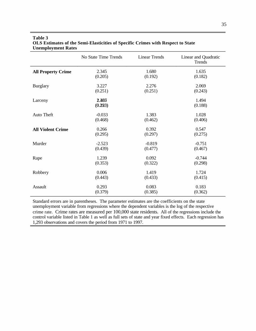
Table 3 presents separate estimates of the crime-unemployment effects for the seven specific

crimes using the same three specifications. For reference, the results for the total property and violent

crime models are reproduced. Since the results for the other control variables do not differ substantially

from the patterns presented in Table 2, we suppress this output in this and all remaining tables. Starting

with the three individual property crimes, the unemployment rate exerts positive and statistically significant

effects (at the one percent level of confidence) in all models with the exception of the auto theft regression

omitting the state-specific trends. The magnitudes of the effects are very stable across specifications again

with the exception of auto theft. For the auto theft rate, adding the trend variables drastically increases the

magnitude and significance of the unemployment rate, which points to a specific trend pattern in auto theft

18

13The relative importance of these effects in explaining recent changes in crime rates is aquestion to which we will return in the conclusion.

rates over time as compared to other crime rates. For the most complete specification, the crime-

unemployment semi-elasticities are quite similar across offenses. A one percentage point decrease in the

unemployment rate causes a two percent decrease in burglary, and 1.5 percent decrease in larceny, and

a one percent decrease in auto theft.

The results for the specific violent crimes are considerably more variable. The coefficient on

unemployment is negative for all three murder models and significant in the first two, though adding the

linear and quadratic time trends drastically reduces the magnitude of this effect. The results for rape are

unstable across specifications with a positive significant effect in the first specification, an insignificant effect

when linear trends are added, and a puzzling negative and significant effect when both linear and quadratic

time trends are included in the model. The results for robbery are stronger, with no significant effect when

time trends are omitted and significant (at one percent) positive effects in the two models that include

trends. The magnitude of the robbery-unemployment effects in the last two models are similar to the

property crime effects, a reassuring finding considering that robbery, while a violent crime in nature, is

motivated by the desire to steal someone else’s property. Finally, unemployment is insignificant in all three

assault rate models.

To summarize, we find positive and highly significant effects of unemployment on property crimes,

both in the aggregate and for individual offenses. The magnitudes of these effects are generally consistent

across specification.13 The results for violent crime are considerably weaker. For the two most serious

violent crimes of murder and rape, the effect of unemployment is either significant and wrongly-signed or

19

is unstable across specifications, while there are no measurable effects on the rate of assault and some

evidence of a positive unemployment effect for robbery.

2SLS Results

In this section, we present 2SLS estimates of the crime-unemployment semi-elasticities using

military contracts and a state-specific measure of oil costs as instruments for the state unemployment rate.

Recall, if our model specifications omit crime-determining factors that are correlated with unemployment

and that are not picked up by the fixed effects and trends variables, the OLS results that we have

presented thus far will be biased. Moreover, if crime rates reverse-cause unemployment rates, inferences

from OLS results will be flawed.

Before discussing estimates of the unemployment effects, an evaluation of the strength of the first-

stage relationship is needed. Table 4 presents the results from three first-stage regressions of

unemployment on the military spending and oil costs variables. While the table only presents the

coefficients for the two instruments, all of the control variables listed in Table 1 are included in the

specification. In all models, military spending negatively affects the unemployment rate. This effect is

significant at the one percent level in the first two specifications, but is insignificant in the final specification.

As expected, the oil costs variable exerts a strong positive effect on unemployment that is highly significant

in all three specifications. The results from F-tests of the joint significance of the two instruments are

presented in the final row. For all models, the two variables are jointly significant at the 0.0001 level of

confidence. Hence, with the exception of the military spending variable in the final specification, the first-

stage relationships are fairly strong.

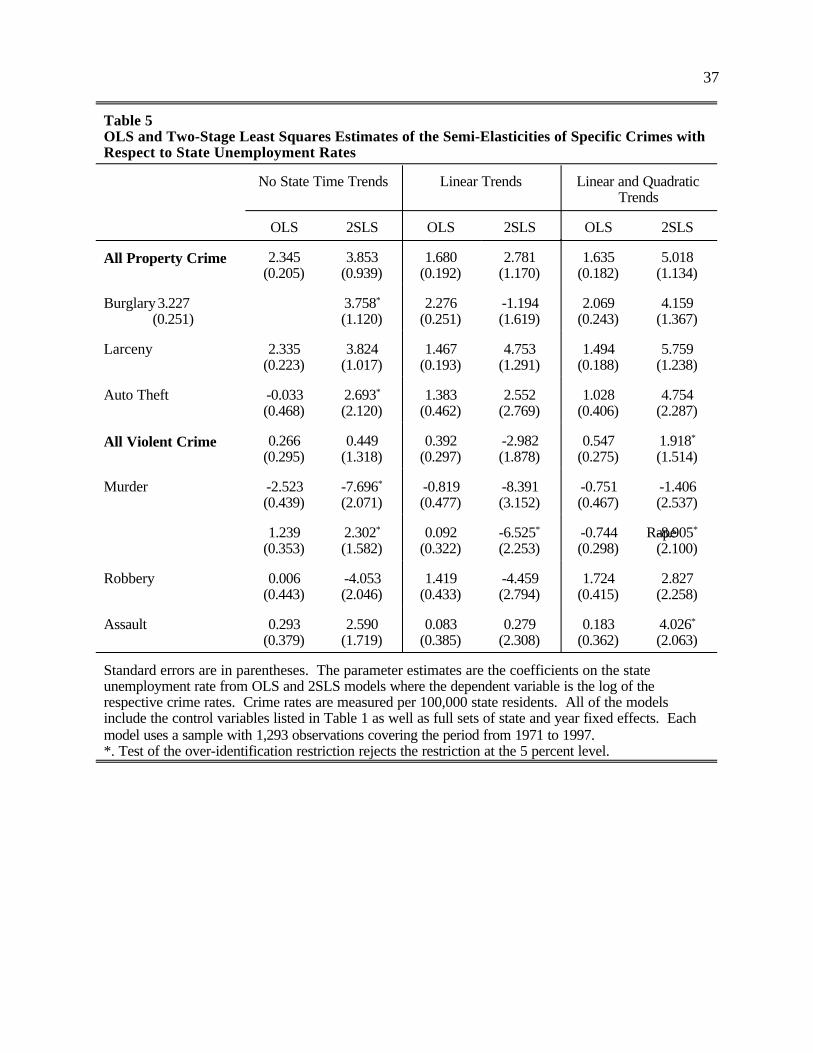
Table 5 presents the 2SLS estimates of the unemployment-crime effects for total property and

20

violent crime and for each of the seven individual crimes. Again, we only report the unemployment

coefficients and standard errors. For reference, we reproduce the OLS results from Table 3 for the three

specifications. Since we have two instruments, we can perform a test of the implicit over-identification

restriction in each model. The results of these tests are represented by the presence of an asterisk

(following the coefficient estimate) indicating tests where the restriction is rejected at the 5 percent level

of confidence. A rejection of the over-identification restriction indicates that the 2SLS estimates are

sensitive to the choice of instruments.

Similar to the OLS results, unemployment exerts consistent, positive, and highly significant effect

on the total property crime rate. For all specifications, the 2SLS results exceed the OLS results. While

the estimates from OLS range from 1.6 to 2.3, the comparable range for the 2SLS results is 2.8 to 5.0.

In contrast to the OLS findings, the strongest unemployment effect from the 2SLS models occurs in the

most complete specification. For all 2SLS specifications of the total property crime models, the over-

identification test fails to reject the restriction, thus indicating that these results are not sensitive to the choice

of instruments.

Concerning individual property crimes, the pattern is fairly similar with a few exceptions. For the

burglary rate, the 2SLS results are positive and significant at one percent in the first and third specification,

while for larceny the 2SLS results are positive and significant in all regressions. Again, when significant,

instrumenting yields stronger unemployment effects relative to OLS. For the first two auto theft models,

the unemployment effects are positive yet insignificant. In the final specification however, unemployment

exerts a large positive effect that is significant at the 5 percent level. Of the nine individual property crime

models estimated, the over-identification restriction is rejected in only two (the first specification for auto

21

14Note that these counterintuitive results are very common in the literature.

theft and burglary). Hence, we interpret the findings for property crimes in Table 5 as strongly reinforcing

the OLS results.

On the other hand, the 2SLS results for the violent crime models are not so strong. Unemployment

is insignificant in all three estimates of the total violent crime models. For murder, the 2SLS unemployment

effects are even more negative than those from the OLS regression. A similar pattern is observed for rape.

For the two specifications where we find positive OLS unemployment effects for robbery, instrumenting

yields a negative significant effect for the first (including linear time trends only) and a positive insignificant

effect for the second (including linear and quadratic time trends). The one specification where the 2SLS

model yields a positive significant unemployment effect is for the final specification of the assault rate. Here

the instrumented point estimate exceeds the OLS estimate considerably and is significant at the 5 percent

level.

5. Are the Unemployed Less Violent?

The results presented in the previous sections paint a consistent portrait of the relationship between

unemployment and property crime that confirms the simple theoretical arguments that we offer. While the

magnitude of the relationship depends to a certain degree on the estimation method used, higher

unemployment unambiguously increases property crime rates. The same, however, cannot be said for

violent crime. In fact, for the two most serious violent crimes (murder and rape) the estimated effects of

unemployment are strongly negative.14 Interpreting these results literally would indicate that an

22

15Recall, if unemployment is itself creating variation in relevant factors that we cannot observe,even our 2SLS estimates will be biased.

16Data from U.S. victimization surveys indicates that females are victims in 91.3 percent ofreported cases. For the 8.7 percent where males are victims, 0.2 percent involve a female offender and8.5 percent involve a male offender (U.S. DOJ 1997).

unemployment spell decreases one’s propensity towards violence. While possible, this seems unlikely

considering the results for property crime rates and the possibility that violence may be a byproduct of

economically motivated crimes. An alternative interpretation of these puzzling results is that in both our

OLS and 2SLS models, we have failed to account for some violence-creating factor that varies

systematically with unemployment rates.15 One candidate would be the greater frequency of interactions

between potential victims and offenders when a larger proportion of the population is working.

While in the previous section we attempted to address this issue through extensive controls and

by employing instrumental variables, here we take an alternative tack in an attempt to resolve the counter-

intuitive results for one of the violent crimes studied above. Specifically, we exploit the fact that for the

crime of rape we can separately identify the unemployment rate of the offending and victimized populations.

In the UCR, the count of reported forcible rapes is limited to incidents involving female victims. Of those

incidents,16 victimization survey results indicate that the offenders are males in over 99.5 percent of the

cases. Moreover, arrest data indicates that over 99 percent of those arrested for forcible rape are male

(U.S. DOJ 1997). Hence, for the most part, the offending population is male while the victimized

population is female.

We use this information in the following manner. Since women are not among the offenders, a

possibly negative relationship between state rape rates and female unemployment rates must be attributable

23

to factors other than a criminal behavioral response by women. Hence, if the empirical findings using

female unemployment rates parallel those using aggregate unemployment rates, the omitted-variables

interpretation is the correct one. Moreover, having identified a non-offending population, the

unemployment rate for this population can be used as an added control to estimate the behavioral

relationship between the unemployment rate of the offending population and the state rape rate.

Table 6 presents the results from this exercise. Here we use gender-specific unemployment rates

taken from the Current Population Survey Local Area Unemployment Statistics Geographic Profile Series.

Unfortunately, 1981 is the earliest year for which these data are available. To explore this relationship in

full, we present results using gender-specific employment-to-population ratios as well as unemployment

rates. The first four regressions in each panel correspond to the specification omitting trends, the next four

add linear trends, while the final four add the quadratic trends. Again, all of the variables listed in Table

1 are included in all models.

Starting with the unemployment models in Panel A, the regression in columns (1), (5), and (9)

present estimates for the aggregate unemployment rate. The pattern is similar to the results for the longer

time period in Table 3. When the trends are omitted there is a positive yet insignificant unemployment effect

(0.674), adding the linear trends yields a negative insignificant estimate (-0.305), while adding the quadratic

trends yields a negative and significant (at 5 percent) estimate of unemployment on rape (-0.937). Columns

(2), (6), and (10) present similar models where the female unemployment rate is substituted for the aggregate

rate. The pattern is quite similar, with insignificant estimates for the first two specifications and a negative

and significant point estimate in columns (10) of -0.914. Hence, the same pattern exists using the

unemployment rate for a non-offending population.

24

Columns (3), (7), and (11) use the male unemployment rate instead. Here, the first specification

yields a positive significant effect while the second and third specifications yield insignificant effects. The

point estimates for male unemployment are consistently larger than those for the female unemployment and

total unemployment rates.

Finally, in columns (4), (8), and (12), we add both the male and female unemployment rates to the

specification. In all three regressions, the coefficient on female unemployment is negative. Moreover, these

effects are significant in the first and third regressions. For male unemployment rates, all coefficient estimates

are positive with a significant effect (at the one percent level) in the first specification (column (4)). Adding

female unemployment rates increases the point estimate on the male unemployment coefficient in all models.

Hence, the results from panel A yield more sensible findings for rape than those from the previous section:

rather than being unrelated or negatively related to rape, the effects on rape of the unemployment rate of the

offending population are generally positive and sometimes significant.

Panel B presents comparable results where employment rates are substituted for unemployment

rates. Here, the “correct” sign would be negative. Using the aggregate employment rate in columns (1),

(5), and (9), we consistently find employment effects of the wrong sign. In all specifications, employment

exerts a positive and significant effect on rape. Hence, the perverse results are even stronger using

employment rates. In the models that substitute female employment rate for the aggregate rate, there is a

weakly significant positive effect in the first specification, and insignificant positive effects in the last two

specifications. In contrast, the first two specifications of the model including male employment rates only

yield weakly significant negative effects of male employment on rape rates, while in the final specification the

point estimate is effectively zero.

25

Finally, controlling for both male and female employment rates simultaneously yields results similar

to the comparable models using the unemployment rates. The coefficients on male employment become

larger (more negative) and are significant at the one and five percent level in the first and second

specification, respectively. In the final specification, the point estimate is still small and insignificant. Finally,

for the first two specifications, female employment rates exert positive significant effects while in the third

specification the variable is insignificant.

In sum, the strategy pursued in this section indicates that the “perverse“ unemployment coefficients

for some violent offenses are caused by omitted variables bias. One possible interpretation would be that

in good times exposure to offenders is higher thus masking the negative effect of unemployment on the

propensity to commit violent crimes. In the case of rape we can show that the employment prospects of

males are weakly related to rape rates. Most importantly, the results for female unemployment rates indicate

that the negative significant unemployment effects observed in Table 3 results from model mis-specification.

While this strategy cannot be applied to murder rates due to fact that there is not a similarly clear distinction

between offenders and victims, the results for rape suggest that a similar fix may yield findings in contrast to

those presented above and may therefore solve this puzzle which is very common but unresolved in the

literature.

6. Conclusion

The results presented here consistently indicate that unemployment is an important determinant of

property crime rates. The strong effects on property crimes exist in models of aggregate property crime

as well as models of the individual felonies. Moreover, the results for property crimes do not depend on

26

the estimation methodology used, although we do find relatively stronger effects when we instrument for state

unemployment rates. Hence, the results of this paper strongly confirm a basic economic model of the

determination of property crimes.

We did not find such consistency for violent crimes. In our OLS results, we find some evidence that

the economically-motivated violent crime of robbery is positively effected by unemployment rates. This

finding, however, is not reproduced when we instrument for unemployment. For the crimes of murder and

rape, our initial results indicate that unemployment is negatively related to these crimes. Upon closer

examination of the rape models, however, this paradoxical results vanishes. These findings for rape cast

doubt on a behavioral interpretation of the observed negative effects on murder – i.e., being unemployed

reduces one’s tendency to become violent and murder someone.

In the opening paragraphs, we cite the recent downward trends in crime occurring during the 1990s.

To put our results into perspective, it is instructive to work through how much of the recent declines can be

explained by the decline in unemployment rates assuming that our estimation results are valid. Since our

findings for rape indicate (1) that the unemployment effect on rape is weakly positive or insignificant, and

(2) OLS estimates of the violent crime-unemployment relationship appear to be downwardly biased by

omitted factors, we can assume that the unemployment effects on both murder and rape are zero.

Moreover, since the estimation results generally indicate that the unemployment effect on assault is zero, we

also omit this crime rate from these simple simulations. To present conservative estimates of the potential

contribution of declining unemployment, we use the OLS estimates from the most complete model

specification (Table 3, column 3).

Between 1992 and 1997 (the last six years of our panel), the rate of robbery decreased by 30

27

17See Anderson (1999) for a recent comprehensive calculation of the costs of crime to societyat large. He estimates the aggregate burden of crime - excluding the transfer of property - to more than$ 1 trillion.

percent, the rates of auto theft and burglary declined by more than 15 percent, and larceny declined by

slightly more than 4 percent. Concurrently, the unemployment rate declined from approximately 7.4 to 4.9

percent. Our OLS estimates from the most complete specification predict that the 2.5 percentage point

decline in unemployment caused a decrease of 5 percent for burglary, 3.7 percent for larceny, 2.5 percent

for auto theft, and 4.3 percent for robbery. Expressed as a percentage of actual declines, our estimates

indicate that 28 percent for the burglary rate, 82 percent for larceny, 14 percent for auto theft, and 14

percent for robbery is attributable to the decline in the unemployment rate. If we look at the overall property

crime rate, slightly more than 40 percent of the decline can be attributed to the decline in unemployment.

Note, that these are conservative estimates for two reasons: we use the OLS estimates, which are

considerably lower than the corresponding 2SLS estimates. Moreover, income per capita has in general

a negative impact on crime rates, which can be considered as an additional impact of the business cycle on

criminal behavior.

Hence, the magnitudes of the crime-unemployment effects presented here relative to overall

movements in crime rates are substantial and suggest that policies aimed at improving the employment

prospects of workers facing the greatest obstacles can be effective tools for combating crime.17 Moreover,

given that crime rates in the U.S. are considerably higher in areas with high concentrations of jobless

workers (many inner-city communities, for example) and the fact that those workers with arguably the worst

employment prospects (young African-American males) are the most likely to be involved with the criminal

28

justice system, employment-based anti-crime policies contains the attractive feature of being consistent with

a wide-range of policy objectives.

29

References

Anderson, David A. (1999), “The Aggregate Burden of Crime“, Journal of Law and Economics 42, 611-642.

Blanchard, Olivier Jean and Lawrence F. Katz (1992), "Regional Evolutions", Brookings Papers onEconomic Activity, 1: 1-75.

Bound John and Richard B. Freeman (1992), "What Went Wrong? The Erosion of Relative Earnings andEmployment Among Young Black Men in the 1980s", Quarterly Journal of Economics 107, 201-231.

Boyum, David and Mark A. R. Kleiman (1995), "Alcohol and Other Drugs," in James Q. Wilson and JoanPetersilia (eds.) Crime, ICS Press, San Francisco, pp. 295-326.

Bushway, Shawn and John Engberg (1994), "Panel Data VAR Analysis of the Relationship betweenCrime and Unemployment", mimeo, Carnegie Mellon University.

Chiricos, Theodor (1987), "Rates of Crime and Unemployment: An Analysis of Aggregate ResearchEvidence," Social Problems 34(2): 187-211.

Cook, Philip J. and Mark H. Moore (1995), "Gun Control," in James Q. Wilson and Joan Petersilia (eds.)Crime, ICS Press, San Francisco, pp. 295-326.

Cook, Philip J. and Gary A. Zarkin (1985), "Crime and the Business Cycle," Journal of Legal Studies14(1): 115-128.

Corman, Hope, Joyce, Theodor and Norman Lovitch (1987), "Crime, Deterrence and the Business Cyclein New York City: A VAR Approach", Review of Economics and Statistics 69, 695-700.

Corman, Hope and H. Naci Mocan (2000), “A Time-Series Analysis of Crime, Deterrence and DrugAbuse in New York City“, American Economic Review, forthcoming.

Davis, Steven J., Loungani, Prakash and Ramamohan Malidhara (1997), "Regional Labor Fluctuations:Oil Shocks, Military Spending, and other Driving Forces" , Board of Governors of the Federal ReserveSystem, IF Working Paper # 578.

Entorf, Horst and Hannes Spengler (2000), "Socio-economic and Demographic Factors of Crime inGermany: Evidence from Panel Data of the German States", International Review of Law andEconomics, forthcoming.

Fagan, Jeffrey (1990), “Intoxication and Aggression,” in Michael H. Tonry and James Q. Wilson (eds.)Drugs and Crime, pp. 241-320, volume 13 of Crime and Justice: A Review of Research, Chicago:

30

University of Chicago Press.

Freeman, Scott, Jeff Grogger and Jon Sonstelie (1996), "The Spatial Concentration of Crime", Journal ofUrban Economics 40, 216-231.

Friedberg, Leora (1998), “Did Unilateral Divorce Raise Divorce Rates? Evidence from Panel Data,”American Economic Review, 88(3): 608-627.

Gould, Eric D.; Weinberg, Bruce A.; and David B. Mustard (1998), “Crime Rates and Local Labor MarketOpportunities in the United States: 1979-1995,” unpublished manuscript.

Greenberg, David F. (1985), “Age, Crime, and Social Explanation,” American Journal of Sociology,91(1): 1-21.

Greenberg, Edward (1967), "Employment Impacts of Defense Expenditures and Obligations," Review ofEconomics and Statistics, 49(2): 186-198.

Grogger, Jeff (1995), "The Effect of Arrest on the Employment and Earnings of Young Men", QuarterlyJournal of Economics 110, 51-72.

Grogger, Jeff (1998), “Market Wages and Youth Crime,” Journal of Labor Economics, 16(4): 756-791.

Hirshi, Travis and Michael Gottfredson (1983), “Age and the Explanation of Crime,” American Journalof Sociology, 89(3): 552-584.

Hooker, Mark A. and Michael M. Knetter (1994), “Unemployment Effects of Military Spending: Evidencefrom a Panel of States,” National Bureau of Economic Research Working Paper #4889.

Hooker, Mark A. and Michael M. Knetter (1997), "The Effects of Military Spending on Economic Activity:Evidence from State Procurement Spending," Journal of Money, Credit and Banking, 28(3).

Levitt, Steven D. (1996), "The Effect of Prison Population Size on Crime Rates: Evidence from PrisonOvercrowding Litigation," Quarterly Journal of Economics 111, 319-353.

Levitt, Steven D. (1997), “Using Electoral Cycles in Police Hiring to Estimate the Effect of Police onCrime,” American Economic Review, 87(3): 270-290.

Machin, Stephen and Costas Meghir (2000), “Crime and Economic Incentives,“ mimeo, UniversityCollege, London.

Marvell, Thomas B. and Carlisle E. Moody (1995), "The Impact of Enhanced Prison Terms for Felonies

31

Committed With Guns," Criminology, 33: 247-249.

Marvell, Thomas B. and Carlisle E. Moody (1996), "Determinate Sentencing and Abolishing Parole: TheLong-Term Impacts on Prisons and Crime," Criminology, 34(1): 107-128.

Mayer, Kenneth R. (1991), The Political Economy of Defense Spending, Yale University Press: NewHaven and London.

Nagin, Daniel and Joel Waldfogel (1995), "The Effects of Criminality and Conviction on the Labor MarketStatus of Young British Offenders", International Review of Law and Economics 15, 109-126.

Papps, Kerry and Rainer Winkelman (1998), "Unemployment and Crime: New Answers to an OldQuestion," unpublished manuscript, University of Canterbury, New Zealand.

Rennison, Callie M. (1999), “Criminal Victimization 1998: Changes 1997-1998 with Trends 1993-1998,”U.S. Department of Justice Report # NCJ 1766353.

Ruhm, Christopher J. (1995), "Economic Conditions and Alcohol Problems," Journal of HealthEconomics 14, 583-603.

U. S. Department of Justice (1997), “Sex Offenses and Offenders: An Analysis of Data on Rape andSexual Assault,” Bureau of Justice Statistics Report #NCJ-163392.

Willis, Michael (1999a), "Crime and the Location of Jobs" , Working Paper, University of California,Santa Barbara.

Willis, Michael (1999b), “Unemployment, the Minimum Wage, and Crime“, University of California, SantaBarbara.

Witte, Ann Dryden and Helen Tauchen (1994), Work and Crime: An Exploration Using Panel Data,NBER Working Paper # 4794.

32

A

B

C

D

E U0

U1

Non-Market Time

Income

t0t1 A

B

C

D

t0Non-Market Time

IncomeFigure 1A Figure 1B

Figure 1

33

Table 1Summary Statistics

Variables Means Standard Deviation Standard DeviationNet of State and Time

effects

Property Crime Burglary Larceny Auto Theft

4,674.811,276.262,883.48

515.07

1,158.20419.12725.10229.48

434.24162.58268.6792.77

Violent Crime Murder Rape Robbery Assault

585.518.58

34.36220.07322.51

264.353.49

11.67132.17156.99

68.851.295.97

29.8151.96

UnemployedPrison PopulationAlcohol ConsumptionMetropolitanPoorBlackIncome per worker

Population <15Population 15-17Population 18-24Population 25-34Population 35-44Population 45-54Population 55-64

0.07214.03

1.980.770.130.11

33.39

0.230.050.120.160.130.110.09

0.02134.13

0.400.170.040.07

14.13

0.030.010.020.020.020.010.01

0.01 45.360.150.020.020.012.32

0.0070.0020.0050.0070.0040.0030.003

Military SpendingOil Costs

0.380.16

0.310.09

0.140.03

All crime rate as well as the incarceration rate in state prisons are defined per 100,000 state residents. Alcohol consumption is measured in consumption of gallons of ethanol per capita. Income per workerand military spending are measured in thousands of dollars per capita. The panel covers the periodfrom 1971 to 1997. There are 1,293 observations.

34

Table 2OLS Regressions of Total Property and Total Violent Crime on State Unemployment Ratesand Variables Measuring State Demographic Structure

ln(Property Crime Rate) ln(Violent Crime Rate)

(1) (2) (3) (4) (5) (6)

Unemployed 2.345(0.205)

1.680(0.192)

1.635(0.182)

0.266(0.295)

0.392(0.297)

0.547(0.275)

ln(Prisoners) -0.129(0.015)

-0.093(0.014)

-0.108(0.015)

-0.018(0.021)

-0.028(0.022)

-0.042(0.022)

AlcoholConsumption

0.207(0.023)

-0.147(0.028)

-0.129(0.028)

0.074(0.034)

0.048(0.044)

0.027(0.043)

Metropolitan 0.875(0.148)

0.670(0.185)0.145

(0.232)0.754

(0.212)1.510

(0.286)0.922

(0.350)

Poor -1.081(0.156)

-0.207(0.131)

0.076(0.128)

-0.209(0.223)

-0.195(0.202)

-0.247(0.194)

Black 1.508(0.414)

-2.883(0.807)

3.881(1.475)

-3.475(0.594)

-2.987(1.246)

5.024(2.229)

Income PerWorker

-0.010(.001)

-0.025(0.002)

-0.001(0.004)

-0.012(0.002)

-0.022(0.004)

-0.016(0.005)

Population < 15 -1.841(0.469)

0.817(0.479)

0.014(0.637)

0.016(0.674)

-1.412(0.739)

-4.006(0.963)

Population15 to 17

8.338(1.734)

14.379(1.700)

10.360(1.770)

7.064(2.487)

4.729(2.625)

9.758(2.676)

Population 18 to 24

0.637(0.676)

1.367(0.578)

1.466(0.633)

2.326(0.971)

1.789(0.893)

4.551(0.956)

Population 25 to 34

1.395(0.588)

7.123(0.564)

7.611(0.718)

7.277(0.844)

7.127(0.871)

7.474(1.086)

Population 35 to 44

-5.862(0.756)

-1.666(0.890)

-0.525(1.178)

1.174(1.086)

0.569(1.374)

-6.398(1.781)

Population45 to 54

2.206(0.917)

5.508(1.096)

4.825(1.498)-2.797(1.315)

-2.805(1.693)

-1.305(2.264)

Population 55 to 64

-4.751(0.974)

-5.189(0.921)

-3.575(1.495)

-0.238(1.397)

0.376(1.421)

7.120(2.261)

Linear Trends No Yes Yes No Yes Yes

Quadratic Trends No No Yes No No Yes

Standard errors are in parentheses. The dependent variable in each regression is the log of therespective crime rate per 100,000 state residents. All regression include a full set of state and year fixedeffects. There are 1,293 observations covering the periods from 1971 to 1997.

35

Table 3OLS Estimates of the Semi-Elasticities of Specific Crimes with Respect to StateUnemployment Rates

No State Time Trends Linear Trends Linear and QuadraticTrends

All Property Crime 2.345(0.205)

1.680(0.192)

1.635(0.182)

Burglary 3.227(0.251)

2.276(0.251)

2.069(0.243)

Larceny 2.335(0.223)1.467

(0.193)1.494

(0.188)

Auto Theft -0.033(0.468)

1.383(0.462)

1.028(0.406)

All Violent Crime 0.266(0.295)

0.392(0.297)

0.547(0.275)

Murder -2.523(0.439)

-0.819(0.477)

-0.751(0.467)

Rape 1.239(0.353)

0.092(0.322)

-0.744(0.298)

Robbery 0.006(0.443)

1.419(0.433)

1.724(0.415)

Assault 0.293(0.379)

0.083(0.385)

0.183(0.362)

Standard errors are in parentheses. The parameter estimates are the coefficients on the stateunemployment variable from regressions where the dependent variables is the log of the respectivecrime rate. Crime rates are measured per 100,000 state residents. All of the regressions include thecontrol variable listed in Table 1 as well as full sets of state and year fixed effects. Each regression has1,293 observations and covers the period from 1971 to 1997.

36

Table 4First-Stage Regressions of State Unemployment Rates on State Military Contracts PreCapita and State Level Measure of Oil Costs

(1) (2) (3)

Military Spending -0.012(0.002)-0.007(0.002)

-0.004(0.003)

Oil Costs 0.091(0.014)

0.064(0.013)

0.088(0.015)

Linear Trends No Yes Yes

Quadratic Trends No No Yes

F-Statistica

(P-Value)31.783

(0.0001)16.571

(0.0001)19.377(.0001)

Standard errors are in parentheses. All of the regressions include the control variables listed in Table1 as well as full sets of state and year fixed effects. Each regression has 1,293 observations andcovers the period from 1971 to 1997.a. This is the test statistic (and p-value) from an F-test of the joint significance of the military spendingand oil costs instrumental variables.

37

Table 5OLS and Two-Stage Least Squares Estimates of the Semi-Elasticities of Specific Crimes withRespect to State Unemployment Rates

No State Time Trends Linear Trends Linear and QuadraticTrends

OLS 2SLS OLS 2SLS OLS 2SLS

All Property Crime 2.345(0.205)

3.853(0.939)

1.680(0.192)

2.781(1.170)

1.635(0.182)

5.018(1.134)

Burglary3.227(0.251)

3.758*

(1.120)2.276

(0.251)-1.194(1.619)

2.069(0.243)

4.159(1.367)

Larceny 2.335(0.223)

3.824(1.017)

1.467(0.193)

4.753(1.291)

1.494(0.188)

5.759(1.238)

Auto Theft -0.033(0.468)

2.693*

(2.120)1.383

(0.462)2.552

(2.769)1.028

(0.406)4.754

(2.287)

All Violent Crime 0.266(0.295)

0.449(1.318)

0.392(0.297)

-2.982(1.878)

0.547(0.275)

1.918*

(1.514)

Murder -2.523(0.439)

-7.696*

(2.071)-0.819(0.477)

-8.391(3.152)

-0.751(0.467)

-1.406(2.537)

Rape1.239(0.353)

2.302*

(1.582)0.092

(0.322)-6.525*

(2.253)-0.744(0.298)

-8.905*

(2.100)

Robbery 0.006(0.443)

-4.053(2.046)

1.419(0.433)

-4.459(2.794)

1.724(0.415)

2.827(2.258)

Assault 0.293(0.379)

2.590(1.719)

0.083(0.385)

0.279(2.308)

0.183(0.362)

4.026*

(2.063)

Standard errors are in parentheses. The parameter estimates are the coefficients on the stateunemployment rate from OLS and 2SLS models where the dependent variable is the log of therespective crime rates. Crime rates are measured per 100,000 state residents. All of the modelsinclude the control variables listed in Table 1 as well as full sets of state and year fixed effects. Eachmodel uses a sample with 1,293 observations covering the period from 1971 to 1997.*. Test of the over-identification restriction rejects the restriction at the 5 percent level.