I d e n t i f y i n g u n e x p e c t e d a c c r u a l s :

a c o m p a r i s o n o f c u r r e n t a p p r o a c h e s

Jacob Thomas 620 Uris Hall

Columbia Business School New York, NY 10027

E-mail: jkt1@columbia.edu Phone: (212) 854-3492

and

Xiao-jun Zhang†

June 2000 † Jacob Thomas is Ernst & Young Professor of Accounting and Finance at the Columbia

Business School, and Xiao-jun Zhang is Assistant Professor of Accounting at the University of California-Berkeley. We received helpful comments from Dan Beneish, Paul Healy, and Steve Loeb and workshop participants at CUNY-Baruch College, University of Florida, and M.I.T.

I d e n t i f y i n g u n e x p e c t e d a c c r u a l s :

a c o m p a r i s o n o f c u r r e n t a p p r o a c h e s

Abstract

While prior research, as noted in our paper, often uses various accrual prediction models to detect earnings management, not much is known about the accuracy, both relative and absolute, associated with these models. Our paper investigates the accuracy of six different accrual prediction models, and offers the following findings. Only the Kang-Sivaramakrishnan (1995) model performs moderately well. The remaining five models provide little ability to predict total accruals: they are less accurate than a naïve model which predicts that total accruals equal -5 percent of total assets for all firms and years. Conventional R2 values from a regression of actual accruals on predicted accruals are less than zero for a substantial majority of firms for these five models. These low R2 values in the prediction period contrast sharply with the much higher R2 values that are obtained within the estimation period. Similar performance is observed when predicting current accruals alone. However, the relative rankings of the different models are altered somewhat: the Jones (1991) model is then the only model that exhibits some predictive ability.

I d e n t i f y i n g u n e x p e c t e d a c c r u a l s : a c o m p a r i s o n o f c u r r e n t a p p r o a c h e s

1. Introduction

Numerous studies have used a variety of accrual prediction models for different

objectives. Typically, these models have been used to detect earnings management. Earnings

are hypothesized to have been managed in predictable ways in response to certain incentives

(e.g. Watts and Zimmerman, 1986, and Schipper, 1989), and the discretionary accruals used to

manage earnings are estimated from these accrual prediction models. Examples include studies

of earnings management due to compensation agreements (Healy, 1985; Gaver et al., 1995; and

Holthausen et al., 1995), proxy contests (DeAngelo, 1988), and lobbying for trade restrictions

(Jones, 1991).1 Usually, realized accruals are compared with forecasts from an accrual

prediction model, and the forecast errors are assumed to represent discretionary accruals, or

earnings management. In effect, forecast accruals are assumed to represent non-discretionary

accruals, the accruals that would be observed absent any incentives to manage earnings.

While these models have been used often, little attention has been paid to the relative or

absolute accuracy of different accrual models. Two recent studies that have examined the

accuracy of accrual models are Dechow et al. (1995) and Kang and Sivaramakrishnan (1995).

Both papers examine the ability of different models to identify type I errors (reject the null

hypothesis of no earnings management when it is true) and type II errors (fail to reject the null

hypothesis when it is false). They have also offered insights about extant models and innovative

ways to improve the ability to detect earnings management.

Our paper continues in the same vein, but is focused on the more general issue of

forecasting accruals, rather than detecting earnings management per se. Of course, the two

1 Other contexts in which earnings management has been studied include valuation, corporate control, and

financial distress. Examples of such studies include Bartov (1993), DeAngelo (1986), DeAngelo et al. (1994), DeFond and Jiambalvo (1994), Guay et al. (1996), Guenther (1994), Kang and Sivaramakrishnan (1995), Pourciau (1993), Perry and Williams (1994), and Subramanyam (1996). While most studies examine accruals, some have focused on the choice of accounting methods to infer earnings management. Studies in this group include Dhaliwal et al. (1982), and Skinner (1993).

2

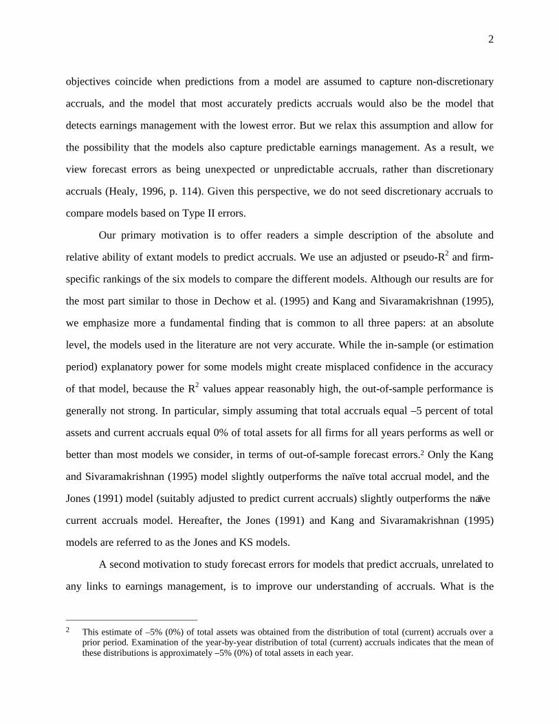
objectives coincide when predictions from a model are assumed to capture non-discretionary

accruals, and the model that most accurately predicts accruals would also be the model that

detects earnings management with the lowest error. But we relax this assumption and allow for

the possibility that the models also capture predictable earnings management. As a result, we

view forecast errors as being unexpected or unpredictable accruals, rather than discretionary

accruals (Healy, 1996, p. 114). Given this perspective, we do not seed discretionary accruals to

compare models based on Type II errors.

Our primary motivation is to offer readers a simple description of the absolute and

relative ability of extant models to predict accruals. We use an adjusted or pseudo-R2 and firm-

specific rankings of the six models to compare the different models. Although our results are for

the most part similar to those in Dechow et al. (1995) and Kang and Sivaramakrishnan (1995),

we emphasize more a fundamental finding that is common to all three papers: at an absolute

level, the models used in the literature are not very accurate. While the in-sample (or estimation

period) explanatory power for some models might create misplaced confidence in the accuracy

of that model, because the R2 values appear reasonably high, the out-of-sample performance is

generally not strong. In particular, simply assuming that total accruals equal –5 percent of total

assets and current accruals equal 0% of total assets for all firms for all years performs as well or

better than most models we consider, in terms of out-of-sample forecast errors.2 Only the Kang

and Sivaramakrishnan (1995) model slightly outperforms the naïve total accrual model, and the

Jones (1991) model (suitably adjusted to predict current accruals) slightly outperforms the naïve

current accruals model. Hereafter, the Jones (1991) and Kang and Sivaramakrishnan (1995)

models are referred to as the Jones and KS models.

A second motivation to study forecast errors for models that predict accruals, unrelated to

any links to earnings management, is to improve our understanding of accruals. What is the

2 This estimate of –5% (0%) of total assets was obtained from the distribution of total (current) accruals over a

prior period. Examination of the year-by-year distribution of total (current) accruals indicates that the mean of these distributions is approximately –5% (0%) of total assets in each year.

3

cross-sectional and time-series correlation structure among forecast errors? How much of the

variation in total accruals is due to each of its components: current and noncurrent accruals?

What is the correlation of forecast errors across models, and how much is gained by combining

forecasts from different accrual prediction models? Examination of forecast errors from a

variety of accrual prediction models allows us to provide answers to these questions. Given that

accruals lie at the core of accounting, additional understanding of the behavior of accruals should

be valuable to all aspects of accounting thought.

A more detailed discussion of the similarities and differences between discretionary

accruals and unexpected accruals is laid out in section 2. Section 3 offers a description of the

different accrual models considered. In Section 4, we report the primary results based on accrual

forecasts for a sample of 1,748 Compustat firms over the 5-year period between 1990 and 1994.

In addition to reporting the distribution of forecast errors and a pseudo-R2 for the forecast period,

we also provide a simple nonparametric analysis: each model is ranked (first through sixth) in

terms of mean squared error for each firm and the distribution of ranks reported across the

sample. Section 5 contains the results of extensions to the primary analysis, and Section 6

concludes.

2. Unexpected accruals versus discretionary accruals.

Despite our focus on the properties of forecast accruals per se, we consider briefly in this

section the relation between forecast errors from accrual prediction models (unexpected accruals)

and the ability to detect earnings management (discretionary accruals).

Consider the usual separation of total accruals (TOTACCit), for firm i in year t, into the

following two parts: true discretionary (DISCACCit) and true non-discretionary accruals

(NONDISCACCit).

TOTACCit = NONDISCACCit + DISCACCit …(1)

4

Each model then generates a forecast for total accruals (^

itTOTACC ), which can in turn

be viewed as the sum of the forecasted values of non-discretionary (^

itNONDISCACC ) and

discretionary accruals (^

itDISCACC ). Therefore, forecast errors (FEit) from each model can be

viewed as the sum of forecast errors on the two components of total accruals.

^

itit

^

itit

^

ititit DISCACCDISCACCNONDISCACC NONDISCACCTOTACC TOTACCFE −+−=−= …(2)

Since the researcher in general observes only total accruals,3 it is hard to draw links

between FEit and DISCACCit, without imposing additional structure. The prior literature has

assumed that discretionary accruals are negligible during the estimation period, and the model

used is in effect derived for non-discretionary accruals alone (e.g., Dechow et al., 1995, p. 195).

As a result, any forecast error in the period of suspected earnings management is viewed as a

reasonable estimate for discretionary accruals in that period. If, however, discretionary accruals

exist even in the estimation period, the models revert to predicting unexpected accruals, since the

predictable portion of both non-discretionary and discretionary accruals is captured in the

forecast.4

There are two important differences between a methodological study such as ours and the

typical earnings management study. First, unlike studies that examine accruals around events

hypothesized to have caused firms to manage earnings, there is no reason to expect more

earnings management in our non-event forecast period. That is, the estimation and forecast

periods are conceptually similar in our study, and are drawn from the same underlying

population. Second, when evaluating the relative performance of different models, we are

comparing the distribution of forecast errors across models for the same forecast firm-years. In

3 It has been suggested that discretionary accruals are easier to detect if researchers focus on any one component

of accruals, rather than on total accruals (see Beneish, 1998a, pp. 86-87). McNichols and Wilson (1988) and Miller and Skinner (1998) are examples of such studies.

4 If, for example, revenue changes predicted both non-discretionary accruals as well as some portion of discretionary accruals, then an accrual model which uses revenue changes as an explanatory variable would capture that portion of discretionary accruals in its forecast of non-discretionary accruals.

5

effect, each firm-year serves as its own control, and the level of true discretionary and non-

discretionary accruals are held constant across the different models for each firm-year.

The links between forecast errors and discretionary accruals that can be forged from our

study are a function of the structure imposed on discretionary and non-discretionary accruals in

non-event (estimation) periods. If, discretionary accruals are rare, then forecast errors can be

used to offers insights about the absolute and relative ability of each model to predict non-

discretionary accruals in non-event periods. These forecast errors also represent the error with

which discretionary accruals will be measured in an event period with systematic earnings

management when that particular model is used.5

On the other hand, if non-event periods are associated with substantial earnings

management, forecast errors cannot be used to make statements about the absolute level of

earnings management in event-periods. Some inferences about the relative ability (across

models) to detect earnings management in event periods are possible, however, given certain

assumptions about the relation between forecast errors for discretionary and non-discretionary

accruals.6

In sum, if forecast errors provide information about the absolute level of discretionary

accruals, our study adds to the literature on errors in detecting earnings management. If,

however, forecast errors are informative only about the relative ability of different models to

detect earnings management, our study helps to rank the performance of these models. Even if

no inferences are possible about the absolute or relative ability of the six models to identify

earnings management, we believe that accruals are important enough on their own to merit some

study of their properties.

5 Since the forecast error associated with non-discretionary accruals in a non-event period remains for event

periods, the error associated with the discretionary accruals in an event period would then be of the same magnitude but of opposite sign.

6 If, for example, the two errors are independent during non-event periods, the variance of forecast errors should be inversely related to the relative ability of each model to identify discretionary accruals.

6

3. The accrual prediction models

Before discussing the different accrual prediction models, it is useful to define accruals

and describe the measures used in the empirical literature. Total accruals are usually defined

(e.g., Dechow et al., 1995, p. 203) as the difference between net income (NIit) and cash flow

from operations (CFOit).

TOTACCit = NIit - CFOit …(3)

Rather than compute total accruals from net income and cash flow from operations, it is

usually represented by approximate measures for the following two components: current accruals

(CURACCit), proxied by the change in working capital (excluding cash), and noncurrent accrual

(NONCURACCit), proxied by depreciation, depletion, and amortization (e.g., Dechow et al.,

1995, p. 203). In effect, all other accrual items are ignored.

TOTACCit = CURACCit + NONCURACCit = ∆[(#4−#1) − #5] − #125 …(4)

where ∆ represents the year-to-year change, and the various #n represent data items from

Compustat (#4=current assets, #1=cash, #5=current liabilities, and #125=depreciation, depletion,

and amortization from the cash flow statement). The KS model is slightly different, and predicts

the balance sheet levels of accounts represented in current accruals, rather than changes in those

accounts, and includes amortization from the income statement (#14), rather than amortization

from the cash flow statement (Kang and Sivaramakrishnan, 1995, p. 358). To allow comparisons

across firms, accrual measures in all models are typically scaled by total assets from the previous

year (TAit-1), obtained from data item #6 of Compustat.

The different accrual prediction models fall into two broad categories: those that do and

those that do not peek ahead. A peek-ahead model (e.g., Jones, 1991, p. 211) uses information

from the year being forecasted, whereas the models that do not peek ahead (e.g., DeAngelo,

1986, p. 409) are limited to information available as of the prior year. Since peek-ahead models

access more current information, they might reasonably be expected to perform better than

7

models that do not peek ahead. Depending on the context of the investigation, peek-ahead

models may or may not be appropriate. For example, peek-ahead models are appropriate for

detecting earnings management, but not for examining investment strategies based on prediction

of future unexpected accruals (e.g., Sloan, 1996). For our primary analysis we consider a total of

six models: three non-peek-ahead models and three peek-ahead models.

In extensions to the primary analysis, we consider modifications to these models, and

also consider predictions of current accruals alone, rather than total accruals. This last extension

is motivated by the presumption that even though the magnitudes of noncurrent accruals exceed

those of current accruals, there is more management of current accruals than there is of

noncurrent accruals.7 Brief descriptions of the six models are provided next, and details of the

variables used are provided in the Appendix.

3.1 Random walk Model

After noting various limitations of the random walk model as a predictor of accruals,

DeAngelo (1986, p. 409) proposes it as a convenient first approximation of how

nondiscretionary accruals behave. To allow comparisons across firms, her model has typically

been adapted slightly in prior research (e.g., Dechow et al., 1995, p. 198) and applied to scaled

accruals, rather than the unscaled accruals she used.8 This adapted version of the DeAngelo

model can be represented as follows.

TOTACCit

TAit-1 =

TOTACCit-1TAit-2

+ eit …(5)

The random walk model is relatively simple to use: no estimation period is required, unlike other

models, and first differences in scaled accruals represent forecast errors.

7 Beneish (1998b, p. 211) argues that managing earnings via depreciation is potentially transparent (because

changes in estimates that alter depreciation expense are disclosed in footnotes) and economically implausible (because the timing of capital expenditures would need to be divorced partially from the arrival of profitable investment opportunities).

8 DeAngelo (1986, p. 414) also considered scaled accruals for her study, but the results remained fairly similar.

8

3.2 Mean-reverting accruals.

Accruals, especially the current accrual component, have been shown to vary from a

random walk and exhibit mean reversion (e.g., Dechow 1994, p. 18). Based on this insight,

Dechow et al. (1995, p. 197) used the mean of the past five years’ accruals as an expectation for

this year’s accrual.9

TOTACCit

TAit-1 =

15

∑τ=t-5

t-1

TOTACCiτ

TAiτ-1 + eit …(6)

Unlike the random walk model, which is influenced entirely by last year's accrual, the mean-

reverting model gives equal weight to accruals from each of the prior five years. As a result,

however, accruals cannot be forecast if missing values of scaled accruals exist for any of the

previous five years.

3.3 Components model

The random walk and mean-reverting models described above can be viewed as

representing polar opposite processes for total accruals. We speculate that a process that falls in

between these two extremes might better represent accruals. That is, total accruals might be

better represented by a weighted average of the random walk and mean-reverting models. Also,

given that current accruals exhibit more mean reversion than noncurrent accruals, predictions

should improve if current and noncurrent accruals are allowed to have separate weights. The

specific models we estimate are as follows.

9 Recently, a few papers have labeled this model the Healy model (e.g., Dechow et al., 1995, p. 197; Guay et al.,

1996, p. 83). Although Healy (1985, p. 86) expects non-discretionary accruals to equal zero, his tests effectively assume that non-discretionary accruals for each firm equal the mean accrual of all other firm-years in his sample (since his tests are based on comparisons of mean accruals across portfolios of firm-years with different predictions for discretionary accruals). Thus, the mean-reverting model above is slightly different from that used in Healy (1985), because it is based on a time-series firm-specific mean, rather than a cross-sectional mean.

9

CURACCit

TAit-1 = (α)

CURACCit-1TAit-2

+ (1-α)

15 ∑

τ=t-5

t-1

CURACCiτ

TAiτ-1 + eit …(7)

NONCURACCit

TAit-1 = (β)

NONCURACCit-1TAit-2

+ (1-β)

15 ∑

τ=t-5

t-1

NONCURACCiτ

TAiτ-1 + eit …(8)

The weights, α and β, are estimated over all firm-years with available data in the estimation

period 1975-1989, and the requirements for non-missing prior period accruals are similar to

those for the mean-reverting model. For firm years in the prediction period, the weights from the

estimation period are used to obtain predictions for current and noncurrent accruals, which are

then summed to yield a predicted total accrual.10

3.4 Jones model

The Jones model uses changes in revenues (Compustat data item #12) from period t-1 to t

and period t gross plant, property, and equipment (Compustat item # 7) to predict total accruals,

as follows (Jones, 1991, p. 211).

TOTACCit

TAit-1 = ai

1TAit-1

+ b1i ∆REVitTAit-1

+ b2i PPEitTAit-1

+ eit …(9)

Equation (9) is fitted over an estimation period for each firm i, to provide the three parameter

estimates (ai, b1i, and b2i). These estimates are then used to forecast non-discretionary accruals

in prediction periods, using values of the explanatory variables from those periods. That is, the

Jones model is a peek-ahead model, unlike the first three models. Also, since the relation is

estimated separately for each firm, only firms with sufficient years of non-missing data in the

estimation period (10 years) are included in the sample.

10 Note that the weights do not have firm subscripts, which requires that all firms have the same weights for

current and noncurrent accruals. We also examined predictions based on firm-specific weights, but found substantially greater prediction errors. Apparently, the errors in estimating weights from a limited number of time-series observations exceed the errors caused by forcing all firms to fit the same profile.

10

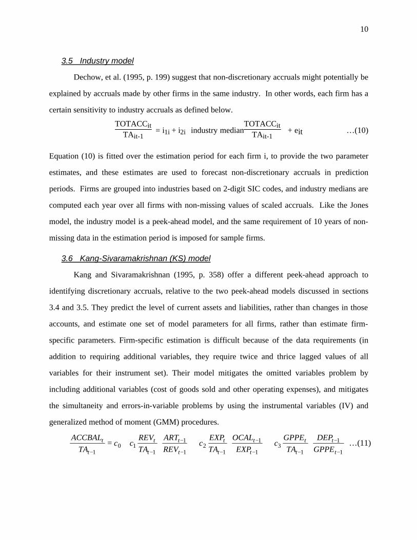
3.5 Industry model

Dechow, et al. (1995, p. 199) suggest that non-discretionary accruals might potentially be

explained by accruals made by other firms in the same industry. In other words, each firm has a

certain sensitivity to industry accruals as defined below.

TOTACCit

TAit-1 = i1i + i2i

industry medianTOTACCit

TAit-1 + eit …(10)

Equation (10) is fitted over the estimation period for each firm i, to provide the two parameter

estimates, and these estimates are used to forecast non-discretionary accruals in prediction

periods. Firms are grouped into industries based on 2-digit SIC codes, and industry medians are

computed each year over all firms with non-missing values of scaled accruals. Like the Jones

model, the industry model is a peek-ahead model, and the same requirement of 10 years of non-

missing data in the estimation period is imposed for sample firms.

3.6 Kang-Sivaramakrishnan (KS) model

Kang and Sivaramakrishnan (1995, p. 358) offer a different peek-ahead approach to

identifying discretionary accruals, relative to the two peek-ahead models discussed in sections

3.4 and 3.5. They predict the level of current assets and liabilities, rather than changes in those

accounts, and estimate one set of model parameters for all firms, rather than estimate firm-

specific parameters. Firm-specific estimation is difficult because of the data requirements (in

addition to requiring additional variables, they require twice and thrice lagged values of all

variables for their instrument set). Their model mitigates the omitted variables problem by

including additional variables (cost of goods sold and other operating expenses), and mitigates

the simultaneity and errors-in-variable problems by using the instrumental variables (IV) and

generalized method of moment (GMM) procedures.

+

+

+=

−

−

−−

−

−−

−

−− 1

1

13

1

1

12

1

1

110

1 t

t

t

t

t

t

t

t

t

t

t

t

t

t

GPPE

DEP

TA

GPPEc

EXP

OCAL

TA

EXPc

REV

ART

TA

REVcc

TA

ACCBAL…(11)

11

Our Appendix provides details of the variables in equation (11). Based on results in Kang

(1999, p. 4), which indicate that the IV and GMM procedures provide very similar results, we

consider only the IV procedure.

3.7 Other models

We report on results obtained from some of the other models that have been proposed in

the literature. Boynton et al. (1992, p. 137) estimate the Jones model using data pooled for each

industry, rather than estimate the model separately for each firm. Boynton et al. (1992) only

include the five most recent years in the estimation period to minimize problems caused by

potential non-stationarity. We consider this modification in section 5 and confirm that the results

are indeed better than the traditional Jones model, in terms of forecast accuracy. Beneish (1997,

p. 273) suggests that lagged total accruals and contemporaneous price performance be also

included to improve the Jones model. We examine these modifications too but are unable to find

much improvement over the Jones model (see discussion in section 5).

Dechow et al (1995, p. 199) propose a modification of the Jones model which removes

changes in net account receivables from the revenue changes used as an explanatory variable in

equation (9). Note that this adjustment is only made in the test period, and the standard Jones

model is fitted in the estimation period. Dechow et al. (1995, p. 199) argue that earnings

management might influence reported revenue numbers and such an adjustment mitigates the

effect of earnings management on this explanatory variable. We do not examine this

modification of the Jones model, as it applies only to firms that are ex ante likely to undertake

earnings management. Examining all firms in the population, many of which are unlikely to

have managed earnings, creates the potential of increasing forecast errors by changing the model

for such firms between the estimation and forecast periods.

4. Sample selection and results

Financial data were obtained from the 1995 editions of the annual Compustat files

(industrial, research, and full-coverage). The first fifteen years (1975-1989) of the 20 years

12

available in this database are designated as the estimation period, and are used to estimate model

parameters (if necessary) for the different models. Since the prior year's data is required to

compute accruals, only fourteen years of data were available in the estimation period. To

maintain period-to-period consistency, all firm-years with fiscal year changes or extreme

changes in total assets (this period's assets are less than half or more than one and a half times

last year's total assets) were deleted. All dependent and independent variables were Winsorized

to lie between –100% and +100%, and all forecasts were also Winsorized to lie between those

limits.

The last five years (1990-1994) were designated as the prediction period, and were used

to compare forecast errors across models. As with the estimation period, accruals were missing

for firm-years with fiscal year changes or extreme changes in total assets. Forecasts were

unavailable for any model if any of the variables input to that model are missing or if model

parameters are missing. A firm-year was included in the final prediction sample, only if accrual

forecasts were available for all models. Forecasts were available for all models for a total of

7,195 firm-years in the prediction period, representing 1,748 firms. The model parameters

estimated over the estimation period (1975 to 1989) were fixed over the entire prediction period.

In section 5, we show that updating the model to include prior years in the prediction period

(e.g., estimating the model over 1975 to 1993 when forecasting accruals for 1994) does not

change the results substantially.

4.1 Descriptive statistics.

Table 1, Panel A, contains a description of the distribution of total accruals over the

prediction period. The mean and median is approximately -5 percent (of prior period total

assets). There is considerable variation across firm-years, as indicated by a standard deviation of

approximately 11%, and an interquartile range of about 8%. Analysis of the year-by-year

distributions suggests that the distribution is fairly stationary over time; i.e., much of the total

variation is caused by across-firm variation.

13

Insert Table 1 about here

Distributions are also provided in Panel A for the two components of total accruals:

current accruals and non-current accruals. The two distributions are quite different. Current

accruals, representing the increase in non-cash working capital (scaled by last period assets) are

centered on zero (mean and median of–0.02% and 0.13%), whereas noncurrent accruals have a

mean and median close to -5%. The variation in current accruals is, however, much larger than

that of non-current accruals, as indicated by the higher interquartile range (75th percentile less

25th percentile) and the higher standard deviation.

Correlations among these three variables are reported in Panel B. A considerable portion

of the variation in total accruals is due to that in current accruals (Pearson correlation of 0.962

and Spearman correlation of 0.879). The correlation between noncurrent and total accruals is

much lower, and there is almost no correlation between current and noncurrent accruals.

Overall, current accruals are more variable than noncurrent accruals, and appear to be

responsible for most of the variation in total accruals.

Parameters estimated for the different models are reported in Table 2. No estimates are

required for the random walk and mean-reverting models. For the components model (results

reported in Panel A), very different weights are estimated for current and noncurrent accruals.

Current accruals are completely mean-reverting, at least for this pooled sample, indicated by a

weight on the random walk model that is close to zero (estimated α equals -0.2 percent). For

noncurrent accruals, however, the weights are more balanced: a weight of 59.9 (40.1) percent is

assessed on the random walk (mean reverting) model.

Insert Table 2 about here

The distributions across firms for estimated parameters for the Jones model are reported

in Panel B of Table 2. These results are similar to those reported in prior literature (e.g., Jones,

1991, p. 213). In concept, the coefficient b1i on the first difference of revenues should be positive

(sales increases should cause proportionate increases in current assets and current liabilities), and

the coefficient b2i on gross plant should be negative (depreciation, depletion and amortization

14

should increase with gross plant). Note, however, that there are many firms with coefficients of

the wrong sign. For example, a negative 25th percentile value for b1i indicates that more than 25

percent of all sample firms had working capital increases (decreases) when sales decreased

(increased). The proportion of firms with wrong signs for b2i is less than that observed for b1i,

but yet alarmingly high: as many as 20 percent of firms had a positive value for b2i, which

indicates that depreciation decreased (increased) as gross plant increased (decreased). The

relatively high proportion of firms with wrong values for these two coefficients suggests that

predictions from this model are likely to contain considerable error.

The distributions for firm-specific coefficients estimated for the industry model are

reported in Panel C of Table 2. Although the distribution for i2i is centered on 1, this measure of

sensitivity to industry norms varies considerably across firms, with about 20 percent of firms

exhibiting a negative coefficient. While one might in general expect positive values for i2i, an

argument could be made for why some firms should exhibit a negative correlation with industry

median accruals, based on factors such as competitive reactions to initiatives taken by industry

leaders. That is, unlike b1i and b2i, for the Jones model, we are unable to gauge the proportion of

firms with estimates of i2i that are of the wrong sign.

4.2 Accrual forecasts and forecast errors.

Although we do not focus on the issue of Type I and II errors, a brief discussion of prior

results is useful. For type I errors, evidence suggests that the probability of finding earnings

management when there is none varies across studies as well as on whether one firm is

considered or a sample of firms. For example, at the single firm level, Dechow et al. (1995, p.

205) found that the distribution of the t-statistic is well-behaved for a random sample of 1000

firms for all 5 accrual models they consider (i.e., the null hypothesis is rejected at the five

percent significance level, two-tailed, in approximately 5 percent of the firms), whereas Choi et

al. (1997, Table 7) found that the distribution of the t-statistic for Jones model forecast errors for

the 1985-1988 period for all firms with available data has fatter tails (tends to reject the null

15

hypothesis at the five percent level, two-tailed, for almost 10 percent of firms). Moving to

random samples of 100 firms, Kang and Sivaramakrishnan (1995, p. 361) found that the

distribution of the t-statistic is well-behaved for the Jones model, as well as for two other models

they propose.

Inferences regarding type II errors also vary across prior research. Dechow et al. (1995, p.

194) found that power is low even for the models with the lowest standard error (the Jones and

modified Jones models had the lowest standard errors, with mean standard errors of about 9

percent of total assets for forecasted accruals over their random sample of 1000 firms). Earnings

management would have to exceed 18 percent of total assets for the average firm (or 1 percent of

total assets for each firm in a sample of 300 firms) to generate significant statistics that would

reject the null hypothesis of no earnings management. Kang and Sivaramakrishnan (1995, pp.

361) paint a more optimistic picture, because they move from the individual firm level to

samples of 100 firms each. When they seeded their firms with a random accrual that averaged 2

percent of total assets (it actually ranged between 0.064 % and 30.469%), their rate of rejection

of the null hypothesis at the 5 percent level increased from 5 percent (before seeding) to 23

percent for the Jones model (and 33 percent and 47 percent for their IV and GMM models).

In sum, the prior results suggest that type I errors may not be a big problem for most

accrual forecast models. However, the statistical power (based on type II errors) is probably quite

low for most models, with the possible exception of the two versions of the KS model.

In this paper, we use four simple ways to describe the accuracy of the six models

described earlier. First, we report in Panel A of Table 3 the distribution of raw forecast errors for

each model during the five-year prediction period. All models exhibit little bias, as indicated by

mean and median forecast errors that are close to zero. However, examination of other points in

the distributions indicates that forecasted accruals contain considerable error, for all models.

Standard deviations for the six models, which range between 10 and 15 percent of total assets,

and interquartile ranges which lie between 6 and 10 percent, are large relative to a) the

magnitude of accruals associated with firms managing earnings in prior studies (Kang and

16

Sivaramakrishnan, 1995, p.360, report a range of between 1.5 percent to more than 5 percent in

different studies), as well as b) the magnitude of operating income commonly observed (the

median across all NYSE+AMEX firms has been approximately 8 percent of total assets in each

of the last 30 years).

Insert Table 3 about here

Comparison across models, based on measures of dispersion, indicates that the random

walk model is the least accurate and the KS model is the most accurate. The random walk (KS)

model has the highest (lowest) standard deviation, interquartile range, and spread between the

90th and 10th percentiles. The Jones model is better than the random walk model but is

outperformed by the other models on all three dimensions (standard deviation, interquartile

range, and spread between the 90th and 10th percentiles). The components model, mean reverting

model, and Industry models are fairly similar on the same three dimensions. Apparently,

allowing for a weighted average of the random walk and mean-reverting models and allowing

separate weights for current and noncurrent accruals provides little improvement in forecast

accuracy over that of the mean-reverting model which requires that total accruals follow a mean-

reverting process.11

The results of a second evaluation of accuracy based on firm-specific rankings are

reported in Panel B. For each firm, models are ranked from first to sixth based on the sum of

squared forecast error for all years with forecasts in the prediction period. Since this second

approach uses within-firm ranks it offers a different perspective than that taken in Panel A: it

ignores magnitudes of differences. In other words, this evaluation potentially favors models that

perform well for most firms, perhaps by a small margin, and not perform well occasionally (even

if by a large margin). The KS model is again better than all other models (first almost 40% of the

time), and the random walk model is the least accurate (sixth almost 50% of the time). The other

11 This result is explained by combining two of our earlier findings. First, current accruals provide most of the

variation in total accruals (Table 1, Panel A). Second, current accruals follow a mean-reverting model (Table 2, Panel A).

17

two peek-ahead models, the Jones and Industry models, are first about 20% of the time each.

Yet, the Jones model is also sixth about 26% of the time. As suggested by the results in Panel A,

this model performs better than average often and yet does not perform well in many cases. The

performances for the components and mean-reverting models appear to be similar.

The third measure of accuracy we compute is a pseudo-R2 for the prediction period (see

Figure 1 for a summary and illustration of the approach). It is equivalent to an R2 obtained from

regressing actual accruals on forecast accruals in the prediction period, for each firm separately,

in the presence of two restrictions: that the slope be one and the intercept be zero. A positive

value of R2 is obtained if the sum of squared forecast errors (ESS) is less than the sum of squared

deviations from the mean actual accrual (TSS). On the other hand, a negative value of R2

suggests that simply using the mean actual accrual as a forecast for all years for that firm

outperforms the accruals from that prediction model.

Insert Figure 1 about here

The distribution of R2 reported in Panel C of Table 3 indicates less than satisfactory

performance for all models. Note that in Panel C (and in Panel D), measures of distributional

dispersion (reported standard deviations and interquartile ranges) are not used as indicators of

forecast accuracy, unlike the results in Panel A. We examine instead the fraction of firms with

positive R2. Less than 10 percent of firms have positive R2 values for all three no-peek ahead

models (since the 90th percentile is negative for the first three rows). Even for the three peek-

ahead models, positive R2 values are observed for less than 25 percent of all sample firms for the

Jones and Industry models, as indicated by the point where R2 is zero. Only the KS model

exhibits some predictive ability: slightly over 25% of the firms are associated with a positive R2.

These R2 values observed for the prediction period appear to be unreasonably low

compared to estimation period R2 values noted for some models in prior research. For example,

the estimation period R2 values reported for the Jones model in Boynton et al. (1992, Table 1)

and Jones (1991, Table 4) range between 20 and 30 percent. Those R2 values are, however, not

comparable to the R2 values reported here, because most statistical software packages redefine

18

the R2 when the intercept is suppressed (as in the Jones model). The total sum of squares (TSS),

which is normally defined as the sum of the squared deviations of actual accruals from the mean

accrual, Σ(A-F)2, is redefined as the sum of the squared accruals ΣA2. In the normal definition,

R2 equals 0 when the forecast performance is the same as a naïve forecast equal to the mean of

all accruals (µ). For the R2 definition used when the intercept is suppressed, R2 equals 0 for the

case when the forecast performance is the same as a naïve forecast equal to zero. In effect, the

explained variation is overstated by the redefined R2, since predictive accuracy is being

compared with a base model (predicted accruals=0) that is clearly inappropriate for predicting

total accruals. It is important that researchers not be lulled into a misplaced sense of security by

the high R2 values reported by standard statistical packages.

We re-estimated the estimation period R2 for the Jones and Industry models,using the

correction mentioned above, and find that the corrected R2 values are indeed lower than

corresponding values of R2 reported in the prior literature. However, those corrected estimation

period R2 values (results not reported) are still considerably larger than the prediction period R2

values reported in Table 3, Panel C. For example, the 75th percentile points of the estimation

period R2 distributions are 18 percent and 7 percent for the Jones and Industry models. Again,

care should be taken that researchers focus on the prediction period R2, not the estimation period

R2, since the latter could simply be due to overfitting.

It might be argued that requiring models to achieve a positive R2 value in the prediction

period is an unfair hurdle. Recall that a positive R2 implies that the model outperforms a naive

model which predicts that accruals equal the mean accrual for each firm over the five-years

prediction period. Of course, the mean accrual for each firm is not known until the last year's

accrual is reported. Therefore this benchmark might be unreasonably high, especially for models

that do not peek ahead. A less demanding test is to compare accuracy against a naive benchmark

that forecasts total accruals equal to -5 percent of last period's assets for all firms for all years.

This value of -5 percent was obtained from the pooled distribution of total accruals during the

estimation period (see Table 1, Panel A).

19

Note that the –5 percent benchmark is an average across all firms, and is determined

primarily by the mean level of noncurrent accruals (depreciation, depletion and amortization). It

is probably the case that a more accurate firm-specific prediction of noncurrent accruals could be

obtained by using the mean level of noncurrent accruals from an estimation period. But our

objective is not to find the best naïve forecast of total accruals. Rather, we simply want to

illustrate that the extant accrual models are in general unable to beat even the simplest naïve

prediction.

The results of this examination, representing our fourth measure of forecast accuracy, are

reported in Panel D. Again, the six models do not perform well. Recall that a negative (positive) 2aR in Panel D indicates that the naive -5 percent model performs better (worse) than that accrual

prediction model for that firm. The median 2aR is negative for all models except the KS model,

indicating that the naive -5% model is better than each of the remaining five models for at least

half the sample firms.

The large standard deviations reported in Panels C and D of Table 3 suggest that the two

sets of R2 values reported in these panels are skewed by very large negative values for a few

firms. To mitigate the effect of these few outlier values, we generated a new set of results for

those two panels, after Winsorizing the R2 values at +/- 100%. All numbers that are lower than -1

in Panels C and D are moved up to –1. While the standard deviations and other measures of

dispersion are reduced considerably by this process, the overall tenor of the results reported in

Table 3 remains unchanged. In particular, the KS model still performs better than the naïve –5%

model for slightly over 50% of the firms, and the remaining models are outperformed by the

naïve –5% model for more than 50% of the firms.12

Overall, the results reported so far indicate that even though the different models

considered use substantial amounts of relevant information to predict accruals, they exhibit little

ability to predict accruals out of sample. A simple forecast model that predicts that all firms will

12 Recall that in Panels C and D of Table 3, unlike the forecast error distributions reported in Panel A, we focus on

the fraction of firms with positive R2, not on the measures of dispersion.

20

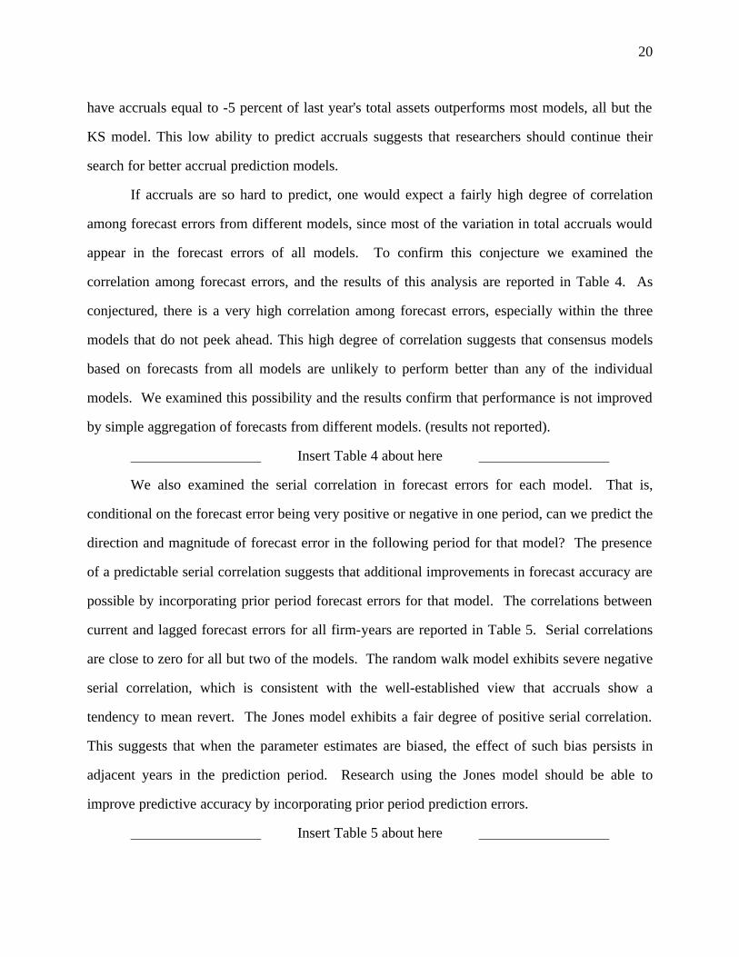
have accruals equal to -5 percent of last year's total assets outperforms most models, all but the

KS model. This low ability to predict accruals suggests that researchers should continue their

search for better accrual prediction models.

If accruals are so hard to predict, one would expect a fairly high degree of correlation

among forecast errors from different models, since most of the variation in total accruals would

appear in the forecast errors of all models. To confirm this conjecture we examined the

correlation among forecast errors, and the results of this analysis are reported in Table 4. As

conjectured, there is a very high correlation among forecast errors, especially within the three

models that do not peek ahead. This high degree of correlation suggests that consensus models

based on forecasts from all models are unlikely to perform better than any of the individual

models. We examined this possibility and the results confirm that performance is not improved

by simple aggregation of forecasts from different models. (results not reported).

Insert Table 4 about here

We also examined the serial correlation in forecast errors for each model. That is,

conditional on the forecast error being very positive or negative in one period, can we predict the

direction and magnitude of forecast error in the following period for that model? The presence

of a predictable serial correlation suggests that additional improvements in forecast accuracy are

possible by incorporating prior period forecast errors for that model. The correlations between

current and lagged forecast errors for all firm-years are reported in Table 5. Serial correlations

are close to zero for all but two of the models. The random walk model exhibits severe negative

serial correlation, which is consistent with the well-established view that accruals show a

tendency to mean revert. The Jones model exhibits a fair degree of positive serial correlation.

This suggests that when the parameter estimates are biased, the effect of such bias persists in

adjacent years in the prediction period. Research using the Jones model should be able to

improve predictive accuracy by incorporating prior period prediction errors.

Insert Table 5 about here

21

5. Extensions

We consider next a series of modifications, primarily to the Jones model, that have been

suggested in prior research. Our objective is to determine if the performance documented so far

can be improved by those modifications.

Beneish (1997, pp. 273) suggests that the Jones model should be expanded to include at

least two additional explanatory variables: lagged total accruals and that year’s market

performance (size-adjusted returns). We estimated firm-specific regressions similar to equation

(9) for the expanded Jones model with the two additional regressors, and examined all four

measures of forecast accuracy considered in Table 3, panels A through D, for the 5-year

prediction period. In general, while the in-sample or prediction period R2 values are substantially

higher for the expanded Jones model, the forecasts are less accurate. For brevity, we only report

(in Panel A of Table 6) comparisons based on the fourth measure of accuracy (R2 relative to a

naïve forecast of –5%). All the R2 values for the expanded Jones model in Table 6, Panel A,

representing the different percentile points are lower than the corresponding points for the Jones

model in Table 3, Panel D. We also provide statistics for the R2 distributions for the other five

models for comparison. Note that the results for the other models differ slightly from those in

Table 3, Panel D, because the final samples are different in the two panels (because of the data

requirements of the expanded Jones model, fewer observations remain in Table 6).

Insert Table 6 about here

The second extension we consider is the impact of updating the model parameters as we

progress through the prediction period. In other words, while the 1975-1989 estimation period is

used for the 1990 forecast, the estimation period is expanded to include 1990 for the 1991

forecast, and so on. Note that this updating procedure has no effect on the random walk and

mean reverting models. Again, while all four sets of accuracy measures were examined, only the

fourth measure is reported in Panel B of Table 6. The results remain essentially unchanged.

Adding additional years does not appear to change the parameter estimates or forecasts

substantially, and there are only slight differences in accuracy, in terms of the percentile points in

22

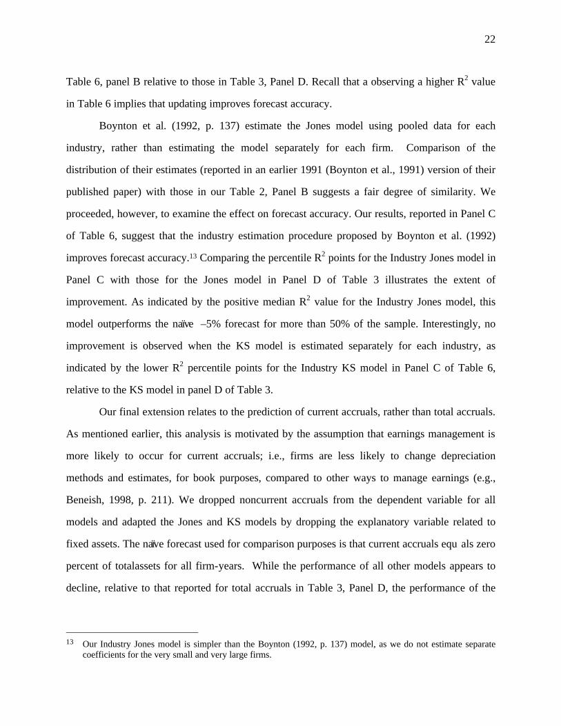
Table 6, panel B relative to those in Table 3, Panel D. Recall that a observing a higher R2 value

in Table 6 implies that updating improves forecast accuracy.

Boynton et al. (1992, p. 137) estimate the Jones model using pooled data for each

industry, rather than estimating the model separately for each firm. Comparison of the

distribution of their estimates (reported in an earlier 1991 (Boynton et al., 1991) version of their

published paper) with those in our Table 2, Panel B suggests a fair degree of similarity. We

proceeded, however, to examine the effect on forecast accuracy. Our results, reported in Panel C

of Table 6, suggest that the industry estimation procedure proposed by Boynton et al. (1992)

improves forecast accuracy.13 Comparing the percentile R2 points for the Industry Jones model in

Panel C with those for the Jones model in Panel D of Table 3 illustrates the extent of

improvement. As indicated by the positive median R2 value for the Industry Jones model, this

model outperforms the naïve –5% forecast for more than 50% of the sample. Interestingly, no

improvement is observed when the KS model is estimated separately for each industry, as

indicated by the lower R2 percentile points for the Industry KS model in Panel C of Table 6,

relative to the KS model in panel D of Table 3.

Our final extension relates to the prediction of current accruals, rather than total accruals.

As mentioned earlier, this analysis is motivated by the assumption that earnings management is

more likely to occur for current accruals; i.e., firms are less likely to change depreciation

methods and estimates, for book purposes, compared to other ways to manage earnings (e.g.,

Beneish, 1998, p. 211). We dropped noncurrent accruals from the dependent variable for all

models and adapted the Jones and KS models by dropping the explanatory variable related to

fixed assets. The naïve forecast used for comparison purposes is that current accruals equ als zero

percent of totalassets for all firm-years. While the performance of all other models appears to

decline, relative to that reported for total accruals in Table 3, Panel D, the performance of the

13 Our Industry Jones model is simpler than the Boynton (1992, p. 137) model, as we do not estimate separate

coefficients for the very small and very large firms.

23

Jones model increases. The median adjusted R2 is close to zero, which suggests that the Jones

model performed better than the naïve model for almost half the sample firms.

Overall, the results in this section suggest that two of the many modifications considered

improve accuracy: a) estimating the Jones model at the industry level (e.g., Boynton et. al., 1992,

p. 137), rather than the firm level, and b) estimating the Jones model for current accruals alone,

rather than total accruals. Despite these improvements, however, the absolute performance is still

not strong, since the naïve models still perform as well or better.

6. Conclusion

Our paper provides some description of accruals and the ability of extant models to

forecast accruals. The following is a brief overview of our findings. Accruals equal about -5

percent of last period's total assets, on average. This mean effect is explained primarily by non-

current accruals (depreciation, depletion and amortization), and current accruals (changes in non-

cash working capital) have a zero mean. Most of the variance in total accruals, however, is

explained by variation in current accruals, with non-current accruals exhibiting much lower

variation. We consider the forecasting ability of three models that peek ahead and use

contemporaneous data to identify unexpected accruals: the Jones, the KS, and Industry models.

We also consider three models that do not peek ahead and use only prior year data: the random

walk model, the mean-reverting model, and a combination model that separates current accruals

from noncurrent accruals and allows each component to follow a different weighted-average of

the random walk and mean-reverting models. Our results indicate low forecasting ability, in

general, for all models.

Despite the many items of information that are input into these models, the performance

of those models is surprising. Researchers seeking to detect earnings management are in effect

using tools that are less accurate than they appear. Simply assuming that total accruals equal -5

percent of total assets outperforms most models. Similarly, assuming that current accruals equal

zero percent of total assets, also outperforms all models when they are adjusted to predict current

24

accruals alone. There are some bright spots, however: we find that the Jones model estimated

separately over different industries and the KS model exhibit some ability to outperform these

naïve expectation models by a small margin.

Also, some of these models tend to overfit within the estimation period, and this

overfitting creates a misplaced sense of security that the models are able to explain some of the

variation in accruals. Ultimately, it is only the explanatory power of the model in out-of-sample

or prediction periods that matters.

25

Appendix Summary of accrual prediction models

1) Random walk Model TOTACCit

TAit-1 =

TOTACCit-1TAit-2

+ eit …(5)

2) Mean-reverting accruals Model TOTACCit

TAit-1 =

15

∑τ=t-5

t-1

TOTACCiτ

TAiτ-1 + eit …(6)

3) Components Model

CURACCit

TAit-1 = (α)

CURACCit-1TAit-2

+ (1-α)

15 ∑

τ=t-5

t-1

CURACCiτ

TAiτ-1 + eit …(7)

NONCURACCit

TAit-1 = (β)

NONCURACCit-1TAit-2

+ (1-β)

15 ∑

τ=t-5

t-1

NONCURACCiτ

TAiτ-1 + eit …(8)

4) Jones Model TOTACCit

TAit-1 = ai

1TAit-1

+ b1i ∆REVitTAit-1

+ b2i PPEitTAit-1

+ eit …(9)

5) Industry Model TOTACCit

TAit-1 = i1i + i2i

industry medianTOTACCit

TAit-1 + eit …(10)

which is estimated over 2-digit SIC industry groups.

6) KS Model

+

+

+=

−

−

−−

−

−−

−

−− 1

1

13

1

1

12

1

1

110

1 t

t

t

t

t

t

t

t

t

t

t

t

t

t

GPPE

DEP

TA

GPPEc

EXP

OCAL

TA

EXPc

REV

ART

TA

REVcc

TA

ACCBAL

and lagged values of the three independent variables are included as instrumental variables. Detailed descriptions of the models can be obtained from the following sources. Random walk model: Dechow et al. (1995, p. 198). Mean-reverting accruals model: Dechow et al. (1995, p. 197) Jones model: Jones (1991, p. 211). Industry model: Dechow et al. (1995, p. 199). KS model: Kang and Sivaramakrishnan (1995, p. 358). The variables are defined as follows (#n refers to Compustat Annual data item #). TOTACC (total accruals) = CURACC + NONCURACC (current + noncurrent accruals) = ∆[(#4−#1) − #5] − #125

26

ACCBAL = noncash current assets and liabilities, (excluding tax receivables and payables) less depreciation = (#4-#1-#161-(#5-#71)-#14 ART = accounts receivable less tax receivables = #2-#161 EXP = expenses = #12-#13 DEP = depreciation from Income Statemen = #14 OCAL = other current assets and liabilities = (#4-ART-#1-#161-(#5-#71) GPPE = gross plant, property and equipment = #7 ΤΑ (Total assets) = #6, REV (Revenues) = #12, PPE (Plant, Property and Equipment) = #7 #4 = current assets, #1 = cash #2 = accounts receivables #5 = current liabilities #12 = sales #13 = operating income before depreciation #71= income taxes payable #125 = depreciation, depletion, and amortization from the cash flow statement #161 = income tax refund

27

Figure 1 Prediction period R2 and pseudo R2 ( 2

aR ) For each sample firm and prediction model, data from the estimation period (1975-1989) are used to estimate the parameters that are needed to make forecasts for the five-year prediction period (1990-1994). Actual accruals in those five years are then plotted against forecast accruals (the five points marked as x). Forecast accuracy is measured by the sum of squared forecast errors, Σ(A-F)2. To convert this measure of accuracy to a conventional R2 value, we examine the fit of the five data points against the 45 degree line on the plot, or the regression line which represents actual accruals=forecast accruals; i.e. the regression line with a slope equal to one and an intercept equal to zero. The forecast errors can thus be represented by the residuals from this regression line, and the sum of squared forecast errors is equal to the conventional error sum of squares (ESS). This error sum of squares is normally compared to the total variation in actual accruals, or total sum of squares (TSS), which is measured by the sum of the squared deviations of the five actual accrual numbers from their mean (µ). The conventional R2 is then equal to 1-ESS/TSS. An R2 value equal to zero suggests that the forecast values perform as well as a naïve constant forecast equal to the mean accrual for all years. Since this mean accrual is not known, we offer a second comparison which

results in a pseudo or adjusted R2 ( 2aR ). Compare the forecasts against a naïve constant forecast equal to –5% for all

firms for all years. This value represents the grand mean for all firms for all years. In other words, compare the ESS against an alternative TSSa, which is the sum of squared deviations of the five actual accrual numbers from –5%.

2

22

)(

)(11

µ−Σ−Σ

−=−=A

FA

TSS

ESSR and

2

22

%))5((

)(11

−−Σ−Σ

−=−=A

FA

TSS

ESSR

aa

Mean of actual accruals=µ

Naïve Model: Forecast = −5%

Actual Accruals

(A)

Forecast Accruals (F)

x x

x

x

x

A=F

28

Table 1

Summary statistics for total accruals and its components 7,195 firm-years (1,748 firms) over the prediction period (1990-1994)

All firm-years between 1990 and 1994 on Compustat with forecasts available for all six accrual prediction models (see appendix for details of models) are included in the sample. Total accruals and its two components are measured as follows. TOTACCit = CURACCit + NONCURACCit = ∆[(#4−#1) − #5] − #125, where data # are from Compustat. All accruals items are scaled by beginning-of-year total assets (TA), which is data item #6. Panel A: Distributional statistics for accrual components.

mean Standard deviation

10th percentile

25th percentile

50th percentile

75th percentile

90th percentile

current accrual -0.02% 10.50% -7.38% -2.95% 0.13% 3.26% 7.38%

noncurrent accrual -5.37% 2.98% -8.91% -6.62% -4.88% -3.51% -2.34%

total accrual -5.39% 10.90% -13.78% -8.99% -5.24% -1.51% 3.11%

Panel B: Correlation among accrual components.* Pearson correlation above main diagonal, and Spearman rank correlation below.

current accrual

noncurrent accrual

Total accrual

current accrual -0.003 0.962

noncurrent accrual -0.013 0.270

total accrual 0.879 0.384

* Correlations greater than 0.023 (0.030) are significant at the 5% (1%) level.

29

Table 2 Parameters estimated for three of the five prediction models

Estimation period (1976-1989) Two of the five models, random walk and mean-reverting accruals, do not require parameter estimates (see appendix for details of models). Parameters for the remaining three models are estimated from all firm-years with available data between 1976 and 1989 on Compustat. Total accruals and its two components are measured as follows. TOTACCit = CURACCit + NONCURACCit = ∆[(#4−#1) − #5] − #125, where data # are from Compustat. All accruals items are scaled by beginning-of-year total assets (TA), which is data item #6. Panel A: Estimated weights from pooled regressions for components model.

CURACCit

TAit-1 = (α)

CURACCit-1TAit-2

+ (1-α)

15 ∑

τ=t-5

t-1

CURACCiτ

TAiτ-1 + eit …(9)

NONCURACCit

TAit-1 = (β)

NONCURACCit-1TAit-2

+ (1-β)

15 ∑

τ=t-5

t-1

NONCURACCiτ

TAiτ-1 + eit …(10)

α = -0.002 from eq. (9), and β = 0.599 from eq. (10), based on 19,943 and 20,966 firm-years. Panel B: Distributional statistics for firm-specific Jones model parameter estimates (2,692 firms with at least 10 years of data).

TOTACCit

TAit-1 = ai

1TAit-1

+ b1i ∆REVitTAit-1

+ b2i PPEitTAit-1

+ eit …(11)

coefficient estimate

mean

standard deviation

10th percentile

25th percentile

50th percentile

75th percentile

90th percentile

ai 7.582 151.512 -8.784 -0.907 0.335 4.632 33.814

b1i 0.068 0.290 -0.161 -0.026 0.071 0.178 0.312

b2i -0.121 0.649 -0.297 -0.151 -0.084 -0.028 0.064

30

Table 2 (continued) Panel C: Distributional statistics for firm-specific Industry model parameter estimates (2,719 firms with at least 10 years of data).

TOTACCit

TAit-1 = i1i + i2i

industry medianTOTACCit

TAit-1 + eit …(12)

coefficient estimate

mean

standard deviation

10th percentile

25th percentile

50th percentile

75th percentile

90th percentile

i1i 0.001 0.118 -0.091 -0.042 -0.002 0.039 0.092

i2i 1.026 2.333 -1.031 0.039 0.909 1.932 3.188

31

Table 3 Forecast accuracy for six accrual prediction models

7,195 firm-years (1,748 firms) over the prediction period (1990-1994) All firm-years between 1990 and 1994 on Compustat with forecasts available for all six accrual prediction models (see appendix for details of models) are included in the sample. Total accruals and its two components are measured as follows. TOTACCit = CURACCit + NONCURACCit = ∆[(#4−#1) − #5] − #125, where data # are from Compustat. All accruals items are scaled by beginning-of-year total assets (TA), which is data item #6.

Panel A: Distributional statistics for forecast errors. Model

mean

Standard deviation

10th percentile

25th percentile

50th percentile

75th percentile

90th percentile

random walk -0.18% 15.17% -11.65% -4.96% -0.30% 4.38% 11.12%

mean reverting -0.65% 11.82% -9.55% -4.25% -0.50% 2.97% 7.80%

components -0.62% 11.83% -9.54% -4.18% -0.44% 2.93% 7.96%

Jones 0.38% 13.65% -9.93% -3.84% 0.47% 4.64% 10.60%

industry -0.69% 11.36% -9.57% -4.24% -0.48% 3.08% 7.98%

KS 0.49% 10.62% -6.59% -2.30% 0.85% 3.99% 8.17%

Panel B: % of times each rank is obtained, based on rankings by firm. model

First Second Third Fourth Fifth Sixth

random walk 7.27% 6.98% 7.72% 10.07% 19.57% 48.40%

mean reverting 7.61% 18.42% 25.17% 26.72% 17.62% 4.46%

components 9.27% 18.65% 25.74% 26.54% 16.08% 3.72%

Jones 17.56% 18.14% 11.67% 10.18% 16.36% 26.09%

industry 21.17% 17.91% 17.33% 14.36% 18.19% 11.04%

KS 37.13% 19.91% 12.36% 12.13% 12.19% 6.29%

32

Table 3 (continued) Forecast accuracy for 6 accrual prediction models

7,195 firm-years (1,748 firms) over the prediction period (1990-1994)

Panel C: Distribution of firm-specific explained variation, (R2=1−−ESS/TSS, where

ESS=ΣΣ(actual-forecast)2 and TSS=ΣΣ(actual−µ−µ)2), where µµ= mean of five actual accruals.

Model

mean

standard deviation

10th percentile

25th percentile

50th percentile

75th percentile

90th percentile

random walk -19.013 404.55 -4.875 -2.595 -1.751 -1.056 -0.523

mean reverting -47.181 1352.41 -2.823 -1.133 -0.529 -0.273 -0.142

components -46.114 1315.77 -2.850 -1.120 -0.495 -0.262 -0.111

Jones -28.489 461.54 -11.604 -3.257 -0.730 -0.107 0.156

industry -10.115 226.69 -4.330 -1.622 -0.476 -0.080 0.058

KS -28.692 798.39 -2.845 -1.016 -0.246 0.074 0.297

Panel D: Distribution of firm-specific explained variation, relative to a naive model of forecast

accrual =−−5% ( 2aR =1−−ESS/TSSa, where ESS=ΣΣ(actual −− forecast)2 and TSSa=ΣΣ(actual −− (−−5%))2)

model

mean

standard deviation

10th percentile

25th percentile

50th percentile

75th percentile

90th percentile

random walk -451.676 15209.68 -3.020 -1.728 -0.811 0.019 0.578

mean reverting -20.623 507.71 -1.204 -0.447 -0.114 0.290 0.683

components -20.616 507.33 -1.223 -0.435 -0.118 0.307 0.707

Jones -332.446 12822.12 -4.227 -1.133 -0.107 0.292 0.622

industry -23.632 814.70 -1.696 -0.508 -0.025 0.316 0.673

KS -412.063 16734.17 -0.959 -0.204 0.135 0.459 0.751

33

Table 4 Correlation among forecast errors from 6 accrual prediction models 7,195 firm-years (1,748 firms) over the prediction period (1990-1994)

All firm-years between 1990 and 1994 on Compustat with forecasts available for all six accrual prediction models (see appendix for details of models) are included in the sample. Total accruals and its two components are measured as follows. TOTACCit = CURACCit + NONCURACCit = ∆[(#4−#1) − #5] − #125, where data # are from Compustat. All accruals items are scaled by beginning-of-year total assets (TA), which is data item #6.

Pearson (Spearman) Correlation above (below) main diagonal.*

model

random walk

mean reverting

components Jones Industry KS

random walk 0.811 0.812 0.609 0.733 0.614

mean reverting 0.728 0.998 0.756 0.903 0.731

components 0.733 0.994 0.755 0.899 0.732

Jones 0.525 0.705 0.699 0.751 0.641

industry 0.598 0.802 0.793 0.677 0.761

KS 0.626 0.746 0.752 0.640 0.701

* Correlations greater than 0.023 (0.030) are significant at the 5% (1%) level.

34

Table 5 Correlation between current and lagged forecast errors from 6 accrual prediction models 7,195 firm-years (1,748 firms) over the prediction period (1990-1994)

All firm-years between 1990 and 1994 on Compustat with forecasts available for all six accrual prediction models (see appendix for details of models) are included in the sample. Total accruals and its two components are measured as follows. TOTACCit = CURACCit + NONCURACCit = ∆[(#4−#1) − #5] − #125, where data # are from Compustat. All accruals items are scaled by beginning-of-year total assets (TA), which is data item #6. Correlation*

random walk

mean reverting

components Jones Industry KS

Pearson -0.527 -0.099 -0.102 0.254 -0.012 0.000

Spearman -0.486 -0.050 -0.060 0.231 0.088 -0.110

* Correlations greater than 0.023 (0.030) are significant at the 5% (1%) level.

35

Table 6 Forecast accuracy for six accrual prediction models

Distribution of firm-specific explained variation, relative to a naive model of forecast accrual =−5%

( 2aR =1−ESS/TSSa, where ESS=Σ(actual − forecast)2 and TSSa=Σ(actual − (−5%))2)

Panel A: Consider expanded Jones model that incorporates prior period accruals and current period size-adjusted returns to the Jones model. Model

mean

standard deviation

10th percentile

25th percentile

50th percentile

75th percentile

90th percentile

random walk -300.201 7191.52 -2.606 -1.698 -0.918 -0.107 0.477

mean reverting -28.833 677.56 -0.977 -0.449 -0.141 0.232 0.616

Components -27.899 656.63 -0.984 -0.429 -0.129 0.254 0.625

Expanded Jones -12.016 150.16 -6.564 -2.162 -0.423 0.176 0.538

Industry -11.697 256.06 -1.279 -0.430 -0.024 0.281 0.638

KS -32.019 765.75 -0.810 -0.175 0.121 0.399 0.670

Panel B: Consider updated models that update the parameters using prior years from the prediction period. Model

mean

standard deviation

10th percentile

25th percentile

50th percentile

75th percentile

90th percentile

random walk -388.533 13954.84 -3.639 -1.765 -0.789 0.076 0.651

mean reverting -21.274 476.32 -1.448 -0.482 -0.104 0.329 0.706

updated components

-24.755 586.38 -1.456 -0.480 -0.095 0.340 0.723

updated Jones -32.994 905.44 -4.391 -1.017 -0.169 0.303 0.665

updated industry -5.888 147.04 -1.761 -0.485 -0.066 0.323 0.697

updated KS -363.992 16015.66 -1.307 -0.236 0.145 0.497 0.781

36

Table 6 (continued) Forecast accuracy for six accrual prediction models

Distribution of firm-specific explained variation, relative to a naive model of forecast accrual =−5%

( 2aR =1−ESS/TSSa, where ESS=Σ(actual − forecast)2 and TSSa=Σ(actual − (−5%))2)

Panel C: Consider industry Jones model that estimates the Jones model over the prior 5 years separately for each 2-digit SIC industry. model

Mean

Standard deviation

10th percentile

25th percentile

50th percentile

75th percentile

90th percentile

random walk -388.350 13951.48 -3.657 -1.767 -0.794 0.073 0.650

mean reverting -21.264 476.21 -1.448 -0.482 -0.103 0.327 0.706

components -24.743 586.24 -1.456 -0.480 -0.095 0.339 0.723

industry Jones -100.707 4234.91 -2.317 -0.522 0.004 0.345 0.635

industry -5.887 147.00 -1.767 -0.485 -0.068 0.322 0.696

industry KS -748.389 33291.58 -3.902 -0.804 0.022 0.411 0.732

Panel D: Use the six standard models to predict current accruals, rather than total accruals. The naïve forecast used is current accruals=0% for all firm -years. model

Mean

Standard deviation

10th percentile

25th percentile

50th percentile

75th percentile

90th percentile

random walk -11.954 246.08 -3.575 -2.011 -1.262 -0.443 0.174

mean reverting -14.599 566.05 -1.379 -0.550 -0.238 -0.007 0.250

components -14.631 567.39 -1.404 -0.549 -0.237 -0.007 0.251

Jones -4.609 86.81 -1.327 -0.300 -0.002 0.186 0.458

industry -11.794 400.24 -1.817 -0.546 -0.095 0.097 0.369

KS -6.481 126.07 -1.743 -0.529 -0.045 0.231 0.514

37

References

Bartov, E., 1993. The timing of asset sales and earnings manipulation. The Accounting Review

68 (4), 840 – 855.

Beneish, M.D., 1997. Detecting GAAP violation: implications for assessing earnings

management among firms with extreme financial performance. Journal of Accounting and

Public Policy 16 (3), 271 – 309.

Beneish, M.D., 1998a. A call for papers: Earnings mangement. Journal of Accoutning and

Public Policy 17 (1), 85-88.

Beneish, M.D., 1998b. Discussion of “Are Accruals during Initial Public Offerings

Opportunistic.” Review of Accounting Studies 3 (1, 2), 209-221.

Boynton, C., Dobbins, P., Plesko, G., 1991. Earnings management and the corporate alternative

minimum tax. Working paper, University of North Texas, Denton, TX.

Boynton, C., Dobbins, P., Plesko, G., 1992. Earnings management and the corporate alternative

minimum tax. Journal of Accounting Research 30 (Supplement), 131 – 153.

Choi, W., Gramlich, J., Thomas, J., 1997. Did firms decrease book income in 1987 to reduce the

AMT impact? The case against. Working paper, Columbia Business School, Columbia

University, New York, NY.

Dhaliwal, D., Salamon, G., Smith, E., 1982. The effect of owner versus management control on

the choice of accounting methods. Journal of Accounting and Economics 4 (1), 41 – 53.

DeAngelo, H., DeAngelo, L., Skinner, D., 1994. Accounting choice in troubled companies.

Journal of Accounting and Economics 17 (1, 2), 113 – 143.

DeAngelo, L., 1986. Accounting numbers as market valuation substitutes: A study of

management buyouts of public stockholders. The Accounting Review 61 (3), 400 – 420.

DeAngelo, L., 1988. Managerial competition, information costs, and corporate governance, the

use of accounting performance measures in proxy contests. Journal of Accounting and

Economics 10 (1), 3 – 36.

38

Dechow, P., 1994. Accounting earnings and cash flows as measures of firm performance: The

role of accounting accruals. Journal of Accounting and Economics 18 (1), 3 – 42.

Dechow, P., Sloan, R., Sweeney, A., 1995. Detecting earnings management. The Accounting

Review 70 (2), 193 – 225.

DeFond, M., Jiambalvo, J., 1994. Debt covenant violation and manipulation of accruals. Journal

of Accounting and Economics 17 (1,2), 145 – 176.

Gaver, J., Gaver, K., Austin, J., 1995. Additional evidence on bonus plans and income

management. Journal of Accounting and Economics 19 (1), 3 – 28.

Guay, W., Kothari, S.P., Watts, R., 1996. A market-based evaluation of discretionary-accrual

models. Journal of Accounting Research 34 (Supplement), 83 – 105.

Guenther, D., 1994. Earnings management in response to corporate tax rate changes: Evidence

from the 1986 tax reform act. The Accounting Review 69 (1), 230 – 243.

Healy, P., 1985. The effect of bonus schemes on accounting decisions. Journal of Accounting

and Economics 7 (1-3), 85 – 107.

Healy, P., 1996. Discussion of “A Market-Based Evaluation of Discretionary Accrual Models.”

Journal of Accounting Research 34 (Supplement), 107 – 115.

Holthausen, R., Larcker, D., Sloan, R., 1995. Annual bonus schemes and the manipulation of

earnings. Journal of Accounting and Economics 19 (1), 29 – 74.

Jones, J., 1991. Earnings management during import relief investigations. Journal of Accounting

Research 29 (2), 193 – 228.

Kang, S., 1999. Earnings management to avoid losses and performance of accrual prediction

models. Working paper, Yale School of Management, New Haven, CT.

Kang, S., Sivaramakrishnan, K., 1995. Issues in testing earnings management and an

instrumental variable approach. Journal of Accounting Research 33 (2), 353 – 367.

McNichols, M., Wilson, G., 1988. Evidence of earnings management from the provision for bad

debts. Journal of Accounting Research 26 (Supplement), 1 – 31.

39

Miller, G., Skinner, D., 1998. Determinants of the valuation allowance for deferred tax assets

under SFAS-109. The Accounting Review 73 (2), 213 – 233.

Perry, S., Williams, T., 1994. Earnings management preceding management buyout offers.

Journal of Accounting and Economics 18 (2), 157 – 179.

Pourciau, S., 1993. Earnings management and nonroutine executive changes. Journal of

Accounting and Economics 16 (1-3), 317 – 336.

Schipper, K., 1989. Earnings management. Accounting Horizons 1989 (December), 91-102.

Skinner , D., 1993. The investment opportunity set and accounting procedure choice: Preliminary

evidence. Journal of Accounting and Economics 16 (4), 407 – 445.

Sloan, R., 1996. Do stock prices fully reflect information in accruals and cash flows about future

earnings? The Accounting Review 71 (3), 289 – 315.

Subramanyam, K.R., 1996. The pricing of discretionary accruals. Journal of Accounting and

Economics 19 (1-3), 249 – 281.

Watts, R., Zimmerman, J., 1986. Positive Accounting Theory. Prentice-Hall, Inc., Englewood

Cliffs, New Jersey.