iee proceedings review copy only - missouri university …web.mst.edu/~autosys/papers/008.pdfoptimal...

Optimal Dynamic Inversion Control Design for a Class of Nonlinear Distributed Parameter Systems with Continuous and Discrete Actuators

Journal: IEE Proc. Control Theory & Applications Manuscript ID: draft

Manuscript Type: Research Paper Date Submitted by the

Author: n/a

Complete List of Authors: Padhi, Radhakant; Indian Institute of Science, Aerospace Engineering Balakrishnan, S.N.; University of Missouri-Rolla, Aerospace Engineering

Keyword: Optimal dynamic inversion, DISTRIBUTED PARAMETER SYSTEMS, TEMPERATURE CONTROL

IEE Proceedings Review Copy Only

Control Theory & Applications

Optimal Dynamic Inversion Control Design for a Class of Nonlinear

Distributed Parameter Systems with Continuous and Discrete Actuators

Radhakant Padhi 1 and S. N. Balakrishnan 2

1Department of Aerospace Engineering, Indian Institute of Science – Bangalore, India 2Department of Mechanical and Aerospace Engineering, University of Missouri – Rolla, USA

Abstract

Combining the principles of dynamic inversion and optimization theory, two stabilizing state

feedback control design approaches are presented for a class of nonlinear distributed parameter systems.

One approach combines the dynamic inversion with variational optimization theory and it can be applied

when there is a continuous actuator in the spatial domain. This approach has more theoretical significance

in the sense that the convergence of the controller can be proved and it does not lead to any singularity in

the control computation as well. The other approach, which can be applied when there are a number of

discrete actuators located at distinct places in the spatial domain, combines dynamic inversion with static

optimization theory. This approach has more relevance in practice, since such a scenario appears naturally

in many practical problems because of implementation concern. These new techniques can be classified

as “design-then-approximate” techniques, which are in general more elegant than the “approximate-then-

design” techniques. However, unlike the existing design-then-approximate techniques, the new

techniques presented here do not demand involved mathematics (like infinite dimensional operator

theory). To demonstrate the potential of the proposed techniques, a real-life temperature control problem

for a heat transfer application is solved, first assuming a continuous actuator and then assuming a set of

discrete actuators.

Keywords: Dynamic inversion, Optimal dynamic inversion, Distributed parameter systems,

Temperature control, Design-then-approximate

1 Asst. Professor, Email: [email protected] , Tel: +91-80-2293-2756, Fax: +91-80-2360-0134 2 Professor, Email: [email protected], Tel: +1-573-341-4675, Fax: +1-573-341-4607

Page 1 of 25



2

1. Introduction

There are wide class of problems (e.g. heat transfer, fluid flow, flexible structures etc.)

for which a lumped parameter modeling is inadequate and a distributed parameter system (DPS)

approach is necessary. Control design for distributed parameter systems is often more

challenging as compared to lumped parameter systems and it has been studied both from

mathematical as well as engineering point of view. An interesting brief historical perspective of

the control of such systems is found in [Lasiecka]. In a broad sense, existing control design

techniques for distributed parameter systems can be attributed to either “approximate-then-

design (ATD)” or “design-then-approximate (DTA)” categories. An interested reader can refer to

[aBurns] for discussions on the relative merits and limitations of the two approaches.

In the ATD approach the idea is to first come up with a low-dimensional reduced

(truncated) model, which retains the dominant modes of the system. This truncated model (which

is often a finite-dimensional lumped parameter model) is then used to design the controller. One

such potential approach, which has become fairly popular, first comes up with problem-oriented

basis functions using the idea of proper orthogonal decomposition (POD) (through the “snap-

shot solutions”) and then uses those in a Galerkin procedure to come up with a low-dimensional

reduced lumped parameter approximate model (which usually turns out to be a fairly good

approximation). Out of numerous literatures published on this topic and its use in control system

design, we cite [Annaswamy, Arien, Banks, bBurns, Christofides, Holmes, Padhi, Ravindran,

Singh] for reference. For linear systems, such an approach of designing the POD based basis

function leads to the optimal representation of the PDE system in the sense that it captures the

maximum energy of the system with least number of basis functions as compared to any other set

of orthogonal basis functions [Holmes]. For nonlinear systems, however, such a useful result

does not exist.

Even though the POD based model reduction idea has been successfully used for

numerous linear and nonlinear DPS in both linear as well as nonlinear problems, there are a few

important shortcomings in the POD approach: (i) the technique is problem dependent and not

generic; (ii) there is no guarantee that the snap-shot solutions will capture all dominant modes of

the system and, most important, (iii) it is usually difficult to have a set of ‘good’ snap-shot

Page 2 of 25



3

solutions for the closed-loop system prior to the control design. This is a serious limiting factor

for applying this technique in the closed-loop control design. Because of this reason, some

attempts are being made in recent literature to adaptively redesign the basis functions (and hence

the controller) in an iterative manner. An interested reader can see [Annaswamy, Arien,

Ravindran] for a few ideas in this regard.

In the DTA approach, on the other hand, the usual procedure is to use infinite

dimensional operator theory to come up with the control design in the infinite dimensional space

first [Curtain]. For implementation purpose, this controller is then approximated to a finite

dimensional space by truncating an infinite series, reducing the size of feedback gain matrix etc.

An important advantage of this approach is that it takes into account the full system dynamics in

designing the controller, and hence, usually performs better [aBurns]. However, to the best of the

knowledge of the authors, these operator theory based DTA approaches are mainly limited to

linear distributed parameter systems [Curtain] and some limited class of problems like spatially

invariant systems [Bameih]. Moreover the mathematics of the infinite dimensional operator

theory is usually involved, which is probably another reason why it has not been able to become

popular among practicing engineers. One of the main contributions of this paper is that it

presents two generic control design approaches for a class of nonlinear distributed parameter

systems, which are based on the DTA philosophy. Yet they are fairly straightforward, quite

intuitive and reasonably simple, making it easily accessible to practicing engineers. The only

approximation needed here is rather the spatial grid size selection for the control

computation/implementation (which can be quite small, since the computational requirements

are very minimal).

In the control design literature for lumped parameter systems, a relatively simple,

straightforward and reasonably popular method of nonlinear control design is the technique of

dynamic inversion (e.g. [Enns], [Lane], [Ngo]), which is essentially based on the philosophy of

feedback linearization [Slotine]. In this approach, first an appropriate coordinate transformation

is carried out to make the system dynamics take a linear form (in the transformed coordinates).

Then linear control design tools are used to synthesize the controller. Even though the idea

sounds elegant, it turns out that this method is quite sensitive to modeling and parameter

inaccuracies, which has been a potential limiting factor for its usage in practical applications for

Page 3 of 25



4

quite some time. However, a lot of research has been carried out in the recent literature to

address this critical issue. One way of addressing the problem is to augment the dynamic

inversion technique with the H∞ robust control theory [Ngo]. Another way is to augment this

control with neural networks (trained online) so that the inversion error is cancelled out for the

actual system ([Kim], [McFarland]). With the availability of these augmenting techniques,

dynamic inversion has evolved as a potential nonlinear control design technique.

Using the fundamental idea of dynamic inversion and combining it with the variational

and static optimization theories [Bryson], two formulations are presented in this paper for

designing the control system for one-dimensional control-affine nonlinear distributed parameter

systems. We call this merger as “optimal dynamic inversion” for obvious reasons. Out of the two

techniques presented here, one assumes a continuous actuator in the spatial domain (we call this

as ‘continuous controller’). The other technique assumes a number of actuators located at

discrete locations in the spatial domain (which we call as a ‘discrete controller’). The continuous

controller formulation has a better theoretical significance in the sense that the convergence of

the controller to its steady-state profile can be proved with the evolution of time. In the process,

unlike the discrete controller formulation, it does not lead to any singularity in the required

computations either. On the other hand, the discrete controller formulation has more relevance in

practice in the sense that such a scenario appears naturally in many (probably all) practical

problems (a continuous controller is probably never realizable). To demonstrate the potential of

the proposed techniques, a real-life temperature control problem for a heat transfer application is

solved, applying both the continuous as well as the discrete control design ideas.

A few salient points with respect to the new techniques presented here are as follows.

First, even though the optimization idea is used, the new approach is fundamentally different

from optimal control theory. The main driving idea here is rather dynamic inversion, which

guarantees stability of the closed loop (the rate of decay of the error rather depends on the

selected gain matrix and not on the cost function weights). In addition, this objective is achieved

with a minimum control effort (in a weighted 2L or 2l norm sense), where the cost function

plays an important role in the sense that it not only leads to a minimum control effort, but also

distributes the task among various available controllers (which are located at different locations

in the spatial domain). Second, the technique leads to a state feedback control solution in closed

Page 4 of 25



5

form (hence, unlike optimal control theory, it does not demand any computationally intensive

procedure in the control computation). Finally, even though they can be classified into DTA

category, the techniques presented do not demand the knowledge of complex mathematical tools

like infinite dimensional operator theory. Hence, we hope that the techniques will be quite useful

to practicing engineers.

2. Problem Description

2.1 System Dynamics with Continuous Controller

In the continuous controller formulation, we consider the following system dynamics

( ) ( ), , , ... , , , ...x f x x x g x x x u′ ′′ ′ ′′= + (1)

where the state ( ),x t y and controller ( ),u t y are continuous functions of time 0t ≥ and spatial

variable [ ]0,y L∈ . x represents /x t∂ ∂ and ,x x′ ′′ represent /x y∂ ∂ , 2 2/x y∂ ∂ respectively. We

assume that appropriate boundary conditions (e.g. Dirichlet, Neumann etc.) are available to make

the system dynamics description Eq.(1) complete. Both ( ),x t y and ( ),u t y are considered to be

scalar functions. The control variable appears linearly, and hence, the system dynamics is in the

control affine form. Furthermore, we assume that the function ( ), , , ...g x x x′ ′′ is bounded away

from zero, i.e. ( ), , , ... 0 ,g x x x t y′ ′′ ≠ ∀ . In this paper, we do not take into account those

situations where control action enters the system dynamics through the boundary actions (i.e.

boundary control problems are not considered).

2.2 System Dynamics with Discrete Controllers

In the discrete controller formulation, we assume that a set of discrete controllers mu are

located at my ( 1, ,m M= ) locations, with the following assumptions:

• The width of the action of the controller located at my is mw .

Page 5 of 25



6

• In the interval [ ] [ ]/ 2, / 2 0,m m m my w y w L− + ⊂ , the controller ( ),mu t y is assumed to have

a constant magnitude. Outside this interval, 0mu = . However, the interval mw may or

may not be small.

• There is no overlapping of the controller located at my with its neighboring controllers.

• No controller is placed exactly at the boundary, i.e. the control action does not affect the

system through boundary actions.

For this case the system dynamics can be written as follows

( ) ( )1

, , , , , ,M

mm

x f x x x g x x x u=

′ ′′ ′ ′′= +∑ (2)

2.3 Goal for the Controller

The goal for the controller in both continuous and discrete actuator cases is same; i.e. the

controller should make sure that the state variable ( ) ( )*, ,x t y x t y→ as t →∞ for all [ ]0,y L∈ ,

where ( )* ,x t y is a known (possibly time-varying) profile in the domain [ ]0, L , which is

continuous in y and satisfies the spatial boundary conditions.

3. Synthesis of the Controllers

3.1 Synthesis of Continuous Controller

First, we define an output (an integral error) term as follows

( ) ( ) ( ) 2*

0

1 , ,2

Lz t x t y x t y dy = − ∫ (3)

Note that when ( ) 0z t → , ( ) ( )*, ,x t y x t y→ everywhere in [ ]0,y L∈ . Next, following the

principle of dynamic inversion [Enns, Lane, Ngo, Slotine], we attempt to design a controller such

that the following stable first-order equation (in time) is satisfied

Page 6 of 25



7

0z k z+ = (4)

where, 0k > serves as a gain; an appropriate value of k has to be chosen by the control

designer. To have a better physical interpretation, one may choose ( )1/k τ= , where 0τ > serves

as a “time constant” for the error ( )z t to decay. Using the definition of z from Eq.(3), Eq.(4)

leads to

( )( ) ( )2* * *

0 02L Lkx x x x dy x x dy− − = − −∫ ∫ (5)

Substituting for x from Eq.(1) in Eq.(5) and simplifying we arrive at

( ) ( )

( ) ( ) ( )

*

02

* * *

0 0

, , , ...

where , , , ...2

L

L L

x x g x x x u dy

kx x f x x x x dy x x dy

γ

γ

′ ′′− =

′ ′′ − − − − −

∫

∫ ∫ (6)

Note that the value for ( ),u t y satisfying Eq.(6) will eventually guarantee that ( ) 0z t →

as t →∞ . However, since Eq.(6) is in the form of an integral, there is no unique solution can be

obtained for ( ),u t y from it. To obtain a unique solution, however, we have the freedom of

putting an additional goal. We take advantage of this fact and aim to obtain a solution for ( ),u t y

that will not only satisfy Eq.(6), but at the same time, will also minimize the cost function

( ) ( ) 2

0

1 ,2

LJ r y u t y dy= ∫ (7)

In other words, we wish to minimize the cost function in Eq.(7), subjected to the constraint in

Eq.(6). An implication of choosing this cost function is that the aim is to obtain the control

solution ( ),u t y that will lead to ( ) ( )*, ,x t y x t y→ with minimum control effort. In Eq.(7),

( ) [ ]0, 0,r y y L> ∈ is the weighting function, which needs to be chosen by the control

designer. This weighting function gives the designer the flexibility of putting relative importance

of the control magnitude at different spatial locations. Note that the choice of

Page 7 of 25



8

( ) [ ]0,r y c y L+= ∈ ∀ ∈R means the control magnitude is given equal importance at all spatial

locations.

Following the technique for constrained optimization [Bryson], we first formulate the

following augmented cost function

( )2 *

0 0

12

L LJ r u dy x x g u dyλ γ = + − − ∫ ∫ (8)

where λ is a Lagrange multiplier, which is a free variable needed to convert the constrained

optimization problem to a free optimization problem. In Eq.(8), we have two free variables,

namely u and λ . We have to minimize J by appropriate selection of these variables.

The necessary condition of optimality is given by [Bryson]

0Jδ = (9)

where Jδ represents the first variation of J . However, we know that

[ ] ( ) ( )

( ) ( )

* *

0 0 0

* *

0 0

L L L

L L

J ru u dy x x g u dy x x g u dy

ru x x g u dy x x g u dy

δ δ λ δ δλ γ

λ δ δλ γ

= + − + − − = + − + − −

∫ ∫ ∫

∫ ∫ (10)

From Eqs.(9) and (10), we obtain

( ) ( )* *

00

Lru x x g u dy x x g u dyλ δ δλ γ + − + − − = ∫ (11)

Since Eq.(11) must be satisfied for all variations uδ and δλ , the followings equations should be

satisfied simultaneously

( )* 0ru x x gλ+ − = (12)

( )*

0

Lx x g u dy γ− =∫ (13)

Page 8 of 25



9

Note that Eq.(13) is nothing but Eq.(6a). Solving for u from Eq.(12) we get

( )( )*/u r x x gλ= − − (14)

Substituting the above expression for u in Eq.(13) and solving for λ we get

( )2* 2

0

L x x gdy

r

γλ −=

−∫

(15)

Substituting this expression for λ back in Eq.(14), we finally obtain

( )

( ) ( )( )

*

2* 2

0

L

x x gu

x x gr y dy

r y

γ −=

−∫

(16)

As a special case, if ( )r y c += ∈ (i.e. equal weightage is given to the controller at all spatial

locations) and ( ), , , ...g x x x β′ ′′ = ∈R , then Eq.(16) simplifies to

( )( )

*

2*

0

L

x xu

x x dy

γ

β

−=

−∫ (17)

It may be noticed that when ( ) ( )*, ,x t y x t y= (i.e. perfect tracking occurs), there is some

computational difficulty in the sense that a zero seems to appear in the denominator of Eqs.(16-

17), which leads to singularity in the control solution u , i.e. u →∞ . However, even though this

seems to be obvious, it does not happen. To see this, we will show that when ( ) ( )*, ,x t y x t y→ ,

( ) ( )*, ,u t y u t y→ , where ( )* ,u t y is defined as the control required to keep ( ),x t y at ( )* ,x t y

(see Eq.(19)). Before showing this, however, we need a non-trivial expression for ( )* ,u t y . For

that, when ( ) ( )*, ,x t y x t y→ , [ ]0,y L∀ ∈ , from Eq.(1) that we can write

Page 9 of 25



10

( ) ( )* * * *

* * * * * * * *where , , , , , , ,

x f g u

f f x x x g g x x x

= +

′ ′′ ′ ′′ (18)

From Eq.(18), we can write the control solution as

( )* * **

1,u t y f xg

= − − (19)

Note that the solution ( )* ,u t y in Eq.(19) will always be of finite magnitude, since for the

class of DPS considered here, ( )* * * *, , ,g g x x x′ ′′= is always bounded away from zero. Also

note that in actual implementation of the controller, we may rarely encounter the condition

( ) ( ) [ ]*, , 0,x t y x t y y L= ∀ ∈ , since it is very difficult to meet. However, this expression is useful

in the convergence analysis of the controller. Next, we state and prove the following

convergence result.

Theorem

( ),u t y in Eq.(16) converges to ( )* ,u t y in Eq.(19) when ( ) ( ) [ ]*, , 0,x t y x t y y L→ ∀ ∈ .

Proof:

First we notice that at any point ( )0 0,y L∈ , the control solution in Eq.(16) can be written as

( )( ) ( ) ( ) ( ) ( ) ( ) ( ) ( ) ( )

( )( ) ( ) ( )

( )

2* * * *0 0 0 0 0

0 2 2*

0 0

2L L

L

kx y x y g y x y x y f y x y dy x y x y dyu y

x y x y g yr y dy

r y

− − − − + − = −

∫ ∫

∫

(20)

We want to analyze this solution for the case when ( ) ( )*, ,x t y x t y= for all [ ]0,y L∈ .

Without loss of generality, we analyze the case in the limit when ( ) ( )*, ,x t y x t y→ , for

[ ] [ ]0 0/ 2, / 2 0, , 0y y y Lε ε ε∈ − + ⊂ → and ( ) ( )*, ,x t y x t y= everywhere else. In such a

limiting case, let us denote ( )0,u t y as ( )0,u t y , which is given by

Page 10 of 25



11

( )( ) ( ) ( ) ( ) ( ) ( ) ( ) ( ) ( )

( )( ) ( ) ( )

( )

( ) ( ) ( ) ( ) ( ) ( )

0 0

0 0

0

0

2* * * *2 20 0 0

2 20 2 2*

2

2

* * *0 0 0 0 0 0

, , , , , , , , ,2

,, , ,

, , , , , ,

y y

y y

y

y

kx t y x t y g t y x t y x t y f t y x t y dy x t y x t y dyu t y

x t y x t y g t yr y dy

r y

x t y x t y g t y x t y x t y f t y x

ε ε

ε ε

ε

ε

+ +

− −

+

−

− − − − + − = −

− − − − =

∫ ∫

∫

( ) ( ) ( )

( )( ) ( ) ( )

( )

( ) ( ) ( )

( )

2*0 0 0

2 2*0 0 0

00

*0 0

0

*0

, , ,2

, , ,

1 , ,,

,

kt y x t y x t y

x t y x t y g t yr y

r y

f t y x t yg t y

u t y

ε ε

ε

+ − −

− = −

=

(21)

Moreover, this happens ( )0 0,y L∀ ∈ . Hence ( ) ( ) ( ) ( )* *, , as , ,u t y u t y x t y x t y→ → , [ ]0,y L∀ ∈ .

This completes the proof.

Final Control Solution for Implementation

Combining the results in Eqs.(16) and (17), we finally write the control solution as

( ) ( ) [ ]

( )

( ) ( )( )

* * **

**

2* 2

0

1 , if , , 0,

, otherwiseL

f x x t y x t y y Lg

x x gu

x x gr y dy

r y

γ

− − = ∀ ∈ −= −

∫

(22)

Even though ( ) ( )*, ,u t y u t y→ when ( ) ( ) [ ]*, , 0,x t y x t y y L→ ∀ ∈ , in the numerical

implementation of the controller, it is advisable to exercise the caution as outlined in Eq.(22) to

avoid numerical problems in computer programming.

One can notice in the development of Eq.(22) that there was no need of approximating

the system dynamics to come up with the closed form control solution. However, to

compute/implement the control, there is a requirement for choosing a suitable grid in the spatial

domain. Hence, the technique proposed can be classified into the ‘design-then-approximate’

category. Note that a finer grid can be selected to compute ( )* ,u t y since the only computation

that depends on the grid size in Eq.(22) is a numerical integration, which does not demand

intensive computations.

Page 11 of 25



12

3.2 Synthesis of Discrete Controllers

In this section we concentrate on the case when we have only a set of discrete controllers

(as described in Section 2.2). In such a case, following the development in continuous

formulation (Section 3.1), we arrive at the following equation

( ) ( ) ( )*

01

, , , ... ,ML

m m mm

x x g x x x u y w dy γ=

′ ′′− =∑∫ (23)

where γ is as defined in Eq.(6b). Expanding Eq.(23), we can write

( ) ( )1

1

11

* *2 21

2 2

MM

MM

w wy y

w w My yx x g dy u x x g dy u γ

+ +

− −

− + + − =

∫ ∫ (24)

For convenience, we define

( )*2

2

, 1, ,m

m

mm

wy

wm yI x x g dy m M

+

−− =∫ … (25)

Then from Eqs.(24) and (25), we can write

1 1 M MI u I u γ+ + = (26)

Eq.(26) will eventually guarantee that ( ) 0z t → as t →∞ . However, note that Eq.(26) is

a single equation with M variables , 1, ,mu m M= … and hence we have infinitely many

solutions. To obtain a unique solution, we aim to obtain a solution that will not only satisfy

Eq.(26), but at the same time will also minimize the following cost function

( )2 21 1 1

12 M M MJ r w u r w u= + + (27)

In other words, we wish to minimize the cost function in Eq.(27), subjected to the constraint in

Eq.(26). An implication choosing this cost function is that we wish to obtain the solution that

will lead to minimum control effort. In Eq.(27), choosing appropriate values for 1, , 0Mr r >…

Page 12 of 25



13

gives a control designer the flexibility of putting relative importance of the control magnitude at

different spatial locations my , 1, ,m M= … .

Following the principle of constrained optimization [Bryson], we first formulate the

following augmented cost function

( ) ( )2 21 1 1 1 1

1 ...2 M M M M MJ r w u r w u I u I uλ γ= + + + + + − (28)

where λ is a Lagrange multiplier, which is a free variable needed to convert the constrained

optimization problem to a free optimization problem. In Eq.(28) we have λ and

, 1, ,mu m M= … as free variables, with respect to which the minimization has to be carried out.

The necessary condition of optimality [Bryson] leads to the following equations

0, 1, ,m

J m Mu∂

= =∂

… (29)

0Jλ∂

=∂

(30)

Expanding Eqs.(29) and (30) leads to

0, 1, ,m m m mr w u I m Mλ+ = = … (31)

1 1 M MI u I u γ+ + = (32)

Solving for 1, , Mu u… from Eq.(31), substituting those in Eq.(32) and solving for λ we get

( )2

1

/M

m m mm

I r w

γλ

=

−=

∑ (33)

Eqs.(31) and (33) lead to the following expression

Page 13 of 25



14

( )2

1

/

mm M

m m m m mm

Iur w I r w

γ

=

=

∑, 1, ,m M= … (34)

As a special case, when 1 Mr r= = (i.e. equal important to minimization of all controllers) and

1 Mw w= = (i.e. widths of all controllers are same), we have

22

mm

IuIγ

= (35)

where [ ]1T

MI I I . Note that in case we have a number of controllers being applied over

different control application widths (i.e. , 1, ,mu m M= … are different), we can still use the

simplified formula in Eq.(35), if it leads to satisfactory system response by choosing 1, , Mr r

such that 1 1 M Mr w r w= = .

Singularity in Control Solution and Revised Goal:

From Eqs.(34) and (35), it is clear that when 22 0I → (which happens when all of

1, , 0MI I →… ) and 0γ → , there is a problem of singularity in the control computation in the

sense that mu →∞ (this happens since the denominators of Eqs.(34-35) go to zero faster than the

corresponding numerators). Note that if the number of controllers M is large, probably the

occurrence of such a singularity is a rare possibility, since all of 1, , 0MI I →… simultaneously is

rather a strong condition. Nevertheless such a case may arise during transition. More important,

this issue of control singularity will always arise when ( ) ( )*, ,x t y x t y→ , [ ]0,y L∀ ∈ (which is

the primary goal of the control design). This happens possibly because we have only limited

control authority (controllers are available only in a subset of the spatial domain), whereas we

have aimed to achieve a much bigger goal of tracking the state profile [ ]0,y L∀ ∈ - something

that is beyond the capability of the controllers. Hence whenever such a case arises (i.e. when all

of 1, , 0MI I →… or, equivalently, 2 0I → ), to avoid the issue of control singularity, we

propose to redefine the goal as follows.

Page 14 of 25



15

First, we define [ ]1, , TMX x x , * * *

1 , ,M

TX x x and the error vector ( )*E X X− . Next,

we aim to design a controller such that 0E → as t →∞ . In other words, we aim to guarantee

that the values of the state variable at the node points ( , 1, ,my m M= … ) track their

corresponding desired values. We do this, we select a positive definite gain matrix K such that:

0E K E+ = (36)

One way of selecting such a gain matrix K is to choose it a diagonal matrix with thm diagonal

element being ( )1/m mk τ= where 0mτ > is the desired time constant of the error dynamics. In

such a case, the thm channel of Eq.(36) can be written as

0m m me k e+ = (37)

Expanding the expressions for me and me and solving for mu ( 1, ,m M= … ), we obtain

( )* *1m m m m m m

m

u x f k x xg

= − − − (38a)

where ( ),m mx x t y , ( )* * ,m mx x t y , ( ),m mf f t y , ( ),m mg g t y (38b)

Final Control Solution for Implementation

Combining the results in Eqs.(34) and (38), we finally write the control solution as

( )

( )

* *2

2

1

1 , if

, otherwise/

m m m m mm

m mM

m m m m mm

x f k x x I tolg

u I

r w I r w

γ

=

− − − < =

∑

(39)

where tol represents a tolerance value. An appropriate value for this tuning variable can be fixed

by the control designer. Note that some discontinuity/jump in the control magnitude is expected

when the switching takes place. However, this jump can be minimized by judiciously selecting a

proper tolerance value.

Page 15 of 25



16

One can notice that there was no need of approximating the system dynamics (like

reducing it to a low-order lumped parameter model) to come up with the closed form control

solution in Eq.(39). However, like the continuous controller formulation, to compute/implement

the control, there is a requirement for choosing a suitable grid in the spatial domain. Hence, this

technique can also be classified into the ‘design-then-approximate’ category. In this case too, a

finer grid can be selected to compute , 1, ,mu m M= since the only computation that depends

on the grid size in Eq.(39) is a series of numerical integrations, which do not demand intensive

computations.

4. A Motivating Nonlinear Problem

4.1 Mathematical Model

The problem used to demonstrate the theories presented in Section 3 is a real-life

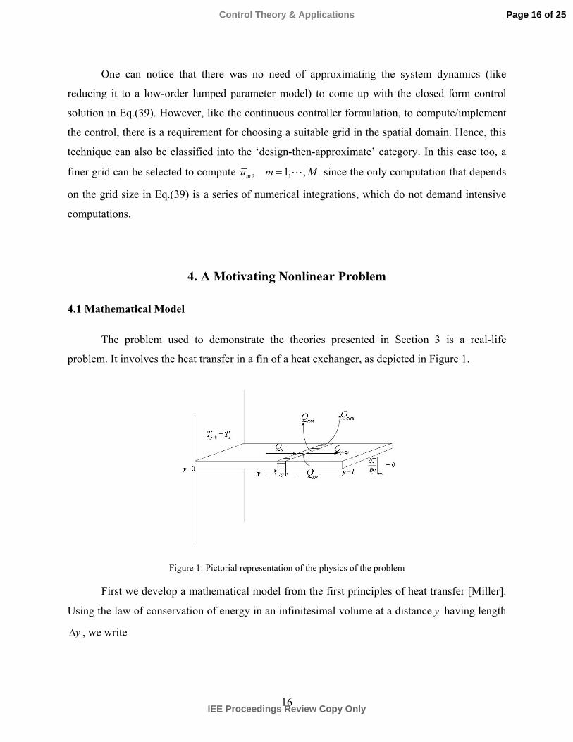
problem. It involves the heat transfer in a fin of a heat exchanger, as depicted in Figure 1.

Figure 1: Pictorial representation of the physics of the problem

First we develop a mathematical model from the first principles of heat transfer [Miller].

Using the law of conservation of energy in an infinitesimal volume at a distance y having length

y∆ , we write

Page 16 of 25



17

y gen y y conv rad chgQ Q Q Q Q Q+∆+ = + + + (40)

where yQ is the rate of heat conducted in, genQ is the rate of heat generated, y yQ +∆ is the rate of

heat conducted out, convQ is the rate of heat convected out, radQ is the rate of heat radiated out and

chgQ is the rate of heat change. Next, from the laws of physics for heat transfer [Miller], we can

write the following expressions

y

TQ kAy

∂= − ∂

(41a)

genQ S A y= ∆ (41b)

( )1convQ h P y T T∞= ∆ − (41c)

( )2

4 4radQ P y T Tε σ ∞= ∆ − (41d)

chg

TQ C A yt

ρ ∂ = ∆ ∂ (41e)

In Eqs.(41a-e), ( ),T t y represents the temperature (this is the state ( ),x t y in the context

of discussion in Section 3), which is a function of both time t and spatial location y . ( ),S t y is

the rate of heat generation per unit volume (this is the control u in the context of discussion in

Section 3) for this problem. The meanings of various parameters and their numerical values used

and are given in Table 1.

Table 1: Definitions and numerical values of the parameters

Parameter Meaning Numerical value

k Thermal conductivity ( )180 / oW m C

A Cross sectional area 22 cm

P Perimeter 9 cm

h Convective heat transfer coefficient ( )2 05 /W m C

1T∞ Temperature of the medium in the

immediate surrounding of the surface 30 C°

Page 17 of 25



18

2T∞ Temperature at a far away place in the

direction normal to the surface 40 C− °

ε Emissivity of the material 0.2

σ Stefan-Boltzmann constant 8 2 45.669 10 /W m K−×

ρ Density of the material 32700 /kg m

C Specific heat of the material ( )860 /J kg C°

The values representing of the properties of the material were chosen assuming

Aluminum. The area A and perimeter P have been computed assuming the a fin of dimension

40 4 0.5cm cm cm× × . Note that we have made a one-dimensional approximation for the

dynamics, assuming uniform temperature in the other two dimensions being arrived at

instantaneously.

Using Taylor series expansion and considering a small 0y∆ → , we can write

yy y y

QQ Q y

y+∆

∂ ≈ + ∆ ∂

(42)

Using Eqs.(41a-e) and (42) in Eq.(40) and simplifying, we can write

( ) ( )1 2

24 4

2

1T k T P h T T T T St C y A C C

ε σρ ρ ρ∞ ∞

∂ ∂ = − − + − + ∂ ∂ (43)

For convenience, we define ( )1 /k Cα ρ , ( ) ( )2 /Ph A Cα ρ− , ( ) ( )3 /P A Cα εσ ρ− and

( )1/ Cβ ρ , we can rewrite Eq.(43) as

( ) ( )1 2

24 4

1 2 32

T T T T T T St y

α α α β∞ ∞

∂ ∂= + − + − + ∂ ∂

(44)

Along with Eq.(44), we consider the following boundary conditions

0 , 0y w

y L

TT Ty=

=

∂= =

∂ (45)

Page 18 of 25



19

where wT is the wall temperature. We have assumed insulated boundary condition at the tip with

the assumption that either there is some physical insulation at the tip or the heat loss at the tip

due to convection and radiation is negligible (mainly because of its low surface area). The goal

for the controller was to make sure that the actual temperature profile ( ) ( )*,T t y T y→ , where

we chose ( )*T y to be a constant (with respect to time) temperature profile. ( )*T y was

generated by using the following expression

( ) ( )* y

w w tipT y T T Tζ−

= + − (46)

In Eq.(46) we chose the wall temperature 0150wT C= , fin tip temperature 0130tipT C= and the

decaying parameter 20ζ = . The selection such a ( )*T y from Eq.(46) was motivated by the fact

that it leads to a smooth continuous temperature profile across the spatial dimension y . This

selection of ( )*T y satisfies the boundary condition at 0y = exactly and at y L=

approximately, with a very small (rather negligible) approximation error. Note that the system

dynamics is in control-affine form and ( ), , , 0g x x x β′ ′′ = ≠ . Moreover, there is no boundary

control action. This is compatible with the class of DPS for which we have developed the control

synthesis theories in Section 3.

In the discrete controller case, the system dynamics in Eq.(44) will get modified to

( ) ( )1 2

24 4

1 2 321

M

mm

T T T T T T St y

α α α β∞ ∞=

∂ ∂= + − + − + ∂ ∂

∑ (47)

However, the boundary conditions remain same as in Eq.(45).

4.2 Synthesis of Continuous Controller

In our simulation studies with the continuous controller formulation, we selected the

control gain as 1/k τ= , where 30 secτ = . We assumed ( )r y as a constant c +∈ , and hence,

were able to use the simplified formula for the control in Eq.(17). Hence a numerical value for

( )r y was not necessary for the simulation studies.

Page 19 of 25



20

First we chose an initial condition (profile) for the temperature as obtained from the

expression ( ) ( )0, 0,mT y T x y= + , where 0150mT C= (a constant value) serves as the mean

temperature and ( )0,x y represents the deviation from mT . Taking 50A = we computed ( )0,x y

as ( ) ( ) ( ) ( )0, / 2 / 2 cos 2 /x y A A y Lπ π= + − + . Applying the controller as synthesized in

Eq.(22), we simulated the system in Eqs.(44)-(45) from time 0 0t t= = to 5minft t= = . The

results obtained are as in Figure 2(a,b). We can see from Figure 2(a) that the goal of tracking

( )*T y is met without any problem. The associated control (rate of energy input) profile ( ),S t y

obtained is as shown in Figure 2(b). It is important to note that even as ( ) ( )*,T t y T y→ , there

is no control singularity. In fact the control profile develops (converges) towards the steady-state

control profile (see Eq.(19)).

Figure 2(a): Evolution of the temperature (state)

profile from a sinusoidal initial condition

Figure 2(b): Rate of energy input (control) for the

evolution of temperature profile in Figure 2(a)

Next, to demonstrate that similar results will be obtained for any arbitrary initial

condition of the temperature profile ( )0,T y , we considered a number of random profiles for

( )0,T y and carried out the simulation studies. The random profiles using the relationship

( ) ( )0, 0,mT y T x y= + , where ( )0,x y was generated using the concept of Fourier Series, such

that it satisfies ( ) 2 2

1 max0,x y k x≤ , ( ) 2 2

2 max0,x y k x′ ′≤ and ( ) 2 2

3 max0,x y k x′′ ′′≤ . The values for

maxx ,

maxx′ and

maxx′′ were computed using an envelope profile ( ) ( )sin /envx y A y Lπ= . The

Page 20 of 25



21

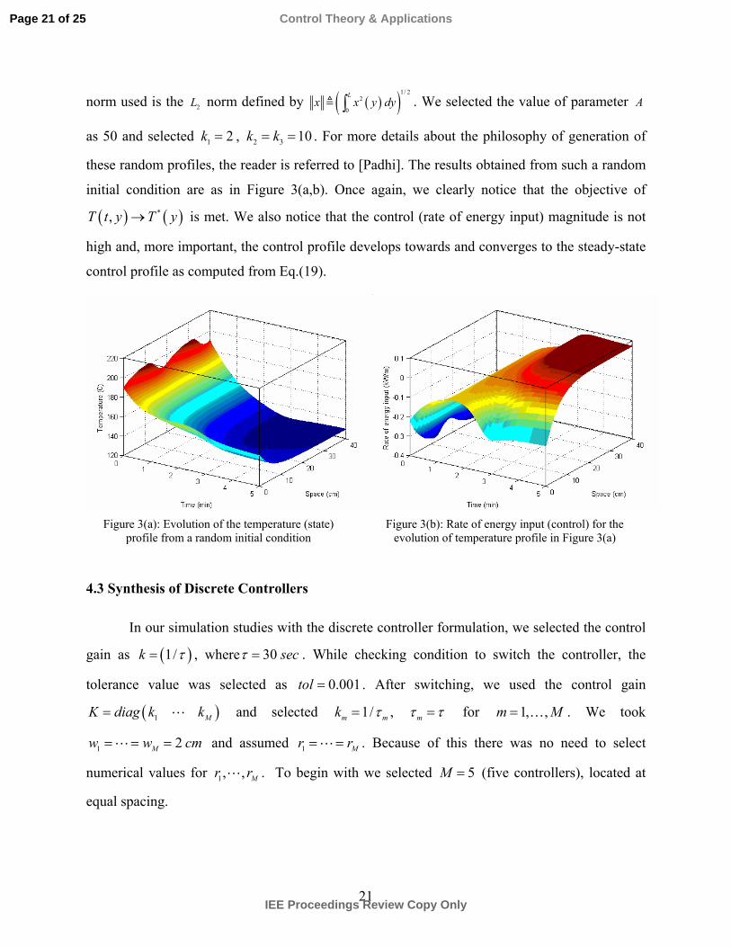
norm used is the 2L norm defined by ( )( )1/ 22

0

Lx x y dy∫ . We selected the value of parameter A

as 50 and selected 1 2k = , 2 3 10k k= = . For more details about the philosophy of generation of

these random profiles, the reader is referred to [Padhi]. The results obtained from such a random

initial condition are as in Figure 3(a,b). Once again, we clearly notice that the objective of

( ) ( )*,T t y T y→ is met. We also notice that the control (rate of energy input) magnitude is not

high and, more important, the control profile develops towards and converges to the steady-state

control profile as computed from Eq.(19).


profile from a random initial condition

Figure 3(b): Rate of energy input (control) for the


4.3 Synthesis of Discrete Controllers

In our simulation studies with the discrete controller formulation, we selected the control

gain as ( )1/k τ= , where 30 secτ = . While checking condition to switch the controller, the

tolerance value was selected as 0.001tol = . After switching, we used the control gain

( )1 MK diag k k= and selected 1/m mk τ= , mτ τ= for 1, ,m M= … . We took

1 2Mw w cm= = = and assumed 1 Mr r= = . Because of this there was no need to select

numerical values for 1, , Mr r . To begin with we selected 5M = (five controllers), located at

equal spacing.

Page 21 of 25



22

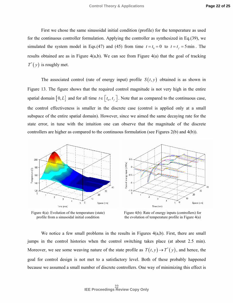
First we chose the same sinusoidal initial condition (profile) for the temperature as used

for the continuous controller formulation. Applying the controller as synthesized in Eq.(39), we

simulated the system model in Eqs.(47) and (45) from time 0 0t t= = to 5minft t= = . The

results obtained are as in Figure 4(a,b). We can see from Figure 4(a) that the goal of tracking

( )*T y is roughly met.

The associated control (rate of energy input) profile ( ),S t y obtained is as shown in

Figure 13. The figure shows that the required control magnitude is not very high in the entire

spatial domain [ ]0, L and for all time 0 , ft t t ∈ . Note that as compared to the continuous case,

the control effectiveness is smaller in the discrete case (control is applied only at a small

subspace of the entire spatial domain). However, since we aimed the same decaying rate for the

state error, in tune with the intuition one can observe that the magnitude of the discrete

controllers are higher as compared to the continuous formulation (see Figures 2(b) and 4(b)).



Figure 4(b): Rate of energy inputs (controllers) for the evolution of temperature profile in Figure 4(a)

We notice a few small problems in the results in Figures 4(a,b). First, there are small

jumps in the control histories when the control switching takes place (at about 2.5 min).

Moreover, we see some weaving nature of the state profile as ( ) ( )*,T t y T y→ , and hence, the

goal for control design is not met to a satisfactory level. Both of these probably happened

because we assumed a small number of discrete controllers. One way of minimizing this effect is

Page 22 of 25



23

to increase the number of controllers. Next, we selected ten controllers (instead of five) and

carried out the simulation again. The results are shown in Figure 5(a,b). It is quite clear from this

figure that the weaving nature is substantially smaller and the goal ( ) ( ) [ ]*, , 0,T t y T y y L→ ∀ ∈

is met with more accuracy. Also note that as compared to the case with five controllers, here the

control effectiveness is higher and subsequently the magnitudes of the controllers are smaller

(compare Figures 4(b) and 5(b)).



Figure 5(b): Rate of energy inputs (controllers) for the


To demonstrate that similar results will be obtained for any arbitrary initial condition of

the temperature profile ( )0,T y , next we considered a number of random profiles for ( )0,T y

(generated the same way as in Section 4.2) and carried out the simulation studies. The results

obtained from such a random initial condition are quite satisfactory in the sense that the tracking

objective was met. To contain the length of the paper, however, we do not include those results.

5. Conclusions

Based on the newly proposed optimal dynamic inversion theory, two stabilizing state

feedback control design approaches are presented for a class of nonlinear distributed parameter

systems. One approach combines the dynamic inversion with variational optimization, whereas

Page 23 of 25



24

the other one (which is more relevant in practice) can be applied when there are a number of

discrete actuators located at distinct places in the spatial domain. These new techniques can be

classified as “design-then-approximate” methods, which are in general more elegant than the

“approximate-then-design” methods. The formulation leads to a closed form control solution,

and hence, is not computationally intensive. To demonstrate the potential of the proposed

techniques, a real-life temperature control problem for a heat transfer application is solved, first

assuming a continuous actuator and then assuming a set of discrete actuators and promising

numerical results are obtained.

References

1. Annaswamy A., Choi J. J., Sahoo D., Active Closed Loop Control of Supersonic Impinging Jet Flows

Using POD Models, Proceedings of the 41st IEEE Conference on Decision and Control, Las Vegas,

2002.

2. Arian E., Fahl M. and Sachs E. W., Trust-region Proper Orthogonal Decomposition for Flow Control,

NASA/CR-2000-210124, ICASE Report No. 2000-25.

3. Bameih B., The Structure of Optimal Controllers of Spatially-invariant Distributed Parameter

Systems. Proceedings of the Conference on Decision & Control, 1997, 1056-1061.

4. Banks H. T., Rosario R. C. H and Smith R. C., Reduced-Order Model Feedback Control Design:

Numerical Implementation in a Thin Shell Model, IEEE Transactions on Automatic Control, Vol. 45,

2000, 1312-1324.

5. Bryson A. E. and Ho Y. C., Applied Optimal Control, London: Taylor and Francis, 1975.

6. aBurns J.A. and King, B.B., Optimal sensor location for robust control of distributed parameter

systems. Proceedings of the Conference on Decision and Control, 1994, 3967- 3972.

7. bBurns J. and King B. B., A Reduced Basis Approach to the Design of Low-order Feedback

Controllers for Nonlinear Continuous Systems, Journal of Vibration and Control, Vol.4, 1998, 297-

323.

8. Christofides P. D., Nonlinear and Robust Control of PDE Systems – Methods and Applications to

Transport-Reaction Processes, Birkhauser , Boston, 2000.

Page 24 of 25



25

9. Curtain R. F. and Zwart H. J., An Introduction to Infinite Dimensional Linear Systems Theory,

Springer-Verlag, New York, 1995.

10. Enns, D., Bugajski, D., Hendrick, R. and Stein, G., Dynamic Inversion: An Evolving Methodology

for Flight Control Design, International Journal of Control, Vol.59, No.1,1994, pp.71-91.

11. Holmes P., Lumley J. L. and Berkooz G., Turbulence, Coherent Structures, Dynamical Systems and

Symmetry, Cambridge University Press, 1996, 87-154.

12. Kim, B. S. and Calise, A. J., “Nonlinear Filight Control using Neural Networks”, AIAA Journal of

Guidance, Control, and Dynamics, Vol. 20, No. 1, 1997, pp.26-33.

13. Lasiecka I., Control of Systems Governed by Partial Differential Equations: A Historical Perspective,

Proceedings of the 34th Conference on Decision and control, 1995, 2792-2796.

14. Lane, S. H. and Stengel, R. F., Flight Control Using Non-Linear Inverse Dynamics, Automatica,

Vol.24, No.4, 1988, pp.471-483.

15. McFarland, M. B., Rysdyk, R. T., and Calise A. J., “Robust Adaptive Control Using Single-Hidden-

layer Feed-forward Neural Networks,” Proceeding of the American Control Conference, 1999, pp.

4178-4182.

16. Miller A. F., Basic Heat and Mass Transfer, Richard D. Irwin Inc., MA, 1995.

17. Ngo, A. D., Reigelsperger, W. C. and Banda, S. S., Multivariable Control Law Design for A Tailless

Airplanes, Proceedings of the AIAA Conference on Guidance, Navigation and Control, 1996, AIAA-

96-3866.

18. Padhi R. and Balakrishnan S. N., Proper Orthogonal Decomposition Based Optimal Neurocontrol

Synthesis of a Chemical Reactor Process Using Approximate Dynamic Programming, Neural

Networks, Vol. 16, 2003, pp. 719-728.

19. Ravindran S. S., Adaptive Reduced-Order Controllers for a Thermal Flow System Using Proper

Orthogonal Decomposition, SIAM Journal on Scientific Computing, Vol.23, No.6, 2002, pp.1924-

1942.

20. Slotine, J-J. E. and Li, W., Applied Nonlinear Control, Prentice Hall, 1991.

Page 25 of 25



iee proceedings review copy only - missouri university …web.mst.edu/~autosys/papers/008.pdfoptimal...

Documents