IEEE 802.11 Wi-Fi Access Point DensityEstimation with Capture-Recapture Models

Andreas Achtzehn, Ljiljana Simic, Marina Petrova and Petri MahonenInstitute for Networked Systems

RWTH Aachen UniversityKackertstrasse 9, D-52072 Aachen, Germany

Email: {aac,lsi,mpe,pma}@inets.rwth-aachen.de

Abstract—The estimation of IEEE 802.11 Wi-Fi access point(AP) densities is an important cornerstone in deriving accuratemodels for the deployment structure of opportunistic wirelessnetworks. Such densities are usually derived through large-scalewardriving-like measurement campaigns with COTS devices. Dueto shielding, limited receiver sensitivity, and sampling densityconstraints, in general only a subset of Wi-Fi APs can beobserved. Furthermore, repeated measurement campaigns showthat even if an AP has been observed in one visit to a study area,it may not be observed in subsequent visits, due to small-scaledeviations in the measurement locations and unavoidable changesin the radio environment such as moving vehicles and pedestrians.This motivates our study of the application of capture-recapturemodels to establish more accurate estimates of the actual numberof APs in a study area. We approach this problem by firstdeveloping a general system model and mathematical frame-work for AP observability. As we assume temporally constantpopulation sizes but potential inhomogeneities in observationprobabilities, we then assess the performance of two applicablepopulation density estimators, namely the Lincoln-Petersen andjackknife estimators, through a simulation study. We demonstratethe practical significance of the proposed capture-recapturemethodology by applying it to a data set from an extensiveurban Wi-Fi measurement campaign that we have carried outin Cologne, Germany, quantifying the achievable gains and theestimators’ sensitivity to the measurement campaign design. Weshow that applying the capture-recapture techniques providesthe practical advantage of yielding a similar accuracy in theestimation of Wi-Fi density even with significantly fewer measure-ment locations than surveyed in the full campaign. However, ourresults indicate that a high receiver sensitivity remains essentialfor such wardriving-like measurements, i.e. less sophisticatedmeasurement setups such as smartphones will introduce higherrors in the AP density estimation.

I. INTRODUCTION

An essential step in the evolution towards future wirelessnetworks is the densification of the access network. In or-der to meet increased capacity demands, smaller and moredensely distributed cells will be needed to bring the networkcloser to the terminal [1]. The development of algorithms, thequantification of achievable data rates, and the assessment ofthe prospects of such deployments will necessarily rely onaccurate models for the location and number of infrastructurecomponents in typical usage scenarios.

Current installations of Wi-Fi access points (APs) maybe considered a good real-world example indicative of thestructure of future opportunistic wireless networks, because

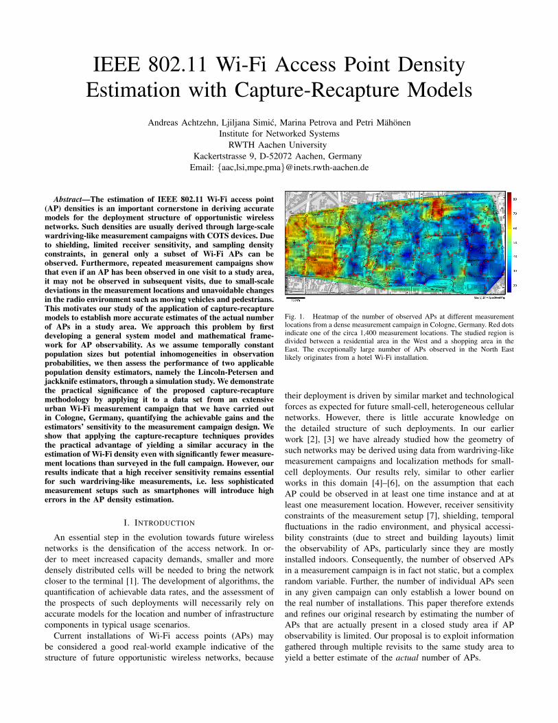
Fig. 1. Heatmap of the number of observed APs at different measurementlocations from a dense measurement campaign in Cologne, Germany. Red dotsindicate one of the circa 1,400 measurement locations. The studied region isdivided between a residential area in the West and a shopping area in theEast. The exceptionally large number of APs observed in the North Eastlikely originates from a hotel Wi-Fi installation.

their deployment is driven by similar market and technologicalforces as expected for future small-cell, heterogeneous cellularnetworks. However, there is little accurate knowledge onthe detailed structure of such deployments. In our earlierwork [2], [3] we have already studied how the geometry ofsuch networks may be derived using data from wardriving-likemeasurement campaigns and localization methods for small-cell deployments. Our results rely, similar to other earlierworks in this domain [4]–[6], on the assumption that eachAP could be observed in at least one time instance and at atleast one measurement location. However, receiver sensitivityconstraints of the measurement setup [7], shielding, temporalfluctuations in the radio environment, and physical accessi-bility constraints (due to street and building layouts) limitthe observability of APs, particularly since they are mostlyinstalled indoors. Consequently, the number of observed APsin a measurement campaign is in fact not static, but a complexrandom variable. Further, the number of individual APs seenin any given campaign can only establish a lower bound onthe real number of installations. This paper therefore extendsand refines our original research by estimating the number ofAPs that are actually present in a closed study area if APobservability is limited. Our proposal is to exploit informationgathered through multiple revisits to the same study area toyield a better estimate of the actual number of APs.

In this paper we go beyond simple counting of the indi-vidual APs by applying methods and mathematical tools thathave originally been developed for application to biology.Namely, we observe that the counting of individual APsin wardriving-like measurement campaigns is similar to thecommon problem in biology of estimating wildlife populationsizes [8]. Propagation and shielding effects result in APsbeing only occasionally observable, and thus the visibility ofindividual APs changes between visits to the same surveyarea, i.e. there is an AP-dependent observation probability.Various mathematical tools for deriving total population sizesfrom multiple visits to the same study area have been devel-oped in biology, which require capturing, tagging, releasing,and recapturing animals on different occasions; due to thismethodology, they are often referred to as capture-recapturemodels. They have also been recently transferred to otherscientific fields, e.g. in the estimation of programming errorsin large software projects [9]. In this paper, we introduce thepopular Lincoln-Petersen and jackknife estimators, and applythem to the problem of estimating Wi-Fi AP densities frommeasurement data. We have initially selected these estimatorsas they are tailored to scenarios with constant populationsizes (which can be safely assumed over the time scale of aWi-Fi measurement campaign) and potential inhomogeneitiesof observations probabilities (due to AP placement and localenvironment variability). In addition to testing the estimatorsagainst synthetic data from a proposed system model for APobservability, we also present our results from a large-scalemeasurement campaign we have carried out in the city centreof Cologne, Germany. We find that the proposed predictorsenable a thinning of the measurement locations set, i.e. theyallow a reduction of the surveying effort with reasonable lossin prediction accuracy. However, a high receiver sensitivityremains essential for the accurate estimation of total APcounts. The application of capture-recapture methods is thusbeneficial for deriving robust models of the spatial structureof opportunistic wireless networks, since accurate estimates ofnode density are highly relevant for analyses on interference,coverage, and connectivity.

This paper is organized as follows. In Section II we discussthe constraints on AP observability in a realistic measurementcampaign and derive a mathematical model for the observationprobability based on extreme value theory. In Section III weintroduce capture-recapture models as a means of estimatingthe number of APs in a study area. In Section IV we applythese models to a simulated scenario with a known numberof APs and limited observability. In Section V we analyze theperformance of the estimators for the Cologne data set. Thepaper is concluded in Section VI.

II. OBSERVABILITY OF WI-FI APS

The basis of our empirical study is data from a measurementcampaign that we carried out in mid-2013 in the urban centreof the metropolitan city of Cologne, Germany. Using a custombicycle setup [3] with an antenna mast and three COTS Wi-Fiadapters that connect into a laptop, we scanned for Wi-Fi APs

−110 −100 −90 −80 −70 −60 −50 −40 −30 −20 −100

0.01

0.02

0.03

0.04

0.05

0.06

0.07

0.08

0.09

Maximum AP signal strength [dBm]

pdf

Signal strength valuesunmodified fiterror−adjusted fit

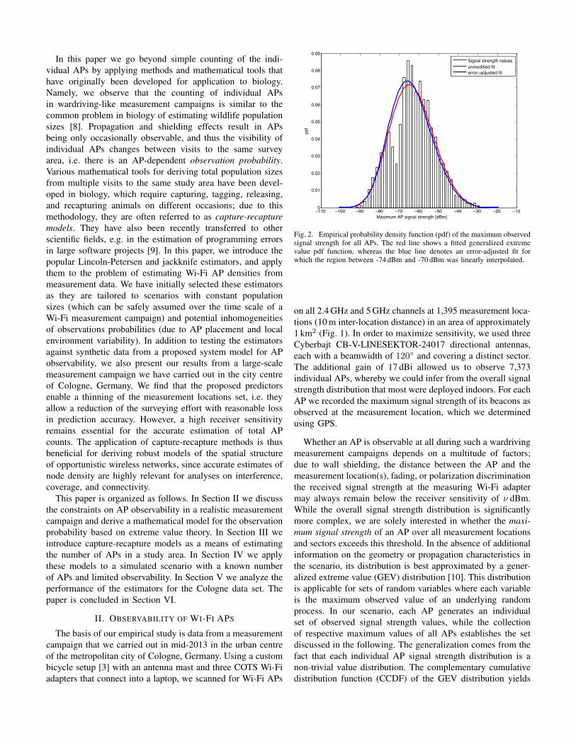
Fig. 2. Empirical probability density function (pdf) of the maximum observedsignal strength for all APs. The red line shows a fitted generalized extremevalue pdf function, whereas the blue line denotes an error-adjusted fit forwhich the region between -74 dBm and -70 dBm was linearly interpolated.

on all 2.4 GHz and 5 GHz channels at 1,395 measurement loca-tions (10 m inter-location distance) in an area of approximately1 km2 (Fig. 1). In order to maximize sensitivity, we used threeCyberbajt CB-V-LINESEKTOR-24017 directional antennas,each with a beamwidth of 120◦ and covering a distinct sector.The additional gain of 17 dBi allowed us to observe 7,373individual APs, whereby we could infer from the overall signalstrength distribution that most were deployed indoors. For eachAP we recorded the maximum signal strength of its beacons asobserved at the measurement location, which we determinedusing GPS.

Whether an AP is observable at all during such a wardrivingmeasurement campaigns depends on a multitude of factors;due to wall shielding, the distance between the AP and themeasurement location(s), fading, or polarization discriminationthe received signal strength at the measuring Wi-Fi adaptermay always remain below the receiver sensitivity of ν dBm.While the overall signal strength distribution is significantlymore complex, we are solely interested in whether the maxi-mum signal strength of an AP over all measurement locationsand sectors exceeds this threshold. In the absence of additionalinformation on the geometry or propagation characteristics inthe scenario, its distribution is best approximated by a gener-alized extreme value (GEV) distribution [10]. This distributionis applicable for sets of random variables where each variableis the maximum observed value of an underlying randomprocess. In our scenario, each AP generates an individualset of observed signal strength values, while the collectionof respective maximum values of all APs establishes the setdiscussed in the following. The generalization comes from thefact that each individual AP signal strength distribution is anon-trivial value distribution. The complementary cumulativedistribution function (CCDF) of the GEV distribution yields

an estimate for the probability of an AP being observed, i.e.

Pr{AP observed} = 1− exp

{−[1 + ξ

ν − µσ

]−1/ξ}, (1)

where µ, σ, and ξ are the scenario and measurement setup-specific location, scale, and shape parameter of the distribu-tion, respectively.

Fig. 2 shows the results of fitting our theoretical model ofAP observation probabilities in (1) to the measurement datafrom our Cologne campaign. We have excluded data fromthose APs that were only observed within 50 m to the border ofour study area in order to minimize edge effects. We found thatthe employed Wi-Fi adapters reported significantly more eventhan odd signal strength values, which leads us to concludethat the reporting accuracy for the particular COTS devices islimited to 2 dB steps. For postprocessing we therefore roundedthe signal strength values to the closest even power value. Thehistogram plot of Fig. 2 furthermore exhibits an unexpectedlylow relative number of samples at the range between -74 dBmand -70 dBm. Assuming this to be an unstable operation stateof the Wi-Fi adapter, we have instead linearly interpolated thesample density to yield an error-adjusted fit.

However, despite these postprocessing steps, the numericalvalues of the fitting process do not significantly differ. ξ isestimated as -0.2, i.e. the empirical distribution resembles areverse Weibull (type III) distribution. This is an interesting re-sult as it indicates that the distribution is more strongly affectedby the upper bound of the observed signal strength values thanby the lower bound of the receiver sensitivity. The mode of theprobability density function is at -66 dBm, which is close to theestimated location parameter value of µ = −68 dBm, wherebythe scale is approximately σ = 10 dB. We note that the shapeof the distribution also matches intuition. While, in principle,there is a nearly infinite number of APs at larger distances thatcontribute to the lower tail of the distribution (although notbeing observable), the maximum transmit power of each APis constrained by regulations. Thus, in a wardriving campaignit is impossible to observe APs beyond the maximum transmitpower, i.e. the distribution is necessarily upper bounded.

III. APPLYING CAPTURE-RECAPTURE MODELS

Differences in propagation and slight variations in measure-ment locations will result in deviations in the sets of observedAPs between different visits to the same study area. This isbecause the received signal strength of an APs will eventuallyremain below the receiver sensitivity, and thus render an APoccasionally unobservable. The fundamental idea of capture-recapture models is thus to derive the probability of observingan AP and use this metric for estimating the overall populationsize. If measurement locations are sufficiently close, multiplevisits to the surveyed area thereby may also be emulatedby splitting the measurement locations into non-overlappingsets. This is the technique we apply in our empirical study inSection V.

A basic assumption of simple capture-recapture models isthat the probability of observing an AP over multiple revisits

to the surveyed area is homogeneous over the population,i.e. that the probability of observing an AP is the samefor all APs. Assuming that the same effort, i.e. the samenumber, location distribution, and duration of measurements,is used by the experimenter in the initial capturing process andany recapturing round, the ratio of initially captured devicescompared to the estimated total number of devices NLP isequivalent to the ratio of the devices captured both times tothe overall number of devices captured in the second round ofthe capturing. This so-called Lincoln-Petersen estimator [8] isthe first population size predictor we consider; it is defined as

n2

NLP=M

n1⇔ NLP =

n1 × n2M

, (2)

where n1 is the number of APs initially identified, n2 isnumber of APs found in the recapture, and M is the totalnumber of distinct APs found.

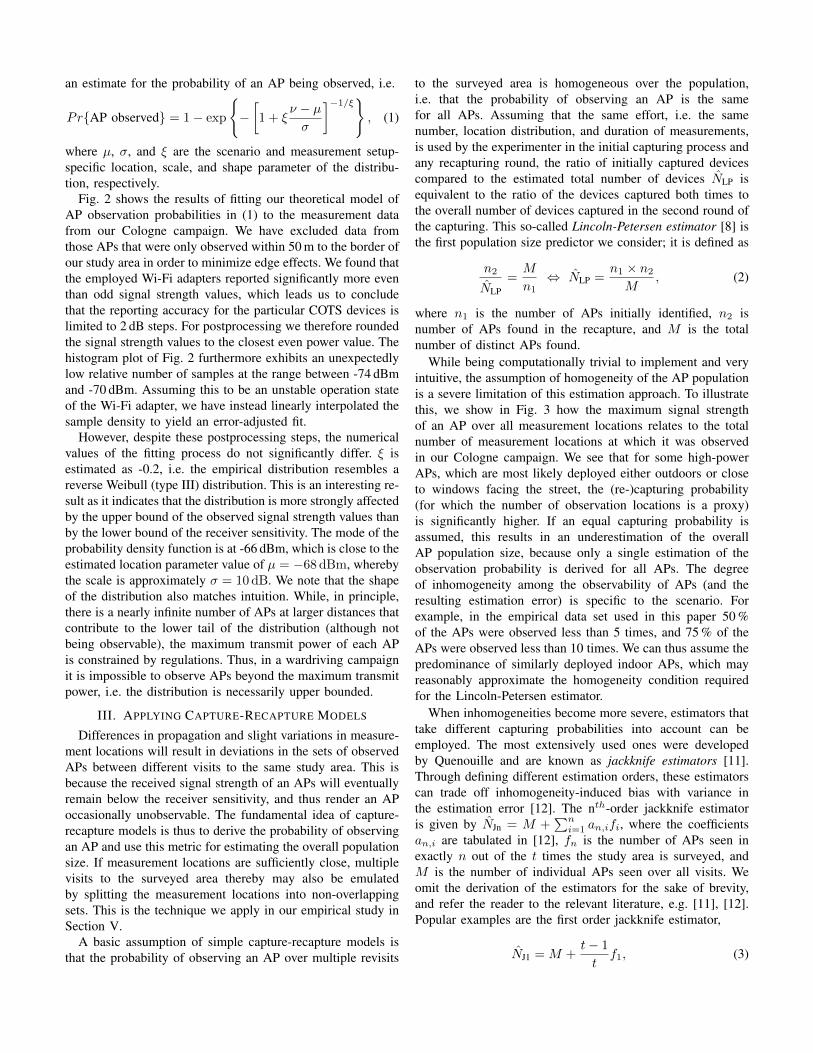
While being computationally trivial to implement and veryintuitive, the assumption of homogeneity of the AP populationis a severe limitation of this estimation approach. To illustratethis, we show in Fig. 3 how the maximum signal strengthof an AP over all measurement locations relates to the totalnumber of measurement locations at which it was observedin our Cologne campaign. We see that for some high-powerAPs, which are most likely deployed either outdoors or closeto windows facing the street, the (re-)capturing probability(for which the number of observation locations is a proxy)is significantly higher. If an equal capturing probability isassumed, this results in an underestimation of the overallAP population size, because only a single estimation of theobservation probability is derived for all APs. The degreeof inhomogeneity among the observability of APs (and theresulting estimation error) is specific to the scenario. Forexample, in the empirical data set used in this paper 50 %of the APs were observed less than 5 times, and 75 % of theAPs were observed less than 10 times. We can thus assume thepredominance of similarly deployed indoor APs, which mayreasonably approximate the homogeneity condition requiredfor the Lincoln-Petersen estimator.

When inhomogeneities become more severe, estimators thattake different capturing probabilities into account can beemployed. The most extensively used ones were developedby Quenouille and are known as jackknife estimators [11].Through defining different estimation orders, these estimatorscan trade off inhomogeneity-induced bias with variance inthe estimation error [12]. The nth-order jackknife estimatoris given by NJn = M +

∑ni=1 an,ifi, where the coefficients

an,i are tabulated in [12], fn is the number of APs seen inexactly n out of the t times the study area is surveyed, andM is the number of individual APs seen over all visits. Weomit the derivation of the estimators for the sake of brevity,and refer the reader to the relevant literature, e.g. [11], [12].Popular examples are the first order jackknife estimator,

NJ1 = M +t− 1

tf1, (3)

0

10

20

30

40

50

60

70

80

�

�

�

�

�

�

�

�

�

�

�

�

�

�

�

�

�

�

�

�

�

�

�

�

�

�

�

�

�

�

�

�

�

�

�

Maximum signal strength observed [dBm]

Num

ber o

f obs

erva

tions

Fig. 3. Maximum signal strength of observation vs. the number of measure-ment locations at which an AP was observed during Cologne measurementcampaign.

the second order jackknife estimator,

NJ2 = M +2t− 3

tf1 −

(t− 2)2

t(t− 1)f2, (4)

and the third order jackknife estimator,

NJ3 = M +3t− 6

tf1 − . . .

3t2 − 15t+ 19

t(t− 1)f2 +

(t− 3)3

t(t− 1)(t− 2)f3. (5)

IV. SIMULATION RESULTS

In order to evaluate the prediction accuracy of the differentestimators introduced in Section III in the context of Wi-FiAP density estimation, we have simulated signal strength dis-tributions for a known population size of N = 1,000 APs. Themaximum signal strength Pmax,j of each AP j is modelled bythe empirical distribution function in Fig. 2. For each iterationi of the capturing process, we add a zero-mean Gaussianshadowing term Ξi,j to Pmax,j . This term models attenuationwhich may originate from obstacles and small-scale offsets inthe propagation path. Our empirical data set shows that thestandard deviation of this term is approximately σs = 5.5 dB,thus we selected this value also for our simulation1. An AP isconsidered “observed” in iteration i iff Pmax,j + Ξi,j ≥ ν. Wehave repeated the simulation 100,000 times to acquire meanvalues and distributions of the different predictors.

The expected number of individual APs observed for adifferent number of iterations t can be determined analyticallyin this model as

1We note that our model thereby implicitly assumes correlated shadowing,because locations of maximum observed signal strength for each individualiteration of the survey are usually close to each other.

500 600 700 800 900 10000

0.005

0.01

0.015

0.02

0.025

0.03

0.035

Estimated number of APs

pdf

Lincoln−Petersen1st order jackknife (t = 2)1st order jackknife (t = 3)2nd order jackknife (t = 3)1st order jackknife (t = 4)2nd order jackknife (t = 4)

mea

n #A

Ps o

bser

ved

(t =

2)

mea

n #A

Ps o

bser

ved

(t =

3)

mea

n #A

Ps o

bser

ved

(t =

4)

(a) ν = -70 dBm

500 600 700 800 900 10000

0.005

0.01

0.015

0.02

0.025

0.03

0.035

Estimated number of APs

pdf

Lincoln−Petersen1st order jackknife (t = 2)1st order jackknife (t = 3)2nd order jackknife (t = 3)1st order jackknife (t = 4)2nd order jackknife (t = 4)

mea

n #A

Ps o

bser

ved

(t =

2)

mea

n #A

Ps o

bser

ved

(t =

3)

mea

n #A

Ps o

bser

ved

(t =

4)

(b) ν = -60 dBm

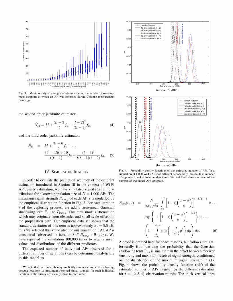
Fig. 4. Probability density functions of the estimated number of APs for asimulation of 1,000 Wi-Fi APs for different decodability thresholds ν, numberof captures t, and estimation algorithms. Vertical lines show the mean of thenumber of individual APs observed.

Nobs(t, ν) =N

σσs√

2π

∞∫−∞

[1 + ξ

(x− µσ

)](−1/ξ)−1× . . .

exp

{−1

[1 + ξ

(x− µσ

)]−1/ξ}× . . .1−

ν−x∫−∞

exp

{− t

2σ2s

y2}dy

dx. (6)

A proof is omitted here for space reasons, but follows straight-forwardly from deriving the probability that the Gaussianshadowing term Ξi,j is smaller than the offset between receiversensitivity and maximum received signal strength, conditionedon the distribution of the maximum signal strength in (1).Fig. 4 shows the probability density function (pdf) of theestimated number of APs as given by the different estimatorsfor t = {2, 3, 4} observation rounds. The thick vertical lines

indicate the mean number of APs observed for a given t, asgiven by (6), cf. the real population size of 1,000 APs. For areceiver sensitivity of ν = −70 dBm, Fig.4a shows that theLincoln-Petersen estimator yields the largest overall estimationerror with a mean value that is 21 % smaller than the actualnumber of APs. The first order jackknife estimator for thesame number of iterations, t = 2, performs slightly better withan estimation error of only 18.5 % on average. Additionally,the jackknife estimation exhibits a smaller error spread, as isapparent from the higher value of the mode. When the numberof iterations is increased, the jackknife estimators convergetowards the actual number of APs in the simulation. The maindifference here lies in the variance. The second order estimatorpredicts a wider range of values relative to its mean comparedto the first order jackknife. However, even with this extendedspread the average error remains smaller than for the first orderestimator. We have conducted further experiments also withhigher order jackknife estimators not shown here, however,we found no additional gains. Furthermore, in order for theseestimators to be applicable, the number of iterations t must belarger than the the order n minus 1, which may be a practicalconstraint in a measurement campaign.

Comparing Fig. 4a and Fig. 4b shows that when the decob-ability threshold is raised, which may model a case when ameasurement campaign is carried out using less sophisticated(i.e. higher receiver sensitivity) equipment, the number ofobserved APs further decreases. Here, the real benefit ofadditional visits to the study area comes into play, as we cansee for the case of t = 4 iterations. The second order jackknifeestimator yields an average error of only 27 % compared tothe loss in observed APs of 41 %. However, the estimationspread becomes significantly larger, ranging between 630 and802 APs.

V. EMPIRICAL RESULTS

In this section we apply the capture-recapture estimatorsintroduced in Section III to the data set from our extensiveWi-Fi measurement campaign described in Section II. We notethat, since the real number of APs within the surveyed areais by definition unknown, we cannot argue about the absoluteaccuracy of the AP population size estimate. Instead, in thissection we study the effect on the estimators’ performancewhen the sampling accuracy or effort are artificially decreasedby thinning of the data set. The results we present here therebygive important insights into the requirements for real-worldWi-Fi measurement campaigns, and demonstrate the benefitsof applying capture-recapture models to improve AP densityestimation.

The practical application of these models requires multiplevisits to the study area. However, if the measurement locationdensity is high, a reasonable technique for emulating multiplevisits is to split the measurement locations into t equal-sizedand disjoint sets. Splitting needs to be done in a manner so asto minimize inter-set distances, i.e. neighbouring measurementlocations should ideally be in different sets. We found that forup to four sets the sampling density of our data set suffices so

−90 −85 −80 −75 −70 −65 −60 −55 −50 −45 −400

1000

2000

3000

4000

5000

6000

7000

8000

9000

Decodability threshold [dBm]

Estim

ated

num

ber o

f APs

Lincoln−Petersen1st order jackknife (t = 2)1st order jackknife (t = 3)2nd order jackknife (t = 3)1st order jackknife (t = 4)2nd order jackknife (t = 4)3rd order jackknife (t = 4)Reference: Observed number of APs

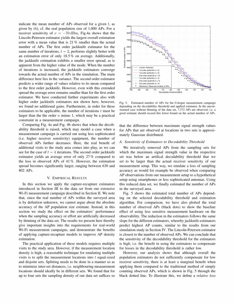
Fig. 5. Estimated number of APs for the Cologne measurement campaigndepending on the decodability threshold and applied estimator. In the uncon-strained case without thinning of the data set, 7,372 APs are observed, i.e. agood estimate should exceed this lower bound on the actual number of APs.

that the difference between maximum signal strength valuesfor APs that are observed at locations in two sets is approxi-mately Gaussian distributed.

A. Sensitivity of Estimators to Decodability Threshold

We iteratively removed APs from the sampling sets forwhich the maximum signal strength value in the respectiveset was below an artifical decodability threshold that weset to be larger than the actual receiver sensitivity of ourmeasurement setup. This way, we emulate a loss of samplingaccuracy as would for example be observed when comparingAP observations from our measurement setup to a hypotheticalsetup using smartphones or less sophisticated antennas. Usingthis reduced data set, we finally estimated the number of APsin the surveyed area.

Fig. 5 shows the estimated total number of APs depend-ing on the selected decodability threshold and estimationalgorithm. For comparison, we have also plotted the totalnumber of observed APs (black dots) to show the baselineeffect of using less sensitive measurement hardware on theobservability. The reduction in the estimators follows the sameslope for the different estimators, whereby jackknife estimatorspredict highest AP counts, similar to the results from oursimulation study in Section IV. The Lincoln-Petersen estimatoris closest to the number of observed APs. We can conclude thatthe sensitivity of the decodability threshold for the estimatorsis high, i.e. the benefit in using the estimators to compensatefor losses in the decodability threshold is rather low.

However, our analysis shows that although overall thepopulation estimators do not sufficiently compensate for lowreceiver sensitivity, there is at least a marginal benefit whenapplying them compared to the traditional method of simplycounting observed APs, which is shown in Fig. 5 through theblack dotted line. To illustrate this, we define a relative loss

−80 −75 −70 −65 −60 −55 −50 −45 −400.85

0.9

0.95

1

Decodability threshold [dBm]

Lincoln−Petersen1st order jackknife (t = 2)1st order jackknife (t = 3)2nd order jackknife (t = 3)1st order jackknife (t = 4)2nd order jackknife (t = 4)3rd order jackknife (t = 4)

r

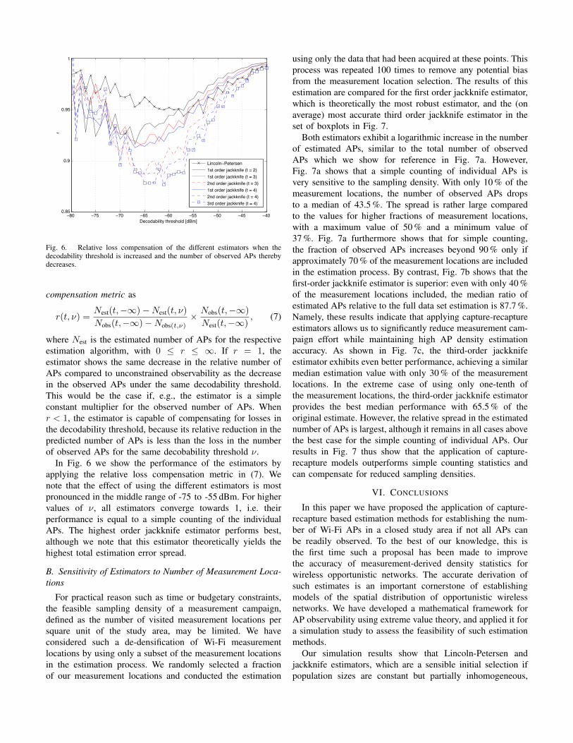
Fig. 6. Relative loss compensation of the different estimators when thedecodability threshold is increased and the number of observed APs therebydecreases.

compensation metric as

r(t, ν) =Nest(t,−∞)−Nest(t, ν)

Nobs(t,−∞)−Nobs(t,ν)× Nobs(t,−∞)

Nest(t,−∞), (7)

where Nest is the estimated number of APs for the respectiveestimation algorithm, with 0 ≤ r ≤ ∞. If r = 1, theestimator shows the same decrease in the relative number ofAPs compared to unconstrained observability as the decreasein the observed APs under the same decodability threshold.This would be the case if, e.g., the estimator is a simpleconstant multiplier for the observed number of APs. Whenr < 1, the estimator is capable of compensating for losses inthe decodability threshold, because its relative reduction in thepredicted number of APs is less than the loss in the numberof observed APs for the same decobability threshold ν.

In Fig. 6 we show the performance of the estimators byapplying the relative loss compensation metric in (7). Wenote that the effect of using the different estimators is mostpronounced in the middle range of -75 to -55 dBm. For highervalues of ν, all estimators converge towards 1, i.e. theirperformance is equal to a simple counting of the individualAPs. The highest order jackknife estimator performs best,although we note that this estimator theoretically yields thehighest total estimation error spread.

B. Sensitivity of Estimators to Number of Measurement Loca-tions

For practical reason such as time or budgetary constraints,the feasible sampling density of a measurement campaign,defined as the number of visited measurement locations persquare unit of the study area, may be limited. We haveconsidered such a de-densification of Wi-Fi measurementlocations by using only a subset of the measurement locationsin the estimation process. We randomly selected a fractionof our measurement locations and conducted the estimation

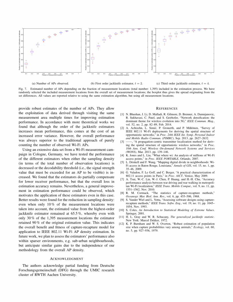
using only the data that had been acquired at these points. Thisprocess was repeated 100 times to remove any potential biasfrom the measurement location selection. The results of thisestimation are compared for the first order jackknife estimator,which is theoretically the most robust estimator, and the (onaverage) most accurate third order jackknife estimator in theset of boxplots in Fig. 7.

Both estimators exhibit a logarithmic increase in the numberof estimated APs, similar to the total number of observedAPs which we show for reference in Fig. 7a. However,Fig. 7a shows that a simple counting of individual APs isvery sensitive to the sampling density. With only 10 % of themeasurement locations, the number of observed APs dropsto a median of 43.5 %. The spread is rather large comparedto the values for higher fractions of measurement locations,with a maximum value of 50 % and a minimum value of37 %. Fig. 7a furthermore shows that for simple counting,the fraction of observed APs increases beyond 90 % only ifapproximately 70 % of the measurement locations are includedin the estimation process. By contrast, Fig. 7b shows that thefirst-order jackknife estimator is superior: even with only 40 %of the measurement locations included, the median ratio ofestimated APs relative to the full data set estimation is 87.7 %.Namely, these results indicate that applying capture-recaptureestimators allows us to significantly reduce measurement cam-paign effort while maintaining high AP density estimationaccuracy. As shown in Fig. 7c, the third-order jackknifeestimator exhibits even better performance, achieving a similarmedian estimation value with only 30 % of the measurementlocations. In the extreme case of using only one-tenth ofthe measurement locations, the third-order jackknife estimatorprovides the best median performance with 65.5 % of theoriginal estimate. However, the relative spread in the estimatednumber of APs is largest, although it remains in all cases abovethe best case for the simple counting of individual APs. Ourresults in Fig. 7 thus show that the application of capture-recapture models outperforms simple counting statistics andcan compensate for reduced sampling densities.

VI. CONCLUSIONS

In this paper we have proposed the application of capture-recapture based estimation methods for establishing the num-ber of Wi-Fi APs in a closed study area if not all APs canbe readily observed. To the best of our knowledge, this isthe first time such a proposal has been made to improvethe accuracy of measurement-derived density statistics forwireless opportunistic networks. The accurate derivation ofsuch estimates is an important cornerstone of establishingmodels of the spatial distribution of opportunistic wirelessnetworks. We have developed a mathematical framework forAP observability using extreme value theory, and applied it fora simulation study to assess the feasibility of such estimationmethods.

Our simulation results show that Lincoln-Petersen andjackknife estimators, which are a sensible initial selection ifpopulation sizes are constant but partially inhomogeneous,

0.3

0.4

0.5

0.6

0.7

0.8

0.9

1

0.1 0.2 0.3 0.4 0.5 0.6 0.7 0.8 0.9 1Fraction of measurement locations

Frac

tion

of e

stim

ated

num

ber o

f APs

w.r.

t. fu

ll lo

catio

n se

t est

imat

e

(a) Number of APs observed.

0.3

0.4

0.5

0.6

0.7

0.8

0.9

1

0.1 0.2 0.3 0.4 0.5 0.6 0.7 0.8 0.9 1Fraction of measurement locations

Frac

tion

of e

stim

ated

num

ber o

f APs

w.r.

t. fu

ll lo

catio

n se

t est

imat

e(b) First order jackknife estimator, t = 2.

0.3

0.4

0.5

0.6

0.7

0.8

0.9

1

0.1 0.2 0.3 0.4 0.5 0.6 0.7 0.8 0.9 1Fraction of measurement locations

Frac

tion

of e

stim

ated

num

ber o

f APs

w.r.

t. fu

ll lo

catio

n se

t est

imat

e

(c) Third order jackknife estimator, t = 4.

Fig. 7. Estimated number of APs depending on the fraction of measurement locations (total number: 1,395) included in the estimation process. We haverandomly selected the included measurement locations from the overall set of measurement locations; the boxplot thus gives the spread originating from theset differences. All values are reported relative to using the same estimation algorithm, but using all measurement locations.

provide robust estimates of the number of APs. They allowthe exploitation of data derived through visiting the samemeasurement area multiple times for improving estimationperformance. In accordance with more theoretical works wefound that although the order of the jackknife estimatorsincreases mean performance, this comes at the cost of anincreased error variance. However, the overall performancewas always superior to the traditional approach of purelycounting the number of observed Wi-Fi APs.

Using an extensive data set from a Wi-Fi measurement cam-paign in Cologne, Germany, we have tested the performanceof the different estimators when either the sampling density(in terms of the total number of observation locations) isdecreased or the decodability threshold (i.e., the signal strengthvalue that must be exceeded for an AP to be visible) is in-creased. We found that the estimators do partially compensatefor lower receiver performance, but that the overall loss inestimation accuracy remains. Nevertheless, a general improve-ment in estimation performance could be observed, whichmotivates the application of these estimators even in this case.Better results were found for the reduction in sampling density:even when only 10 % of the measurement locations weretaken into account, the estimated value from the highest-orderjackknife estimator remained at 65.5 %, whereby even withonly 30 % of the 1,395 measurement locations the estimatorretained 90 % of the original estimation value. This indicatesthe overall benefit and fitness of capture-recapture model forapplication to IEEE 802.11 Wi-Fi AP density estimation. Infuture work, we plan to assess the estimators’ performance alsowithin sparser environments, e.g. sub-urban neighbourhoods,but anticipate similar gains due to the independence of ourmethodology from the overall AP density.

ACKNOWLEDGMENT

The authors acknowledge partial funding from DeutscheForschungsgemeinschaft (DFG) through the UMIC researchcluster of RWTH Aachen University.

REFERENCES

[1] N. Bhushan, J. Li, D. Malladi, R. Gilmore, D. Brenner, A. Damnjanovic,R. Sukhavasi, C. Patel, and S. Geirhofer, “Network densification: thedominant theme for wireless evolution into 5G,” IEEE Commun. Mag.,vol. 52, no. 2, pp. 82–89, Feb. 2014.

[2] A. Achtzehn, L. Simic, P. Gronerth, and P. Mahonen, “Survey ofIEEE 802.11 Wi-Fi deployments for deriving the spatial structure ofopportunistic networks,” in Proc. 24th IEEE Int. Symp. Personal Indoorand Mobile Radio Commun. (PIMRC), Sep. 2013, pp. 2627–2632.

[3] ——, “A propagation-centric transmitter localization method for deriv-ing the spatial structure of opportunistic wireless networks,” in Proc.10th Ann. Conf. Wireless On-demand Network Systems and Services(WONS), Mar. 2013, pp. 139–146.

[4] K. Jones and L. Liu, “What where wi: An analysis of millions of Wi-Fiaccess points,” in Proc. IEEE PORTABLE, Orlando, 2007.

[5] L. Driskell and F. Wang, “Mapping digital divide in neighborhoods: Wi-Fi access in Baton Rouge, Louisiana,” Annals of GIS, vol. 15, no. 1, pp.35–46, 2009.

[6] G. Valadon, F. Le Goff, and C. Berger, “A practical characterization of802.11 access points in Paris,” in Proc. AICT, Venice, May 2009.

[7] A. Tsui, W.-C. Lin, W.-J. Chen, P. Huang, and H.-H. Chu, “Accuracyperformance analysis between war driving and war walking in metropoli-tan Wi-Fi localization,” IEEE Trans. Mobile Comput., vol. 9, no. 11, pp.1551–1562, Nov. 2010.

[8] R. M. Cormack, “The statistics of capture-recapture methods,”Oceanogr. Mar. Biol. Ann. Rev., vol. 6, pp. 455–506, 1968.

[9] S. Vander Wiel and L. Votta, “Assessing software designs using capture-recapture methods,” IEEE Trans. Softw. Eng., vol. 19, no. 11, pp. 1045–1054, Nov. 1993.

[10] S. Coles, An Introduction to Statistical Modeling of Extreme Values.Springer, 2001.

[11] H. L. Gray and W. R. Schucany, The generalized jackknife statistic.New York: Marcel Dekker, 1972.

[12] K. P. Burnham and W. S. Overton, “Robust estimation of populationsize when capture probabilities vary among animals,” Ecology, vol. 60,no. 5, pp. 927–936, 1979.