1

IEEE 802.11ad-based Radar: An Approach to

Joint Vehicular Communication-Radar System

Preeti Kumari, Junil Choi, Nuria Gonzalez-Prelcic, and Robert W. Heath Jr.

Abstract

Millimeter-wave (mmWave) radar is widely used in vehicles for applications such as adaptive cruise

control and collision avoidance. In this paper, we propose an IEEE 802.11ad-based radar for long-range

radar (LRR) applications at the 60 GHz unlicensed band. We exploit the preamble of a single-carrier (SC)

physical layer (PHY) frame, which consists of Golay complementary sequences with good correlation

properties, as a radar waveform. This system enables a joint waveform for automotive radar and a

potential mmWave vehicular communication system based on IEEE 802.11ad, allowing hardware reuse.

To formulate an integrated framework of vehicle-to-vehicle (V2V) communication and LRR based on

a mmWave consumer wireless local area network (WLAN) standard, we make typical assumptions for

LRR applications and incorporate the full duplex radar assumption due to the possibility of sufficient

isolation and self-interference cancellation. We develop single- and multi-frame radar receiver algorithms

for target detection as well as range and velocity estimation within a coherent processing interval. Our

proposed radar processing algorithms leverage channel estimation and time-frequency synchronization

techniques used in a conventional IEEE 802.11ad receiver with minimal modifications. Analysis and

simulations show that in a single target scenario, a Gbps data rate is achieved simultaneously with

cm-level range accuracy and cm/s-level velocity accuracy. The target vehicle is detected with a high

probability of detection (>99.9%) at a low false alarm of 10−6 for an equivalent isotropically radiated

power (EIRP) of 43 dBm up to a vehicle separation distance of 200 m.

Preeti Kumari and Robert W. Heath Jr. are with the Wireless Networking and Communications Group, the University of Texasat Austin, TX 78712-1687, USA (e-mail: {preeti kumari, rheath}@utexas.edu). J. Choi is with the Department of ElectricalEngineering, POSTECH, Pohang, Gyeongbuk, Korea 37673 (e-mail:junil@postech.ac.kr). Nuria Gonzalez-Prelcic is with theDepartment of Signal Theory and Communications, Universidade de Vigo, Vigo, Spain 36310 (email: nuria@gts.uvigo.es) Thisresearch was partially supported by the U.S. Department of Transportation through the Data-Supported Transportation Operationsand Planning (D-STOP) Tier 1 University Transportation Center and by the Texas Department of Transportation under Project0-6877 entitled “Communications and Radar-Supported Transportation Operations and Planning (CAR-STOP)”. This work wasalso supported by a gift from National Instruments.

arX

iv:1

702.

0583

3v1

[cs

.IT

] 2

0 Fe

b 20

17

2

I. INTRODUCTION

Vehicular radar and communication are the two primary means of using radio frequency

(RF) signals in transportation systems. Automotive radars provide high-resolution sensing using

proprietary waveforms in the mmWave band [1, Ch. 4]. They enable safety- and comfort-related

functions, such as adaptive cruise control, blind spot warning, and pre-crash applications [2].

Vehicular communication allows vehicles to exchange safety messages or raw sensor data for

applications such as forward collision warning, do-not-pass warning, and cooperative adaptive

cruise control [3]. The default vehicular communication standard is dedicated short-range com-

munication (DSRC), which is designed for low-latency using a WLAN-based physical layer

and is allocated 75 MHz of licensed spectrum in the 5.9 GHz band [4]. Unfortunately, DSRC

achieves data rates of at most 27 Mbps, much less than the requirement for applications such as

full automated driving (based on raw sensor data exchange to enlarge sensing range), or precise

navigation (based on downloading high-definition 3D maps), which require Gbps data rates [5].

A solution to realize the next generation of high data rate connected vehicles is to exploit the

large bandwidths available in the mmWave spectrum. This could be achieved using a 5G solution,

a 60 GHz unlicensed solution, or a proprietary waveform in dedicated spectrum [6]. Additionally,

it is not only interesting to achieve higher data rates in vehicular communications, but it is

also beneficial to have a joint communication and radar system that allows hardware reuse.

In the past half-decade, a number of joint communication-radar systems have been proposed

(see, e.g., [7] and the references therein). These approaches can be mainly classified as either a

simultaneous system or a non-simultaneous system. In a simultaneous system, a single-carrier

[8], [9] or a multi-carrier waveform [9]–[11] are used for both communication and radar at the

same time. In a non-simultaneous system, radar and communication operate in different time

intervals [12], [13]. Most of the prior work [7]–[10], [12], [13] used waveforms that are not

based on a communication standard.

OFDM waveforms are popular for implementing simultaneous joint communication-radar

systems at sub-6 GHz frequencies [9]–[11]. In [9], the radar parameters are estimated by

leveraging the channel estimation technique for OFDM communication systems, where the

samples obtained at the output of the OFDM communication receiver before channel equalization

is divided by the known transmitted data symbol to obtain the DFT of the channel coefficients.

In [10], radar parameters are estimated using classical correlation-based (matched filter) radar

3

processing approaches that exploit OFDM baseband signals. The independence of the estimated

channel coefficients from the transmitted data in [9] allows a higher dynamic range (between the

strongest and the weakest reflection) as compared to [10], without sacrificing processing gain and

resolution. The sidelobe levels in [9], however, are not ideal for radar ranging. In [11], the IEEE

802.11p V2V communication standard was analyzed as in [9] for automotive radars. The IEEE

802.11p-based radar, however, cannot achieve cm-level range and cm/s-level velocity resolution,

which are desirable in automotive radars [2], due to insufficiently low bandwidth. OFDM-

based simultaneous systems also suffer from a high peak-to-average power ratio (PAPR), unlike

traditional automotive radars with frequency modulated continuous wave (FMCW) waveform

that has PAPR of 0 dB.

In this paper, we propose a mmWave joint vehicular communication and radar system. We build

our approach around the IEEE 802.11ad mmWave WLAN standard, reusing the same waveform

for automotive radar. This allows us to exploit the same spectrum and to leverage shared hardware

based on the mmWave consumer WLAN standard. The approach is reasonable because the most

prevalent vehicular communication standard, DSRC, is based on a WLAN standard. The use of a

standard mmWave waveform, which provides access to a large bandwidth, will lead to significant

advantages in terms of higher data rates for communication and better accuracy/resolution for

radar operation compared with approaches based on sub-6 GHz frequencies. The integration of

cooperative communication approaches and autonomous radar sensing solutions will improve the

system performance in automotive safety and efficiency applications due to the mutual exchange

of complementary information (e.g., enhancing the radar imaging accuracy [14] or reducing

beam training overhead for communications [5]). The joint system will also lead to a potential

increase in the penetration rate of mmWave communication in vehicles and enhanced security

[15].

In this initial study of IEEE 802.11ad-based radar, we make several typical assumptions for

LRR applications: 1) a target vehicle can be represented by a single point model [16] and 2) the

location, velocity, and radar cross section of a target vehicle remain constant during a coherent

processing interval (CPI) [17]. We also assume full-duplex radar operation due to sufficient

isolation and self-interference cancellation provided by the spacing between the TX and the RX

arrays, use of efficient circulators [18], TX/RX beamforming [19], and the possibility of further

suppression in the digital, analog-circuit, or antenna domains [20]. These assumptions are further

described in Section III.

4

The main contributions of this paper are summarized as follows.

• A system model is proposed for joint vehicle-to-vehicle communication and long-range

radar using the SC PHY frame of IEEE 802.11ad. It captures the nuances of the channel

description for both communication and radar systems along with the signal model for

WLAN-based transmitter and receiver.

• Single- and multi-frame radar algorithms are developed for single- and multi-target detection

as well as range and velocity estimation. These algorithms exploit the IEEE 802.11ad

preamble and leverage conventional WLAN time-frequency synchronization and channel

estimation techniques per frame.

• Simulations are performed to evaluate the performance of the proposed joint communication-

radar system, which meets the required LRR specifications [2], [21]. In a single target

scenario, we achieve a Gbps communication data rate simultaneously with the cm/s-level

velocity accuracy using multiple frames (in a CPI > 0.06 ms) and the cm-level range

accuracy using a single frame. The velocity and range accuracy is measured quantitatively

using root MSE. The target is detected with a high probability of detection (> 99.9%) at

a significantly low false alarm rate of 10−6 up to a range of 200 m [21]. In a multi-target

situation, we can achieve a range resolution of < 0.1 m and a velocity resolution of < 0.6

m/s using multiple frames in a 4.2 ms CPI, which is less than CPI duration typically used

for LRR processing (e.g., [17] uses a CPI of 10 ms).

• Theoretical performance analysis using the Cramer-Rao lower bound (CRLB) is provided for

the single-frame target range and velocity estimation algorithms following the approach in

[22, Ch. 7]. The CRLB is derived for the velocity estimation using multiple IEEE 802.11ad

SC PHY frames in a single target scenario with additive Gaussian clutter-plus-noise. In

numerical simulations, we achieve the velocity MSE very close to its CRLB. The single-

frame range estimation MSE is quite close to its CRLB and the slight difference between

them, which is less than 2 cm2, is due to the limited accuracy of the employed WLAN

symbol synchronization techniques [23], [24].

Our previous work in [25] was the first to propose the idea of using IEEE 802.11ad for a

joint vehicular communication and radar system. There were some limitations in [25] that are

overcome in this paper. First, the system model was developed only for a single target model

using a single frame. It did not include a multi-target model or a false alarm rate detection

5

Table I: Frequently Used Symbols

Notation Description

Ts Symbol period

Es Signal energy per symbol at the transmitter

T CPI duration

M Number of frames in a CPI

τp Round-trip delay of the pth target

ρp Range of the pth target

νp Doppler shift of the pth target

vp Relative radial velocity of the pth target

ζrad SCNR of the received radar signal

performance metric. Second, the Doppler shift estimation was not accurate at low and medium

signal-to-noise ratio (SNR). Third, it did not provide a theoretical insight into the performance.

Our new work overcomes these limitations and provides a further in-depth analysis and simulation

of the proposed IEEE 802.11ad-based communication-radar system.

The rest of the paper is organized as follows. A summary of the preamble sequences for an

SC PHY frame of IEEE 802.11ad is presented in Section II. In Section III, an integrated system

model of LRR and V2V communication is developed. Section IV proposes different single- and

multi-frame processing techniques and analyzes their theoretical performance for radar parameter

estimation. Numerical results and performance evaluations are described in Section V, while the

conclusion follows in Section VI.

Notation: We use the following notation throughout the paper: vectors are denoted by boldface

lowercase letters a, matrices by boldface capital letters A, and scalar values by a, A. The nth

component of vector a is written as a[n] and the (`,m)th element of matrix A is denoted by

A[`,m]. We use the notation |c| for the magnitude of c, ∠c for the phase of c, and a(t)∗ b(t) for

the convolution between signals a(t) and b(t). ||B||F is the Frobenius norm, B∗ is the conjugate

transpose, BT is the transpose, and Bc is the conjugate of matrix B. We use the notation

NC(µ, σ2) to denote a complex circularly symmetric Gaussian random variable with mean µ

and variance σ2. The subscript rad refers to radar, com refers to communication, TX refers to

a transmitter, RX refers to a receiver, c refers to clutter, and n refers to noise. Frequently used

symbols in the paper are summarized in Table I.

6

Figure 1: The structure of the SC PHY IEEE 802.11ad frame, which consists of a preamble, aheader, communication data blocks (BLKs) and optional beam training fields. The preamble hasmany repeated sequences with good correlation properties that makes it suitable for radar.

-a128-b128 b128 -a128-b128a128-a128 -b128 -b128

a512 b512

a256 b256

Figure 2: Extracted CEF for an SC PHY frame. It contains a 128 sample Golay complementarypair, denoted by [a128 b128], a 256 sample Golay complementary pair, denoted by [a256 b256],and a 512 sample Golay complementary pair, denoted by [a512 b512].

II. THE IEEE 802.11AD PREAMBLE

In this section, we review the preamble of the IEEE 802.11ad SC PHY frame and compute

its ambiguity function to assess its suitability as an automotive radar waveform for single- and

multi-target vehicular scenarios.

A. Frame Structure

An IEEE 802.11ad SC PHY frame structure is shown in Fig. 1. In this paper, we exploit the

preamble, which is composed of the short training field (STF) and the channel estimation field

(CEF). The preamble in the SC PHY frame is similar to that in other PHY frames of IEEE

802.11ad [26]. Therefore, the findings using SC PHY modulation can be extended to other PHY

preambles.

The STF is composed of sixteen repeated 128 sample Golay complementary sequence, a128,

followed by its binary complement −a128 [26]. It is used in communication for frame synchro-

nization and frequency offset estimation. The frame synchronization algorithm can be leveraged

for range estimation and the frequency offset estimation technique can be used for velocity

estimation of a radar target, as explained in Section IV.

The CEF consists of a 512 sample Golay complementary pair, denoted by [a512 b512] and

is followed by −b128, as shown in Fig. 2. It is used to estimate the communication channel

parameters. The channel estimation algorithm can also be leveraged for target range and velocity

estimation. In this paper, we propose radar algorithms for target detection as well as range and

7

Am

plit

ud

e

ν TP τ/T

s

01.2 -150

1 -100

0.2

0.8 -50

0.4

0.6 00.4 50

0.6

0.2 1000 150

0.8

1

Figure 3: Ambiguity function diagram of the 512 sample Golay complementary pair with durationTp. Here, τ denotes delay, Ts represents symbol period, ν denotes Doppler shift, and Tp = 512Ts.

velocity estimation by using both the STF and the CEF, either jointly or by using the CEF after

the STF, as explained in Section IV. The algorithms that exploit the STF and the CEF jointly can

be used for a longer range of operation as compared to the one that uses the CEF after the STF.

The algorithms that use the CEF after the STF, however, leverage the perfect auto-correlation

property of Golay complementary sequences desirable in automotive radars.

B. Ambiguity Function

To establish the suitability of the IEEE 802.11ad preamble for automotive radar, we use the

ambiguity function. The ambiguity function diagram of [a512 b512] is computed using the closed

form solution in [27] and is shown in Fig. 3. The zero-Doppler cut of the ambiguity function

indicates that [a512 b512] has a perfect auto-correlation with no sidelobe along the zero-Doppler

axis. This characteristic makes it ideal for radar target detection, which does not exist in FMCW

signals typically used in LRR [28]. The ambiguity function of [a512 b512] also depicts that it is

less tolerant to large Doppler shifts. These sequences, however, are still acceptable for LRR due

to the small normalized Doppler shift inherent in the vehicular environment.

III. SYSTEM MODEL

In this section, we formulate the signal and channel models for the proposed vehicular

communication and automotive radar system. We consider the use case where a source vehicle

8

Source Vehicle Recipient / Target Vehicle

Mainlobe of Communication TX-beam

Stationary Clutter(Reflections from

Trees)

Target Vehicle

Stationary Clutter(Reflections from

Road)

Figure 4: Illustration of a vehicular scenario, where a source vehicle transmits an IEEE 802.11adsignal to a recipient vehicle receiver and uses the echoes from target vehicles and clutter to derivetarget range and velocity estimates at the IEEE 802.11ad-based radar receiver mounted on thesource vehicle.

sends an IEEE 802.11ad waveform to a recipient vehicle receiver and uses the echoes from a

single or multiple target(s) to derive range and velocity estimates, as shown in Fig. 4. We assume

a multiple-antenna system for the joint communication-radar with an NTX-element transmit

(TX) antenna array mounted on the source vehicle, and an NRX-element receive (RX) antenna

array mounted on both the source and recipient vehicles. First, we develop the signal model

for the IEEE 802.11ad waveform at the source vehicle, which serves as the TX signal for

both communication and radar systems simultaneously. Second, we describe the one-way V2V

communication channel and the two-way single and multi-target LRR channels at the mmWave

band. Finally, we develop signal models for the communication receiver at the recipient vehicle

and the radar receiver at the source vehicle.

A. Transmit Signal Model

The complex baseband continuous-time representation of the IEEE 802.11ad waveform is

x(t) =√Es

∞∑n=−∞

s[n]gTX(t− nTs), (1)

where Es is the signal energy per symbol at the transmitter, gTX(t) is the unit energy TX pulse-

shaping filter, Ts is the sample duration, and s[n] is the transmitted symbol sequence correspond-

ing to a single-carrier waveform of IEEE 802.11ad normalized such that E [|s[n]|2] = 1. The

symbol period Ts ≈ 1/W , where W is the signaling bandwidth. The IEEE 802.11ad specification

defines the RX filter for error vector magnitude (EVM) measurement as a root-raised cosine

9

Source Vehicle

One-way Distance (ρ0)

Communication RXBeamforming

(𝜙0, θ0)

TXBeamforming

TX Antenna Array

x(t)

NRX

RX Antenna Array

ycom(t)

Recipient Vehicle

Relative Velocity (v0)

NTX

(𝜙0, θ0)

(a) One-way communication channel. Here, ycom(t) denotes the continuous-time receivedcommunication signal.

RX Combining

RX Antenna Array

Source Vehicle

Target Vehicle Echoes

Target (Recipient) Vehicle

Round-trip Distance (2ρ0)

Relative Velocity (v0)

y(t)NRX (𝜙0, θ0)

(b) Two-way radar channel for a single target vehicle, where the scattering centers of therecipient vehicle fall within a single radar resolution and are represented by a point target.

Here, y(t) denotes the continuous-time received radar signal.

Figure 5: After the IEEE 802.11ad beam alignment, the TX and RX beams at the source vehicleare pointed towards the recipient vehicle.

(RRC) filter with a roll-off factor of 0.25, but a specific TX pulse shaping is not specified.

Therefore, in numerical simulations, we have assumed a unit energy RRC waveform with the

same roll-off factor for the TX pulse shaping filter gTX(t) and the RX pulse shaping filter gRX(t).

IEEE 802.11ad supports multiple antenna communication with a single data stream. Spatial

multiplexing as found in IEEE 802.11n/ac is not supported. To develop a single data stream

beamforming model, we incorporate the TX/RX analog beamforming vectors into the baseband

model even though the actual beamforming may happen at an intermediate frequency (IF) or

RF. We assume there is no blockage between the source and recipient vehicles.

We consider a coherent processing interval of T seconds, where the location and velocity of a

target vehicle, such as the recipient vehicle, is assumed to be constant. Therefore, the transmitted

signal at the source vehicle during a CPI is

xTX(t) = fTXx(t), 0 ≤ t ≤ T (2)

10

where fTX ∈ CNTX×1 is the TX frequency-flat analog beamforming vector at the source vehicle.

The vector fTX is time invariant in (2) because we assume the direction of the recipient vehicle

is invariant within a CPI.

B. Channel and Target Models

The mmWave channel consists of contributions from a few scattering clusters [29] (such as

reflections from the target vehicles and clutter) and from self- and inter-user interference. We use

two-dimensional (2D) TX/RX antenna arrays at the source and the recipient vehicles because it

will allow high-resolution beamforming in the azimuth and elevation directions and is used in

mmWave communications (see, e.g., [30]) and automotive radars [31]. This will enable a large

beamforming gain, mitigate inter-user interference, increase communication system capacity, and

enhance resolution for radar sensing. In particular, we use uniform planar array (UPA) antennas

with steering vector a(φ, θ) in azimuth angle φ and elevation angle θ. UPAs are being considered

in mmWave system design because of their high space efficiency acquired by placing antennas

on a 2D grid (see, e.g., [32]).

The TX and RX antenna arrays on the source vehicle are closely separated such that both arrays

will see the same location parameters (e.g., azimuth/elevation angle and range) of a scatter. At

the same time, the separation between the TX and the RX antenna arrays at the source vehicle

along with the use of self-interference cancellation mechanism, TX/RX beamforming and an

efficient circulator (e.g., [18]) will provide enough isolation and cancellation for full-duplex

operation. Developing algorithms for full-duplex operation (e.g. self-interference mitigation in

wireless-propagation-domain, analog-circuit-domain, and digital domain [20]) is a subject of

future work. We also assume that the IEEE 802.11ad medium access control protocol will avoid

the inter-user interference from other vehicles.

During the mmWave joint communication-radar operation between the source and recipient

vehicles, we assume that the 3-dB beamwidths of their TX and RX beams are narrow (as in

[30], [33]). We also assume that the beams are steered towards each other without any blockage.

Although very narrow beams will lead to less clutter [34, Ch. 7], low interference [35], and

long range operation due to large beamforming gain, they can yield poor performance with

vehicle mobility and blockage [35], [36]. In [36], the trade-offs between the Doppler effect and

the pointing error when choosing the beam width for mmWave vehicular communications have

been studied, and it has been concluded that the beams must be pointy but not too narrow. Hence,

11

we assume that the TX/RX beams are narrow enough to meet the link budget requirement of

V2V communication and radar but are wide enough to illuminate all the scattering centers of a

far target vehicle within their resolution (similar to the LRR beams defined in [2]). Therefore, we

represent the recipient vehicle as a single point target, as in [16], [28], and model the mmWave

communication channel with a dominated LOS path corresponding to the recipient vehicle.

During a CPI, we assume that the recipient vehicle has an arbitrary range of ρ0 and az-

imuth/elevation direction pair of (φ0, θ0) moving with a relative radial velocity v0 with respect

to (w.r.t) the source vehicle, as shown in Fig. 5. We also assume that the acceleration and the

relative velocity of the recipient vehicle w.r.t the source vehicle is small enough to allow for

constant velocity and quasi-stationary assumption for a CPI, that is, constant v0, ρ0, and (φ0, θ0)

[22, Ch. 2], [17].

1) Communication Channel Model: To evaluate the trade-off between the communication

data rate and radar estimation accuracy, we consider a single target scenario for simplicity.

Assuming the recipient vehicle is the only dominant direct path scatter present in the radar

channel, we model the one-way LOS dominant mmWave communication channel as a frequency-

flat Rician channel [6]. This can be similarly extended to multi-target scenario by including

frequency-selective communication channel model [29]. We assume that the channel is time-

invariant during a single frame because the source and target vehicles are slow enough. We do

not include band-limited filters in the channel model and instead include them in the TX/RX

signal models. Additionally, the timing synchronization is considered in the received signal

model (see Section III-C). The one-way LOS dominated small-scale communication channel

corresponding to the mth frame in a CPI is represented as [37]

Hcom[m] =

(√Jcom

Jcom + 1HLOS[m] +

√1

Jcom + 1Hw[m]

), (3)

where Jcom is the Rician factor, Hcom[m] ∈ CNRX×NTX , and E [||Hcom[m]||2F] = NTXNRX. The

LOS channel matrix, HLOS[m], is expressed as

HLOS[m] = α0ej2πν0mKmTsaRX(φ0, θ0)a

∗TX(φ0, θ0), (4)

where α0 is unit magnitude and fixed phase, aTX(φ0, θ0) denotes the TX steering vector at the

source vehicle, aRX(φ0, θ0) is the RX steering vector at the recipient vehicle, ν0 = 2v0/λ denotes

the Doppler shift, and λ represents the carrier wavelength. The DoA is same as the DoD in (4)

12

because we consider the LOS channel. The elements of Hw[m] are modeled by independent

and identically-distributed (IID) complex Gaussian random variables with zero-mean and unit

variance. We assume that the source and recipient vehicles align their TX/RX beams toward each

other using the IEEE 802.11ad beam training protocol. For the model in (3), the TX beamforming

vector, fTX, at the source vehicle and the RX beamforming vector, fRX,com, is chosen so that the

beamforming gain is maximized [38]. A particular TX/RX codebook is not specified in the IEEE

802.11ad standard. In numerical simulations, we adopt discrete Fourier transform (DFT)-based

codebooks, which have been proposed for the practical implementations of mmWave WLAN

systems [38]. Since the mmWave communication channel is LOS dominated, we assume that

once the link has been established, the TX beam of the source vehicle and the RX beam of the

recipient vehicle is assumed to be pointing towards (φ0, θ0) with a small beam alignment error

[39], as shown in Fig. 5.

The effective complex communication channel model after the TX/RX beamforming is ex-

pressed as

hcom[m] =√Gcomf

∗RX,comHcom[m]fTX, (5)

where Gcom is the large-scale communication channel gain at the recipient vehicle. We use

the close-in (CI) free space reference distance path loss model with CI free space reference

distance of 1 m to model Gcom, which leads to Gcom = λ2/(4π)2ρPL0 [29]. The exponent PL

denotes the path loss (PL) exponent and is close to 2 for mmWave LOS outdoor urban [29]

and rural channels [40]. The actual value of PL, however, will depend on the specific vehicular

scenario. In numerical simulations, we have studied the effect of PL on radar and communication

performance.

2) Target and Clutter Model: We model the mmWave radar channel for a single CPI using

the doubly selective (time- and frequency-selective) model, which is used in automotive radar

systems such as [41]. The radar channel is assumed to be a sum of the contributions from a

few Np dominant direct path target echoes and multi-path spread-Doppler clutter. Each path

corresponding to the pth target echo is described by six physical parameters: its azimuth and

elevation angle of arrival (AoA)/angle of departure (AoD) pair (φp, θp), round-trip delay, τp,

small-scale complex channel gain βp, large-scale channel gain Gp, and Doppler shift νp. The

round-trip delay and Doppler shift corresponding to the pth target echo is related to its distance

ρp and relative velocity vp as τp = 2ρp/c, and νp = 2vp/λ, where c is the speed of light.

13

We represent the radar target model for the co-located TX/RX antenna arrays at the source

vehicle as [42]

Ht(t, f) =

Np−1∑p=0

√Gpβpe

j2πνpte−j2πτpfArad(φp, θp), (6)

where Arad(φp, θp) = acRX(φp, θp)a

∗TX(φp, θp). The large-scale radar channel gain is assumed

to follow free-space path-loss model with PL exponent of 2 (as used extensively in previous

work, e.g., [28]), i.e., Gp = λ2σRCS,p/(64π3ρ4p), where σRCS,p is RCS corresponding to the pth

target. In (6), we only consider far target whose ρp is large compared to the distance change

during the CPI, i.e., ρp � vp/T . Hence, we assume constant βp [17]. We have not included the

band-limiting filters in (6) because they have been taken care in the TX signal model in (1). In

the case of Np = 1, (6) will represent a single-target model and for Np > 1, (6) will represent a

multi-target model. Specifically, we focus on the physical parameters of the 0th path representing

the direct path between the source and recipient vehicles for both single- and multi-target models.

Therefore, the two-way radar channel with the multi-path spread-Doppler clutter matrix,

Hc(t, f), is represented as

Hrad(t, f) = Ht(t, f) + Hc(t, f), (7)

where Hc(t, f) is assumed to be an IID complex Gaussian distributed random process because

of constant TX/RX beamforming vectors (non-scanning mode) during a CPI [34, Ch. 2 and 7].

This assumption is also used in automotive radar algorithms, such as [16], [43]. If the clutter

component is not Gaussian, space-time adaptive processing can be used as a preprocessing step

to filter out the clutter component [44]. The distribution of the elements of Hc(t, f) impacts the

choice of algorithm and performance bounds for radar detection and parameter estimation.

We assume that at both the source and recipient vehicles, the same IEEE 802.11ad-based

beamforming codebook is used. The AoA pair at the radar receiver mounted on the source

vehicle and the AoA pair at the communication receiver mounted on the recipient vehicle is

the same for the direct path between the source and the recipient vehicles, as shown in Fig. 5.

Therefore, it is reasonable to assume that the radar RX beamforming vector, fRX,rad, at the source

vehicle with the target vehicle model in (6) and the communication RX beamforming vector,

fRX,rad, at the recipient vehicle with the LOS channel matrix in (4) satisfies fRX,rad = f cRX,com.

This assumption will enable us to compare the received power between the radar receiver at the

14

source vehicle and the communication receiver at the recipient vehicle.

After the TX/RX beamforming, the effective target model is ht(t, f) = f∗RX,radHt(t, f)fTX

and the effective clutter model is hc(t, f) = f∗RX,radHc(t, f)fTX. In particular, the effective multi-

target model is non-linearly dependent on the physical parameters, making it difficult to analyze

and estimate the multi-target parameters. The target delays and Doppler shifts during a CPI,

however, can be well approximated using the linear counterpart of ht(t, f), known as the 2D

delay-Doppler map, Hmap[`, d] [22, Ch. 7]. The delay-Doppler map partitions the Np paths into

a 2D resolution cell of size ∆τ ×∆ν, where ∆τ = 1/W and ∆ν = 1/T . Assuming τmax is the

maximum delay spread and νmax is the maximum Doppler spread during the CPI, the maximum

number of delay resolution bins is L = dWτmaxe + 1 and the maximum number of resolvable

(one-sided) Doppler shifts is D = dTνmax/2e. Therefore, instead of representing the channel

using continuous delay and Doppler, the delay-Doppler map is represented by uniform spaced

delays τ` = `/W , and Doppler shifts νd = d/T . The virtual delay-Doppler map representation of

ht(t, f) uniformly sampled in delay and Doppler dimensions commensurate with the resolution

in their respective dimensions is given by [37]

ht(t, f) ≈L−1∑`=0

D∑d=−D

Hmap[`, d]e−j2π`Wfej2π

dTt. (8)

We apply classical low-complexity pulse-Doppler algorithms on the 2D delay-Doppler map

obtained during a CPI to estimate target delays and Doppler shifts [22, Ch. 7], as explained later

in Section IV.

C. Received Signal Model

We consider a coherent processing interval of duration T seconds containing M frames. For

simplicity, we assume each frame in the CPI consists of K samples meaning that the data

payload is of the same size. This will allow us to leverage the range and velocity estimation

algorithms of a classic pulse-Doppler radar, which has a constant pulse repetition frequency,

for developing multi-frame IEEE 802.11ad-based radar processing techniques. This assumption

also simplifies the received signal model. The assumption holds true when the communication

system uses maximum frame length for a given channel delay and Doppler spread during high

data transmission load scenario. The radar processing techniques, however, can be extended for

different frame lengths within a CPI.

15

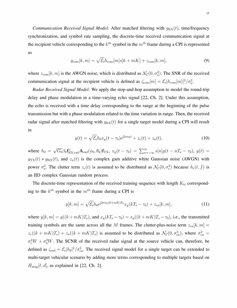
Communication Received Signal Model: After matched filtering with gRX(t), time/frequency

synchronization, and symbol rate sampling, the discrete-time received communication signal at

the recipient vehicle corresponding to the kth symbol in the mth frame during a CPI is represented

as

ycom[k,m] =√Eshcom[m]s[k +mK] + zcom[k,m], (9)

where zcom[k,m] is the AWGN noise, which is distributed as NC(0, σ2n). The SNR of the received

communication signal at the recipient vehicle is defined as ζcom[m] = Es|hcom[m]|2/σ2n.

Radar Received Signal Model: We apply the stop-and-hop assumption to model the round-trip

delay and phase modulation in a time-varying echo signal [22, Ch. 2]. Under this assumption,

the echo is received with a time delay corresponding to the range at the beginning of the pulse

transmission but with a phase modulation related to the time variation in range. Then, the received

radar signal after matched filtering with gRX(t) for a single target model during a CPI will result

in

y(t) =√Esh0xg(t− τ0)ej2πν0t + zc(t) + zn(t), (10)

where h0 =√G0β0f

∗RX,radArad(φ0, θ0)fTX, xg(t − τ0) =

∑∞n=−∞ s[n]g(t − nTs − τ0), g(t) =

gTX(t) ∗ gRX(t), and zn(t) is the complex gain additive white Gaussian noise (AWGN) with

power σ2n. The clutter term zc(t) is assumed to be distributed as NC(0, σ2

c ) because hc(t, f) is

an IID complex Gaussian random process.

The discrete-time representation of the received training sequence with length Ktr correspond-

ing to the kth symbol in the mth frame during a CPI is

y[k,m] =√Esh0ej2πν0(k+mK)Tsxg(kTs − τ0) + zcn[k,m], (11)

where y[k,m] = y((k+mK)Ts), and xg(kTs− τ0) = xg((k+mK)Ts− τ0), i.e., the transmitted

training symbols are the same across all the M frames. The clutter-plus-noise term zcn[k,m] =

zc((k + mK)Ts) + zn((k + mK)Ts) is assumed to be distributed as NC(0, σ2cn), where σ2

cn =

σ2cW + σ2

nW . The SCNR of the received radar signal at the source vehicle can, therefore, be

defined as ζrad = Es|h0|2/σ2cn. The received signal model for a single target can be extended to

multi-target vehicular scenario by adding more terms corresponding to multiple targets based on

Hmap[`, d], as explained in [22, Ch. 2].

16

Time/Frequency Synchronization

Channel Estimation

RangeEstimation

Velocity Estimation

Target Detection

True

Communication preamble processing per frame

Single- and multi-target radar processingper CPIEstimated

Channel and Round-trip Delay

Parameters

Extracted Preamble

Communication Module Radar Module

Figure 6: The processing techniques for target detection and estimation of range and velocityusing an IEEE 802.11ad-based joint communication-radar system. The processing algorithmsleverage the STF and the CEF of multiple frames in a CPI.

IV. PROPOSED RECEIVER PROCESSING TECHNIQUES FOR ENABLING RADAR FUNCTIONS

We propose an IEEE 802.11ad-based radar receiver at the source vehicle that consists of a

communication module and a radar module, as shown in Fig. 6. We consider three primary types

of processing in the radar module: 1) vehicle detection using a constant false alarm rate algorithm;

2) range estimation using time synchronization techniques; and 3) velocity estimation using

frequency synchronization techniques. The algorithms used in the radar processing module are

developed by extending the communication processing techniques over a single frame to multiple

frames in a CPI. This approach will enable the realization of a joint communication-radar system

using a conventional low-cost IEEE 802.11ad system with minimal receiver modifications.

A. Communication Preamble Processing per Frame

In the communication module, training sequences in the preamble of a single frame are used

for time/frequency synchronizations and channel estimation [23]. This is achieved in several

steps: 1) coarse time synchronization based on preamble detection techniques using the STF; 2)

frequency offset estimation using the STF; 3) fine time synchronization using the CEF symbol

boundary detection and the STF/CEF peak detection techniques; and 4) channel estimation using

the CEF. The accuracy of Doppler shift estimation using a single frame in the communication

module is inaccurate at low SNR due to small Doppler shift and less integration time, as explained

later in Remark 2. Therefore, we estimate the Doppler shift in the radar module using multiple

frames.

For simplicity, we describe the processing techniques of the communication module for a

single target vehicular scenario, which can be extended to a multi-target vehicular situation. The

first step of the training sequence processing is the timing synchronization. Since the round-trip

17

delay of a target vehicle, τ0, is a continuous variable, we can represent it as τ0 = `0Ts + τd,

where `0 is an integer and τd is a fractional symbol delay. Then, (11) can be represented for

0 < k < Ktr as

y[k,m] =√Esh0s[k − `0]g(τ0)e

j2πν0(k+mK)Ts + zISI[k,m] + zcn[k,m], (12)

where, zISI[k,m] =√Esh0

∑n 6=k+mK

s[n]g(((k+mK)−n)Ts−τ0)ej2πν0(k+mK)Ts is the intersymbol

interference (ISI).

We use the energy-based symbol synchronization algorithm to estimate the fractional symbol

delay, τd[m], and then apply a fractional symbol delay correction to mitigate its effect [23], [24].

Since the assumed TX and the RX pulse shaping RRC filters lead to an equivalent filter satisfying

the Nyquist condition, we consider g(nTs) = δ[n]. Therefore, the received signal corresponding

to the mth frame is

ym[k] =√Esh0ej2πν0(k+mK)Tss[k − `0] + zm[k], (13)

where ym ∈ CKtr×1 represents the vector of the received training symbols with ym[k] = y[m, k],

and zm ∈ CKtr×1 represents the residual ISI-plus-clutter-plus-noise vector (i.e., zm[k] is the sum

of zcn[k,m] and the residual ISI after fractional symbol delay correction).

After symbol synchronization, we detect the IEEE 802.11ad frame using the normalized auto-

correlation of the STF, which consists of 16 repeated a128. The `th normalized auto-correlation

corresponding to the mth frame is given by

R1[`,m] =

∑P−1n=0 ym[`− n]y∗m[`− n−ND]√∑P−1

n=0 |ym[`− n]|2√∑P−1

n=0 |y∗m[`− n−ND]|2, (14)

where P = 128 is the length of the training sequence and ND = 128 is the distance between

the consecutive training sequences chosen for correlation. The frame start is detected when

|R1[`,m]| > χSTF for 128 times, where χSTF is a pre-defined threshold and is < 1 [23]. The

frame start detection technique, therefore, uses around 128 × 2 to 128 × 3 samples in the STF

field to confirm the detection. The coarse range estimate of the target vehicle by applying the

preamble start detection technique to the mth frame is given by

ˆ01[m] = inf {` | |R1[`,m]| ≥ χSTF} . (15)

18

The carrier frequency offset (CFO) can be estimated by using the auto-correlation based

algorithm and residual CFO estimation techniques proposed in [23]. For simplicity, we assume

that these algorithms achieve perfect carrier frequency offset compensation.

The fine range estimate of the time-delay can be obtained either by using an amplitude-

based method or a phase-based method. The amplitude-based method estimates the fine time-

delay using the cross-correlation, R2[`,m], between multiple a128 in the STF sequence, which

is expressed as

R2[`,m] =Pr−1∑i=0

P−1∑n=0

a128[n]ym[`+ n+ iP ], (16)

where P = 128, and Pr = 16 is the total number of repetitions of a128 in the STF. The fine-time

delay, ˆ02[m], is estimated by detecting the peak of R2[`,m] and is given by

ˆ02[m] = arg max

`:`∈Z|R2[`,m]|2, (17)

where Z is the set of integers. The amplitude-based fine timing synchronization can also be

similarly performed by applying the peak detection technique on the CEF instead of the STF.

Both the peak detection methods perform well even when SCNR ζrad is low.

The timing synchronization at the mth frame can also be fine tuned by performing phased-

based CEF symbol boundary detection [23]. This method, however, does not perform well in

the presence of Doppler shift at low SNR of the received communication signal.

After the fine time synchronization, we extract the received CEF signal to estimate the channel

using the 512 sample Golay complementary pair. The channel estimate, hm[`], is acquired after

removing the cyclic prefix from the correlation values, γ(ym, `), between the received CEF and

[a512 b512] [45]. Therefore, γ(ym, `) and hm[`] are expressed as

γ(ym, `) =1

2P

(P−1∑n=0

ym[n+ `]a∗512[n] +P−1∑n=0

ym[n+ `+ P ]b∗512[n]

)(18)

and

hm[`] = γ(ym, `+NCP) ` = 0, · · · , P − 1, (19)

where P = 512 and the length of the cyclic prefix NCP = 128.

We assume the channel is time invariant during the CEF because the source and recipient

vehicles are slow enough. Based on the channel model in (7) with a single target, the channel

estimate in (19), which leverages the perfect auto-correlation property of Golay complementary

19

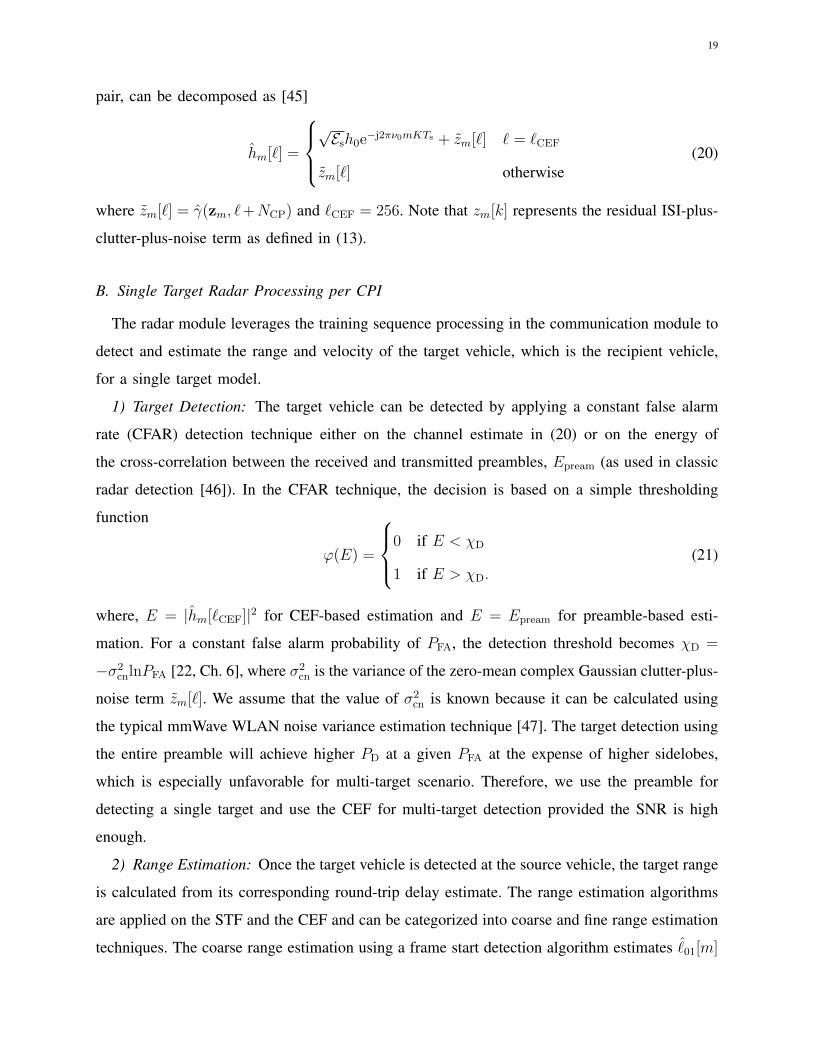
pair, can be decomposed as [45]

hm[`] =

√Esh0e−j2πν0mKTs + zm[`] ` = `CEF

zm[`] otherwise(20)

where zm[`] = γ(zm, `+NCP) and `CEF = 256. Note that zm[k] represents the residual ISI-plus-

clutter-plus-noise term as defined in (13).

B. Single Target Radar Processing per CPI

The radar module leverages the training sequence processing in the communication module to

detect and estimate the range and velocity of the target vehicle, which is the recipient vehicle,

for a single target model.

1) Target Detection: The target vehicle can be detected by applying a constant false alarm

rate (CFAR) detection technique either on the channel estimate in (20) or on the energy of

the cross-correlation between the received and transmitted preambles, Epream (as used in classic

radar detection [46]). In the CFAR technique, the decision is based on a simple thresholding

function

ϕ(E) =

0 if E < χD

1 if E > χD.(21)

where, E = |hm[`CEF]|2 for CEF-based estimation and E = Epream for preamble-based esti-

mation. For a constant false alarm probability of PFA, the detection threshold becomes χD =

−σ2cnlnPFA [22, Ch. 6], where σ2

cn is the variance of the zero-mean complex Gaussian clutter-plus-

noise term zm[`]. We assume that the value of σ2cn is known because it can be calculated using

the typical mmWave WLAN noise variance estimation technique [47]. The target detection using

the entire preamble will achieve higher PD at a given PFA at the expense of higher sidelobes,

which is especially unfavorable for multi-target scenario. Therefore, we use the preamble for

detecting a single target and use the CEF for multi-target detection provided the SNR is high

enough.

2) Range Estimation: Once the target vehicle is detected at the source vehicle, the target range

is calculated from its corresponding round-trip delay estimate. The range estimation algorithms

are applied on the STF and the CEF and can be categorized into coarse and fine range estimation

techniques. The coarse range estimation using a frame start detection algorithm estimates ˆ01[m]

20

with an error of less than 128×3 samples. Fine range estimation based on the symbol boundary

detection or the STF/CEF peak detection and symbol synchronization techniques result in the

delay estimate of ˆ02[m] + τd[m] or ˆ

03[m] + τd[m] with an error of less than 1 sample [23],

which meets the LRR specification of 0.1 m range accuracy [2].

Remark 1. The CRLB bound of the range estimation using the IEEE 802.11ad preamble can be

expressed following the approach in [22, Ch. 7] as

σ2ρ =

c2

8η2W 2Pζrad, (22)

where η depends on the power spectral density shape of x(t) over the preamble duration. We

assume a flat spectral shape of the preamble, which will allow better channel equalization of

the communication system (e.g., Zadoff-Chu sequences used in LTE) and better radar parameter

estimation of the target vehicle (e.g., linear frequency modulated chirp used in automotive radar).

Due to the assumption of flat spectral shape, η2 = (2π)2/12 [22, Ch. 7]. The integration gain P

is equal to the number of preamble symbols used for range estimation, i.e., 16×128 for the fine

range estimation using the STF and 8 × 128 for the fine range estimation using the CEF. The

range estimation CRLB, as can be seen from (22), decreases with the integrated SCNR, which

is defined as Pζrad.

For ζrad > 0 dB and bandwidth W > 1.76 GHz (the exact value of W will depend on chosen

pulse shaping filter), it can be calculated from (22) that it is possible to achieve less than 1 mm

accuracy using a single IEEE 802.11ad frame. In particular, for the RRC pulse shaping filter

that we use in the numerical simulations, the range accuracy is 0.8 mm.

3) Velocity Estimation: The relative velocity of the target vehicle is calculated at the source

vehicle by estimating the Doppler shift of the corresponding target echo. We use the least

squares (LS)-based frequency-offset estimation method over single/multiple frames to estimate

the Doppler shift corresponding to the target vehicle. For this purpose, we choose p ∈ CPM×1

to be a vector of M frames across P delay bins, i.e.,

p =[[y0[k0], · · · , y0[kP−1] · · · yM−1[k0], · · · , yM−1[kP−1]

](23)

where {ki | 0 ≤ i ≤ P − 1} is an index set to the location of the training sequences in each

frame.

21

The Doppler frequency estimation based on the Moose algorithm [48] or the CFO estimation

algorithm used in IEEE 802.11ad [23], when applied on a single frame does not achieve the

desired velocity accuracy of 0.1 m/s due to the small integration time, Tint = PTs, for velocity

estimation, as shown in [25]. Therefore, to achieve desired velocity accuracy, we propose a

multi-frame Moose-based algorithm for the Doppler frequency estimation problem as

ν0 =∠(∑M−1

i=0

∑P−1n=0 p[n+ND + iP ]p∗[n+ iP ]

)2πTD

, (24)

where ND is the distance between two training sequences chosen for correlation and TD is

the time interval between these two training sequences, i.e., NDTs. In the case of multi-frame

velocity estimation, we choose ND = K. In the case of single-frame velocity estimation, we

choose ND = 4× 128. Choosing larger ND improves the estimate, whereas it reduces the range

of offsets that can be corrected, as explained later in Remark 2. The accuracy of frequency-

offset estimation will improve when we use multiple frames (similar to pulse-Doppler radar)

as compared to a single frame (traditionally used in frequency synchronization algorithms of

a standard WLAN receiver) because of larger integration time, Tint = MTD. The length of an

IEEE 802.11ad frame SCPHY frame is variable from 0.002 ms to 1.2 ms [26], whereas CPI of

T = 10 ms [17] and update rate of 10 Hz [1] is used in automotive radar. Therefore, we can

use multiple frames for radar processing, where the number of frames is T/(KTs).

Remark 2. The theoretical performances of the proposed velocity estimation for a single target

vehicle with velocity v in a flat fading channel are summarized as follows.

(a) The CRLB for the velocity estimation using the STF of a single frame, as described in

Appendix A, is

σ2v =

6λ2

(4π)2P 3T 2s ζrad

. (25)

The CRLB expresses a lower bound on the variance of velocity estimators using the STF of a

single frame. If σ2v is above the LRR’s desired MSE for velocity estimation, then it indicates

that the requirement for LRR velocity accuracy cannot be met by any unbiased estimator.

It can be inferred from (25) that the velocity MSE decreases rapidly with an increase in P

and ζrad. The value of P , however, is constant in an SC PHY frame and is equal to 128 ×

16, which implies that CRLB is mainly affected by the change in ζrad.

(b) The CRLB for velocity estimation using preamble across multiple frames for large M , as

22

derived in Appendix A, is

σ2v ≈

6λ2

(4π)2(MP 3 +M3PK2)T 2s ζrad

. (26)

Similar to (25), (26) also suggests that estimated velocity accuracy enhances with the increase

in number of preambles, i.e., MP , and ζrad. Unlike (25), however, (26) adds the flexibility

of increasing the total number of total preamble symbols by choosing higher values of M ,

which improves the accuracy of the velocity estimation.

The extra flexibility in varying M due to the use of multiple frames enables a system trade-

off between target velocity estimation accuracy and communication data rate for the number

of frames within a CPI. The velocity estimation CRLB decreases with an increase in the

total training sequence duration and the numbers of frames within a fixed size CPI, as can

be seen from (26). The number of communication data symbols and consequently data rate,

however, decreases with an increase in the training sequence duration.

(c) Due to the periodicity of the exponential function, the estimate of the Doppler shift calculated

in (24) will only be accurate for

|ν0| ≤1

2NDTs. (27)

In (24), we can use different periodicity of the preamble by choosing different training

sequences. Comparing (25), (26) and (27), however, we infer that there is a trade-off

between accuracy and span of the unambiguous velocity estimation. The multi-frame Doppler

estimation with ND > 128 × 26 has a higher accuracy as compared to the single-frame

Doppler estimation with ND = 512, whereas it has a comparatively reduced range of Doppler

offsets that can be corrected due to larger ND.

C. Multi-target Radar Processing per CPI

In the case of a multi-target model, we use classic pulse-Doppler-based radar processing

technique that leverages the channel estimate derived in (19) to estimate the range and velocity

of multiple targets. First, we obtain an estimate of the delay-Doppler map, Hmap[`, d], where the

`th row of the 2D map, Hmap[`, :], is the M -point DFT of the zero-padded channel estimate vector[h0[`], h1[`], · · · , hM−1[`]

]. Then, we use a thresholding method similar to (21) to detect multiple

targets from the delay-Doppler map [46]. The range of the pth detected target is estimated from

the location of its corresponding delay bin, ˆp, in Hmap[`, d]. Similarly, we determine each target’s

23

velocity from its corresponding Doppler bin dp. We use the channel estimates, which are derived

from the CEF in M frames, for multi-target radar processing because they exploit the desirable

perfect auto-correlation property of the Golay complementary pair.

Remark 3. The range resolution for the multi-target radar processing is ∆ρ = c/(2W ) [49, Ch.

10].

The velocity resolution for multi-target model using conventional Fourier processing is ∆v =

λ/(2Tint), where Tint = MTD with TD = KTs [49, Ch. 10]. This implies that as the number of

frames increases, the resolution of the velocity estimation increases.

For W > 1.76 GHz and T > 4.2 ms, it can be calculated from the theoretical bounds in

Remark 3 that it is possible to achieve less than 8.52 cm range resolution and less than 0.6 m/s

of velocity resolution using the IEEE 802.11ad preamble, which is better than the required LRR

resolution specifications in [2] and typical CPI duration used in automotive radars (see, e.g., 10

ms CPI in [17]). In particular, for the RRC pulse shaping filter that we use in the numerical

simulations, ∆ρ = 7 cm. In numerical results, we show that our proposed joint system and

algorithms achieve these bounds.

V. NUMERICAL RESULTS

In this section, we perform Monte-Carlo simulations with 10,000 trials to evaluate the proposed

radar techniques using IEEE 802.11ad against the required system specifications for LRR in a

typical automotive radar setting [2]. We assume the vehicle radar cross section is 10 dBsm [28].

The multiple-antenna system is assumed to be a UPA with 8 horizontal and 2 vertical elements,

as used in the Qualcomm IEEE 802.11ad chipsets [50]. The 3-dB horizontal beamwidth of the

UPA is 13◦, and the 3-dB vertical beamwidth of the UPA is 60◦.

A. Single Target Automotive Scenario

We simulate the received radar signal for a single target vehicular scenario, where the recipient

vehicle is assumed to be the only target vehicle, as discussed in Section III. We choose the

distance and the relative speed between the target and source vehicles as 50 m and 20 m/s, which

falls in the typical span of LRR range and velocity specifications [2]. We chose fixed location

parameters because the performance bounds of the radar detection and estimation parameters do

not vary with range and relative velocity of the target vehicle, as discussed in Remark-1 and

Remark-2 in Section IV.

24

-32 -30 -28 -26 -24 -22 -20 -18 -16SCNR (dB)

0

0.2

0.4

0.6

0.8

1

Pro

ba

bili

ty o

f D

ete

ction

PFA

= 10-4

PFA

= 10-6

PFA

= 10-8

Figure 7: Probability of detection using different constant false alarm detection rates.

We evaluate the detection performance using probability of detection, PD, for a given proba-

bility of false alarm, which is given by

PD = E[ϕ(E) | target present], (28)

where the thresholding function ϕ(E) is defined in (21). We perform Monte-Carlo simulations

with 10,000 trials to compute PD using the preamble-based detection technique at PFA of 10−4,

10−6, and 10−8. Fig. 7 shows the performance of the proposed detection algorithm as a function

of probability of false alarm and the received SCNR. It indicates that PD grows with increasing

PFA. For a PFA of 10−4, it is possible to achieve radar detection rates greater than 90% above

the received SCNR of -24.3 dB and for a PFA of 10−6, it is possible to achieve PD > 99.9%

for received SCNR > -20.5 dB.

Fig. 8 shows the estimated velocity MSE using the STF of a single frame with P = 128× 16

and ND = 512, and using the preamble of two frames with P = 128×26 and ND = 41, 285. The

estimated velocity MSEs increase linearly (in dB scale) with the SCNR. The velocity estimation

using the LS-based algorithm in (24) is comparatively better than the one proposed in [23]. The

accuracy of the LS-based estimation techniques is very close to its CRLB bound. Using double

frames, we achieve much better velocity estimation accuracy than using a single frame for all

SCNR values. At low SCNR (less than 10 dB), however, even using double frames, we do not

achieve the desired velocity accuracy of 0.1 m/s.

This motivates us to exploit multiple frames as explained in Section IV, which inherently

25

10 20 30 40 50 60 70SCNR (dB)

10-8

10-6

10-4

10-2

100

102

Velo

city M

SE

(m

2/s

2)

[23]LS for single frameCRLB for single frameLS for double framesCRLB for double frames

Figure 8: Estimated velocity MSE using the STF of a single and the preamble of double frames.The MSEs of proposed estimation techniques closely match with their CRLBs.

increases the training sequence and frame duration to better estimate velocity using the LS-

based method. The performance of this algorithm, however, depends on the number of frames

during a CPI. To evaluate the dependence of velocity estimation on the number of frames within

a CPI and investigate its simultaneous effect on the communication system, we consider the

following data rate as the communication performance metric

R =MKCDTs

TE [log2 (1 + ζcom[m])] , (29)

where KCD is the total number of communication data symbols within a frame.

We have performed simulations over different CPI duration at 10 dB SCNR to investigate the

trade-off between velocity estimation MSE and communication data rate, as shown in Fig. 9. For

a fixed CPI duration, the number of frames in a CPI is varied from one to its maximum limit

such that the number of symbols in each frame conforms to the IEEE 802.11ad SC PHY frame

structure. We observe from the simulations that there is a trade-off between the communication

data rate and the velocity estimation accuracy for a given CPI duration with a different number

of frames. With an increase in the number of frames for a fixed CPI duration, the communication

data rate degrades while enhancing the velocity estimation accuracy. We also observe that it is

possible to simultaneously achieve Gbps communication data rate and cm/s-level accurate target

velocity estimation for a CPI of 0.06 ms or more.

In Fig. 10, we compare the performance of various proposed range estimation algorithms and

26

2 10 20 30 40 50 60 70 80Number of frames used for communication data transmission

109

1010

1011

Da

ta R

ate

(b

ps)

(a) Data rate of the IEEE 802.11ad system for a fixed duration of CPI

0.03 ms0.06 ms0.09 ms0.12 ms0.15 ms

2 10 20 30 40 50 60 70 80Number of frames used for velocity estimation

10-5

10-4

10-3

10-2

10-1

Ve

locity M

SE

(m

2/s

2)

(b) MSE of the velocity estimation using multiple frames for a fixed size CPI

0.03 ms0.06 ms0.09 ms0.12 ms0.15 ms

Figure 9: Trade-off between communication data rate and velocity estimation MSE for a fixed sizeCPI. By increasing the duration of training symbols within a CPI, velocity estimation becomesmore accurate with reduced data rate.

the CRLB using a single frame. The desired range MSE for automotive radars is 0.01 m2 [2].

For frame start detection using the STF, we chose a threshold of χ2STF = 1/8 because it reduces

the complexity of the hardware implementation [23]. We observe from Fig. 10 that the fine range

estimation achieves better than the desired accuracy of 0.1 m using the STF/CEF peak detection

for SCNR above 0 dB, and using the CEF symbol boundary detection for SCNR above 6 dB.

The poor performance of range estimation using the CEF symbol boundary detection at low

SCNR can be attributed to the fact the performance of the phase-based estimation is affected by

Doppler shift. The figure also shows that the performance of the frame start detection using the

preamble degrades due to a constant threshold χSTF, which does not adapt to the increasing SCNR

[24]. This does not, however, degrade the performance of the fine range estimation technique.

27

0 2 4 6 8 10 12 14 16 18 20 22

SCNR (dB)

10-8

10-6

10-4

10-2

100

102

104

Ran

ge

MS

E (

m2)

Frame Start Detection Using PreambleSymbol Boundary Detection Using CEFPeak detection Using STFPeak detection Using CEFCRLB

Figure 10: Estimated range MSE for coarse and fine range estimation algorithms using thepreamble of a single frame.

0 50 100 150 200 250ρ

0 (m)

-60

-40

-20

0

20

40

60

80

SC

NR

a

t th

e s

ou

rce

ve

hic

le (

dB

)

-60

-40

-20

0

20

40

60

80

SN

R a

t th

e t

arg

et

ve

hic

le (

dB

)PL exponent 2.5

PL exponent 2.0

PL exponent 2.5

PL exponent 2.0

Figure 11: Received radar SCNR at the source vehicle and received communication SNR at thetarget vehicle as a function of distance between the source and target vehicles.

Indeed, the amplitude-based peak detection techniques using the STF/CEF achieve better than

the desired automotive range accuracy of 0.1 m using a single frame without incorporating

significant complexity. These peak detection techniques achieve range estimation MSEs quite

close to the CRLB with a slight difference of less than 2 cm2 between them. This difference is

due to the fixed oversampling factor used in the symbol synchronization algorithm to estimate

the fractional symbol delay, which can be easily improved using a higher oversampling factor

or by using more complex symbol synchronization algorithm.

Fig. 11 shows the received radar SCNR at the source vehicle and the received communication

28

RX Antenna Arrayat the Source Vehicle

Tv0(𝝳𝜙, 𝝳θ)

Vehicle T

Vehicle RR

Figure 12: A multi-target scenario with two vehicles, namely vehicle R and vehicle T, withinthe mainlobe of the TX beam at the source vehicle. Both the vehicles are slightly separated inrange, relative velocity, and direction w.r.t the source vehicle.

SNR at the target vehicle decrease for a given TX EIRP of 43 dBm (maximum EIRP for USA

[26]) with PL exponents of 2 (as used in automotive radar simulations, e.g., [28], and in mmWave

communication propagation model, e.g., [29]) and 2.5 (as used in [51] for link budget analysis

of IEEE 802.11ad indoor applications) assuming noise figure of 6 dB [51]. We also infer from

Fig. 11 that for a given EIRP, one-way received communication SNR is higher than the two-

way radar SCNR and both of them reduces with the increasing ρ0 due to decreasing large-scale

channel gains Gcom and Grad. Based on Fig. 7 and Fig. 11, we infer that for PL exponent of 2.0,

the IEEE 802.11ad-based radar can detect very reliably with PD > 99.9% and PFA = 10−6 till

200 m, which is desirable for LRR [21]. The span of ρ0 over which the proposed radar system

can detect also overlaps with the range of ρ0 over which we can reliably estimate the cm-level

accurate range and cm/s-level accurate velocity of the target vehicle within a CPI duration of

less than 10 ms, which is desirable in LRR [2], [17].

B. Multi-target Scenario

The performance of the IEEE 802.11ad-based joint communication-radar system is also eval-

uated for a multi-target vehicular scenario, where we use the doubly selective channel model as

described in Section III. To demonstrate the range and velocity resolutions of the joint system, we

consider a two-target vehicle scenario. In this scenario, one of the target vehicles is a recipient

vehicle, say vehicle R. The second target vehicle is considered within the beamwidth of the

source vehicle and is separated in range, relative velocity, and AoA/AoD as compared with the

recipient vehicle by δρ and δv, and (δφ, δθ) respectively, as shown in Fig. 12. For vehicle R,

we choose range as 14.32 m and velocity as 30 m/s, which falls in the typical operating span

29

Figure 13: Mesh plot of the estimated delay-Doppler map. The plot shows two mainlobe peakscorresponding to the simulated vehicle R and vehicle T. Due to the broad mainlobe width in theDoppler domain velocity resolution is limited to around 35 m/s in this simulation.

of LRR range and velocity specifications [2]. We consider that the AoA/AoD corresponding to

the vehicle R is (90◦, 90◦), which is likely to happen when the vehicle R is in the same lane

as the source vehicle for applications such as cruise control. For vehicle T, we consider δρ =

4.26 m, δv = 30 m/s, and (δφ, δθ) = (100◦, 90◦), which also falls in the typical span of LRR

specifications [2].

Figs. 13 and 14 represent the 2D and three-dimensional (3D) plots of the estimated normalized

delay-Doppler map with 10 frames in one CPI of 128000 samples, i.e., 0.072 ms duration.

The normalization is done w.r.t the maximum received power at the source vehicle. The delay

resolution is 0.07 m, and the Doppler resolution is 13750 KHz, calculated from Remark 3. In

both figures, we plot the amplitude of the delay-Doppler map w.r.t the discrete-delay, `, and 1000

times interpolated discrete-Doppler, d, as described in Section III. The delay-Doppler map is

interpolated in the Doppler (slow-time) dimension to visualize the resolution degradation effect

due to the wide mainlobe and high sidelobes of the Doppler response in a given delay bin. These

plots show that vehicle R and vehicle T responses are separated by 50 delay bins, corresponding

to 4.26 m. They also show high sidelobes and wide mainlobe in the Doppler axis resulting in

limited Doppler resolution. From the 3-dB mainlobe width along the Doppler dimension, we

infer that the Doppler resolution is 13,750 KHz and the corresponding velocity resolution is

30

0 1000 2000 3000 4000 5000 6000 7000 80001000*#Doppler Bin

60

80

100

120

140

160

180

200

#D

ela

y B

in

0

0.1

0.2

0.3

0.4

0.5

0.6

0.7

0.8

0.9

1

Figure 14: The estimated 2D-plot of the normalized delay-Doppler map shows that there are2 dominant reflections present in the 118th and 168th delay bins and in the first and secondDoppler bins.

34.375 m/s. The velocity resolution, however, improved to less than 0.6 m/s, when we increased

the CPI duration to more than 4.2 ms, as can also be seen from Remark 3. From the 3-dB

mainlobe width along the delay dimension, we deduce that the range resolution is 7 cm. We can

also infer from Fig. 13 that gain of vehicle R is less than vehicle T. This is because vehicle R

is farther as compared to vehicle T from the source vehicle. This example illustrates the limit

of velocity resolution, which is highly dependent on the duration of a CPI. At the same time, it

also demonstrates the cm-level resolution and ultra-low sidelobes along the range dimension.

VI. CONCLUSIONS

In this paper, we developed a mmWave automotive radar based on the IEEE 802.11ad standard

to enable a joint mmWave vehicular communication-radar system. Our proposed radar receiver

exploits the preamble structure (repeated Golay complementary sequences) of an IEEE 802.11ad

SC PHY frame because of its perfect auto-correlation property at the zero-Doppler shift. We

proposed different single- and multi-frame radar algorithms for the single- and multi-target

radar detection as well as range and velocity estimation by leveraging standard WLAN receiver

algorithms and classical pulse-Doppler radar algorithms. We evaluated the performance of these

algorithms both analytically and by simulations. The target vehicle is detected very reliably at

significantly low constant false alarm rate for SCNR above -20.5 dB. The range of the target

31

vehicle is estimated with higher resolution and accuracy than the minimum requirement of the

LRR specifications (0.5 m range resolution and 0.1 m range accuracy). The velocity estimation

using single frame processing technique met the desired accuracy of 0.1 m/s above 45 dB SCNR,

whereas using multi-frame processing technique achieved velocity accuracy of less than 0.1 m/s

even at SCNR as low as -20.5 dB for a CPI of 4.2 ms. We also achieved the desired velocity

resolution of less than 0.6 m/s for a CPI of 4.2 ms using multi-frame processing. Additionally,

we showed that there is a trade-off between velocity estimation accuracy and communication

data rate for a fixed CPI duration, while the desired velocity accuracy is simultaneously achieved

with Gbps data rate for a CPI of 0.06 ms or more. These results indicate that IEEE 802.11ad-

based joint communication-radar system is a promising option for next-generation automotive

applications. Future work includes modifying the IEEE 802.11ad waveform that permits a trade-

off between radar parameters’ estimation accuracy/resolution and communication data rate to

adjust adaptively to the requirements imposed by different vehicular scenarios.

APPENDIX A

CRAMER RAO LOWER BOUND FOR VELOCITY ESTIMATION

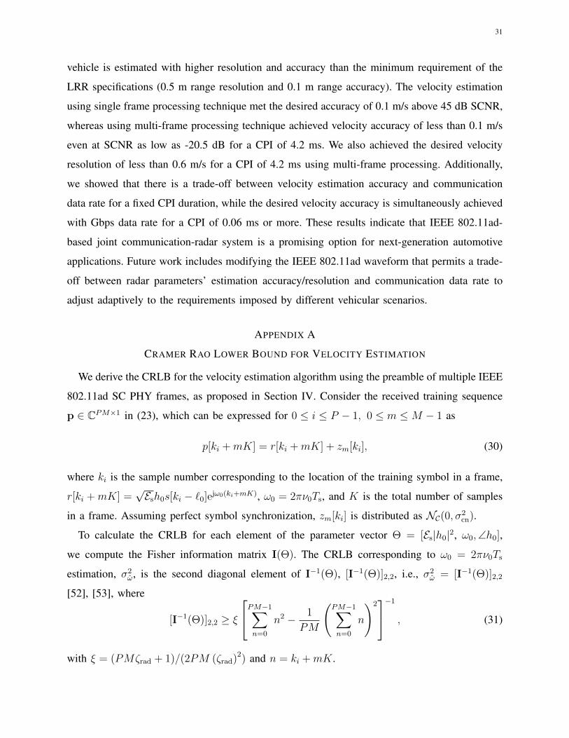
We derive the CRLB for the velocity estimation algorithm using the preamble of multiple IEEE

802.11ad SC PHY frames, as proposed in Section IV. Consider the received training sequence

p ∈ CPM×1 in (23), which can be expressed for 0 ≤ i ≤ P − 1, 0 ≤ m ≤M − 1 as

p[ki +mK] = r[ki +mK] + zm[ki], (30)

where ki is the sample number corresponding to the location of the training symbol in a frame,

r[ki + mK] =√Esh0s[ki − `0]ejω0(ki+mK), ω0 = 2πν0Ts, and K is the total number of samples

in a frame. Assuming perfect symbol synchronization, zm[ki] is distributed as NC(0, σ2cn).

To calculate the CRLB for each element of the parameter vector Θ = [Es|h0|2, ω0,∠h0],

we compute the Fisher information matrix I(Θ). The CRLB corresponding to ω0 = 2πν0Ts

estimation, σ2ω, is the second diagonal element of I−1(Θ), [I−1(Θ)]2,2, i.e., σ2

ω = [I−1(Θ)]2,2

[52], [53], where

[I−1(Θ)]2,2 ≥ ξ

PM−1∑n=0

n2 − 1

PM

(PM−1∑n=0

n

)2−1 , (31)

with ξ = (PMζrad + 1)/(2PM (ζrad)2) and n = ki +mK.

32

For ζrad � (1/P ) and for consecutive samples in a single frame, i.e., M = 1, the CRLB for

estimation of the Doppler shift ν0 in Hz, can be expressed as σ2ν = [I−1(Θ)]2,2/(4π

2T 2s ), which

results in

σ2ν ≥

6

(2π)2T 2s P (P 2 − 1)ζrad

≈ 6

(2π)2P 3T 2s ζrad

. (32)

In case when p is composed of non-consecutive training sequence, i.e., n = i+mK, then for

large number of frames, i.e., large M , we can simplify (31) as

σ2ν ≥

6

4π2(MP 3 +M3PK2)T 2s ζrad

. (33)

REFERENCES

[1] S. Saponara, M. Greco, E. Ragonese, G. Palmisano, and B. Neri, Highly Integrated Low Power Radars. Artech House,

2014.

[2] J. Hasch, E. Topak, R. Schnabel, T. Zwick, R. Weigel, and C. Waldschmidt, “Millimeter-wave technology for automotive

radar sensors in the 77 GHz frequency band,” IEEE Transactions on Microwave Theory and Techniques, vol. 60, no. 3,

pp. 845–860, 2012.

[3] P. Papadimitratos, A. La Fortelle, K. Evenssen, R. Brignolo, and S. Cosenza, “Vehicular communication systems: Enabling

technologies, applications, and future outlook on intelligent transportation,” IEEE Communications Magazine, vol. 47,

no. 11, pp. 84–95, 2009.

[4] J. B. Kenney, “Dedicated short-range communications (DSRC) standards in the United States,” in Proceedings of the IEEE,

vol. 99, no. 7, 2011, pp. 1162–1182.

[5] J. Choi, V. Va, N. Gonzalez-Prelcic, R. Daniels, C. R. Bhat, and R. W. Heath Jr, “Millimeter-wave vehicular communication

to support massive automotive sensing,” IEEE Communications Magazine, vol. 54, no. 12, pp. 160–167, December 2016.

[6] V. Va, T. Shimizu, G. Bansal, R. W. Heath Jr et al., “Millimeter wave vehicular communications: A survey,” Now:

Foundations and Trends in Networking, vol. 10, no. 1, 2016.

[7] L. Han and K. Wu, “Joint wireless communication and radar sensing systems–state of the art and future prospects,” IET

Microwaves, Antennas & Propagation, vol. 7, no. 11, pp. 876–885, 2013.

[8] G. N. Saddik, R. S. Singh, and E. R. Brown, “Ultra-wideband multifunctional communications/radar system,” IEEE

Transactions on Microwave Theory and Techniques, vol. 55, no. 7, pp. 1431–1437, 2007.

[9] C. Sturm and W. Wiesbeck, “Waveform design and signal processing aspects for fusion of wireless communications and

radar sensing,” Proceedings of the IEEE, vol. 99, no. 7, pp. 1236–1259, 2011.

[10] C. R. Berger, B. Demissie, J. Heckenbach, P. Willett, and S. Zhou, “Signal processing for passive radar using OFDM

waveforms,” IEEE Journal of Selected Topics in Signal Processing, vol. 4, no. 1, pp. 226–238, 2010.

[11] L. Reichardt, C. Sturm, F. Grunhaupt, and T. Zwick, “Demonstrating the use of the IEEE 802.11p car-to-car communication

standard for automotive radar,” in Proceedings of the 6th European Conference on Antennas and Propagation (EUCAP),

2012, pp. 1576–1580.

[12] H. Zhang, L. Li, and K. Wu, “24 GHz software-defined radar system for automotive applications,” in Proceedings of the

10th European Conference on Wireless Technology, October 2007, pp. 138–141.

[13] L. Han and K. Wu, “Radar and radio data fusion platform for future intelligent transportation system,” in Proceedings of

the 7th European Radar Conference (EuRAD), September 2010, pp. 65–68.

33

[14] Y. Han, E. Ekici, H. Kremo, and O. Altintas, “Automotive radar and communications sharing of the 79-GHz

band,” in Proceedings of the First ACM International Workshop on Smart, Autonomous, and Connected Vehicular

Systems and Services, ser. CarSys ’16. New York, NY, USA: ACM, 2016, pp. 6–13. [Online]. Available:

http://doi.acm.org/10.1145/2980100.2980106

[15] E. Yeh, J. Choi, N. Prelcic, C. Bhat, and R. Heath, Jr., “Security in automotive radar and vehicular networks,” accepted

to Microwave Journal, 2016.

[16] H. Rohling and R. Mende, “OS CFAR performance in a 77 GHz radar sensor for car application,” in Proceedings of 1996

CIE International Conference of Radar, 1996, pp. 109–114.

[17] H. Rohling and M.-M. Meinecke, “Waveform design principles for automotive radar systems,” in CIE International

Conference on Radar, 2001, pp. 1–4.

[18] N. A. Estep, D. L. Sounas, J. Soric, and A. Alu, “Magnetic-free non-reciprocity and isolation based on parametrically

modulated coupled-resonator loops,” Nature Physics, vol. 10, no. 12, pp. 923–927, 2014.

[19] L. Li, K. Josiam, and R. Taori, “Feasibility study on full-duplex wireless millimeter-wave systems,” in Proceedings of the

International Conference on Acoustics, Speech, and Signal Processing (ICASSP), May 2014, pp. 2769–2773.

[20] A. Sabharwal, P. Schniter, D. Guo, D. Bliss, S. Rangarajan, and R. Wichman, “In-band full-duplex wireless: challenges

and opportunities,” IEEE Journal on Selected Areas in Communications, vol. 32, no. 9, pp. 1637–1652, September 2013.

[21] Continental, “ARS 30X /-2 /-2C/-2T/-21 Long Range Radar,” 2009.

[22] M. A. Richards, Fundamentals of radar signal processing. Tata McGraw-Hill Education, 2005.

[23] W.-C. Liu, T.-C. Wei, Y.-S. Huang, C.-D. Chan, and S.-J. Jou, “All-Digital Synchronization for SC/OFDM Mode of IEEE

802.15.3c and IEEE 802.11ad,” IEEE Transactions on Circuits and Systems I: Regular Papers, vol. 62, no. 2, Feb. 2015.

[24] N. A. Preyss and A. Burg, “Digital Synchronization for Symbol-spaced IEEE 802. 11ad Gigabit mmWave Systems,” in

Proceedings of the 22nd IEEE International Conference on Electronics, Circuits, and Systems (ICECS), no. EPFL-CONF-

214535, 2015, pp. 637–640.

[25] P. Kumari, N. Gonzalez-Prelcic, and R. W. Heath Jr, “Investigating the IEEE 802.11ad Standard for Millimeter Wave

Automotive Radar,” in Proceedings of the 82nd IEEE Vehicular Technology Conference, September 2015, pp. 3587–3591.

[26] “Wireless LAN Medium Access Control (MAC) and Physical Layer (PHY) Specifications. Amendment 3: Enhancements

for Very High Throughput in the 60 GHz Band,” IEEE Std. 802.11ad, 2012.

[27] R. Turyn, “Ambiguity functions of complementary sequences (corresp.),” IEEE Transactions on Information Theory, vol. 9,

no. 1, pp. 46–47, 1963.

[28] A. Bazzi, C. Karnfelt, A. Peden, T. Chonavel, P. Galaup, and F. Bodereau, “Estimation techniques and simulation platforms

for 77 GHz FMCW ACC radars,” The European Physical Journal Applied Physics, vol. 57, p. 11001 (16 pp.), 2012.

[29] T. S. Rappaport, G. R. MacCartney, M. K. Samimi, and S. Sun, “Wideband millimeter-wave propagation measurements

and channel models for future wireless communication system design,” IEEE Transactions on Communications, vol. 63,

no. 9, pp. 3029–3056, Sept 2015.

[30] W. Roh, J.-Y. Seol, J. Park, B. Lee, J. Lee, Y. Kim, J. Cho, K. Cheun, and F. Aryanfar, “Millimeter-wave beamforming as an

enabling technology for 5G cellular communications: theoretical feasibility and prototype results,” IEEE Communications

Magazine, vol. 52, no. 2, pp. 106–113, 2014.

[31] W. Menzel and A. Moebius, “Antenna concepts for millimeter-wave automotive radar sensors,” Proceedings of the IEEE,

vol. 100, no. 7, pp. 2372–2379, 2012.

[32] J. Song, J. Choi, and D. J. Love, “Common codebook millimeter wave beam design: Designing beams for both sounding

and communication with uniform planar arrays,” arXiv preprint arXiv:1606.05634, 2016.

34

[33] Wil6200: Second Generation WiGig and 802.11ad Multi-Gigabit Wireless Chipset. [Online]. Available: http:

//wilocity.com/resources/Wil6200-Brief.pdf

[34] N. C. Currie and C. E. Brown, Principles and applications of millimeter-wave radar. Artech House, 1987.

[35] S. K. Saha, V. V. Vira, A. Garg, and D. Koutsonikolas, “60 GHz Multi-Gigabit Indoor WLANs: Dream or Reality?” arXiv

preprint arXiv:1509.04274v2, 2016.

[36] V. Va, J. Choi, and R. W. Heath Jr, “The impact of beamwidth on temporal channel variation in vehicular channels and

its implications,” accepted to IEEE Transactions on Vehicular Technology, arXiv preprint arXiv:1511.02937, Oct 2016.

[37] A. Sayeed and T. Sivanadyan, “Wireless communication and sensing in multipath environments using multiantenna

transceivers,” Handbook on Array Processing and Sensor Networks, 2010.

[38] L. Zhou and Y. Ohashi, “Efficient codebook-based MIMO beamforming for millimeter-wave WLANs,” in IEEE 23rd

International Symposium on Personal Indoor and Mobile Radio Communications (PIMRC), 2012, pp. 1885–1889.

[39] K. Maruta, T. Iwakuni, A. Ohta, T. Arai, Y. Shirato, S. Kurosaki, and M. Iizuka, “First eigenmode transmission by

high efficient CSI estimation for multiuser massive MIMO using millimeter wave bands,” Sensors (Basel, Switzerland),

vol. 16, no. 7, p. 1051, 07 2016. [Online]. Available: http://www.ncbi.nlm.nih.gov/pmc/articles/PMC4970098/

[40] G. R. MacCartney, Jr., S. Sun, T. S. Rappaport, Y. Xing, H. Yan, J. Koka, R. Wang, and D. Yu, “Millimeter wave

wireless communications: New results for rural connectivity,” in Proceedings of the 5th Workshop on All Things Cellular:

Operations, Applications and Challenges, ser. ATC ’16. New York, NY, USA: ACM, 2016, pp. 31–36. [Online].

Available: http://doi.acm.org/10.1145/2980055.2987353

[41] S. A. Askeland and T. Ekman, “Tracking with a high-resolution 2D spectral estimation based automotive radar,” IEEE

Transactions on Intelligent Transportation Systems, vol. 16, no. 5, pp. 2418–2423, Oct 2015.

[42] J. Li and P. Stoica, “MIMO radar with colocated antennas,” IEEE Signal Processing Magazine, vol. 24, no. 5, pp. 106–114,

2007.

[43] H. S. Lim, S. H. Jeong, and K. H. Lee, “Rejection of road clutter using mean-variance method with OS-CFAR for

automotive applications,” in Proceedings of the International Conference on Electrical and Control Engineering (ICECE),

Sept 2011, pp. 4886–4889.

[44] R. Klemm, Applications of space-time adaptive processing. IET, 2004, vol. 14.

[45] W.-C. Liu, F.-C. Yeh, T.-C. Wei, C.-D. Chan, and S.-J. Jou, “A digital Golay-MPIC time domain equalizer for SC/OFDM

dual-modes at 60 GHz band,” IEEE Transactions on Circuits and Systems I: Regular Papers, vol. 60, no. 10, pp. 2730–2739,

2013.

[46] H. Rohling, “Some radar topics: waveform design, range CFAR and target recognition,” in Advances in Sensing with

Security Applications. Springer, 2006, pp. 293–322.

[47] G. Bo, Z. Changming, J. Depeng, and Z. Lieguang, “Compressed SNR-and-channel estimation for beam tracking in 60-GHz

WLAN,” Communications, China, vol. 12, no. 6, pp. 46–58, 2015.

[48] P. H. Moose, “A technique for orthogonal frequency division multiplexing frequency offset correction,” in IEEE Transactions

on Communications, vol. 42, no. 10, 1994, pp. 2908–2914.

[49] M. I. Skolnik, Ed., Radar Handbook, 3rd ed. McGraw Hill, 2008.

[50] Y. Zhu, Z. Zhang, Z. Marzi, C. Nelson, U. Madhow, B. Y. Zhao, and H. Zheng, “Demystifying 60GHz outdoor picocells,”

in Proceedings of the 20th Annual International Conference on Mobile Computing and Networking, ser. MobiCom ’14.

New York, NY, USA: ACM, 2014, pp. 5–16. [Online]. Available: http://doi.acm.org/10.1145/2639108.2639121

[51] J. Kim and A. F. Molisch, “Enabling gigabit services for IEEE 802.11ad-capable high-speed train networks,” in IEEE

Radio and Wireless Symposium (RWS), 2013, pp. 145–147.

35

[52] V. M. Baronkin, Y. V. Zakharov, and T. C. Tozer, “Cramer-Rao lower bound for frequency estimation in multipath Rayleigh

fading channels,” in Proceedings of International Conference on Acoustics, Speech, and Signal Processing (ICASSP’01),

vol. 4, 2001, pp. 2557–2560.

[53] J. Gansman, J. Krogmeier, and M. Fitz, “Single frequency estimation with non-uniform sampling,” in Proceedings of 13th

Asilomar Conference on Signals, Systems and Computers, vol. 1, 1996, pp. 399–403.