ieee pes task force on benchmark systems for stability ... · ieee pes task force on benchmark...

IEEE PES Task Force on Benchmark Systems for Stability Controls

Ian Hiskens

November 19, 2013

Abstract

This report summarizes a study of an IEEE 10-generator, 39-bus system. Three types of analysiswere performed: load flow, small disturbance analysis, and dynamic simulation. All analysis was carriedout using MATLAB, and this report’s objective is to demonstrate how to use MATLAB to obtain results thatare comparable to benchmark results from other analysis methods. Data from other methods may befound on the website www.sel.eesc.usp.br/ieee.

Contents

1 System Model 31.1 Generators . . . . . . . . . . . . . . . . . . . . . . . . . . . . . . . . . . . . . . . . . . . . . . 3

1.1.1 State Variable Model . . . . . . . . . . . . . . . . . . . . . . . . . . . . . . . . . . . . . 31.1.2 Model Parameters . . . . . . . . . . . . . . . . . . . . . . . . . . . . . . . . . . . . . . 31.1.3 AVR Model . . . . . . . . . . . . . . . . . . . . . . . . . . . . . . . . . . . . . . . . . . 41.1.4 AVR Parameters . . . . . . . . . . . . . . . . . . . . . . . . . . . . . . . . . . . . . . . 51.1.5 PSS Model . . . . . . . . . . . . . . . . . . . . . . . . . . . . . . . . . . . . . . . . . . 51.1.6 PSS Parameters . . . . . . . . . . . . . . . . . . . . . . . . . . . . . . . . . . . . . . . 61.1.7 Governor Model . . . . . . . . . . . . . . . . . . . . . . . . . . . . . . . . . . . . . . . 6

1.2 Loads . . . . . . . . . . . . . . . . . . . . . . . . . . . . . . . . . . . . . . . . . . . . . . . . . 71.2.1 Load Model . . . . . . . . . . . . . . . . . . . . . . . . . . . . . . . . . . . . . . . . . . 71.2.2 Load Parameters . . . . . . . . . . . . . . . . . . . . . . . . . . . . . . . . . . . . . . . 7

1.3 Lines and Transformers . . . . . . . . . . . . . . . . . . . . . . . . . . . . . . . . . . . . . . . 81.4 Power and Voltage Setpoints . . . . . . . . . . . . . . . . . . . . . . . . . . . . . . . . . . . . 10

2 Load Flow Results 11

3 Small Disturbance Analysis 12

4 Dynamic Simulation 13

5 Appendix 155.1 Accessing Simulation Data with MATLAB R© . . . . . . . . . . . . . . . . . . . . . . . . . . . 15

5.1.1 Variable Indexing . . . . . . . . . . . . . . . . . . . . . . . . . . . . . . . . . . . . . . . 155.1.2 Example Application . . . . . . . . . . . . . . . . . . . . . . . . . . . . . . . . . . . . . 16

5.2 Contents of file 39bus.out . . . . . . . . . . . . . . . . . . . . . . . . . . . . . . . . . . . . . . 18

List of Figures

1 IEEE 39-bus network . . . . . . . . . . . . . . . . . . . . . . . . . . . . . . . . . . . . . . . . . 22 AVR block diagram . . . . . . . . . . . . . . . . . . . . . . . . . . . . . . . . . . . . . . . . . 43 PSS block diagram . . . . . . . . . . . . . . . . . . . . . . . . . . . . . . . . . . . . . . . . . . 64 Graphical depiction of Eigenvalues . . . . . . . . . . . . . . . . . . . . . . . . . . . . . . . . . 125 δ (in radians) versus time for generators . . . . . . . . . . . . . . . . . . . . . . . . . . . . . . 13

1

http://www.sel.eesc.usp.br/ieee

2 Report: 39-bus system (New England Reduced Model)

6 ω (in percent per-unit) for generators . . . . . . . . . . . . . . . . . . . . . . . . . . . . . . . . 147 Contents of file 39bus.out (Page 1 of 4) . . . . . . . . . . . . . . . . . . . . . . . . . . . . . . 19

List of Tables

1 Generator inertia data . . . . . . . . . . . . . . . . . . . . . . . . . . . . . . . . . . . . . . . . 32 Generator data . . . . . . . . . . . . . . . . . . . . . . . . . . . . . . . . . . . . . . . . . . . . 43 Generator AVR parameters . . . . . . . . . . . . . . . . . . . . . . . . . . . . . . . . . . . . . 54 Generator PSS parameters . . . . . . . . . . . . . . . . . . . . . . . . . . . . . . . . . . . . . . 65 Generator setpoint data . . . . . . . . . . . . . . . . . . . . . . . . . . . . . . . . . . . . . . . 76 Active and reactive power draws for all loads at initial voltage . . . . . . . . . . . . . . . . . . 87 Network data . . . . . . . . . . . . . . . . . . . . . . . . . . . . . . . . . . . . . . . . . . . . . 98 Power and voltage setpoint data . . . . . . . . . . . . . . . . . . . . . . . . . . . . . . . . . . 109 Power flow results . . . . . . . . . . . . . . . . . . . . . . . . . . . . . . . . . . . . . . . . . . 1110 Eigenvalues calculated through small disturbance analysis . . . . . . . . . . . . . . . . . . . . 1211 Mapping from MATLAB R©files to simulation data . . . . . . . . . . . . . . . . . . . . . . . . . . 15

The IEEE 39-bus system analyzed in this report is commonly known as ”the 10-machine New-EnglandPower System.” This system’s parameters are specified in a paper by T. Athay et al[1] and are published ina book titled ’Energy Function Analysis for Power System Stability’[2]. A diagram of the system is shownin Figure 1, and system models and parameters are introduced in the following section.

G6

G7

G9

<11>

<13>

<14>

<15>

<20>

<22>

<23>

<24>

<35>

G1

G10

<3>

<4>

<5>

<7>

<8>

<9>

<30>

G8

<37>

<28>

G3

G2

<1>

G5 G4

<25> <26> <29>

<27><2> <38>

<18> <17>

<16>

<21>

<39>

<6> <12><19>

<36>

<10><31> <34> <33>

<32><Bus #>

Figure 1: IEEE 39-bus network

Report: 39-bus system (New England Reduced Model) 3

1 System Model

1.1 Generators

1.1.1 State Variable Model

Generator analysis was carried out using a fourth-order model, as defined in the equations below. Equations1 through 4 model the generator, while the remaining equations relate various parameters. Parameter valuesfor the model are shown in Table 2 on the system base MVA. For more information on this generator modeland its parameters, refer to Sauer and Pai pages 101-103 [3].

E′q =1

T ′do(−E′q − (xd − x′d)Id + Efd) (1)

E′d =1

T ′qo(−E′d + (xq − x′q)Iq) (2)

δ = ω (3)

ω =1

M(Tmech − (φdIq − φqId)−Dω) (4)

0 = raId + φq + Vd (5)

0 = raIq − φd + Vq (6)

0 = −φd − x′dId + E′q (7)

0 = −φq − x′qIq − E′d (8)

0 = Vd sin δ + Vq cos δ − Vr (9)

0 = Vq sin δ − Vd cos δ − Vi (10)

0 = Id sin δ + Iq cos δ − Ir (11)

0 = Iq sin δ − Id cos δ − Ii (12)

1.1.2 Model Parameters

Generator inertia data is given in Table 1. Note that the per unit conversion for M associated with ω is inradians per second. Also, we changed the value of T ′qo for Unit 10 from 0.0 to 0.10.

Table 1: Generator inertia data

Unit No. M=2*H

1 2 · 500.0/(120π)

2 2 · 30.3/(120π)

3 2 · 35.8/(120π)

4 2 · 28.6/(120π)

5 2 · 26.0/(120π)

6 2 · 34.8/(120π)

7 2 · 26.4/(120π)

8 2 · 24.3/(120π)

9 2 · 34.5/(120π)

10 2 · 42.0/(120π)


All other generator parameters are set according to Table 2.

Table 2: Generator data

Unit No. H Ra x′d x′q xd xq T ′do T ′qo xl

1 500 0 0.006 0.008 0.02 0.019 7 0.7 0.003

2 30.3 0 0.0697 0.17 0.295 0.282 6.56 1.5 0.035

3 35.8 0 0.0531 0.0876 0.2495 0.237 5.7 1.5 0.0304

4 28.6 0 0.0436 0.166 0.262 0.258 5.69 1.5 0.0295

5 26 0 0.132 0.166 0.67 0.62 5.4 0.44 0.054

6 34.8 0 0.05 0.0814 0.254 0.241 7.3 0.4 0.0224

7 26.4 0 0.049 0.186 0.295 0.292 5.66 1.5 0.0322

8 24.3 0 0.057 0.0911 0.29 0.28 6.7 0.41 0.028

9 34.5 0 0.057 0.0587 0.2106 0.205 4.79 1.96 0.0298

10 42 0 0.031 0.008 0.1 0.069 10.2 0 0.0125

1.1.3 AVR Model

All generators in the system are equipped with automatic voltage regulators (AVRs). We chose to use staticAVRs with Efd limiters. The model for this controller is shown in Figure 2 below.

AVR type smp_lim

Figure 2: AVR block diagram


AVR parameters are related according to equations 13 to 24.

Vf =1

TR(VT − Vf ) (13)

Efd =1

TA(KAxtgr − Efd) (14)

xi = xerr − xtgr (15)

VREF =

{0 when t > 0

VT − Vsetpoint when t < 0(16)

0 = V 2T − (V 2

r + V 2i ) (17)

0 = TBxtgr − TCxerr − xi (18)

0 = xerr − (VREF + VPSS − Vf ) (19)

0 = Efd − Efd (20)

Upper Limit Detector < 0

{0 = Upper Limit Switch− 1

0 = Upper Limit Detector− Efd − Efd,Max

(21)

Upper Limit Detector > 0

{0 = Upper Limit Switch

0 = Upper Limit Detector− (KAxtgr − Efd)(22)

Lower Limit Detector > 0

{0 = Lower Limit Switch− 1

0 = Lower Limit Detector− Efd − Efd,Min

(23)

Lower Limit Detector < 0

{0 = Lower Limit Switch

0 = Lower Limit Detector− (KAxtgr − Efd)(24)

1.1.4 AVR Parameters

AVR parameters, as defined in the previous section, are specified in Table 3.

Table 3: Generator AVR parameters

Unit No. TR KA TA TB TC Vsetpoint Efd,Max Efd,Min

1 0.01 200.0 0.015 10.0 1.0 1.0300 5.0 -5.0

2 0.01 200.0 0.015 10.0 1.0 0.9820 5.0 -5.0

3 0.01 200.0 0.015 10.0 1.0 0.9831 5.0 -5.0

4 0.01 200.0 0.015 10.0 1.0 0.9972 5.0 -5.0

5 0.01 200.0 0.015 10.0 1.0 1.0123 5.0 -5.0

6 0.01 200.0 0.015 10.0 1.0 1.0493 5.0 -5.0

7 0.01 200.0 0.015 10.0 1.0 1.0635 5.0 -5.0

8 0.01 200.0 0.015 10.0 1.0 1.0278 5.0 -5.0

9 0.01 200.0 0.015 10.0 1.0 1.0265 5.0 -5.0

10 0.01 200.0 0.015 10.0 1.0 1.0475 5.0 -5.0

1.1.5 PSS Model

Each generator in the system is equipped with a δ and ω type PSS with two phase shift blocks. The modelfor this PSS is shown in Figure 3 below.


PSS type conv

Figure 3: PSS block diagram

PSS parameters are related according to equations 25 to 33.

xW =VWTW

(25)

xP = VW − VP (26)

xQ = VP − Vout (27)

0 = ωKPSS − VW − xW (28)

0 = VPT2 − VWT1 − xP (29)

0 = VoutT4 − VPT3 − xQ (30)

0 = xPSS,Max − Vout − (VPSS,Max − Vout) (31)

0 = Vout − xPSS,Min − (Vout − VPSS,Min) (32)

0 =

VPSS − xPSS,Max when (VPSS,Max − Vout) < 0

VPSS − xPSS,Min when (Vout − VPSS,Min) < 0

VPSS − Vout otherwise

(33)

1.1.6 PSS Parameters

PSS parameters defined in the previous section are specified according to Table 4.

Table 4: Generator PSS parameters

Unit No. K TW T1 T2 T3 T4 VPSS,Max VPSS,Min

1 1.0/(120π) 10.0 5.0 0.60 3.0 0.50 0.2 -0.2

2 0.5/(120π) 10.0 5.0 0.40 1.0 0.10 0.2 -0.2

3 0.5/(120π) 10.0 3.0 0.20 2.0 0.20 0.2 -0.2

4 2.0/(120π) 10.0 1.0 0.10 1.0 0.30 0.2 -0.2

5 1.0/(120π) 10.0 1.5 0.20 1.0 0.10 0.2 -0.2

6 4.0/(120π) 10.0 0.5 0.10 0.5 0.05 0.2 -0.2

7 7.5/(120π) 10.0 0.2 0.02 0.5 0.10 0.2 -0.2

8 2.0/(120π) 10.0 1.0 0.20 1.0 0.10 0.2 -0.2

9 2.0/(120π) 10.0 1.0 0.50 2.0 0.10 0.2 -0.2

10 1.0/(120π) 10.0 1.0 0.05 3.0 0.50 0.2 -0.2

1.1.7 Governor Model

No governor dynamics are included in our analysis, and each generator’s mechanical torque is assumed to beconstant. Since Unit 2 is the angle reference and resides at the swing node, Pset point is determined by the


power flow initialization. The value of Pset point is given for each generator in Table 5 on the system base of100 MVA.

Table 5: Generator setpoint data

Unit No. Pset point

1 10.00

2 -

3 6.50

4 6.32

5 5.08

6 6.50

7 5.60

8 5.40

9 8.30

10 2.50

1.2 Loads

1.2.1 Load Model

We use a constant impedance load model in our analysis. Loads modeled this way are voltage dependentand behave according to the following equations.

if t < 0

0 = P0 + VrIr + ViIi

0 = Q0 + ViIr − VrIiV = (V 2

r + V 2i )2

(34)

if t > 0

0 = P0

(VV0

)α+ VrIr + ViIi

0 = Q0

(VV0

)β+ ViIr + VrIi

V = (V 2r + V 2

i )2

(35)

1.2.2 Load Parameters

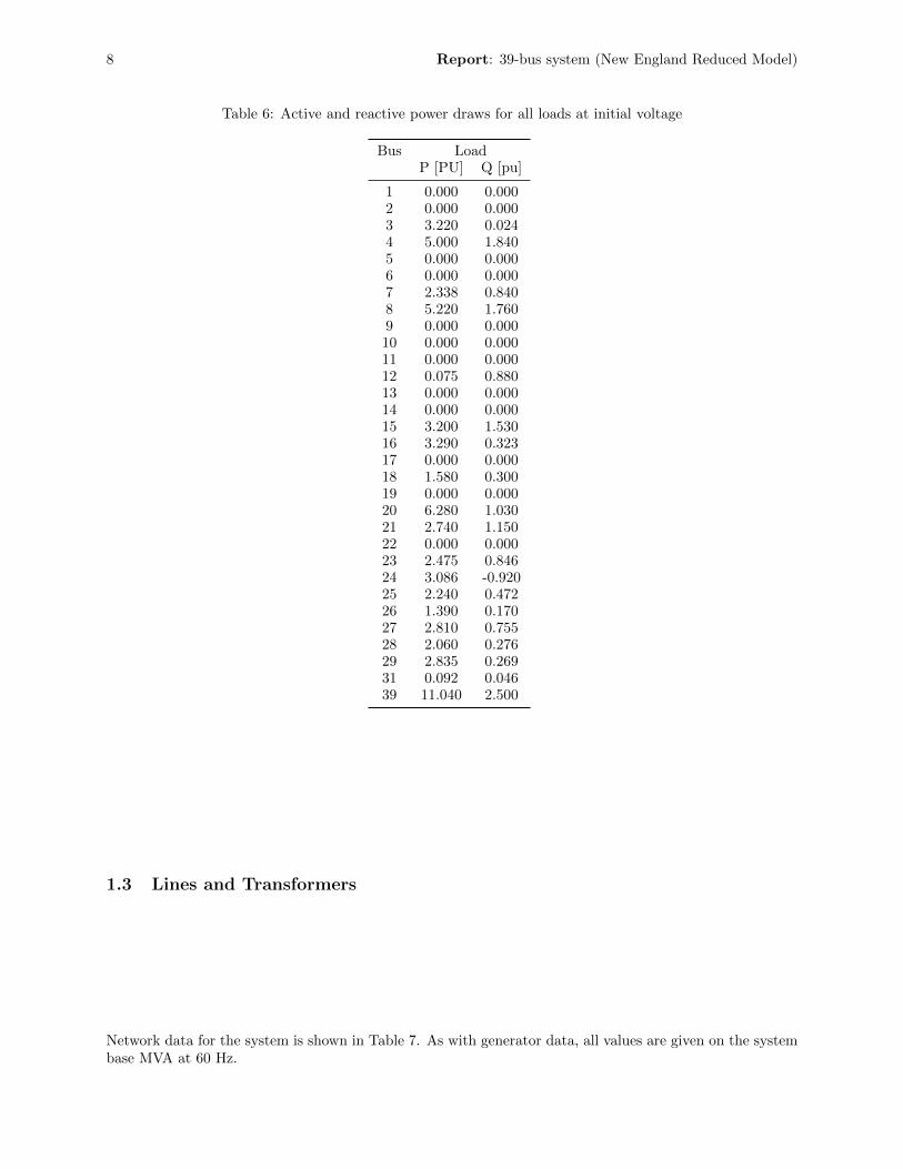
Table 6 contains load behavior at initial voltage. Due to the voltage dependence discussed above, thesevalues may not be accurate after voltages change.


Table 6: Active and reactive power draws for all loads at initial voltage

Bus LoadP [PU] Q [pu]

1 0.000 0.0002 0.000 0.0003 3.220 0.0244 5.000 1.8405 0.000 0.0006 0.000 0.0007 2.338 0.8408 5.220 1.7609 0.000 0.00010 0.000 0.00011 0.000 0.00012 0.075 0.88013 0.000 0.00014 0.000 0.00015 3.200 1.53016 3.290 0.32317 0.000 0.00018 1.580 0.30019 0.000 0.00020 6.280 1.03021 2.740 1.15022 0.000 0.00023 2.475 0.84624 3.086 -0.92025 2.240 0.47226 1.390 0.17027 2.810 0.75528 2.060 0.27629 2.835 0.26931 0.092 0.04639 11.040 2.500

1.3 Lines and Transformers

Network data for the system is shown in Table 7. As with generator data, all values are given on the systembase MVA at 60 Hz.


Table 7: Network data

Line Data Transformer Tap

From Bus To Bus R X B Magnitude Angle1 2 0.0035 0.0411 0.6987 - -1 39 0.001 0.025 0.75 - -2 3 0.0013 0.0151 0.2572 - -2 25 0.007 0.0086 0.146 - -3 4 0.0013 0.0213 0.2214 - -3 18 0.0011 0.0133 0.2138 - -4 5 0.0008 0.0128 0.1342 - -4 14 0.0008 0.0129 0.1382 - -5 6 0.0002 0.0026 0.0434 - -5 8 0.0008 0.0112 0.1476 - -6 7 0.0006 0.0092 0.113 - -6 11 0.0007 0.0082 0.1389 - -7 8 0.0004 0.0046 0.078 - -8 9 0.0023 0.0363 0.3804 - -9 39 0.001 0.025 1.2 - -10 11 0.0004 0.0043 0.0729 - -10 13 0.0004 0.0043 0.0729 - -13 14 0.0009 0.0101 0.1723 - -14 15 0.0018 0.0217 0.366 - -15 16 0.0009 0.0094 0.171 - -16 17 0.0007 0.0089 0.1342 - -16 19 0.0016 0.0195 0.304 - -16 21 0.0008 0.0135 0.2548 - -16 24 0.0003 0.0059 0.068 - -17 18 0.0007 0.0082 0.1319 - -17 27 0.0013 0.0173 0.3216 - -21 22 0.0008 0.014 0.2565 - -22 23 0.0006 0.0096 0.1846 - -23 24 0.0022 0.035 0.361 - -25 26 0.0032 0.0323 0.513 - -26 27 0.0014 0.0147 0.2396 - -26 28 0.0043 0.0474 0.7802 - -26 29 0.0057 0.0625 1.029 - -28 29 0.0014 0.0151 0.249 - -12 11 0.0016 0.0435 0 1.006 012 13 0.0016 0.0435 0 1.006 06 31 0 0.025 0 1.07 010 32 0 0.02 0 1.07 019 33 0.0007 0.0142 0 1.07 020 34 0.0009 0.018 0 1.009 022 35 0 0.0143 0 1.025 023 36 0.0005 0.0272 0 1 025 37 0.0006 0.0232 0 1.025 02 30 0 0.0181 0 1.025 029 38 0.0008 0.0156 0 1.025 019 20 0.0007 0.0138 0 1.06 0


1.4 Power and Voltage Setpoints

Table 8 contains power and voltage setpoint data, specified on the system MVA base. Note that Generator2 is the swing node, and Generator 1 represents the aggregation of a large number of generators.

Table 8: Power and voltage setpoint data

Bus Type Voltage Load Generator

[PU] MW MVar MW MVar Unit No.1 PQ - 0 0 0 02 PQ - 0 0 0 03 PQ - 322 2.4 0 04 PQ - 500 184 0 05 PQ - 0 0 0 06 PQ - 0 0 0 07 PQ - 233.8 84 0 08 PQ - 522 176 0 09 PQ - 0 0 0 010 PQ - 0 0 0 011 PQ - 0 0 0 012 PQ - 7.5 88 0 013 PQ - 0 0 0 014 PQ - 0 0 0 015 PQ - 320 153 0 016 PQ - 329 32.3 0 017 PQ - 0 0 0 018 PQ - 158 30 0 019 PQ - 0 0 0 020 PQ - 628 103 0 021 PQ - 274 115 0 022 PQ - 0 0 0 023 PQ - 247.5 84.6 0 024 PQ - 308.6 -92 0 025 PQ - 224 47.2 0 026 PQ - 139 17 0 027 PQ - 281 75.5 0 028 PQ - 206 27.6 0 029 PQ - 283.5 26.9 0 030 PV 1.0475 0 0 250 - Gen1031 PV 0.982 9.2 4.6 - - Gen232 PV 0.9831 0 0 650 - Gen333 PV 0.9972 0 0 632 - Gen434 PV 1.0123 0 0 508 - Gen535 PV 1.0493 0 0 650 - Gen636 PV 1.0635 0 0 560 - Gen737 PV 1.0278 0 0 540 - Gen838 PV 1.0265 0 0 830 - Gen939 PV 1.03 1104 250 1000 - Gen1

This completes the description of the system and its model. The remainder of this report focuses onthe three analyses performed on the system: load flow, small signal stability assessment via Eigenvaluecalculation, and numerical simulation. The results of load flow analysis are presented in the next section.


2 Load Flow Results

Load flow for the system was calculated using MATLAB. The results are in Table 9. Note that all voltages,active power values, and reactive power values are given in per unit on the system MVA base.

For a more complete description of power flow, including flow on each line, see Section 5.2 in the Appendix.

Table 9: Power flow results

Bus V Angle [deg] Bus Total Load Generator

P Q P Q P Q Unit No.1 1.0474 -8.44 0 0 0 02 1.0487 -5.75 0 0 0 03 1.0302 -8.6 -322 -2.4 -322 -2.44 1.0039 -9.61 -500 -184 -500 -1845 1.0053 -8.61 0 0 0 06 1.0077 -7.95 0 0 0 07 0.997 -10.12 -233.8 -84 -233.8 -848 0.996 -10.62 -522 -176 -522 -1769 1.0282 -10.32 0 0 0 010 1.0172 -5.43 0 0 0 011 1.0127 -6.28 0 0 0 012 1.0002 -6.24 -7.5 -88 -7.5 -8813 1.0143 -6.1 0 0 0 014 1.0117 -7.66 0 0 0 015 1.0154 -7.74 -320 -153 -320 -15316 1.0318 -6.19 -329 -32.3 -329 -32.317 1.0336 -7.3 0 0 0 018 1.0309 -8.22 -158 -30 -158 -3019 1.0499 -1.02 0 0 0 020 0.9912 -2.01 -628 -103 -628 -10321 1.0318 -3.78 -274 -115 -274 -11522 1.0498 0.67 0 0 0 023 1.0448 0.47 -247.5 -84.6 -247.5 -84.624 1.0373 -6.07 -308.6 92.2 -308.6 92.225 1.0576 -4.36 -224 -47.2 -224 -47.226 1.0521 -5.53 -139 -17 -139 -1727 1.0377 -7.5 -281 -75.5 -281 -75.528 1.0501 -2.01 -206 -27.6 -206 -27.629 1.0499 0.74 -283.5 -26.9 -283.5 -26.930 1.0475 -3.33 250 146.16 250 146.16 1031 0.982 0 511.61 193.65 -9.2 -4.6 520.81 198.25 232 0.9831 2.57 650 205.14 650 205.14 333 0.9972 4.19 632 109.91 632 109.91 434 1.0123 3.17 508 165.76 508 165.76 535 1.0493 5.63 650 212.41 650 212.41 636 1.0635 8.32 560 101.17 560 101.17 737 1.0278 2.42 540 0.44 540 0.44 838 1.0265 7.81 830 22.84 830 22.84 939 1.03 -10.05 -104 -161.7 -1104 -250 1000 88.28 1


3 Small Disturbance Analysis

Small signal stability was assessed by calculating Eigenvalues of the system. To find Eigenvalues, we firstcalculated reduced A matrices as follows:

x = f(x, y)Differential eq.

| 0 = g(x, y)Algebraic eq.

Linearize: ∆x = fx∆x+ fy∆y | 0 = gx∆x+ gy∆y

Eliminate algebraic equations: ∆x = (fx − fyg−1y gx)

Reduced A matrices

∆x

Eigenvalues, which correspond to machine oscillatory modes, are calculated from the reduced A matrices.Some Eigenvalues of our system are given in Table 10 below. To access all Eigenvalues calculated in ouranalysis, see Section 5.1 in the Appendix.

Table 10: Eigenvalues calculated through small disturbance analysis

Index Real part Imaginary part

27 -2.553 j10.56629 -1.8494 j10.02831 -1.5817 j8.550333 -2.5633 j8.670635 -1.8626 j7.438837 -1.3118 j7.108139 -1.8437 j7.081241 -1.523 j6.318057 -2.9563 j2.5076

The Eigenvalues in Table 10 are plotted in Figure 4.

−3.5 −3 −2.5 −2 −1.5 −12

3

4

5

6

7

8

9

10

11

12

27

29

3133

353739

41

57

Real Axis

Imag

inar

y A

xis

Student Version of MATLAB

Figure 4: Graphical depiction of Eigenvalues


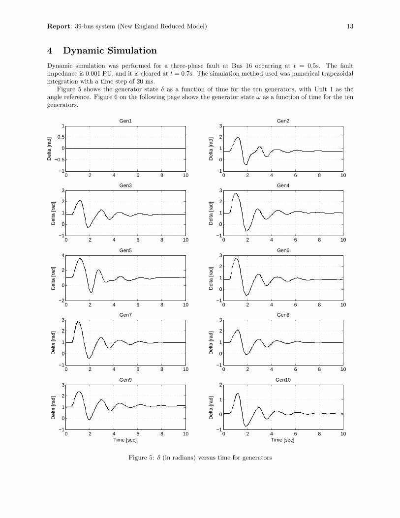
4 Dynamic Simulation

Dynamic simulation was performed for a three-phase fault at Bus 16 occurring at t = 0.5s. The faultimpedance is 0.001 PU, and it is cleared at t = 0.7s. The simulation method used was numerical trapezoidalintegration with a time step of 20 ms.

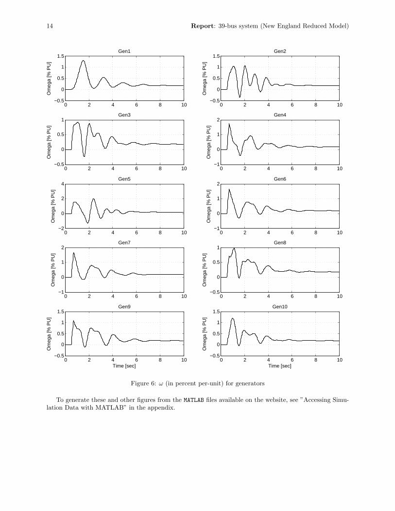
Figure 5 shows the generator state δ as a function of time for the ten generators, with Unit 1 as theangle reference. Figure 6 on the following page shows the generator state ω as a function of time for the tengenerators.

0 2 4 6 8 10−1

−0.5

0

0.5

1Gen1

Del

ta [r

ad]

0 2 4 6 8 10−1

0

1

2

3Gen2

Del

ta [r

ad]

0 2 4 6 8 10−1

0

1

2

3Gen3

Del

ta [r

ad]

0 2 4 6 8 10−1

0

1

2

3Gen4

Del

ta [r

ad]

0 2 4 6 8 10−2

0

2

4Gen5

Del

ta [r

ad]

0 2 4 6 8 10−1

0

1

2

3Gen6

Del

ta [r

ad]

0 2 4 6 8 10−1

0

1

2

3Gen7

Del

ta [r

ad]

0 2 4 6 8 10−1

0

1

2

3Gen8

Del

ta [r

ad]

0 2 4 6 8 10−1

0

1

2

3Gen9

Time [sec]

Del

ta [r

ad]

0 2 4 6 8 10−1

0

1

2Gen10

Time [sec]

Del

ta [r

ad]


Figure 5: δ (in radians) versus time for generators


0 2 4 6 8 10−0.5

0

0.5

1

1.5Gen1

Om

ega

[% P

U]

0 2 4 6 8 10−0.5

0

0.5

1

1.5Gen2

Om

ega

[% P

U]

0 2 4 6 8 10−0.5

0

0.5

1Gen3

Om

ega

[% P

U]

0 2 4 6 8 10−1

0

1

2Gen4

Om

ega

[% P

U]

0 2 4 6 8 10−2

0

2

4Gen5

Om

ega

[% P

U]

0 2 4 6 8 10−1

0

1

2Gen6

Om

ega

[% P

U]

0 2 4 6 8 10−1

0

1

2Gen7

Om

ega

[% P

U]

0 2 4 6 8 10−0.5

0

0.5

1Gen8

Om

ega

[% P

U]

0 2 4 6 8 10−0.5

0

0.5

1

1.5Gen9

Time [sec]

Om

ega

[% P

U]

0 2 4 6 8 10−0.5

0

0.5

1

1.5Gen10

Time [sec]

Om

ega

[% P

U]


Figure 6: ω (in percent per-unit) for generators

To generate these and other figures from the MATLAB files available on the website, see ”Accessing Simu-lation Data with MATLAB” in the appendix.


5 Appendix

5.1 Accessing Simulation Data with MATLAB R©

There are seven MATLAB R©.mat files available for download. Each .mat file has a csv counterpart forthose who prefer to work with Excel or another CSV-friendly program (the procedure described here maybe adapted for such programs). Each file is described below.

• time.mat is a row vector with 677 elements. This vector represents the simulation time period withincrements of 20ms. To observe the variation of any model variable with respect to time, simply plotthe corresponding row of x.mat or y.mat versus time.mat.

• x.mat contains 209 row vectors, each corresponding to a model state variable. See Table 11.

• x0.mat contains 209 elements corresponding to initial values of model state variables. It is indexed thesame as x.mat.

• y.mat contains 617 row vectors, each corresponding to a non-state variable in the model. See Table11.

• y0.mat contains 617 elements corresponding to initial values of non-state variables. It is indexed thesame as y.mat.

• Aeig.mat contains 209 complex elements corresponding to system Eigenvalues. To obtain any entryof Table 10, one need only extract the element of Aeig corresponding to that entry’s Index. Of course,there are many more Eigenvalues stored in Aeig than those listed in Table 10, and all Eigenvalues maybe easily plotted so long as care is taken in isolating the real and imaginary parts.

• Ared.mat is a 209-by-209 variable containing reduced A matrix data for the system. (Reduced Amatrices are discussed in Section 3.)

Model state variables are stored in x.mat while non-state variables are located in y.mat. Table 11maps from these files to specific model variables by specifying the range of variables corresponding to eachcomponent of the model. The order of variables within a component’s range is discussed in the next fivesubsections.

Table 11: Mapping from MATLAB R©files to simulation data

Model Model ID x range y range Descriptionfrom to from to

Generator G1 1 4 1 13 4 x states and 13 y variablesG10 37 49 118 130

AVR G1 110 114 438 448 5 x states and 11 y variablesG10 155 159 537 547

PSS G1 160 164 548 554 5 x states and 7 y variablesG10 205 209 611 617

Load Bus1 47 48 303 306 2 x states and 4 y variablesBus39 107 108 423 426 (x states are real and reactive power)

Network Bus1 131 134 4 y variablesBus39 283 286

5.1.1 Variable Indexing

This section defines all variables contained in the MATLAB files. When writing code to extract specific variables,refer to this section to determine which indices to use.


Generator Variables (See Section 1.1.1)

x1 : E′qx2 : E′dx3 : δx4 : ω

y1 : Vry2 : Viy3 : Iry4 : Iiy5 : Vdy6 : Vqy7 : Idy8 : Iqy9 : ψdy10 : ψqy11 : Efdy12 : ωy13 : Tmech

AVR Variables (See Section 1.1.3)

x1 : Vfx2 : Efdx3 : xix4 : VREF

y1 : Vry2 : Viy3 : VTy4 : VPSSy5 : xerry6 : xtgry7 : Efdy8 : Upper Limit Detectory9 : Lower Limit Detectory10 : Upper Limit Switchy11 : Lower Limit Switch

PSS Variables (See Section 1.1.5)

x1 : xWx2 : xPx3 : xQ

y1 : ω (input)y2 : VWy3 : VPy4 : Vouty5 : VPSSy6 : VPSS,Max − Vouty7 : Vout − VPSS,Min

Load Variables (See Section 1.2.1)

x1 : Px2 : Q

y1 : Vry2 : Viy3 : Iry4 : Ii

Network Variables (See ??) Network variables are indexed in the MATLAB files as follows:

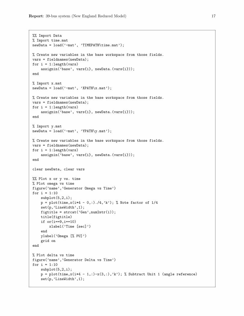
5.1.2 Example Application

The code below will generate Figures 5 and 6. By modifying or adapting this code, the reader may plot ormanipulate any variables in x.mat and y.mat.

(Note: The placeholders ”TIMEPATH”, ”XPATH”, and ”YPATH” should be replaced with paths to therespective files on your computer.)


%% Import Data

% Import time.mat

newData = load(’-mat’, ’TIMEPATH\time.mat’);

% Create new variables in the base workspace from those fields.

vars = fieldnames(newData);

for i = 1:length(vars)

assignin(’base’, vars{i}, newData.(vars{i}));

end

% Import x.mat

newData = load(’-mat’, ’XPATH\x.mat’);





end

% Import y.mat

newData = load(’-mat’, ’YPATH\y.mat’);





end

clear newData, clear vars

%% Plot x or y vs. time

% Plot omega vs time

figure(’name’,’Generator Omega vs Time’)

for i = 1:10

subplot(5,2,i);

p = plot(time,x(i*4 - 0,:)./4,’k’); % Note factor of 1/4

set(p,’LineWidth’,1);

figtitle = strcat(’Gen’,num2str(i));

title(figtitle)

if or(i==9,i==10)

xlabel(’Time [sec]’)

end

ylabel(’Omega [% PU]’)

grid on

end

% Plot delta vs time

figure(’name’,’Generator Delta vs Time’)

for i = 1:10

subplot(5,2,i);

p = plot(time,x(i*4 - 1,:)-x(3,:),’k’); % Subtract Unit 1 (angle reference)

set(p,’LineWidth’,1);


figtitle = strcat(’Gen’,num2str(i));

title(figtitle)

if or(i==9,i==10)

xlabel(’Time [sec]’)

end

ylabel(’Delta [rad]’)

grid on

end

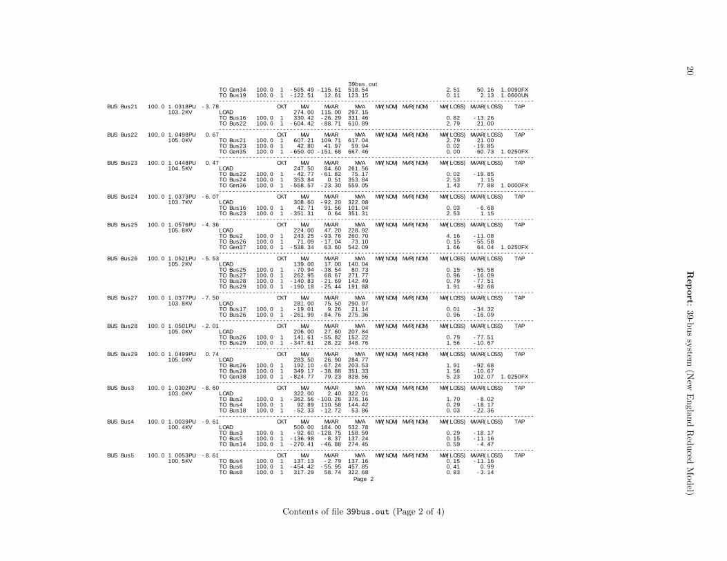
5.2 Contents of file 39bus.out

The next four pages show the contents of the file 39bus.out. This file contains power flow data with enoughgranularity to observe flows on all lines.

Report:

39-b

us

system

(New

En

gland

Red

uced

Mod

el)19

39bus.out IEEE 39 bus test system

BUS Bus1 100.0 1.0474PU -8.44 CKT MW MVAR MVA MW(NOM) MVR(NOM) MW(LOSS) MVAR(LOSS) TAP 104.7KV TO Bus2 100.0 1 -124.34 -28.32 127.52 0.50 -70.92 TO Gen39 100.0 1 124.34 28.32 127.52 0.18 -76.30 --------------------------------------------------------------------------------------------- BUS Bus10 100.0 1.0172PU -5.43 CKT MW MVAR MVA MW(NOM) MVR(NOM) MW(LOSS) MVAR(LOSS) TAP 101.7KV TO Bus11 100.0 1 365.25 70.36 371.96 0.54 -1.74 TO Bus13 100.0 1 284.75 38.65 287.37 0.32 -4.07 TO Gen32 100.0 1 -650.00 -109.01 659.08 0.00 96.14 1.0700FX --------------------------------------------------------------------------------------------- BUS Bus11 100.0 1.0127PU -6.28 CKT MW MVAR MVA MW(NOM) MVR(NOM) MW(LOSS) MVAR(LOSS) TAP 101.3KV TO Bus6 100.0 1 364.76 29.01 365.92 0.92 -3.43 TO Bus10 100.0 1 -364.71 -72.10 371.77 0.54 -1.74 TO Bus12 100.0 1 -0.06 43.09 43.09 0.03 0.79 1.0060UN --------------------------------------------------------------------------------------------- BUS Bus12 100.0 1.0002PU -6.24 CKT MW MVAR MVA MW(NOM) MVR(NOM) MW(LOSS) MVAR(LOSS) TAP 100.0KV LOAD 7.50 88.00 88.32 TO Bus11 100.0 1 0.09 -42.30 42.30 0.03 0.79 1.0060FX TO Bus13 100.0 1 -7.59 -45.70 46.32 0.03 0.94 1.0060FX --------------------------------------------------------------------------------------------- BUS Bus13 100.0 1.0143PU -6.10 CKT MW MVAR MVA MW(NOM) MVR(NOM) MW(LOSS) MVAR(LOSS) TAP 101.4KV TO Bus10 100.0 1 -284.43 -42.72 287.62 0.32 -4.07 TO Bus14 100.0 1 276.81 -3.92 276.84 0.67 -10.16 TO Bus12 100.0 1 7.62 46.64 47.26 0.03 0.94 1.0060UN --------------------------------------------------------------------------------------------- BUS Bus14 100.0 1.0117PU -7.66 CKT MW MVAR MVA MW(NOM) MVR(NOM) MW(LOSS) MVAR(LOSS) TAP 101.2KV TO Bus4 100.0 1 271.01 42.41 274.31 0.59 -4.47 TO Bus13 100.0 1 -276.14 -6.23 276.21 0.67 -10.16 TO Bus15 100.0 1 5.14 -36.17 36.54 0.01 -37.53 --------------------------------------------------------------------------------------------- BUS Bus15 100.0 1.0154PU -7.74 CKT MW MVAR MVA MW(NOM) MVR(NOM) MW(LOSS) MVAR(LOSS) TAP 101.5KV LOAD 320.00 153.00 354.70 TO Bus14 100.0 1 -5.13 -1.36 5.31 0.01 -37.53 TO Bus16 100.0 1 -314.87 -151.64 349.48 1.04 -7.02 --------------------------------------------------------------------------------------------- BUS Bus16 100.0 1.0318PU -6.19 CKT MW MVAR MVA MW(NOM) MVR(NOM) MW(LOSS) MVAR(LOSS) TAP 103.2KV LOAD 329.00 32.30 330.58 TO Bus15 100.0 1 315.91 144.63 347.45 1.04 -7.02 TO Bus17 100.0 1 230.04 -43.63 234.14 0.36 -9.78 TO Bus19 100.0 1 -502.68 -48.08 504.97 3.81 13.54 TO Bus21 100.0 1 -329.60 13.03 329.85 0.82 -13.26 TO Bus24 100.0 1 -42.68 -98.24 107.11 0.03 -6.68 --------------------------------------------------------------------------------------------- BUS Bus17 100.0 1.0336PU -7.30 CKT MW MVAR MVA MW(NOM) MVR(NOM) MW(LOSS) MVAR(LOSS) TAP 103.4KV TO Bus16 100.0 1 -229.68 33.85 232.16 0.36 -9.78 TO Bus18 100.0 1 210.66 9.73 210.88 0.29 -10.63 TO Bus27 100.0 1 19.02 -43.58 47.55 0.01 -34.32 --------------------------------------------------------------------------------------------- BUS Bus18 100.0 1.0309PU -8.22 CKT MW MVAR MVA MW(NOM) MVR(NOM) MW(LOSS) MVAR(LOSS) TAP 103.1KV LOAD 158.00 30.00 160.82 TO Bus3 100.0 1 52.36 -9.64 53.24 0.03 -22.36 TO Bus17 100.0 1 -210.36 -20.36 211.35 0.29 -10.63 --------------------------------------------------------------------------------------------- BUS Bus19 100.0 1.0499PU -1.02 CKT MW MVAR MVA MW(NOM) MVR(NOM) MW(LOSS) MVAR(LOSS) TAP 105.0KV TO Bus16 100.0 1 506.49 61.62 510.22 3.81 13.54 TO Gen33 100.0 1 -629.10 -51.14 631.18 2.90 58.76 1.0700FX TO Bus20 100.0 1 122.62 -10.48 123.06 0.11 2.13 1.0600FX --------------------------------------------------------------------------------------------- BUS Bus2 100.0 1.0487PU -5.75 CKT MW MVAR MVA MW(NOM) MVR(NOM) MW(LOSS) MVAR(LOSS) TAP 104.9KV TO Bus1 100.0 1 124.83 -42.60 131.90 0.50 -70.92 TO Bus3 100.0 1 364.26 92.24 375.76 1.70 -8.02 TO Bus25 100.0 1 -239.09 82.68 252.98 4.16 -11.08 TO Gen30 100.0 1 -250.00 -132.32 282.86 0.00 13.83 1.0250FX --------------------------------------------------------------------------------------------- BUS Bus20 100.0 0.9912PU -2.01 CKT MW MVAR MVA MW(NOM) MVR(NOM) MW(LOSS) MVAR(LOSS) TAP 99.1KV LOAD 628.00 103.00 636.39

Page 1

Figure 7: Contents of file 39bus.out (Page 1 of 4)

20

Report:

39-bu

ssy

stem(N

ewE

nglan

dR

edu

cedM

od

el)

39bus.out TO Gen34 100.0 1 -505.49 -115.61 518.54 2.51 50.16 1.0090FX TO Bus19 100.0 1 -122.51 12.61 123.15 0.11 2.13 1.0600UN --------------------------------------------------------------------------------------------- BUS Bus21 100.0 1.0318PU -3.78 CKT MW MVAR MVA MW(NOM) MVR(NOM) MW(LOSS) MVAR(LOSS) TAP 103.2KV LOAD 274.00 115.00 297.15 TO Bus16 100.0 1 330.42 -26.29 331.46 0.82 -13.26 TO Bus22 100.0 1 -604.42 -88.71 610.89 2.79 21.00 --------------------------------------------------------------------------------------------- BUS Bus22 100.0 1.0498PU 0.67 CKT MW MVAR MVA MW(NOM) MVR(NOM) MW(LOSS) MVAR(LOSS) TAP 105.0KV TO Bus21 100.0 1 607.21 109.71 617.04 2.79 21.00 TO Bus23 100.0 1 42.80 41.97 59.94 0.02 -19.85 TO Gen35 100.0 1 -650.00 -151.68 667.46 0.00 60.73 1.0250FX --------------------------------------------------------------------------------------------- BUS Bus23 100.0 1.0448PU 0.47 CKT MW MVAR MVA MW(NOM) MVR(NOM) MW(LOSS) MVAR(LOSS) TAP 104.5KV LOAD 247.50 84.60 261.56 TO Bus22 100.0 1 -42.77 -61.82 75.17 0.02 -19.85 TO Bus24 100.0 1 353.84 0.51 353.84 2.53 1.15 TO Gen36 100.0 1 -558.57 -23.30 559.05 1.43 77.88 1.0000FX --------------------------------------------------------------------------------------------- BUS Bus24 100.0 1.0373PU -6.07 CKT MW MVAR MVA MW(NOM) MVR(NOM) MW(LOSS) MVAR(LOSS) TAP 103.7KV LOAD 308.60 -92.20 322.08 TO Bus16 100.0 1 42.71 91.56 101.04 0.03 -6.68 TO Bus23 100.0 1 -351.31 0.64 351.31 2.53 1.15 --------------------------------------------------------------------------------------------- BUS Bus25 100.0 1.0576PU -4.36 CKT MW MVAR MVA MW(NOM) MVR(NOM) MW(LOSS) MVAR(LOSS) TAP 105.8KV LOAD 224.00 47.20 228.92 TO Bus2 100.0 1 243.25 -93.76 260.70 4.16 -11.08 TO Bus26 100.0 1 71.09 -17.04 73.10 0.15 -55.58 TO Gen37 100.0 1 -538.34 63.60 542.09 1.66 64.04 1.0250FX --------------------------------------------------------------------------------------------- BUS Bus26 100.0 1.0521PU -5.53 CKT MW MVAR MVA MW(NOM) MVR(NOM) MW(LOSS) MVAR(LOSS) TAP 105.2KV LOAD 139.00 17.00 140.04 TO Bus25 100.0 1 -70.94 -38.54 80.73 0.15 -55.58 TO Bus27 100.0 1 262.95 68.67 271.77 0.96 -16.09 TO Bus28 100.0 1 -140.83 -21.69 142.49 0.79 -77.51 TO Bus29 100.0 1 -190.18 -25.44 191.88 1.91 -92.68 --------------------------------------------------------------------------------------------- BUS Bus27 100.0 1.0377PU -7.50 CKT MW MVAR MVA MW(NOM) MVR(NOM) MW(LOSS) MVAR(LOSS) TAP 103.8KV LOAD 281.00 75.50 290.97 TO Bus17 100.0 1 -19.01 9.26 21.14 0.01 -34.32 TO Bus26 100.0 1 -261.99 -84.76 275.36 0.96 -16.09 --------------------------------------------------------------------------------------------- BUS Bus28 100.0 1.0501PU -2.01 CKT MW MVAR MVA MW(NOM) MVR(NOM) MW(LOSS) MVAR(LOSS) TAP 105.0KV LOAD 206.00 27.60 207.84 TO Bus26 100.0 1 141.61 -55.82 152.22 0.79 -77.51 TO Bus29 100.0 1 -347.61 28.22 348.76 1.56 -10.67 --------------------------------------------------------------------------------------------- BUS Bus29 100.0 1.0499PU 0.74 CKT MW MVAR MVA MW(NOM) MVR(NOM) MW(LOSS) MVAR(LOSS) TAP 105.0KV LOAD 283.50 26.90 284.77 TO Bus26 100.0 1 192.10 -67.24 203.53 1.91 -92.68 TO Bus28 100.0 1 349.17 -38.88 351.33 1.56 -10.67 TO Gen38 100.0 1 -824.77 79.23 828.56 5.23 102.07 1.0250FX --------------------------------------------------------------------------------------------- BUS Bus3 100.0 1.0302PU -8.60 CKT MW MVAR MVA MW(NOM) MVR(NOM) MW(LOSS) MVAR(LOSS) TAP 103.0KV LOAD 322.00 2.40 322.01 TO Bus2 100.0 1 -362.56 -100.26 376.16 1.70 -8.02 TO Bus4 100.0 1 92.89 110.58 144.42 0.29 -18.17 TO Bus18 100.0 1 -52.33 -12.72 53.86 0.03 -22.36 --------------------------------------------------------------------------------------------- BUS Bus4 100.0 1.0039PU -9.61 CKT MW MVAR MVA MW(NOM) MVR(NOM) MW(LOSS) MVAR(LOSS) TAP 100.4KV LOAD 500.00 184.00 532.78 TO Bus3 100.0 1 -92.60 -128.75 158.59 0.29 -18.17 TO Bus5 100.0 1 -136.98 -8.37 137.24 0.15 -11.16 TO Bus14 100.0 1 -270.41 -46.88 274.45 0.59 -4.47 --------------------------------------------------------------------------------------------- BUS Bus5 100.0 1.0053PU -8.61 CKT MW MVAR MVA MW(NOM) MVR(NOM) MW(LOSS) MVAR(LOSS) TAP 100.5KV TO Bus4 100.0 1 137.13 -2.79 137.16 0.15 -11.16 TO Bus6 100.0 1 -454.42 -55.95 457.85 0.41 0.99 TO Bus8 100.0 1 317.29 58.74 322.68 0.83 -3.14

Page 2

Contents of file 39bus.out (Page 2 of 4)

Report:

39-b

us

system

(New

En

gland

Red

uced

Mod

el)21

39bus.out --------------------------------------------------------------------------------------------- BUS Bus6 100.0 1.0077PU -7.95 CKT MW MVAR MVA MW(NOM) MVR(NOM) MW(LOSS) MVAR(LOSS) TAP 100.8KV TO Bus5 100.0 1 454.84 56.94 458.39 0.41 0.99 TO Bus7 100.0 1 420.62 91.57 430.47 1.10 5.53 TO Bus11 100.0 1 -363.85 -32.44 365.29 0.92 -3.43 TO Gen31 100.0 1 -511.61 -116.07 524.61 0.00 77.58 1.0700FX --------------------------------------------------------------------------------------------- BUS Bus7 100.0 0.9970PU -10.12 CKT MW MVAR MVA MW(NOM) MVR(NOM) MW(LOSS) MVAR(LOSS) TAP 99.7KV LOAD 233.80 84.00 248.43 TO Bus6 100.0 1 -419.52 -86.04 428.25 1.10 5.53 TO Bus8 100.0 1 185.72 2.04 185.73 0.14 -6.15 --------------------------------------------------------------------------------------------- BUS Bus8 100.0 0.9960PU -10.62 CKT MW MVAR MVA MW(NOM) MVR(NOM) MW(LOSS) MVAR(LOSS) TAP 99.6KV LOAD 522.00 176.00 550.87 TO Bus5 100.0 1 -316.46 -61.88 322.45 0.83 -3.14 TO Bus7 100.0 1 -185.58 -8.19 185.76 0.14 -6.15 TO Bus9 100.0 1 -19.96 -105.94 107.80 0.18 -36.06 --------------------------------------------------------------------------------------------- BUS Bus9 100.0 1.0282PU -10.32 CKT MW MVAR MVA MW(NOM) MVR(NOM) MW(LOSS) MVAR(LOSS) TAP 102.8KV TO Bus8 100.0 1 20.15 69.88 72.73 0.18 -36.06 TO Gen39 100.0 1 -20.15 -69.88 72.73 0.00 -126.98 --------------------------------------------------------------------------------------------- BUS Gen30 100.0 1.0475PU -3.33 CKT MW MVAR MVA MW(NOM) MVR(NOM) MW(LOSS) MVAR(LOSS) TAP 104.8KV GENERATION 250.00 146.16 289.59 ( 250.00 0.00) TO Bus2 100.0 1 250.00 146.16 289.59 0.00 13.83 1.0250UN --------------------------------------------------------------------------------------------- BUS Gen31 100.0 0.9820PU 0.00 CKT MW MVAR MVA MW(NOM) MVR(NOM) MW(LOSS) MVAR(LOSS) TAP 98.2KV LOAD 9.20 4.60 10.29 GENERATION 520.81 198.25 557.27 ( 0.00 0.00) TO Bus6 100.0 1 511.61 193.65 547.03 0.00 77.58 1.0700UN --------------------------------------------------------------------------------------------- BUS Gen32 100.0 0.9831PU 2.57 CKT MW MVAR MVA MW(NOM) MVR(NOM) MW(LOSS) MVAR(LOSS) TAP 98.3KV GENERATION 650.00 205.15 681.60 ( 650.00 0.00) TO Bus10 100.0 1 650.00 205.15 681.60 0.00 96.14 1.0700UN --------------------------------------------------------------------------------------------- BUS Gen33 100.0 0.9972PU 4.19 CKT MW MVAR MVA MW(NOM) MVR(NOM) MW(LOSS) MVAR(LOSS) TAP 99.7KV GENERATION 632.00 109.91 641.49 ( 632.00 0.00) TO Bus19 100.0 1 632.00 109.91 641.49 2.90 58.76 1.0700UN --------------------------------------------------------------------------------------------- BUS Gen34 100.0 1.0123PU 3.18 CKT MW MVAR MVA MW(NOM) MVR(NOM) MW(LOSS) MVAR(LOSS) TAP 101.2KV GENERATION 508.00 165.76 534.36 ( 508.00 0.00) TO Bus20 100.0 1 508.00 165.76 534.36 2.51 50.16 1.0090UN --------------------------------------------------------------------------------------------- BUS Gen35 100.0 1.0493PU 5.63 CKT MW MVAR MVA MW(NOM) MVR(NOM) MW(LOSS) MVAR(LOSS) TAP 104.9KV GENERATION 650.00 212.41 683.83 ( 650.00 0.00) TO Bus22 100.0 1 650.00 212.41 683.83 0.00 60.73 1.0250UN --------------------------------------------------------------------------------------------- BUS Gen36 100.0 1.0635PU 8.32 CKT MW MVAR MVA MW(NOM) MVR(NOM) MW(LOSS) MVAR(LOSS) TAP 106.4KV GENERATION 560.00 101.17 569.07 ( 560.00 0.00) TO Bus23 100.0 1 560.00 101.17 569.07 1.43 77.88 1.0000UN --------------------------------------------------------------------------------------------- BUS Gen37 100.0 1.0278PU 2.42 CKT MW MVAR MVA MW(NOM) MVR(NOM) MW(LOSS) MVAR(LOSS) TAP 102.8KV GENERATION 540.00 0.44 540.00 ( 540.00 0.00) TO Bus25 100.0 1 540.00 0.44 540.00 1.66 64.04 1.0250UN --------------------------------------------------------------------------------------------- BUS Gen38 100.0 1.0265PU 7.81 CKT MW MVAR MVA MW(NOM) MVR(NOM) MW(LOSS) MVAR(LOSS) TAP 102.6KV GENERATION 830.00 22.84 830.31 ( 830.00 0.00) TO Bus29 100.0 1 830.00 22.84 830.31 5.23 102.07 1.0250UN --------------------------------------------------------------------------------------------- BUS Gen39 100.0 1.0300PU -10.05 CKT MW MVAR MVA MW(NOM) MVR(NOM) MW(LOSS) MVAR(LOSS) TAP 103.0KV LOAD 1104.00 250.00 1131.95 GENERATION 1000.00 88.28 1003.89 (1000.00 0.00) TO Bus1 100.0 1 -124.15 -104.61 162.35 0.18 -76.30 TO Bus9 100.0 1 20.15 -57.10 60.56 0.00 -126.98 ---------------------------------------------------------------------------------------------

SYSTEM TOTALS ------ ------

Page 3


22

Report:

39-bu

ssy

stem(N

ewE

nglan

dR

edu

cedM

od

el)

39bus.out MW MVAR GENERATION 6140.81 1250.37 LOAD 6097.10 1408.90 LOSSES 43.71 -158.52 BUS SHUNTS 0.00 0.00 LINE SHUNTS 0.00 0.00 SWITCHED SHUNTS 0.00

MISMATCH 0.00 0.01

BASE MVA : 100.0 TOLERANCE: 0.000100 PU

SLACK BUSES ----- ----- Gen31 100.0

Page 4



References

[1] T. Athay, R. Podmore, and S. Virmani. “A Practical Method for the Direct Analysis of TransientStability”. In: IEEE Transactions on Power Apparatus and Systems PAS-98 (2 Mar. 1979), pp. 573–584.

[2] M. A. Pai. Energy function analysis for power system stability. The Kluwer international series inengineering and computer science. Power electronics and power systems. Boston: Kluwer AcademicPublishers, 1989.

[3] Peter W Sauer and M. A Pai. Power system dynamics and stability. English. Champaign, IL.: StipesPublishing L.L.C., 2006.

ieee pes task force on benchmark systems for stability ... · ieee pes task force on benchmark...

Documents