ieee sensors journal, vol. 16, no. 12, june 15, 2016 …jasonku/pdf/lighting_ieee2016.pdfieee...

IEEE SENSORS JOURNAL, VOL. 16, NO. 12, JUNE 15, 2016 4981

Urban Street Lighting Infrastructure MonitoringUsing a Mobile Sensor Platform

Sumeet Kumar, Ajay Deshpande, Stephen S. Ho, Jason S. Ku, and Sanjay E. Sarma

Abstract— We present a system for collecting and analyzinginformation on street lighting infrastructure. We develop a car-mounted sensor platform that enables collection and logging ofdata on street lights during night-time drive-bys. We addressseveral signal processing problems that are key to mappingstreet illumination levels, identifying street lamps, estimatingtheir heights, and geotagging them. Specifically, we highlight animage recognition algorithm to identify street lamps from thevideo data collected by the sensor platform and its subsequentuse in estimating the heights of street lamps. We also outline aframework to improve vehicle location estimates by combiningsensor observations in an extended Kalman filter framework. Oureventual goal is to develop a semi-live virtual 3-D street lightingmodel at urban scale that enables citizens and decision makersto assess and optimize performance of nighttime street lighting.

Index Terms— Sensors, urban sensing, mobile sensing,machine vision, image recognition, machine learning, geotagging,automation.

I. INTRODUCTION

THERE are nearly 40 million street lights in the USalone, and they consume 31 TWh of energy annually [1].

Worldwide numbers will increase with urbanization as billionsof people move to urban centers. International lightingstandards require a certain threshold of street lighting rangingfrom 1 lux of light at the surface of residential suburbs to50 lux at road intersections [2], [3]. Oddly, the science ofstreetlight placement is relatively primitive today, and themeans to monitor how much light reaches the street are verylimited. The standards for measuring lighting are complicated,manual, and rarely implemented at a city-wide scale.

Furthermore, like much of the infrastructure in thedeveloped word, lighting infrastructure has aged. Monitoringstreetlights is a tedious manual task that relies on inspectionand incident reports. Matters are not helped by the2008 financial crisis, after which many cities have faced

Manuscript received February 1, 2016; revised March 22, 2016; acceptedMarch 29, 2016. Date of publication April 8, 2016; date of current versionMay 17, 2016. This work was supported by Ferrovial Servicios. The associateeditor coordinating the review of this paper and approving it for publicationwas Dr. Wan-Young Chung.

S. Kumar, S. S. Ho, J. S. Ku, and S. E. Sarma are with the MechanicalEngineering Department, Massachusetts Institute of Technology, Cambridge,MA 02139 USA (e-mail: [email protected]; [email protected]; [email protected]; [email protected]).

A. Deshpande is with the IBM Thomas J. Watson Research Center,Yorktown Heights, NY 10598 USA (e-mail: [email protected]).

This paper has supplementary downloadable multimedia material availableat http://ieeexplore.ieee.org provided by the authors. The SupplementaryMaterial contains example data collection file generated by the sensors (exceptcamera) on the car-mounted sensor platform. This material is 1 MB in size.The Supplementary Material also contains example video data collected byone of the cameras on the car-mounted sensor platform. This material is234 MB in size.

Digital Object Identifier 10.1109/JSEN.2016.2552249

severe budget shortfalls, several of which are teetering onthe brink of bankruptcy [4]. To offload infrastructure costs,some cities are now outsourcing lighting activity to privatecompanies on fixed-price contracts, but have inadequatemethods to measure the service level delivered to citizens.The contractors themselves are considering replacing oldlights with LED units, but are struggling to figure out whatthe inventory of lighting is, how many lux units they deliveron the street level, and how to monitor streetlight conditionover time. LED lights are dimmable, which opens up anotheravenue: modulating lights to ensure that energy is minimizedwithout compromising safety or security. This too requiresbetter assessment and measurement tools.

A common practice to monitor street lighting is to have acity official drive scheduled routes and observe the status ofstreet lamps. This approach lacks scalability and scientific reli-ability. Another approach involves local government blockingof a specific road and measuring light levels using a lux meter.Though this approach provides accurate and reliable data,it is labor intensive, not scalable and may cause significantinconvenience to the citizens. Researchers have also exploreddeployment of static light sensor nodes on streetlight polesto monitor and control lamps remotely [5], [6]. Commercialsystems such as GE LightGrid system and Philips CityTouchsystem have found some recent success. Such systems areexpensive, for example, the GE LightGrid for connecting26 − 50 street lamps costs $10 k [7] and may not be viablewhere an upgrade of the existing lighting infrastructure isdifficult. Also, the static sensors measure the lighting levelsaccurately close to the lamps, while the decision makersare more interested in measuring street level illumination.Furthermore, such static deployment suffers from drawbacks,such as, cost, maintenance needs and node failures [8], [9].

There is a pressing need for a scalable way to measureand map street lighting. The information needs to be updatedregularly enough so that timely operational and maintenancedecisions are enabled, though the information update may notbe real time. In short, imagine a form of “Google Street View”with a semi-live, updated view of lighting along city streetsand its utility to both citizens and decision makers.

In this paper, we introduce a car-top sensor system designedto monitor urban street lighting. The inherent mobility ofthe system allows scalability of data collection. We discusschallenges and solutions on sensor integration, data manage-ment, algorithm development and data analysis. While we notethat there are strict norms around how illuminance measure-ments need to be conducted from the regulations point ofview [2], [3], and our system does not claim any of these, our

1558-1748 © 2016 IEEE. Personal use is permitted, but republication/redistribution requires IEEE permission.See http://www.ieee.org/publications_standards/publications/rights/index.html for more information.

4982 IEEE SENSORS JOURNAL, VOL. 16, NO. 12, JUNE 15, 2016

Fig. 1. Overall system architecture.

work demonstrates the feasibility of a scalable and reliableapproach to monitoring, mapping and identifying failures.

In Section II we present a high-level architecture of oursystem, lay down our application goals and establish contextfor the various modules to be presented in the rest of the paper.

II. SYSTEM ARCHITECTURE

Figure 1 presents the overall system architecture organizedin four layers. The bottom most layer consists of sensorscollecting data of different modalities. All the sensors aremounted on a car-top sensor platform. The next layer consistsof a data logging system which gathers and logs data from thesensors. The data processing layer addresses the processing ofraw data to extract useful features and learn different modelsthat serve as the building blocks for the potential applicationsin the top-most layer. The location estimate improvementmodel fuses data from GPS, IMU and OBD-II sensors toimprove vehicle location estimates. The luminosity mappingmodel leverages improved locations and data from light sen-sors to create spatio-temporal heat maps of street illumination.The street lamp identification model leverages camera imagesto classify street lamps from other bright objects. The lampheight estimation model uses the classification results and datafrom OBD-II sensors to estimate the heights of street lamps.

A. Paper Organization

The rest of the paper is organized around the detaileddescription of the bottom three layers. In Section III wedescribe the bottom two layers including the sensors and thecomponents of the data logging system. In the remainingsections we address the modules in the data processing layer.In Sections IV and V, we address the lamp identificationmodel and the lamp height estimation model respectively.In VI, we briefly address the location estimate improvementmodel and luminosity mapping. In Section VII we discuss therelated work that pertain to the different technical challengesaddressed in the paper and in Section VIII we conclude.

TABLE I

SENSOR MAKE AND DESCRIPTION

III. HARDWARE AND SYSTEM INTEGRATION

We develop a car-top platform mounted with sensors togather information on street illumination levels and condi-tions of street lamps. We measure incident illumination usinglight/lux sensors. Light sensors are incapable of providingdifferentiating information about various sources of light.Since we aim to understand the condition of street lamps, weemploy a system of video cameras that provides informationon the presence or absence of street lamps in the environment.Furthermore, location information is crucial for any mobilesensing approach to perform geo-spatial analytics. We adda GPS to our sensor platform. Since GPS suffers from lowreliability, especially in urban driving conditions we augmentour sensor platform with an IMU that provides accelerometer,gyroscope and magnetometer (heading) data and an OBD-IIreader which reads car speed data.

A. Sensors

In this section we describe the sensors, their descriptionand make, and the manufacturer specified sampling ratesfor digital sensors. Table I above provides a consolidatedsummary. We used the TEMT6000 light sensor to measurelight intensity. For collecting video data, we used BC-EL630,which is a security camera with CCD sensors. This particularcamera was selected as it can operate effectively at lowlighting conditions without the use of infrared and has awide dynamic range that allows it to be used under variedlighting conditions. The system also had a power box thatsupplied 12 V DC to the cameras. During deployment, thepower box was connected to a cigarette charger in the car.The cameras came along with a DVR, which was usedto record videos during field experiments. We used the3D Robotics uBlox LEA6 GPS module which allowed easyintegration with a microcontroller through a serial port fordata logging. For an IMU, we used the UM6-LT OrientationSensor from CH Robotics. It provided accelerometer andgyroscope measurements. We used an OBD-II UART fromSparkfun to interface with a car’s OBD-II bus providing carspeed data. This sensor supports all major OBD-II standards,such as CAN and JBUS, and can be easily integratedwith a microcontroller through its standard Rx/Tx ports.As a microcontroller, we chose Arduino Mega 2560

KUMAR et al.: URBAN STREET LIGHTING INFRASTRUCTURE MONITORING USING A MOBILE SENSOR PLATFORM 4983

Fig. 2. (a) Assembled car-top sensor platform. (b) Light sensor array.

because of its speed, I/O capabilities, extensive open sourcedocumentation and code base and ease of use. We also useda standard 9 V battery pack for powering Arduino.

B. Car-Top Platform

Fig. 2a shows the assembly of the sensor platform on top ofa car. We fabricated aluminum supports to mount the cameras.In order to ensure coverage of the half-plane above the carroof, we mounted the cameras at angles +30° and −30° withrespect to the vertical direction. We created an array of lightsensors to measure spatial variability of vertical illuminationon a plane or the isolux contours. The isolux contours whencombined with the lamp location information can help us tomodel the three-dimensional light field and estimate streetlevel illumination. We designed a plexiglass board on whichthe light sensors were assembled in an 8 × 2 array as shownin Fig. 2b. The GPS, the IMU, the OBD-II sensor and themicrocontroller were assembled on the plexiglass. Both thecamera rig and the plexiglass were then attached to a roofrack which was then placed on top of a car. The DVR wasplaced inside the car and the BNC cables were passed throughthe window opening. Similarly, wires from the OBD-II readerwere passed through the window opening to be connected tothe car’s OBD port.

C. Data Logging and Management

Figure 1 also depicts the architecture of the data loggingsystem. We used the analog pins on Arduino Mega to read datafrom the light sensors and the Rx-Tx pins to read the serialdata coming from the IMU, OBD-II reader and GPS (digital).For the analog data, Arduino uses a 10-bit analog-to-digitalconverter to convert the voltage reading in the range 0−5 V to

a binary number. The other three sensors use an asynchronousserial protocol to communicate with the Arduino over theRx-Tx ports. We used the documentation available for eachof the three sensors to develop a computer program to parsethe serial data coming from the sensors and extract the relevantsensor measurements. We used a microSD shield, an adapterthat enabled connecting a microSD card to the microcontroller,for direct logging of the sensor data as .txt files on the mountedmicroSD card. As seen in Figure 1 the video data was recordedon the DVR.

We had data coming from different sensors and it wasimportant to have a common frame of reference for theirtimestamps to enable multi-sensor data analytics. The digitalsensors, microcontroller and DVR have internal clocks whichmay not be synchronized. We decided to use a laptop’s clockto provide a common time reference to all the sensors asshown in the bottom layer of Figure 1. At initialization weused a laptop to provide a reference time stamp to the DVR.Similarly, when the microcontroller was initialized, we sentthe current time of the laptop to the Arduino via USB througha computer program that we developed. Note that the twotime stamps may have different values but are referencedwith respect to the laptop’s clock. We then relied on theinternal DVR and microcontroller clocks to advance timestamps from the initial reference times. We used the Arduino’stime stamp when logging different sensors’ data. All thesensor data on the Arduino were hence timestamped withrespect to the laptop time just as the video on the DVR. Thissolution however required a user to manually initialize boththe Arduino and the DVR and then the data was collectedautonomously during deployment. The Arduino polled datafrom the different sensors sequentially and repeated the datacollection loop throughout the field deployment as shown inFigure 1. The data collection scheme was a polling systemwhere the microcontroller sequentially looked for a new datapacket from each sensor and if the data packet was available,the microcontroller read and transferred the data packet tothe microSD card. During testing, we identified that if thedata packet was not available then moving to the next sensorreduced the idle time of the microcontroller and maximizedthe overall sampling rate of the sensor system.

D. Field Experiments

We tested our final prototype in four cities in three countries:Cambridge MA (USA), Malaga (Spain), Santander (Spain)and Birmingham (UK). The prototype worked robustly andreliably. In our experiments we found that the GPS was loggedat a sampling rate of ∼1 Hz and the sampling rate had astandard deviation of ∼25%. The other three sensors werelogged at ∼2.5 Hz and the rate had a standard deviationof <20%. The total data rate for the Arduino microcontrollerwas ∼1.71 MB/hr. The videos were recorded at 25 fps andthe data rate was ∼0.96 GB/hr.

We found the driving speeds of 30 mph and less to have aminimum impact on the measurement process. As the mini-mum separation between lamp poles in our field experimentswas greater than 25 m, at 30 mph our system collected at


Fig. 3. Example images collected by the mobile sensor platform.

least 5 light sensor, OBD-II and IMU measurements, 2 GPSobservations and 50 images per street lamp.

IV. AN ALGORITHM FOR STREET LAMP IDENTIFICATION

Our eventual goal is to develop a “Google Street View” ofurban street lighting infrastructure that has a semi-live updatedinformation on the location and performance of lamps andstreet illumination. For that, several data processing challengeshave to be addressed as shown in Fig. 1. Identifying streetlamps from the night time video data collected is the first step.In this section we present a street lamp identification algorithmthat employs state of the art feature engineering and machinelearning techniques. In the subsequent section we extend theresults on lamp classification to estimate the heights of streetlamps. Later, we discuss the importance of improving vehiclelocation and trajectory estimates in the context of luminositymapping and present an extended Kalman filter framework tocombine car speed measured by OBD-II reader with GPS dataand inertial measurements.

A. Street Lamp Identification From Night Time Video Data

Fig. 3 shows example images collected by our mobilelight scanning platform. As one expects, night time imagescomprise either of dark pixels or saturated pixels. Further-more, the images suffer from bloom or glow which producesfringes of light extending from bright objects into the darkregions of the image and reduces the contrast and sharpness(i.e., presence of edges). The aforementioned reasons make ithard to implement object identification algorithms.

As seen in Fig. 3, the bright, saturated regions in the imagesmay also correspond to non-street lamps such as lit windowsand doors and we need to differentiate them from the streetlamps. We minimize imaging headlights of other cars byensuring that the field of view of the camera system is abovethe car roof (at intersections cars on the roads perpendicularto the driving direction may come into view). Essentially, ourgoal is to develop an object identification technique whichcan identify street lamps from other bright objects in thebackground.

We now present an overview of our approach to developingthe street lamp classifier. The details of the implementation canbe found in the author’s PhD thesis [10]. As mentioned before,the pixels corresponding to street lamps are saturated. A direct

Fig. 4. For the original images in the top row the bottom row contains thecorresponding binary image.

first step towards identifying the regions of an image that maycorrespond to a street lamp is to apply a thresholding-basedimage segmentation.

B. Preprocessing

We first converted every color image IN×M×3 to a grayscaleimage GN×M where every pixel had a value Gi, j ∈ [0, 1].The grayscale image was then converted to a black and whiteimage using thresholding segmentation where every pixel withGi, j ≤ t was mapped to zero and every pixel with Gi, j > twas mapped to 1. We chose the threshold to be t = 0.975and denoted the binary image as BN×M . We further removedfrom the binary image all the bright objects that had less than200 pixels as we experimentally observed that street lampswere typically larger than 200 pixels. Fig 4 shows examples ofthe original image (first row) and the converted binary image(second row).

A bounding box was drawn around each bright region andthe corresponding region in the original image (IN×M×3) wascropped and saved as a possible street lamp candidate. We usedthe cropped image set to develop the street lamp identificationalgorithm. Fig. 5 shows example lamp images and Fig. 6shows examples of non-lamp bright objects in the scene thatwe aim to correctly differentiate from the lamps. The croppedimages were manually labeled as lamps and non-lamps toenable the subsequent supervised learning study.

We observe that there is a significant variation in shape,intensity distribution and background noise in the set of lampimages. When comparing Fig. 5 with Fig. 6, we observe thelamps are primarily oval in shape while the non-lamp objects


Fig. 5. Example images of lamps.

Fig. 6. Example images of other bright objects in the scene.

are primarily rectangular in shape. Furthermore, there is adifference in the nature of the spatial distribution of inten-sity gradients in the regions surrounding the saturated pixelsbetween lamp and non-lamp objects. Note that identifyingan appropriate edge or corner set representation of the lampobjects is hard due to both the variation in shape and the bloomeffect.

C. Feature Representation

Our approach is to construct different categories of featuresets and then concatenate them to form a large feature vector.Thereafter, we use dimension reduction techniques to find agood subset of features from the large feature vector. The largefeature vector is composed of the following categories:

• Normalized Histogram of Grayscale Intensity: Weconverted every cropped image to grayscale (∈ [0, 1]) andcalculated the histogram of the grayscale intensity withthe following bin centers: [0.05 : 0.1 : 0.95]T and the binsize of 0.1 giving a 10 dimensional feature vector. Fig. 7shows an example of the different histograms computedfor a lamp and a non-lamp image.

• Size and Total Intensity: Two additional feature vectorswhich are the number of pixels in the cropped imagesand the sum of the grayscale intensity.

Fig. 7. Normalized histogram of grayscale intensity. (a) A lamp image.(b) A non-lamp image.

Fig. 8. Black and white binary image. (a) A lamp object. (b) A non-lampobject.

• Shape Parameters: We converted each cropped image toa black and white image by using thresholding segmen-tation with a threshold value of 0.975. Matlab alloweddirect computation of several shape parameters using thefunction “regionprops” and we used the following:

1) Number of Edges in the Convex Hull of the region:We computed the Convex Hull of the black andwhite image which is a p×2 matrix that specifies thesmallest convex polygon that can contain the region.We took p as a feature vector which correspondedto the number of edges in the enclosing convexpolygon of the region.

2) Eccentricity: Eccentricity (ϵ) of an ellipse which hasthe same second-moment as the region.

3) Euler Number: A scalar which specifies the differ-ence between the number of objects in the imageand the number of holes in the image. The rationalebehind using the Euler number is that we expectlamp images to have no holes (Fig. 8a). On the otherhand non-lamp objects may have holes within thebright regions (Fig. 8b).

4) Extent: The ratio of the total number of pixels in theregion to the total number of pixels in the smallestrectangle containing the bright/white pixels.

• Histogram of Oriented Gradients (HOG): Theyare feature descriptors that count occurrences of gra-dient orientation in localized regions of an image.These descriptors have found good success in object


recognition [11]–[15]. The premise for the HOG descrip-tors is that local object appearance and shape can bedescribed by the distribution of intensity gradients or edgedirections. To compute the HOG descriptors we convertedevery cropped image to grayscale and then rescaled themto a standard template size of 50 × 50 using a bilineartransformation [16]. We then divided the image into3 × 3 overlapping cells of pixel dimensions 24 × 24. Wecomputed the x and the y derivative of the image intensity(Ix and Iy) using the centered derivative mask [1, 0,−1]and [1, 0,−1]T respectively. The gradient orientation was

then calculated by θ = tan−1!

IyIx

". The angular range

of (π,π] was divided into 18 discrete bins each ofsize 20°. The histogram for every cell was calculated byidentifying all the pixels in the cell whose θ belong toa certain 20° bin interval and assigning the magnitudeof the gradient, i.e.,

#I 2x + I 2

y as the contribution of thepixel in that bin. Hence, for every cell, an 18 dimensionalhistogram vector (h) was created which was then contrastnormalized by dividing it by ∥h∥+0.01, where ∥.∥ is theℓ2 norm of the vector. Combining the histograms fromall the cells resulted in a 162 dimensional feature vectorthat represented the HOG.

• Pixel Grayscale Intensity Values: We converted everycropped image into a standard 50 × 50 template using abilinear transformation, converted them to grayscale andconcatenated the grayscale pixel intensity values to forma 2500 dimensional feature vector.

After concatenating all the feature vectors obtained above,we formed a 2678 dimensional feature vector, i.e., fi ∈ R2678.Feature selection (aka variable reduction) is an importantstep towards developing a robust classifier. Our data setcomprised of 13483 cropped images out of which 1689were images of lamps. The preceding ratio of the numberof lamps to non-lamps was the natural distribution obtainedwhen the original video frames were cropped. Out of the11794 non-lamp images 3288 were images of the texts addedby the camera (see bottom right of Fig. 8b).

D. Feature Reduction and Lamp Classification

In this paper, we employed filtering-based feature selectiontechniques to reduce the dimension of the feature spacebecause of their speed and computational efficiency [17]–[22].Many filter based feature selection techniques are supervisedand use the class labels to weigh the importance of individualvariables. We used Fisher score and Relief score as supervisedfilters and principal component analysis (PCA) as an unsuper-vised filter.

• We computed the Fisher score [17] of a feature for binaryclassification using:

FS( fi ) = n1(µi1 − µi )2 + n2(µ

i2 − µi )2

n1$σ i

1

%2 + n2$σ i

2

%2

= 1n

(µi1 − µi

2)2

$σ i

1%2

n1+

$σ i

2%2

n2

, (1)

where n j is the number of samples belonging to class j ,n = n1 +n2, µi is the mean of the feature f i , µi

j and σ ij

are the mean and the standard deviation of fi in class j .The larger the score, the higher the discriminating powerof the variable is. We calculated the Fisher score for everyvariable and ranked them in a decreasing order and thenselected the subset whose weights were in the top p% asthe reduced feature set.

• We calculated the Relief score [18] of a feature by firstrandomly sampling m instances from the data and using:

RS( fi ) = 12

m&

k=1

d!

f ik − f i

N M(xk )

"− d

!f ik − f i

N H(xk )

",

(2)where f i

k denotes the value of the feature fi on thesample xk , f i

N H(xk ) and f iN M(xk ) denote the values of the

nearest points to xk on the feature fi with the same anddifferent class label respectively, and d(.) is a distancemeasure which we chose to be the ℓ2 norm. The largerthe score, the higher the discriminating power of thevariable is. Again, we calculated the Relief score for everyvariable and ranked them in a decreasing order. We thenselected the subset whose weights were in the top q% asthe reduced feature set.

• Given the observation matrix X , PCA computes a scorematrix S which represents the mean subtracted observa-tion matrix in the latent space L through:

SN×M = (X − Xavg)N×M L M×M . (3)

If we chose a k-dimensional subspace to represent ourobservations, using the first k columns of L (Lk) allowsthe optimal representation of the observation in thek-dimensional subspace as:

Sk = (X − Xavg)Lk . (4)

Increasing k increases the percentage variance explainedby the reduced subspace (vark). We selected k accordingto the criterion vark

varM≤ r , where r ∈ [0, 1].

The subsets selected by the three methods describedabove depend on the parameters p, q and r respectively.We used three different types of classifiers: Naive Bayesclassifier [23]–[25], discriminant analysis [26], [27] and sup-port vector machines [28]–[30].

We divided the data set into a training set and a test setwhere the test set had around 10% of the samples from eachof the three classes. We denoted the set of observations in thetraining set as fT and the set of observations in the test setas ft .

On the basis of the observation that the camera text wasconsistent, we decided to develop a three-class classificationtechnique. In our proposed method we first aim to classifythe cropped image as a camera text or the “others” (one-vs-all strategy for multi-class classification). Furthermore, textrecognition has been studied extensively [31]–[33] and itwould serve as a good control test for the proposed algorithm.If the image is classified as the “others” we then employ atwo-class classification technique to identify if it is a lamp or


TABLE II

NUMBER OF VARIABLES |S| IN THE SELECTED VARIABLE SUBSET

TABLE III

TEN-FOLD MISCLASSIFICATION RATE IN %

a non-lamp. The following details the steps involved in thedevelopment of the sequential binary classifiers:

• Identifying Camera Text: Given the training data set fT ,we first constructed class labels, assigning 1 to examplesthat were camera text and 0 to the ones that belongedto the “others” category. As discussed in Section IV-D,choosing different values of p, q and r leads to differentsizes of the selected variable sets (|S|) as enumeratedin Table II.Matlab has various implementations of each of the threeaforementioned classifiers and we studied their perfor-mance with different implementations. We employed10-fold cross-validation to find the best implementationand the optimal parameters of a classifier. For the Fisherscore based variable selection method, with p = 0.75,Table III enumerates the 10-fold misclassification ratefor the different classifiers. For the SVMs, the opti-mal choice of C and γ (in the case of rbf kernel) inTable III was obtained by doing a grid search on thediscrete set C = [0.005, 0.01, 0.1, 1, 10, 50]T and γ =[0.005, 0.01, 0.1, 1, 10, 50]T and choosing the parameterthat gave the minimum 10-fold cross-validated misclas-sification rate. We observed that the SVMs outperformedthe Naive Bayes and the discriminant analysis classifiers.From the grid search we found that the best values of Cwere 0.1 for the linear kernel, 0.005 for the quadratic andthe polynomial kernel and 50 for the radial basis functionkernel with the best γ = 10. Fig. 9 plots the variationof the 10-fold misclassification rate and the size of theselected variable set with p. Typically, a “U-shaped”curve is expected for the misclassification rate with the

Fig. 9. (a) Variation of tenfold misclassification rate with p. (b) Variationof size of the variable set selected by the Fisher score ranking with p.

size of the feature set, where a high number of featureslead to overfitting and higher cross-validation error whilevery low number of features miss relevant features thathave good discriminative power. Our simulations show asimilar trend and comparing with the size of the selectedvariable set (Fig. 9b), we chose p = 0.75 as a goodchoice of the parameter for the Fisher score based featureselection.We then tested the SVM classifiers on the test set (ft )and found that both the linear and the radial basisfunction kernel achieved an accuracy of 99% in correctlyidentifying the camera texts. Owing to its simplicity, wechose the linear kernel SVM over the radial basis functionkernel SVM with C = 0.1.We followed a similar analysis for the Relief scorebased feature selection and found that q = 0.75 was agood choice for sub-selecting features. The parametersfor SVMs were again identified by a grid search.We observed that the SVMs outperformed the otherclassifiers and when they were compared on the testset, the linear kernel SVM achieved an accuracy of 99%in correctly identifying the camera texts. Similarly, forPCA based feature selection we found r = 0.75 to bea good choice for feature reduction. On the test set weagain found that the linear kernel SVM gave an accuracyof 99%.From the above discussion, the best linear SVM selectedby either of the three feature selection methods achievedan accuracy of 99% in correctly classifying camera


texts on the test set. We selected all three of them asthe final set of classifiers for identifying camera textsannotated on the images. The final prediction was madeon the basis of a simple majority vote across the threeclassifiers. Note that in all the three cases the best valueof the box margin parameter, C , was found to be 0.1.

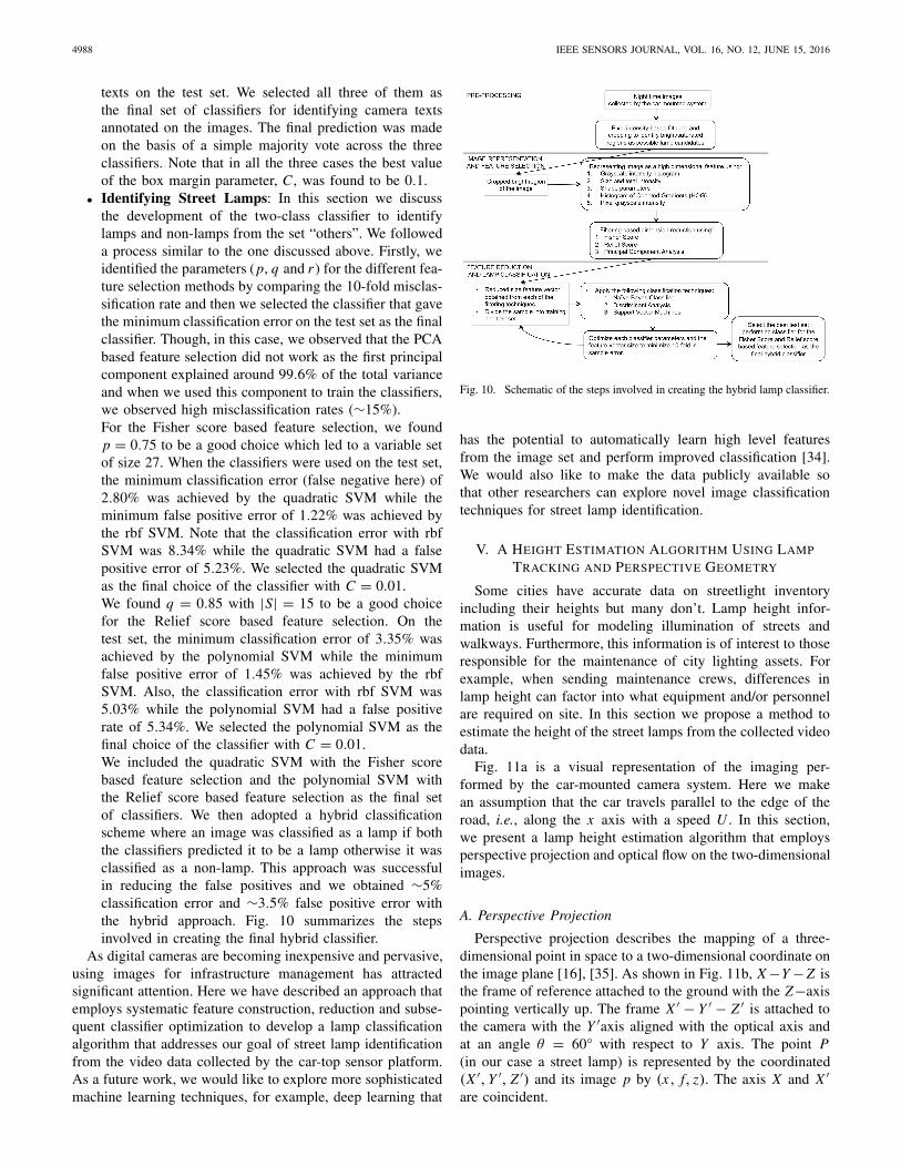
• Identifying Street Lamps: In this section we discussthe development of the two-class classifier to identifylamps and non-lamps from the set “others”. We followeda process similar to the one discussed above. Firstly, weidentified the parameters (p, q and r ) for the different fea-ture selection methods by comparing the 10-fold misclas-sification rate and then we selected the classifier that gavethe minimum classification error on the test set as the finalclassifier. Though, in this case, we observed that the PCAbased feature selection did not work as the first principalcomponent explained around 99.6% of the total varianceand when we used this component to train the classifiers,we observed high misclassification rates (∼15%).For the Fisher score based feature selection, we foundp = 0.75 to be a good choice which led to a variable setof size 27. When the classifiers were used on the test set,the minimum classification error (false negative here) of2.80% was achieved by the quadratic SVM while theminimum false positive error of 1.22% was achieved bythe rbf SVM. Note that the classification error with rbfSVM was 8.34% while the quadratic SVM had a falsepositive error of 5.23%. We selected the quadratic SVMas the final choice of the classifier with C = 0.01.We found q = 0.85 with |S| = 15 to be a good choicefor the Relief score based feature selection. On thetest set, the minimum classification error of 3.35% wasachieved by the polynomial SVM while the minimumfalse positive error of 1.45% was achieved by the rbfSVM. Also, the classification error with rbf SVM was5.03% while the polynomial SVM had a false positiverate of 5.34%. We selected the polynomial SVM as thefinal choice of the classifier with C = 0.01.We included the quadratic SVM with the Fisher scorebased feature selection and the polynomial SVM withthe Relief score based feature selection as the final setof classifiers. We then adopted a hybrid classificationscheme where an image was classified as a lamp if boththe classifiers predicted it to be a lamp otherwise it wasclassified as a non-lamp. This approach was successfulin reducing the false positives and we obtained ∼5%classification error and ∼3.5% false positive error withthe hybrid approach. Fig. 10 summarizes the stepsinvolved in creating the final hybrid classifier.

As digital cameras are becoming inexpensive and pervasive,using images for infrastructure management has attractedsignificant attention. Here we have described an approach thatemploys systematic feature construction, reduction and subse-quent classifier optimization to develop a lamp classificationalgorithm that addresses our goal of street lamp identificationfrom the video data collected by the car-top sensor platform.As a future work, we would like to explore more sophisticatedmachine learning techniques, for example, deep learning that

Fig. 10. Schematic of the steps involved in creating the hybrid lamp classifier.

has the potential to automatically learn high level featuresfrom the image set and perform improved classification [34].We would also like to make the data publicly available sothat other researchers can explore novel image classificationtechniques for street lamp identification.

V. A HEIGHT ESTIMATION ALGORITHM USING LAMP

TRACKING AND PERSPECTIVE GEOMETRY

Some cities have accurate data on streetlight inventoryincluding their heights but many don’t. Lamp height infor-mation is useful for modeling illumination of streets andwalkways. Furthermore, this information is of interest to thoseresponsible for the maintenance of city lighting assets. Forexample, when sending maintenance crews, differences inlamp height can factor into what equipment and/or personnelare required on site. In this section we propose a method toestimate the height of the street lamps from the collected videodata.

Fig. 11a is a visual representation of the imaging per-formed by the car-mounted camera system. Here we makean assumption that the car travels parallel to the edge of theroad, i.e., along the x axis with a speed U . In this section,we present a lamp height estimation algorithm that employsperspective projection and optical flow on the two-dimensionalimages.

A. Perspective Projection

Perspective projection describes the mapping of a three-dimensional point in space to a two-dimensional coordinate onthe image plane [16], [35]. As shown in Fig. 11b, X −Y − Z isthe frame of reference attached to the ground with the Z−axispointing vertically up. The frame X ′ − Y ′ − Z ′ is attached tothe camera with the Y ′axis aligned with the optical axis andat an angle θ = 60° with respect to Y axis. The point P(in our case a street lamp) is represented by the coordinated(X ′, Y ′, Z ′) and its image p by (x, f, z). The axis X and X ′

are coincident.


Fig. 11. Geometry of the car-mounted imaging system.

Assuming an ideal pin hole camera model and using equa-tions of coordinate transformation, for the point P we have

Z ='

sin(θ) + zf

cos(θ)

(X ′ f

x. (5)

We have further assumed that the ground reference frameis attached to the roof of the car. We can now add the heightof the car (Ch) to Z to obtain the height of the lamp post as

hlamp = Ch +'

sin(θ) + zf

cos(θ)

(X ′ f

x

= Ch +'

sin(θ) + zf

cos(θ)

(Y ′. (6)

B. Optical Flow

Optical flow is defined as the apparent motion of thebrightness pattern on an image as the camera moves withrespect to an object or vice versa [16]. Referring to ourimaging geometry of Fig. 11a, let I (x, z, t) be the irradianceat a time t at the image point (x, z). If u(x, z) and w(x, z)are the x and the z components of the optical flow vectors atthat image point and if ∂ t is a small time interval, we makethe following assumption:

I (x, z, t) = I (x + u∂ t, z + w∂ t, t + ∂ t). (7)

Using the Taylor series expansion of (7) and ignoring higherorder terms, we obtain the following optical flow equation atevery pixel (i, j) of a digital image:

Ix ui, j + Izwi, j + It = 0, (8)

where we use a finite difference approximation to computeIx = $

∂ I∂x

%i, j , Iz =

!∂ I∂z

"

i, jand It = $

∂ I∂t

%i, j .

Lucas-Kanade is a popular method for estimating opticalflow that divides the original image into smaller sectionsand assumes a constant velocity in each section [36]. It thensolves a weighted least squares problem in each section byminimizing the following objective:

& &

(i, j )∈(

W 2 (Ix u + Izw + It )2 , (9)

where W is a window function that emphasizes the constraintat the center of each section, ( is the extent of the section

Fig. 12. (a) Example grayscale image frame. (b) Magnitude of x–directionintensity gradient. (c) Magnitude of y–direction intensity gradient.

and (u, w) are the constant optical flow velocities obtainedby minimizing (9). Fig. 12 shows an example image andthe x and y intensity gradient of the image. We observethat the magnitude of the intensity gradient is primarily zerothroughout the image and the pixels with higher magnitudeare confined in a small region surrounding the lamps andother bright regions. This observation prompts a modificationof the Lucas-Kanade method where we first identify the regionof the image where a street lamp is located using our lampclassification technique and then use that region to estimatethe image velocity of the street lamp.

C. Algorithm for Height Estimation

The height of the lamp post as given by (6) is in termsof the unobserved coordinate X ′. Using the pin hole cameramodel we have

X ′ = xY ′

f. (10)

We assume that as the car moves along X ′ axis, Y ′ orthe distance of the lamp from the camera remains constant.Differentiating the left and the right side of (10) with respectto time gives

U = u(x, z)Y ′

f

(⇒ Y ′ = U fu(x, z)

, (11)

where U is the speed of the car along the X axis. Substituting(11) in (6) we get

hlamp = Ch +'

sin(θ) + zf

cos(θ)

(U f

u(x, z), (12)

where z is the image pixel corresponding to the street lamp andu(x, z) is the x component of the optical flow correspondingto the lamp pixel.

As discussed in Section V-B, we find the optical flowvelocity for lamp pixels by first using our lamp classifica-tion algorithm to identify the street lamp and then use theLucas-Kanade formulation by assuming constant (u, w) overthe region corresponding to the street lamp. Assuming W = 1


Fig. 13. Schematic of the steps involved in creating the lamp heightestimation algorithm.

in (9), we obtain the following estimate of u:

u = −

!))I 2

y

" $))Ix It

%−

$) )Ix Iy

% $) )Iy It

%

$) )I 2x% !) )

I 2y

"−

$) )Ix Iy

%2,

(13)

where the summations are taken over all the pixels (i, j) ∈ (l ,which is the region of the image that is identified as a streetlamp. Our lamp identification algorithm also provides thecoordinates of the centroid (xl, zl) of the bounding boxcorresponding to a lamp object. The z−coordinate of thecentroid, zl , was used in height estimate. The car speed, U ,was measured by the OBD-II reader. We then have thefollowing estimate of the height of the street lamp:

hlamp = Ch +'

sin(θ) + zl

fcos(θ)

(U fu

. (14)

We used the following parameters for simulations: Ch = 2 m,θ = 60°, f = 2.8 × 10−3 m and the size of an image pixelto be 3.522 × 10−4 m (which was used to calculate zl ).Applying the above framework to the video data collected inCambridge MA, we estimated the height of the Cobraheadstreet lamps at the intersection of Vassar street and Main streetto be ∼12.9 m with a standard deviation of ∼1.5 m. Cobraheadstreet lamps are typically installed between 12 − 14 m.Fig. 13 summarizes the height estimation algorithm.

VI. LUMINOSITY MAPPING: IMPROVING VEHICLE

LOCATION ESTIMATES THROUGH

GPS-OBD INTEGRATION

Fig. 14 shows a visualization method where the height of thecylinder is proportional to the average illumination measuredacross the sensor array. The location data is provided by theGPS and it specifies the center of the circle. Note that thevisualization overlays the night time data collected during ourdrive-by deployments on the day time images from GoogleEarth.

A key utility of our system is to compare our measurementsagainst the lighting standards. For example, at the intersection

Fig. 14. Two examples of street lighting levels indicated by vertical cylinders.

of Portland St and Broadway in Cambridge MA, the standardrecommends average illuminance of 34 lux with the ratio ofaverage to minimum illuminance being 3 [3]. Across severalmeasurements we found the average illuminance there to be∼25 lux with the ratio of average to minimum illuminancebeing ∼4. Note that our measurements were taken at the car-top level while the standard recommends illumination valuesat street level. As a part of future work, we aim to developtechniques to estimate street level values from car top values.

GPS, which provides absolute geographic location,is typically used to obtain location information of drivingvehicles and has an accuracy of a few meters [37]. DifferentialGPS can have an improved sub-meter accuracy [38]. GPS,in general, suffers from low reliability especially in urbandriving conditions due to multipath effects and poor satellitesignal [39]. Furthermore, as we discussed in Section III-D,we log the data from the GPS at a lower sampling rate ascompared to the IMU and OBD-II scanner. A lower samplingrate limits the spatial resolution of location information. Hencein the context of our sensor platform, we needed to developa robust method for using low frequency, noisy GPS datato accurately estimate vehicle trajectories. We achieved ourobjective by integrating on-board-diagnostics (OBD) car speeddata with the GPS data and the accelerometer measurementsfrom the IMU in an extended Kalman filter (EKF) framework,the details of which can be found in [40].

A different data collection system was used for the resultspresented in this section. The system had a GPS that alloweda maximum sampling frequency of 10 Hz and the data fromthe IMU and the OBD-II reader were directly logged intoa laptop [40]. We collected the original GPS data collectedat 10 Hz and then systematically downsampled it to assessthe impact of a lower frequency GPS data. For each GPSdownsampled sampling rate ( fs ), we execute an on-line EKFestimation, implementing state updates at 10 Hz and storingthe resulting state trajectory.

Fig. 15a and 15b depict two examples of vehicle trajectoryreconstructions with GPS data at fs = 0.2 Hz and 0.05 Hz,respectively, together with a fs = 10 Hz reference trajectoryin black. At a downsampling factor of 50 ( fs = 0.2 Hz) weachieve robust replication of the reference trajectory. At adownsampling factor of 200 ( fs = 0.05 Hz), a segment-wise distortion of the estimated trajectory is observed. Thesesegments mostly exhibit errors in the vehicle heading estimate,while segment lengths show minor deviations.


Fig. 15. Comparison of vehicle reference trajectory (in black) withEKF trajectory estimate (in red) for different GPS sampling times.(a) fs = 0.2 Hz. (b) fs = 0.05 Hz.

Fig. 16. Variation of ϵd with Ts .

We consider two error metrics: relative error in drivendistance estimate (ϵd ) and root mean squared error of positionestimates (ϵr ) [40]. In Fig.16 we report the variation of ϵd asa function of Ts = 1/ fs . For EKF-based trajectory reconstruc-tions, ϵd is lower than 0.1% for Ts < 1 s and lower than 1%for Ts < 50 s. The aggregated distance increments exhibit ahigher driven distance error. The U-shaped distribution of theerrors can be attributed to GPS noise aggregation at low Tsand the failure to capture sufficient path curvature details athigh Ts . On the other hand, our hybrid EKF method providesrobust driven distance estimate that is largely unaffected bythese sources of errors.

Furthermore, we extended our analysis to emulaterandom GPS outage. For every entry in the downsampledGPS-measurement vector, we determined its inclusion in theEKF estimation as the outcome of a Bernoulli trial with acertain probability of not observing the GPS data (denotedby p). We chose p ∈ {1/3, 1/2, 2/3} and for each p ran50 simulations to obtain mean and standard deviation ofthe error metrics. Fig.17a shows that ϵr is acceptable up toTs = 1 s, after which we observe a sharp increase in ϵr .As expected, the error is higher for higher probabilities ofGPS outage. Fig.17b shows a similar trend, though the drivendistance error is acceptable even for higher values of Ts .For driving scenarios where the GPS availability may varyacross the route, this suggests an adaptive sampling strategy.

Fig. 17. Comparison of the performance metrics for different GPS outageprobability (p): (a) ϵr and (b) ϵd . The solid lines indicate the mean of themetric while the dashed lines indicate mean +/− 1

2 standard deviation.

Adjusting the GPS sampling rate in accordance with observedGPS outages will lead to higher accuracy in trajectoryestimation.

VII. RELATED WORK

In the recent past, mobile sensor systems have gainedsignificant attention with the promise to implement large scaleurban monitoring. Google Street View is a benchmark examplewhere images collected by a car driving on the streets arestitched together to create 360° panoramic views [41]. TheCarTel project has shown great promise in monitoring urbancommute times, assessing Wi-Fi deployments and imple-menting automotive diagnostics with deployments spanningmultiple years [42]. Researchers have also deployed vehiclemounted infrared thermography system to address identifica-tion of heat insulation leaks in residential and commercialbuildings [43]. The efforts presented in this paper are in linewith the above theme and vision.

Authors in [44] have recently investigated non-invasivevehicle mounted sensor system to measure street lightinglevels. However their system does not include an OBD-IIsensor and cameras for capturing street lamp images. Thoughthey have discussed in detail the instrumentation challengesand data collection in their field experiments, they have notaddressed signal processing and algorithmic challenges withreal world noisy data.

The advancements in computer vision and imageclassification techniques have encouraged their use invision based urban and environment monitoring applications.There are several challenges to image classification: the sameobject can be imaged with different viewpoints, illumination,occlusion, scale, deformation and background clutter [45].Significant advancements have been made in the classificationof images to identify human faces [46]–[50] which have foundapplications in the areas of surveillance and social networking.Other application areas that have been researched are textrecognition [31]–[33] and car, motorbike or aeroplane


detection [51]–[53]. Researchers have as well exploredcomputer vision techniques to identify street light blackoutsusing simulated data [54].

The first step in image classification involves convertingthe image to a feature vector on which a classification modelcan be learned. The feature vector should have discriminativepower and at the same time should be robust to changes inpose, illumination, scaling and background clutter. Researchershave explored various object representation and feature con-struction schemes such as edge descriptors, part and structuremodels, constellation models, shape features, histogram oforiented gradients, bag of visual words, etc. [45], [55], [56].

The next step involves developing a learning algorithmwhich can be divided into generative and discriminative meth-ods. In a generative model a joint distribution of the featurevector (x) and the class label (c) is learned as p(c, x) while ina discriminative model a conditional distribution p(c|x) or aninput-output relationship c = f (x) is learned. Both generativemodels (e.g. mixture models, naive Bayes, topic models) anddiscriminative models (e.g. support vector machines (SVM),nearest neighbors, conditional random fields and neural net-works) have been used for image classification applications[23]–[30], [45], [55].

Typically the size of the feature vector in an image classifi-cation task is large and a feature selection step is implementedbefore developing a learning algorithm. Feature selection ordimensionality reduction has been studied extensively in themachine learning community and some of its key benefitsinclude: better understanding and visualization of data, fastertraining and developing computationally efficient classifiers,reducing the curse of dimensionality and providing better gen-eralization performance. The feature selection techniques canbe broadly divided into three different categories: wrappers,filters and embedded methods [17]–[22].

Optical flow for motion tracking has been studiedextensively in the computer vision community and hasfound several applications in surveillance, three-dimensionalshape reconstruction, video compression, medical imagingetc. [16], [57], [58].

Researchers have made significant progress in developingsensor fusion algorithms for combining GPS data with inertialmeasurement units (IMU) to improve location estimates. Thesemethods typically involve a vehicle motion model, a sensorobservation model and a Kalman filter like framework toimprove GPS location estimates [40], [59], [60].

Use of urban road map information and map-matchingtechniques have been studied to further improve locationestimates [61]–[64]. Map-matching has the potential to beintegrated with our work to improve vehicle location errors.Furthermore, map data can be used to construct prior estimateson lamp locations which can reduce false negatives andpositives. Lamp location errors can also be reduced throughrepeated measurements over time to increase the confidenceinterval of the estimated location.

VIII. CONCLUSION AND FUTURE WORK

In this paper we have presented a car-top sensor systemfor monitoring urban street light infrastructure. Our sensor

system is built of an array of lux meters for light intensitymapping and security cameras to identify street lamps fromdifferent light sources. Dedicated microcontroller and DVRsystems help in logging data from these sensors. Additionally,we gathered and combined data from GPS, IMU and OBD-IIsensors to obtain improved location estimates which enhancethe quality of mapping and improve accuracy of lamp inven-torying. The main challenge with the camera images is toseparate street lamps from other shining objects. We developeda supervised learning method to identify street lamps incropped images from other light sources. We used Fisher scoreand Relief score as supervised filters and principal componentanalysis (PCA) as an unsupervised filter in feature selection.We demonstrated a classification accuracy of 95% and a falsepositive rate of 3.5% with support vector machines. Once thelamps were identified, we developed a perspective geometrybased methodology to estimate height of lamps, which canhelp in developing a stock of street lamp inventory. We furtherdemonstrated average illumination mapping with the lightsensor data and improved location estimates.

To summarize, we have described that our final prototypeis capable of collecting data reliably under real driving condi-tions. We have also discussed the algorithms and their founda-tions that enable us to make inferences from the collected realworld noisy data. Indeed our efforts went through several itera-tions, the details of which can be found in the PhD thesis [10].

The car-top sensor system presents several possible direc-tions for future work. For example, light intensity mappingand street lamp inventory can help in identifying low lightintensity areas and find candidate locations for adding streetlamps. This system can aid to monitor current health oflighting infrastructure and maintenance needs. It can also beused to verify existing lamp inventory data and create newones in a scalable way. As noted before, we would like todevelop techniques to estimate street level illumination levelsfrom car top measurements. Furthermore, we would like toestablish accuracy and error bounds to compare our processwith the measurement norms detailed in the lighting standards.Correlating light intensity maps with other social indicatorssuch as crime frequency can recommend necessary actions.Our eventual goal is to develop a semi-live virtual three-dimensional street lighting model at urban scale that willenable citizens and decision makers to assess and optimizeperformance of nighttime street lighting.

ACKNOWLEDGMENT

The authors would also like to thank members of the FieldIntelligence Lab, MIT for useful discussions.

REFERENCES

[1] “Street lighting retrofit projects: Improving performance, while reducingcosts and greenhouse gas emissions, Clinton Climate Initiative, Tech.Rep., 2010.

[2] Road Lighting—Part 2: Performance Requirements, European Stan-dard EN 13201-2, European Committee for Standardization, 2003.

[3] IES RP-8-14: Roadway Lighting (ANSI Approved), Illuminating Eng.Society Std. IES RP-8-14, Wall Street, NY, USA, 2014.

[4] L.A. Faces 72-Million USD Budget Shortfall. [Online]. Available:http://articles.latimes.com/2011/dec/03/local/la-me-city-budget-shortfall-20111203


[5] C. Jing, D. Shu, and D. Gu, “Design of streetlight monitoring and controlsystem based on wireless sensor networks,” in Proc. 2nd IEEE Conf. Ind.Electron. Appl. (ICIEA), May 2007, pp. 57–62.

[6] X.-M. Huang, J. Ma, and L. E. Leblanc, “Wireless sensor network forstreetlight monitoring and control,” Proc. SPIE, vol. 5440, pp. 313–321,Apr. 2004.

[7] Sign Up for the LightGrid Pilot Program Today! [Online]. Available:http://www.gelighting.com/LightingWeb/na/images/CTRL012-GE-LightGrid-Pilot-Program-Sell-Sheet_tcm201-104308.pdf

[8] D. Bhadauria, O. Tekdas, and V. Isler, “Robotic data mules for col-lecting data over sparse sensor fields,” J. Field Robot., vol. 28, no. 3,pp. 388–404, 2011.

[9] M. Di Francesco, S. K. Das, and G. Anastasi, “Data collection inwireless sensor networks with mobile elements: A survey,” ACM Trans.Sensor Netw., vol. 8, no. 1, p. 7, Aug. 2011.

[10] S. Kumar, “Mobile sensor systems for field estimation and ‘hot spot’identification,” Ph.D. dissertation, Dept. Mech. Eng., Massachusetts Inst.Technol., Cambridge, MA, USA, 2014.

[11] N. Dalal and B. Triggs, “Histograms of oriented gradients for humandetection,” in Proc. IEEE Comput. Soc. Conf. Comput. Vis. PatternRecognit., Jun. 2005, vol. 1. no. 1, pp. 886–893.

[12] Q. Zhu, M.-C. Yeh, K.-T. Cheng, and S. Avidan, “Fast human detectionusing a cascade of histograms of oriented gradients,” in Proc. IEEEComput. Soc. Conf. Comput. Vis. Pattern Recognit., vol. 2, Jun. 2006,pp. 1491–1498.

[13] P. E. Rybski, D. Huber, D. D. Morris, and R. Hoffman, “Visualclassification of coarse vehicle orientation using histogram of orientedgradients features,” in Proc. IEEE Intell. Vehicles Symp. (IV), Jun. 2010,pp. 921–928.

[14] L. Hu, W. Liu, B. Li, and W. Xing, “Robust motion detection usinghistogram of oriented gradients for illumination variations,” in Proc.2nd Int. Conf. Ind. Mechatron. Autom. (ICIMA), vol. 2, May 2010,pp. 443–447.

[15] O. Déniz, G. Bueno, J. Salido, and F. De la Torre, “Face recognitionusing histograms of oriented gradients,” Pattern Recognit. Lett., vol. 32,no. 12, pp. 1598–1603, 2011.

[16] B. K. P. Horn, Robot Vision (MIT Electrical Engineering and ComputerScience). Cambridge, MA, USA: MIT Press, 1986.

[17] I. Guyon and A. Elisseeff, “An introduction to variable and featureselection,” J. Mach. Learn. Res., vol. 3, pp. 1157–1182, Jan. 2003.

[18] Y. Saeys, I. Inza, and P. Larrañaga, “A review of feature selec-tion techniques in bioinformatics,” Bioinformatics, vol. 23, no. 19,pp. 2507–2517, 2007.

[19] H. Peng, F. Long, and C. Ding, “Feature selection based on mutualinformation criteria of max-dependency, max-relevance, and min-redundancy,” IEEE Trans. Pattern Anal. Mach. Intell., vol. 27, no. 8,pp. 1226–1238, Aug. 2005.

[20] J. Fan and J. Lv, “A selective overview of variable selection inhigh dimensional feature space,” Statist. Sinica, vol. 20, no. 1,pp. 101–148, 2010.

[21] M. Pal and G. M. Foody, “Feature selection for classification ofhyperspectral data by svm,” IEEE Trans. Geosci. Remote Sens., vol. 48,no. 5, pp. 2297–2307, May 2010.

[22] I. A. Gheyas and L. S. Smith, “Feature subset selection in largedimensionality domains,” Pattern Recognit., vol. 43, no. 1, pp. 5–13,2010.

[23] D. D. Lewis, “Naive (Bayes) at forty: The independence assumptionin information retrieval,” in Mach. Learning: ECML. Berlin, Germany:Springer-Verlag, 1998, pp. 4–15.

[24] J. Ren, S. D. Lee, X. Chen, B. Kao, R. Cheng, and D. Cheung, “NaiveBayes classification of uncertain data,” in Proc. 9th IEEE Int. Conf. DataMining (ICDM), 2009, pp. 944–949.

[25] T. Calders and S. Verwer, “Three naive Bayes approaches fordiscrimination-free classification,” Data Mining Knowl. Discovery,vol. 21, no. 2, pp. 277–292, 2010.

[26] C. J. Huberty, Applied Discriminant Analysis. New York, NY, USA:Wiley, 1994.

[27] S. Mika, G. Ratsch, J. Weston, B. Scholkopf, and K. R. Mullers, “Fisherdiscriminant analysis with kernels,” in Proc. 9th IEEE Signal Process.Soc. Workshop Neural Netw. Signal Process., 1999, pp. 41–48.

[28] C. J. C. Burges, “A tutorial on support vector machines for pat-tern recognition,” Data Mining Knowl. Discovery, vol. 2, no. 2,pp. 121–167, 1998.

[29] C.-C. Chang and C.-J. Lin, “LIBSVM: A library for support vectormachines,” ACM Trans. Intell. Syst. Technol., vol. 2, no. 3, p. 27, 2011.

[30] G. Mountrakis, J. Im, and C. Ogole, “Support vector machines in remotesensing: A review,” ISPRS J. Photogram. Remote Sens., vol. 66, no. 3,pp. 247–259, 2011.

[31] Y. Amit and D. Geman, “Shape quantization and recognition withrandomized trees,” Neural Comput., vol. 9, no. 7, pp. 1545–1588, 1997.

[32] Y. Amit and D. Geman, “A computational model for visual selection,”Neural Comput., vol. 11, no. 7, pp. 1691–1715, 1999.

[33] S. Espana-Boquera, M. J. Castro-Bleda, J. Gorbe-Moya, andF. Zamora-Martinez, “Improving offline handwritten text recognitionwith hybrid HMM/ANN models,” IEEE Trans. Pattern Anal. Mach.Intell., vol. 33, no. 4, pp. 767–779, Apr. 2011.

[34] Q. V. Le et al. (2011). “Building high-level features usinglarge scale unsupervised learning.” [Online]. Available:http://arxiv.org/abs/1112.6209

[35] R. Collins. (2007). CSE/EE486 Computer Vision I: Introduction toComputer Vision. [Online]. Available: http://www.cse.psu.edu/~rcollins/CSE486/

[36] S. Baker and I. Matthews, “Lucas–Kanade 20 years on: A unifyingframework,” Int. J. Comput. Vis., vol. 56, no. 3, pp. 221–255, 2004.

[37] L. L. Arnold and P. A. Zandbergen, “Positional accuracy of the wide areaaugmentation system in consumer-grade GPS units,” Comput. Geosci.,vol. 37, no. 7, pp. 883–892, Jul. 2011.

[38] L. S. Monteiro, T. Moore, and C. Hill, “What is the accuracy of DGPS?”J. Navigat., vol. 58, no. 2, pp. 207–225, 2005.

[39] P. Zhang, J. Gu, E. E. Milios, and P. Huynh, “Navigation withIMU/GPS/digital compass with unscented Kalman filter,” in Proc. IEEEInt. Conf. Mechatron. Autom., vol. 3. Niagara Falls, Canada, Jul. 2005,pp. 1497–1502.

[40] S. Kumar, J. Paefgen, E. Wilhelm, and S. E. Sarma, “Integrating on-board diagnostics speed data with sparse gps measurements for vehicletrajectory estimation,” in Proc. SICE Annu. Conf. (SICE), Nagoya, Japan,Sep. 2013, pp. 2302–2308.

[41] D. Anguelov et al., “Google street view: Capturing the world at streetlevel,” Computer, vol. 43, no. 6, pp. 32–38, Jun. 2010.

[42] B. Hull et al., “CarTel: A distributed mobile sensor computing system,”in Proc. 4th Int. Conf. Embedded Netw. Sensor Syst., 2006, pp. 125–138.

[43] L. N. Phan, “Automated rapid thermal imaging systems technology,”Ph.D. dissertation, Dept. Mech. Eng., Massachusetts Inst. Technol.,Cambridge, MA, USA, 2012.

[44] H. C. Lee and H. B. Huang, “A low-cost and noninvasive system for themeasurement and detection of faulty streetlights,” IEEE Trans. Instrum.Meas., vol. 64, no. 4, pp. 1019–1031, Apr. 2015.

[45] L. Fei-Fei, R. Fergus, and A. Torralba. (2005). Recognizing andLearning Object Categories. [Online]. Available: http://people.csail.mit.edu/torralba/shortCourseRLOC/

[46] P. Viola and M. J. Jones, “Robust real-time object detection,” Int. J.Comput. Vis., vol. 4, pp. 1–30, Jul. 2001.

[47] M.-H. Yang, “Kernel eigenfaces vs. Kernel fisherfaces: Face recognitionusing Kernel methods,” in Proc. 5th IEEE Int. Conf. Autom. FaceGesture Recognit., May 2002, pp. 215–220.

[48] W. Zhao, R. Chellappa, P. J. Phillips, and A. Rosenfeld, “Face recog-nition: A literature survey,” ACM Comput. Surv., vol. 35, no. 4,pp. 399–458, 2003.

[49] P. Viola and M. J. Jones, “Robust real-time face detection,” Int. J.Comput. Vis., vol. 57, no. 2, pp. 137–154, 2004.

[50] S. Z. Li and A. K. Jain, Eds., Handbook of Face Recognition. Nagoya,Japan: Springer, 2011.

[51] H. Schneiderman and T. Kanade, “Object detection using the statisticsof parts,” Int. J. Comput. Vis., vol. 56, no. 3, pp. 151–177, 2004.

[52] S. Agarwal and D. Roth, “Learning a sparse representation forobject detection,” in Computer Vision—ECCV. Berlin, Germany:Springer-Verlag, 2002, pp. 113–127.

[53] A. Vedaldi and A. Zisserman. (2011). Image Classification Practical.[Online]. Available: http://www.robots.ox.ac.uk/~vgg/share/practical-image-classification.htm

[54] P. N. Zanjani, M. Bahadori, and M. Hashemi, “Monitoring and remotesensing of the street lighting system using computer vision and imageprocessing techniques for the purpose of mechanized blackouts (devel-opment phase),” in Proc. 22nd Int. Conf. Exhibit. Electr. Distrib., 2013,pp. 1–4.

[55] A. Torralba. (2012). 6.869: Advances in Computer Vision. [Online].Available: http://6.869.csail.mit.edu/fa12/

[56] D. Zhang and G. Lu, “Review of shape representation and descriptiontechniques,” Pattern Recognit., vol. 37, no. 1, pp. 1–19, Jan. 2004.

[57] T. Senst, V. Eiselein, and T. Sikora, “Robust local optical flow for featuretracking,” IEEE Trans. Circuits Syst. Video Technol., vol. 22, no. 9,pp. 1377–1387, Sep. 2012.


[58] H. Yang, L. Shao, F. Zheng, L. Wang, and Z. Song, “Recent advancesand trends in visual tracking: A review,” Neurocomputing, vol. 74,no. 18, pp. 3823–3831, Nov. 2011.

[59] W. Ding, J. Wang, C. Rizos, and D. Kinlyside, “Improving adaptiveKalman estimation in GPS/INS integration,” J. Navigat., vol. 60, no. 3,pp. 517–529, 2007.

[60] J. Georgy, T. Karamat, U. Iqbal, and A. Noureldin, “Enhanced MEMS-IMU/odometer/GPS integration using mixture particle filter,” GPS Solu-tions, vol. 15, no. 3, pp. 239–252, 2011.

[61] C. Smaili, M. E. E. Najjar, and F. Charpillet, “Multi-sensor fusionmethod using dynamic Bayesian network for precise vehicle localiza-tion and road matching,” in Proc. 19th IEEE Int. Conf. Tools Artif.Intell. (ICTAI), vol. 1, Oct. 2007, pp. 146–151.

[62] M. A. Quddus, W. Y. Ochieng, and R. B. Noland, “Current map-matching algorithms for transport applications: State-of-the art andfuture research directions,” Transp. Res. C, Emerg. Technol., vol. 15,no. 5, pp. 312–328, 2007.

[63] J. S. Greenfeld, “Matching GPS observations to locations on a digitalmap,” in Proc. Transp. Res. Board 81st Annu. Meeting, 2002.

[64] P. Newson and J. Krumm, “Hidden Markov map matching throughnoise and sparseness,” in Proc. 17th ACM SIGSPATIAL Int. Conf. Adv.Geographic Inf. Syst. (GIS), New York, NY, USA, 2009, pp. 336–343.

Sumeet Kumar received the bachelor’s degree fromthe Indian Institute of Technology Kanpur, the M.S.degree in mechanical engineering from the Massa-chusetts Institute of Technology (MIT), in 2009,and the Ph.D. degree in mechanical engineeringfrom MIT in 2014. He is currently a Quantita-tive Researcher with Dean Capital Investments. Hisresearch interests include machine learning, statisti-cal signal processing, data science, sensor systems,and thermal modeling. He received the PappalardoFellowship and the Academic Excellence Awards in

2005 and 2006.

Ajay Deshpande received the B.Tech. and M.Tech.degrees from the Indian Institute of TechnologyBombay in 2001, and the master’s degrees inmechanical engineering, and electrical engineeringand computer science and the Ph.D. degree inmechanical engineering from the MassachusettsInstitute of Technology (MIT), in 2006 and 2008,respectively. He was a Post-Doctoral Associate withthe Laboratory for Manufacturing and Productivity,MIT. He is currently a Research Staff Memberwith the IBM Thomas J. Watson Research Center,

Yorktown Heights, NY. He was a recipient of the MIT Presidential Fellowship.

Stephen S. Ho received the B.Sc. degree from Cor-nell University, and the M.S. and Ph.D. degrees fromthe Massachusetts Institute of Technology (MIT),Cambridge, MA, USA, all in mechanical engineer-ing. He has been a Research Scientist with theField Intelligence Laboratory, MIT, since 2007. Hisresearch interests center around the application ofinformation toward improving systems, processes,and resource management. His current researchincludes sensors and inference of vehicles and vehi-cle traffic, lighting and municipal assets for urban

environments, and energy efficiency. His Ph.D. research evaluated the impactrich RFID information has on warehouse operations and the opportunities forincreased efficiency that stem from that additional information.

Jason S. Ku is currently pursuing the Ph.D. degreewith the Department of Mechanical Engineering,Massachusetts Institute of Technology. He primarilystudies computational geometry, particularly ques-tions involving the relationship between two andthree dimensions. His research topics include thedesign and fabrication of static and transformablefolding structures from sheet-like material, 3-Dobject reconstruction algorithms from lower dimen-sional projections, and 3-D projection.

Sanjay E. Sarma received the bachelor’s degreefrom the Indian Institute of Technology, the master’sdegree from Carnegie Mellon University, and thePh.D. degree from the University of California atBerkeley. He was the Fred Fort Flowers (1941) andDaniel Fort Flowers (1941) Professor of MechanicalEngineering at MIT. He is the first Dean of DigitalLearning at MIT. He co-founded the Auto-ID Centerat MIT and developed many of the key technologiesbehind the EPC suite of RFID standards now usedworldwide. He was also the Founder and CTO of

OATSystems, which was acquired by Checkpoint Systems (NYSE: CKP) in2008. He serves on the Boards of GS1, EPCglobal, and several startup compa-nies, including Senaya and ESSESS. He also work with Schlumberger OilfieldServices, Aberdeen, U.K., and the Lawrence Berkeley Laboratories, Berkeley,CA. He has authored over 75 academic papers in computational geometry,sensing, RFID, automation, and CAD, and is a recipient of numerous awardsfor teaching and research, including the MacVicar Fellowship, the BusinessWeek eBiz Award, and the Informationweek’s Innovators and InfluencersAward. He advises several national governments and global companies.

ieee sensors journal, vol. 16, no. 12, june 15, 2016 …jasonku/pdf/lighting_ieee2016.pdfieee...

Documents