ieee transaction on image processing 1 …ieee transaction on image processing 1 joint hierarchical...

IEEE TRANSACTION ON IMAGE PROCESSING 1

Joint Hierarchical Category Structure Learning andLarge-Scale Image Classification

Yanyun Qu, Member, IEEE, Li Lin, Fumin Shen, Chang Lu,Yang Wu, Yuan Xie, Member, IEEE, Dacheng Tao, Fellow, IEEE,

Abstract—We investigate the scalable image classification prob-lem with a large number of categories. Hierarchical visual datastructures are helpful for improving the efficiency and perfor-mance of large-scale multi-class classification. We propose a novelimage classification method based on learning hierarchical inter-class structures. Specifically, we first design a fast algorithmto compute the similarity metric between categories, basedon which a visual tree is constructed by hierarchical spectralclustering. Using the learned visual tree, a test sample labelis efficiently predicted by searching for the best path over theentire tree. The proposed method is extensively evaluated on theILSVRC2010 and Caltech 256 benchmark datasets. Experimentalresults show that our method obtains significantly better categoryhierarchies than other state-of-the-art visual tree-based methodsand, therefore, much more accurate classification.

Index Terms—Hierarchical learning, large-scale image classi-fication, deep features, visual tree, N-best path

I. INTRODUCTION

GREAT progresses have been witnessed in image classifi-cation [4], [30], [31], [34], [36]–[38], [49], [57], [58]

in recent years. Especially, large-scale image classificationhas achieved remarkable developments [32], [39], [43], [48],[60]. Nevertheless, most state-of-the-art methods have thefollowing two limitations: 1) inter-class taxonomic relation-ships are neglected; thus, the hierarchical structure of multipleclasses cannot be generated and visualized; and 2) multi-classclassification decision-making is “flat”, making computationinefficient.

With respect to visual hierarchical relationships, as the ex-plosive rise in diverse social media data extends beyond directadministration by individual users, a proper hierarchical struc-ture could make it easier for users to capture the distribution ofimage data such that they can effectively manage and organizetheir data. Moreover, it is natural to organize data accordingto their relationships and form a hierarchical structure. For

Yanyun Qu, Li Lin, and Chang Lu are with the Department ofComputer Science, Xiamen University, Xiamen, 361005, China (e-mail:[email protected]).

Fumin Shen is with the School of Computer Science and Engineering,University of Electric Science and technology of China, Chengdu, 611731,China ([email protected]).

Yang Wu is with Institute for Research Initiatives, Nara Institute of Scienceand Technology, Japan ([email protected]).

Yuan Xie is with Research Center of Precision Sensing and ControlInstitute of Automation, Chinese Academy of Sciences, Beijing, 100190,China (email:[email protected]).

Dacheng Tao is with the Centre for Artificial Intelligence and the Fac-ulty of Engineering and Information Technology, University of Technol-ogy Sydney, 81 Broadway Street, Ultimo, NSW 2007, Australia (email:[email protected])

example, ImageNet [1] is organized hierarchically accordingto a high-level semantic lexical database called WordNet [41],which classifies objects in the natural world according tophylum, class, order, family, genus, and species, i.e., a well-established hierarchy.

With respect to multi-class classification, most methodssimply directly adopt a flat scheme, i.e., one-vs.-all or one-vs.-one classifiers, making prediction time-consuming. For Nclasses, one-vs.-all needs to compute N classifiers and one-vs.-one needs to compute N(N−1)/2 classifiers when predictinga query image. When N is large, the two flat methods are notefficient. Thus, we seek hierarchical structure to improve theefficiency of multi-class prediction which requires O(logKN)classifiers for a tree with K branches in each layer. Moreover,real-world object classes tend to have strong hierarchicalrelationships, and it is usually easier for humans to distinguishcoarse-level categories than fine-grained subcategories. Givena hierarchical structure, classification can be performed in acoarse-to-fine manner, which improves prediction efficiencyand accuracy. To this end, we propose an efficient multi-class classification framework based on hierarchical categorystructure learning.

The first challenge is how to apply a hierarchical structureto visual data. Hierarchical classification methods typically de-pend on a given hierarchical structure, e.g., WordNet for Ima-geNet. However, the construction of ImageNet was demandingand time-consuming. In real world scenarios, knowledge abouthow to organize data hierarchically is often limited; we usuallyonly know some coarse and obscure dataset cues. Thus, it isdifficult to utilize high-level semantics to construct a hierar-chical structure. Moreover, there is no evidence to suggest thatclass prediction according to hierarchical semantics improvesperformance; the classification accuracy can be low even whena hierarchical semantic structure is used [29], [53]. This isprobably due to the semantic gap between high-level semanticsand low-level features. Thus, we propose making hierarchicalclassification dependent on a visual tree constructed usingvisual features but not predefined rules.

Performing hierarchical inference based on the visual hi-erarchical structure is also challenging. Greedy learning is atypical way to solve classification prediction using visual treemodels [6], [29], [62]. However, while relatively intuitive, thegreedy approach does not prevent error propagation; that is, ifa mistake is made in an intermediate node, the prediction resultis then destined to be wrong. To overcome this drawback,we transform the problem of class prediction into a task offinding the optimal path of a visual tree by maximizing a joint

arX

iv:1

709.

0507

2v1

[cs

.CV

] 1

5 Se

p 20

17


probability.The main contributions of our approach are as follows:1) We propose a fast approach for computing the between-

category similarity metric, based on which hierarchicalspectral clustering is used to construct the visual tree.

2) To avoid error propagation, we transform the classprediction problem into a path-searching problem usinga novel method that we call N-best path. N-best pathis an approximation of the optimal path solved by themaximum joint probability of candidate paths. Ratherthan finding only one path, we retain candidate pathscorresponding to the top N largest joint probabilities.Compared to traditional greedy learning methods, the N-best path algorithm effectively avoids error propagationand improves prediction efficiency.

3) The proposed classification framework is extensivelyevaluated with respect to different image representationsincluding hand-crafted features and recently developeddeep features. Furthermore, we compare the proposedapproach with several other visual tree-based algorithmson two large datasets: ILSVRC2010 and Caltech 256.Our method produces significantly better category hier-archies and thus improves classification accuracy com-pared to the previous state-of-the-art methods.

The remainder of this paper is organized as follows. Weintroduce related work in Section II. In Section III, we con-struct a visual tree model and detail the N-best path algorithmfor label inference depending on the visual tree. Experimentalresults are presented in Section IV, and we conclude in SectionV.

II. RELATED WORK

A. Hierarchical learning

There are two groups of hierarchical learning approaches:taxonomy-related methods and taxonomy-independent meth-ods. Motivated by the success of taxonomies in web orga-nization and text document categorization, many computervision researchers have utilized taxonomies to organize large-scale image collections or improve visual system performance.For instance, Li et al. [1] constructed ImageNet according toWordNet, a semantic hierarchy taxonomy unrelated to visualeffects. Although WordNet has been widely applied to imageclassification [53], the visual attributes are always ignored.

There are precedents that learning visual hierarchical struc-tures can be helpful for image classification [13], [14]. Sivicet al. [51] used a hierarchical Latent Dirichlet Allocation(hLDA) on Bag Of Word (BOW) [9] with SIFT local featuresto discover a hierarchical structure from unlabeled images,which simultaneously facilitated image classification and seg-mentation, while Bart et al. [5] utilized an unsupervisedBayesian model on BOW with color-space histograms to learna tree structure. Both methods were tested on moderate-scaledatasets; their performance on large-scale image data is lessclear. Moreover, they focused on image classification but didnot visualize the hierarchical inter-class relationship. To doso, some researchers [6], [24], [33] have built hierarchicalmodels based on confusion matrices obtained or computed

by the output of image categorization or object classificationusing N one-vs.-all SVM classifiers. Griffin et al. [24] con-structed a binary branch tree to improve visual categorization,Bengio et al. [6] built a label-embedding tree for multi-classclassification, while Liu et al. [33] constructed a probabilisticlabel tree for large-scale classification. Gao, et al. [19] builtthe relaxed hiearchical structure which allows the confusionclasses belong to more than one node. However, hierarchicallearning methods based on confusion matrices suffer from twomain limitations: 1) computation of the confusion matrix usinga one-vs.-all SVM is time consuming; and 2) the confusionmatrix may not be reliable due to unbalanced training data.Visual trees constructed by clustering produce an intuitivehierarchical structure [12], [29], [40], [62] and have attractedmore and more attention. Zhou et al. [62] utilized AP clus-tering and Lei et al. [29] implemented spectral clustering toconstruct visual trees. Although results were promising withthese methods, there is still plenty of room for improvementin hierarchical learning.

There are three important components to hierarchical learn-ing: image representation, hierarchical structure construction,and multi-class classification inference. The greedy learn-ing method is typically utilized for class prediction. Mosthierarchical classification approaches [6], [11], [16], [24],[40], [50] make predictions in each layer by maximizing theclassification probability. However, as noted above, inferencesfrom greedy learning do not prevent error propagation. Incontract, our method provides a distribution of hierarchicalmemberships for image categories based on spectral clustering,in which the best path algorithm is developed to avoid errorpropagation. The closest related work is [53], where thebest path is learned by the structured SVM, leading to highcomputational complexity. We make classification predictionsbased on the best path algorithm depending on the hierarchicalstructure.

B. Image representation

Many image representation methods [31], [36] have beenused in computer vision with the BOW model, one of the mostpopular tools for image representation in image classification[22], [46], [56], image annotation [38] and image segmen-tation. The main advantage of the BOW model is that it isuniversal for image classification, meaning that it can representgeneric classes of objects other than those for special objectrecognition (e.g., Haar-like features are especially effectivefor face detection). Usually, a BOW model includes threeimportant components: 1) local feature extraction, 2) visualfeature encoding, and 3) the classifier design. Local featureextraction is a prerequisite for image classification. The morediscriminative the features, the better the image classificationperformance. Most common local features such as SIFT [35]and HOG [10] are carefully engineered.

In view of the need for a visual dictionary and encoding,K-means is traditionally used to construct a visual dictionaryand the cluster centers are treated as the visual words. K-means is an unsupervised method, so the visual dictionarylacks discriminatory power. Therefore, efforts have been made


to encode discriminative features. Yang et al. [59] used sparserepresentations to encode the features, leading to improve-ments in dictionary learning for multi-class classification withlarge numbers of classes [8], [16], [18], [50], [62]. More ad-vanced methods have emerged over recent years such as local-constrained linear coding [55], super-vector coding [63], andFisher vectors [45]. Although these methods have generallyimproved the discrimination of visual features, they dependon experts. More flexible and effective features are requiredfor large-scale image classification.

Deep features learned by deep learning have become moreprevalent over recent years and can be obtained in an end-to-end manner without much human intervention. They havebeen highly successful for audio and text recognition. Lecunet al. [28] designed a convolutional neural network (CNN)for object recognition that combined feature extraction withclassifier design. Krizhevsky et al. [25] constructed a deepCNN for large-scale image classification, while Christianimproved GoogLeNet and developed the Inception V3 model[54]. However, there is a paucity of literature on how deepfeatures influence hierarchical learning. Here, we bridge thisgap by exploring the effect of deep features on hierarchicallearning.

III. HIERARCHICAL LEARNING ALGORITHM OVERVIEW

The framework of our approach is shown in Fig.1. It hastwo components: visual tree construction and class prediction.In the former, an image representation is made for each image,after which an affinity matrix is computed that measuresthe inter-class similarity. The hierarchical category structureis then found according to the affinity matrix by spectralclustering. A visual tree model is made by assigning a weightto each edge. During testing, a query image is first representedbefore a prediction being made according to the visual treemodel. We detail our approach below.

A. Visual Tree Construction

In this subsection, we detail how to construct the visual tree.There are two main components to our visual tree constructionalgorithm: 1) the similarity metric between two categories, and2) hierarchical clustering for visual tree construction. Aligningthe inter-class semantic similarity with the inter-class visualsimilarity is still an unsolved issue in the multimedia andcomputer vision communities. Human perceptual factors maybe important for designing a more suitable cross-modal align-ment framework. Some methods [6], [33] have constructedthe visual tree according to the confusion matrix obtained bytraining a one-vs.-all classifier for all N classes. However,these methods are computationally demanding.

Affinity matrix computation. In this paper, we computean affinity matrix based on a new inter-class distance metricto construct a visual tree. This produces an algorithm thatis much faster than those using traditional pairwise distances.Moreover, the proposed inter-class distance metric can be usedto illustrate the relationship between two types of inter-classdistance metric: the distance based on two class means [15],

[62] and the distance based on the pairwise distance of twoclasses [12], [29].

Suppose that there are N image categories{C1, C2, · · · , CN}, and the ith image category Ci containsNi images represented by the features {Iil }

Ni

l=1. The similaritymetric based on the pairwise distance between two classes isformulated as,

dis(Ci, Cj) = sqrt(1

NiNj

∑s

∑t

‖ Iis − Ijt ‖2) (1)

We take the norm operation as a unit, and (1) requires NiNj

norm operations. To reduce the computation of (1), we inferit as,

dis2(Ci, Cj) =1

NiNj

∑s

∑t

‖ (Qi−∆Iis)− (Qj −∆Ijt ) ‖2

(2)where ∆Iis = Qi − Iis is the difference between the imageIis and the mean of their class Qi, where Qi = 1

Ni

∑Ni

l=1 Iil .

Furthermore, we substitute the property∑Ni

s=1 ∆Iis = 0 into(2), obtaining a new distance formula,

dis2(Ci, Cj)

=1

NiNj

Ni∑s=1

Nj∑t=1

‖ (Qi −Qj)− (∆Iis −∆Ijt ) ‖2

=‖ Qi −Qj ‖2 −2

NiNj‖Qi −Qj‖

Ni∑s=1

Nj∑t=1

(∆Iis −∆Ijt )

+1

NiNj

Ni∑s=1

Nj∑t=1

(∆Iis −∆Ijt )2

= ‖Qi −Qj‖2 +1

Ni

Ni∑s=1

(∆Iis)2 +

1

Nj

Nj∑t=1

(∆Iit)2

= ‖Qi −Qj‖2 + σ2i + σ2

j

(3)

where σ2i = 1

Ni

∑Ni

l=1 ‖Iil −Qi‖2 is the square of the varianceof the category Ci. (3) requires only Ni + Nj + 1 normoperations which are much less than those needed by (1).Considering that the variance can be pre-computed for eachcategory, the computational cost is the same as that for thedistance between class means.

Though the inference of (3) is simple, it obviously improvesthe computation of the inter-class distance. More importantly,it illustrates the core of the inter-class distance. The proposedsimilarity metric is related to both between-class scatter andwithin-class scatter. If the two centers of pairwise classes arecloser and the divergence of the two classes are smaller, thesimilarity of two classes is bigger.

We construct a visual affinity graph by using the similaritymetric between categories. Hierarchical spectral clustering[42] is then applied to construct a visual tree. The elementof the affinity matrix is computed as,

Aij = exp(−dis(Ci, Cj)

δij) (4)

where δij is the self-tuning parameter according to [46].


Fig. 1. The hierarchical learning framework. a) Image representation. b) Affinity network construction for similarity comparison between two categories basedon a similarity metric. c) Visual tree construction via hierarchical spectral clustering. d) Image representation for a query image. e) Label inference accordingto the visual tree model.

Visual tree construction. We adopt the top-down strategyto construct the visual tree. Each node in the tree is partitionedrecursively during the construction procedure. The root nodev is set to 0 and its depth is set to 1. Since the root nodecontains all categories, spectral clustering is implemented onit based on the entire affinity matrix, and it is divided intoK groups that form K child nodes. The depth of the childnodes is set to 2. Each child node contains some categories,and spectral clustering is used on a child node according tothe affinity matrix corresponding to the categories containedin this node. The operation is run recursively until any of thefollowing rules are met:

1) The current node is a leaf node.2) The number of branches in the current node is less than

K.3) The depth is the maximum depth L.

The parameters K and L are predefined. Hereafter, wedenote the visual tree of depth L with branching factor K byTK,L. The pseudo-code of visual tree construction is presentedin Algorithm 1. Note that the set of classes contained in thenode v is denoted by C(v). The ith children node of the nodev contains the class set Ci

v . For each node v, the union of theclass sets contained in its child nodes is equal to the class setcontained in the node v, that is,

⋃i∈C(v)

Civ = C(v). Moreover,

any pairwise sibling nodes do not overlap, which satisfiesCi

v ∩ Cjv = ∅, i 6= j. The clustering results for ILSVRC2010

are visualized in a visual tree T6,4 based on CNN featuresin Fig.2, where the membership between categories can beclearly observed. Similar classes are clearly clustered coarselyinto a group.

Computational complexity comparison. We next analyzethe cost of constructing the hierarchical category structure.

Fig. 2. Part of the visual tree T6,4 based on CNN features for ILSVR2010.

The cost of spectral learning on N classes is known to beO(N3). With m examples, N classes, and D-dimensionalfeatures, the affinity matrix cost is O(2NmD+N2D), whichis much smaller than the cost of tree construction based onconfusion matrices [6], [11], [33]. For example, the labeltree [6] is built based on a confusion matrix. To obtaina confusion matrix, N one-vs.-all SVM classifiers need tobe trained. The element of the confusion matrix at position(i, j) is the number of samples of the i-th class that are


Algorithm 1 Construction of a visual tree via spectral clus-teringInput: Training data of N image categories, C(v) is the set

of classes contained in the node v, branching factor K andmaximum depth L

Output: Hierarchical structure of a visual tree//Affinity matrix constructionfor i = 1 to N do

Compute the mean vector Qi and variance σi of the ithcategory

end forfor i = 1 to N do

for j = 1 to N doif i = j thenAi,j ← 1

elseCompute the element Ai,j according to (4)

end ifend for

end for//Hierarchical clustering for a visual tree constructionMake a root node with depth 1for d = 1 to L do

for all v such that depth(v) = d doif |C(v)| < K then

Generate |C(v)| nodes as the children node (leafnodes) where each node contains only one category

elsePartition the related label set C(v) into K disjointsubsets by spectral clustering based on the affinitymatrix AThe ith children node which contains the class setCi

v , i = 1, 2, · · · ,K, with⋃

i∈C(v)

Civ = C(v), and

Civ ∩ Cj

v = ∅, i 6= jend if

end forend for

classified as the j-th class label. The cost of training anSVM classifier is between O(N3

sv + mN2sv + mDNsv)) and

O(Dm2), where Nsv is the number of support vectors andm is the number of training data. Thus, the total cost ofconfusion matrix construction by training N SVM classifiersis between O(mDN+

∑Ni=1(N3

svi +mN2svi +mDNsvi)) and

O(NDm2), where Nsvi is the number of support vectors forthe i-th classifier. In general, because m� N , the cost of treeconstruction based on confusion matrices is much greater thanthat of the clustering-based tree construction. Thus, clustering-based tree construction has computational advantages overconfusion-based tree construction.

B. N-best path for hierarchical Learning

Visual tree model. Given a visual tree, a tree-based modelfor class prediction can be constructed. An example of a visualtree is shown in Fig.3a. Let us denote the tree-shaped hierarchyas T = {V,E}, where V is a set of nodes and E a set of

Fig. 3. The tree-based model for class prediction. a) A visual tree model. b)Error propagation in greedy learning. c) The node notation.

edges. Each node v contains no more than K children nodes.In the following, we also use the symbol Ci

v denote the ithchild node of the node v. Each edge evi is associated with aclassifier from Wv = {wi

v ∈ RD}Ki=1 with its score functiondefined as

Siv(x) = xTwi

v (5)

Here, x ∈ RD is an input vector. Obviously, the set of classesat the i-th child of node v, Ci

v , is a subset of C(v), which isshown in Fig.3c.

Learning criterion. Given a tree-based model, the greedyalgorithm is typically applied to predict the class of an inputimage x ∈ RD, where a single path is explored from theroot node to the leaf node. From the root node, an edgecorresponding to the largest classification score is selected,e.g., e = argmax

jSjv(x). The same selection operation is

iteratively applied to traversing child nodes in the subsequentlayers until a leaf node is reached. Thus, class prediction istransformed into a path exploration that is a concatenation ofthe edges, [e1, e2, · · · , eL], where L is the path length. Thisimplies that the greedy algorithm only keeps one node in eachlayer. The best computational complexity is logKN , where Nis the number of the classes and K is the number of branchesper node. However, one disadvantage of the greedy algorithmis that an error made at a higher layer in the tree-based modelcannot be corrected. As shown in Fig.3b, the correct nodeis the node v6, but the greedy algorithm makes the decisionusing the node v4. That is, once the greedy algorithm makesa wrong decision at a higher level, it proceeds in the wrongdirection without an opportunity to correct the mistake.

Therefore, we adopt the best path algorithm to avoid errorpropagation. We transform the class prediction problem to apath-searching problem. The scoring function is defined as thejoint probability for a path P = [e1, e2, · · · , eL]. Suppose thatthe tree hierarchy is subject to a causal Bayes network and thechild node is only conditionally dependent on its parent nodeand is independent of its ancestors, then a probability that aninput image x goes through the edge e is defined as

p(e|v) =1

1 + exp(−Sev(x))

(6)

where Sev(x) is the edge score function obtained from (5). For

a query image, it should traverse the entire visual tree and find


a path with the maximum joint probability. We formulate theproblem as

P∗ = argmaxP

p(P) = argmaxP

p(v0)∏i

p(ei|vi) (7)

where P is a path.Since the best path algorithm computes all edge scores for

all the nodes in a layer, the computational complexity is alittle higher. We adopt the approximate dynamic programmingalgorithm to find the maximum confidence path. Specifically, ifwe want to achieve a path with the maximum joint probabilityat the i-th layer, we should achieve the maximum probabilityat the (i−1)-th layer. To reduce the computational complexity,we only keep the first Q best paths. We formulate the problemas

maxP

p(P it+1) = max

et+1

p(et+1|vt) maxPt

p(P it ) (8)

where i = 1, ..., Q. In each layer, we keep the first Q bestbranches corresponding to the first Q largest probabilities. Wename the approximation method searching for the optimal pathN-best path.

Algorithm description. Our algorithm is detailed in Al-gorithms 2 and 3. Algorithm 2 shows how to compute thescoring function for each edge in the tree. Algorithm 3 showshow to predict the class of a query image according to thetree model. An edge corresponds to a classifier. In detail, inAlgorithm 2, the edges linking with the same parent nodes aretrained simultaneously. That is, we take a one-vs.-all SVM totrain a classifier. A parent node v has no more than K edgeslinking with the child nodes {C1

v , C2v , · · · }, where Ci

v containsa set of image classes. For the edge evi, we train a classifierformulated as in (5) as the score function. Specifically, thepositive samples are from node Ci

v , and the negative samplesare from the other sibling nodes {Cl

v}l 6=i. We train classifiersdepending on the tree hierarchy. That is, a classifier for a nodeis only related to the set of classes contained in the same parentnode in the tree model. Our algorithm achieves a more accurateclassifier because it partly avoids the imbalance between thepositive and negative samples.

Algorithm 3 describes our algorithm for predicting the inputimage class. We define a path P = [v; e1, · · · , eL] as a routewith increasing levels in the hierarchy from node v to a leafnode following a sequence of selected edges [e1, · · · , eL]. Wealso define a branch P(v) = [v; e1, · · · , et) as a part of path Pthat overlaps P with length t. P(v) contains several possibleroutes to the leaf nodes, and the path P represents only oneof them. To begin the search, we initialize the branch P(v) =[0; ), which corresponds to the set of paths in the whole tree.We then split the branch into K sub-branches, where K is abranching factor, {[P (v), e)}e. We compute the edge weightand the joint probability of the current branch. In each layer,we keep the first Q best branches corresponding to the first Qlargest probabilities.

Computational complexity analysis. Class prediction con-sists of two parts: the edge weight and the path probability. Theedge weight is related to the classifier, so we only count thenumber of classifiers as the computational complexity. For thecomputation of path probability, we simply count the number

TABLE ITHE COMPUTATIONAL COMPLEXITY OF OUR APPROACH

Cost Unit

Tree construction O(2DNm+N2D) Multiplication

Clustering O(N3) Multiplication

Traversing edges O(KQlogKN) Classifier number

Path probability O(Q logK N) Multiplication

of the multiplication. A queried image should traverse theentire visual tree. Thus, in the computation of (7), the numberof classifiers is

∑Li=1K

i ≈ KL and the multiplication numberis (L − 1) ∗KL for the computation of the path probability.This is obviously time consuming. However, the N-best pathalgorithm in (8) does not compute the whole edge-scoringfunction, thereby reducing the computational complexity toK + (L− 1)QK ≈ LQK classifiers and (L− 1)Q multipli-cations for the path probability, which is much lower than thetraditional best path algorithm. The proposed algorithm alwayscarries out the search over the Q best candidate branches. Thesearch terminates when the branch contains only one path; thatis, it reaches a leaf node. Table I shows the main cost at eachintermediate step.

Furthermore, we extend our model using ensemble decisionsand aim to improve image classification performance by usingmultiple visual trees. We randomly divide the training data intofive sets. According to our basic framework, five visual treesare obtained independently. Five visual trees are used to inferan input query image, producing five results. The weightedaverage of five results in each class is computed, and the finaldecision depends on the final confidence score. The ensembledecision can improve classification accuracy, which is provedin the experiments below.

Algorithm 2 Training a tree modelInput: The indexes of the classes in each node, the samples

of each classOutput: Scoring function of each edge

for layer v = 0 to L− 1 dofor node Ci

v in the layer v and Civ is not a leaf node do

for edge evi, which links the node v with the node Civ

doConstruct the positive set containing the samplesfrom the node Ci

v

Construct the negative set containing the samplesfrom the other sibling nodes Cj

v , j 6= iTrain an SVM classifier for edge evi

end forend for

end for

IV. EXPERIMENTAL RESULTS

We test our method on two challenging image datasets:ILSVRC2010 and Caltech 256, the most popular imagedatasets for image classification. ILSVRC2010 has three parts:


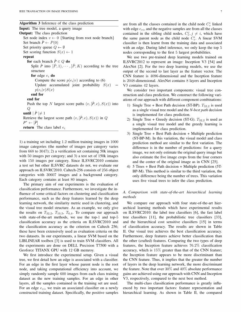
Algorithm 3 Inference of the class predictionInput: The tree model, a query imageOutput: The class prediction

Set node index v ← 0 {Starting from root node branch}Set branch P← P (0)Set priority queue Q← ∅Set scoring function S(x)← 1repeat

for each branch P ∈ Q doSplit P into [P , 1), · · · , [P ,K) according to the treestructurefor edge ei do

Compute the score p(ei|v) according to (6)Update accumulated joint probability S(x) =p(ei|v)S(x)

end forend forPush the top N largest score paths (v, [P, e), S(x)) intoQ

until | P |6= 1Retrieve the largest score path (v, [P, e), S(x)) in QP∗ ← [P]return The class label ei

1) a training set including 1.2 million training images in 1000image categories (the number of images per category variesfrom 668 to 3047); 2) a verification set containing 50k imageswith 50 images per category; and 3) a test set of 150k imageswith 150 images per category. Since ILSVRC2010 containsa test set but other ILSVRC datasets do not, we evaluate ourapproach on ILSVRC2010. Caltech-256 consists of 256 objectcategories with 30607 images and a background category.Each category contains at least 80 images.

The primary aim of our experiments is the evaluation ofclassification performance. Furthermore, we investigate the in-fluence of some critical factors on clustering and classificationperformance, such as the deep features learned by the deeplearning network, the similarity metric used in clustering, andthe visual tree model structure. As an example, we only givethe results on T32,2, T10,3, T6,4. To compare our approachwith state-of-the-art methods, we use the top-1 and top-5classification accuracy as the criteria on ILSVRC2010 andthe classification accuracy as the criterion on Caltech 256;these have been extensively used as evaluation criteria on thetwo datasets. In our experiments, a linear SVM based on theLIBLINEAR toolbox [3] is used to train SVM classifiers. Allthe experiments are done on DELL Precision T7500 with aGeoforce TITANX GPU with 12 GB memroy.

We first introduce the experimental setup. Given a visualtree, we first detail how an edge is associated with a classifier.For an edge in the first layer whose parent node is the rootnode, and taking computational efficiency into account, wesimply randomly sample 600 images from each class trainingdataset as the new training samples. For an edge in otherlayers, all the samples contained in the training set are used.For an edge evi, we train an associated classifier on a newlyconstructed training dataset. Specifically, the positive samples

are from all the classes contained in the child node Civ linked

with edge evi, and the negative samples are from all the classescontained in the sibling child nodes, Cj

v , j 6= i, which havethe same parent node as the child node Ci

v . A linear SVMclassifier is then learnt from the training data and associatedwith an edge. During label inference, we only keep the top 5nodes corresponding to the first 5 largest probabilities.

We use two pre-trained deep learning models trained onILSVRC2012 to represent an image: Inception V3 [54] andAlexNet [2]. For the two deep learning models, we use theoutput of the second to last layer as the feature vector. TheCNN feature is 4096-dimensional and the Inception featureis 2048-dimensional. AlexNet contains 8 layers and InceptionV3 contains 42 layers.

We consider two important components: visual tree con-struction and class prediction. We construct the following vari-ations of our approach with different component combinations:

1) Single Tree + Best Path decision (ST-BP). T32,2 is usedas a single visual tree model and the N-best path decisionis implemented for class prediction.

2) Single Tree + Greedy decision (ST-G). T32,2 is used asa single visual tree model and the greedy learning isimplemented for class prediction.

3) Single Tree + Best Path decision + Multiple prediction(ST-BP-M). In this variation, the visual model and classprediction method are similar to the first variation. Thedifference is in the number of predictions: for a queryimage, we not only estimate the original query image butalso estimate the five image crops from the four cornersand the center of the original image as in CNN [25].

4) 5 Trees + Best Path decision + Multiple prediction (5T-BP-M). This method is similar to the third variation, theonly difference being the number of trees. This variationuses five visual trees to infer the class prediction.

A. Comparison with state-of-the-art hierarchical learningmethods

We compare our approach with four state-of-the-art hier-archical learning methods which have experimental resultson ILSVRC2010: the label tree classifiers [6], the fast labeltree classifiers [11], the probabilistic tree classifiers [33],and the hierarchical cost sensitive classifiers [15] in termsof classification accuracy. The results are shown in TableII. Our visual tree achieves the best classification accuracy.Furthermore, deep features achieve better classification thanthe other (crafted) features. Comparing the two types of deepfeatures, the Inception feature achieves 76.2% classificationaccuracy, which is 15% greater than that of the CNN feature;the Inception feature appears to be more discriminant thanthe CNN feature. Thus, it implies that the greater the numberof layers in the deep learning network, the more discriminantthe feature. Note that over 30% and 40% absolute performancegains are achieved using our approach with CNN and InceptionV3, respectively, compared to the next best method.

The multi-class classification performance is greatly influ-enced by two important factors: feature representation andhierarchical learning. As shown in Table II, the compared


TABLE IICLASSIFICATION ACCURACY (%) COMPARISON ON ILSVRC2010 WITH

DIFFERENT TREE STRUCTURES

T32,2 T10,3 T6,4

Inception3 ST-BP 76.2 74.6 73.6

CNN ST-BP 61.2 60.4 58.7

Hierarchical cost sensitive classifiers [15] 28.3 26.7 24.2

Probabilistic tree classifiers [33] 21.4 20.5 17.0

Label tree classifiers [6] 8.3 6.0 5.9

Fast label tree classifiers [11] 11.9 8.9 5.6

Fig. 4. Comparison of different hierarchical methods on the Inception feature.

hierarchical methods used very different features with eachother. The more distinctive the feature is, the better the classi-fication performance is. In order to investigate the effect of thehierarchical learning, we compare the following hierarchicalmethods under the same feature: the WordNet tree, the labeltree, JDL [62], Relaxed hiearchy [19] and our method. Theyrepresent five typical hierarchical learning methods.

WordNet is a semantic structure according to taxonomywhich is presented on the ImageNet website. We constructa two-layer tree according to the taxonomy distribution of1000 categories of ILSVRC2010. The first-layer nodes arefrom the first-level nodes of WordNet which contains the 1000categories of ILSVRC2010, and all the categories are treatedas the leaf nodes whose hierarchical relations to the first-layernodes agree with the taxonomy. Note that not all the categoriesof ILSVRC2010 are the leaf nodes in WordNet and it is anunbalanced tree. The WordNet tree is denoted as T7,2 whosebranch factor is seven.

Label tree based methods are an important branch of hierar-chical learning methods. Probabilistic tree [33], Label tree [6]and Fast label tree [11] all belong to Label tree based method.We build a simple label tree T32,2 and predict a query imagebased on a greedy learning scheme.

JDL [62] is the latest visual tree constructed based on APclustering. We build a visual tree T32,2 using the Inceptionfeature. JDL is different from other compared methods becauseeach middle node has different feature representation which iscomputed by joint dictionary learning.

Relaxed hiearchy [19] allows each node to neglect theconfusing classes. In other words, a class can be containedin more than one node. This method is only suitable for the

moderate dataset, which is implemented on Caltech 256 andSUN 397 in [19]. When the number of categories becomeslarger, the categories become more confused with each other.And the nodes will grow exponentially which results inprohibited computations. In our experiments, we just constructa shallow binary tree T2,3 using the source code presented bythe authors.

Fig.4 shows the comparison results. Under the conditionsof the Inception feature, our method still achieves the bestresult among different hierarchical methods. The WordNet treeis inferior to our method, which implies that there is a gapbetween the taxonomy and the visual classification. Thus, thetaxonomy structure is not suitable for multi-class visual clas-sification. Moreover, Label tree and Relaxed hierarchy whichused confusing matrix to build a tree are more time consumingthan our method let along their classification accuracies arelower than our method. Our method is superior to JDL [62],and the accuracy difference is 16.43%, because their greedylearning based prediction cannot avoid the error propagation.

B. Comparison with representative state-of-the-art models onILSVRC2010

We next compare our method with seven representativeimage classification methods: HOG+LBP+sparse coding [34],SIFT +Fisher vector [47], Fisher vector [44], one-vs.-all SVM,JDL [62], the hierarchical tree cost sensitivity classifier [15],and the hierarchical tree structure SVM classifier [53]. Thefirst four methods represent the flat classification mechanism,and the last three methods are hierarchical. Moreover, [62] and[15] are greedy learning methods, and [53] and our approachare based on the optimal path searching solution. However,[53] utilizes the structured SVM to solve the class predictionproblem, while our method implements the best path searchto obtain the solution. The one-vs.-all SVM is a popularmethod for multi-class classification. We also treat the one-vs.-all SVM combined with the Inception feature as a benchmarkmethod. A query image is designated to be in a class withthe maximum confidence value. The results are shown inTable III. All the results presented for competing methods arethe original published results; in [62] and [15], the authorsdid not calculate the top-5 results, so these are denoted by”–” (not available). It proves again that the methods usingdeep features outperform the other methods using traditionalfeatures, demonstrating that deep features are more discrimi-native than the traditional features. Furthermore, with the samedeep feature, ST-BP achieve better classification accuracy thanOne-vs.-all+Inception by 1.5%. It implies that our methodcan remarkably improve the classification performance forimbalanced data. In view of the class prediction method, ST-BP is superior to ST-G on CNN features, with an absolutegain of over 5%.

C. Comparison with deep learning network

It is worth noting that CNN [25] was a major milestonein image classification, with many deep learning networksdeveloped thereafter. Inception V3 [54] is one of the latestversions issued by Google Inc. We compare our method with


TABLE IIITHE COMPARISON OF CLASSIFICATION ACCURACY (%) ON ILSVRC2010

Method Top-1 Top-5 Flat Greedy PathSignature + FisherVector [47]

54.3 74.3√

– –

Fisher Vector [44] 45.7 65.9√

– –

HOG + LBP + COD-ING [32]

52.9 71.8√

– –

JDL+AP Clustering[62]

38.9 – –√

–

Hierarchical cost sen-sitivity classifier [15]

41.1 – –√

–

Structured SVM [53] 23.0 – – –√

One-vs.-all+Inception 74.7 90.5√

– –

CNN ST-G 56.1 – –

CNN ST-BP 61.2 81.7 – –√

Inception3 ST-BP 76.2 91.1 – –√

CNN [25]. CNN’s success can be attributed to many factorsthat include a tuned architecture, augmented training data, andensemble decision-making. Inspired by CNN [25], we payparticular attention to the last two factors. In [25], 4 cornerpatches and 1 center patch were cropped and then flipped, so10 images were added to the training data. In our method,we only crop 5 image patches as in [25]. As shown in Table4, our method achieves comparable results to CNN [25]. Thedifference between CNN1 and CNN2 is that CNN1 makes10 predictions for a query image while CNN2 only makes asingle prediction for a query image. Here, we cite the CNNresults given in [25]. Considering the similar decision rule, wecompare ST-BP with CNN2. The top-1 score of our methodis higher than CNN2, while their top-5 scores are similar.With respect to multiple predictions, we use the entire imageand its five crops for class prediction. Comparing ST-BP-Mwith CNN1, even though the augmented training set used inour approach is smaller than in CNN, we achieve comparabletop-1 and top-5 scores to CNN1, and ST-BP-M is superior toCNN2. Comparing 5T-BP-M with CNN1, both use ensembledecision-making, but the size of our augmented data and thenumber of ensemble predictions are smaller than those ofCNN1. The results demonstrate that our method can slightlyoutperform CNN when they are set in a similar environment.Augmented data and ensemble decision-making can improveimage classification performance. Our method is simpler thanCNN [25], because the number of parameters required for ourmethod is much smaller. We also unify the latest Inceptionfeature using our model. Table IV demonstrates that theInception feature achieves the best results compared to othermethods and is more discriminative than the CNN feature. Forboth single and multiple visual trees, the performance of theInception feature is higher by (15%, 9.4%) and (16.5%, 10%)in terms of top-1 and top-5 results, respectively, than theCNN feature. It can also be seen that multiple predictionsprovide even greater gains than ensemble learning. For a singletree with CNN, multiple predictions achieve 0.8% and 0.7%improvements in terms of top-1 and top-5 results, respectively.

TABLE IVCOMPARISON WITH CNN [25] ON ILSVRC2010

Method Top-1 Top-5 Data Augment PredictionCNN1 62.5 83.0 5 crops + flip 10

CNN2 61.0 81.7 5 crops + flip 1

CNN ST-BP 61.2 81.7 no 1

CNN ST-BP-M 62.0 82.4 no 6

CNN 5T-BP-M 62.4 82.7 no 6

Inception3 ST-BP 76.2 91.1 no 1

Inception3 ST-BP-M 77.4 91.8 no 6

Inception3 5T-BP 76.2 90.8 5 crops 1

Inception3 5T-BP-M 78.9 92.4 5 crops 6

Fig. 5. Running time vs. classification accuracy.

Fig. 6. Comparison on average CPU memory cost for a query image.

For multiple trees with Inception features, multiple predictionsachieve 2.7% and 1.6% improvements in terms of top-1 andtop-5 results, respectively.

Furthermore, we discuss the running time and the CPUmemory cost when a query image is tested. We compare thefollowing methods: one-vs.-all SVM, CNN [25], Label treewith the Inception feature, ST-BP CNN and ST-BP Inception.The relation between classification accuracy and the averagerunning time for a query image is shown in Fig.5. The com-parison of CPU memory cost is presented in Fig.6. ComparingCNN [25] with ST-BP CNN and ST-BP Inception, the latter isfaster than CNN, because CNN [25] has to spend more timeon loading the model to the CPU memory while our method,


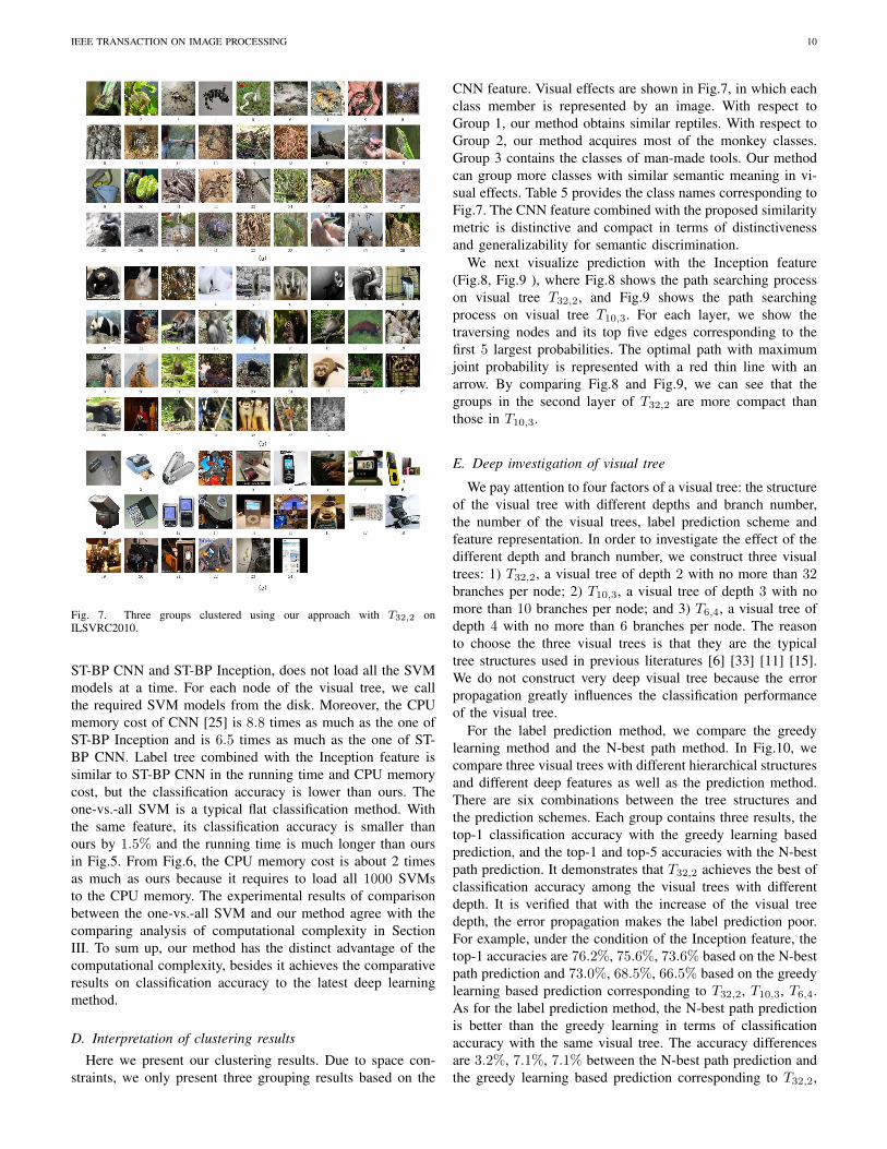
Fig. 7. Three groups clustered using our approach with T32,2 onILSVRC2010.

ST-BP CNN and ST-BP Inception, does not load all the SVMmodels at a time. For each node of the visual tree, we callthe required SVM models from the disk. Moreover, the CPUmemory cost of CNN [25] is 8.8 times as much as the one ofST-BP Inception and is 6.5 times as much as the one of ST-BP CNN. Label tree combined with the Inception feature issimilar to ST-BP CNN in the running time and CPU memorycost, but the classification accuracy is lower than ours. Theone-vs.-all SVM is a typical flat classification method. Withthe same feature, its classification accuracy is smaller thanours by 1.5% and the running time is much longer than oursin Fig.5. From Fig.6, the CPU memory cost is about 2 timesas much as ours because it requires to load all 1000 SVMsto the CPU memory. The experimental results of comparisonbetween the one-vs.-all SVM and our method agree with thecomparing analysis of computational complexity in SectionIII. To sum up, our method has the distinct advantage of thecomputational complexity, besides it achieves the comparativeresults on classification accuracy to the latest deep learningmethod.

D. Interpretation of clustering results

Here we present our clustering results. Due to space con-straints, we only present three grouping results based on the

CNN feature. Visual effects are shown in Fig.7, in which eachclass member is represented by an image. With respect toGroup 1, our method obtains similar reptiles. With respect toGroup 2, our method acquires most of the monkey classes.Group 3 contains the classes of man-made tools. Our methodcan group more classes with similar semantic meaning in vi-sual effects. Table 5 provides the class names corresponding toFig.7. The CNN feature combined with the proposed similaritymetric is distinctive and compact in terms of distinctivenessand generalizability for semantic discrimination.

We next visualize prediction with the Inception feature(Fig.8, Fig.9 ), where Fig.8 shows the path searching processon visual tree T32,2, and Fig.9 shows the path searchingprocess on visual tree T10,3. For each layer, we show thetraversing nodes and its top five edges corresponding to thefirst 5 largest probabilities. The optimal path with maximumjoint probability is represented with a red thin line with anarrow. By comparing Fig.8 and Fig.9, we can see that thegroups in the second layer of T32,2 are more compact thanthose in T10,3.

E. Deep investigation of visual tree

We pay attention to four factors of a visual tree: the structureof the visual tree with different depths and branch number,the number of the visual trees, label prediction scheme andfeature representation. In order to investigate the effect of thedifferent depth and branch number, we construct three visualtrees: 1) T32,2, a visual tree of depth 2 with no more than 32branches per node; 2) T10,3, a visual tree of depth 3 with nomore than 10 branches per node; and 3) T6,4, a visual tree ofdepth 4 with no more than 6 branches per node. The reasonto choose the three visual trees is that they are the typicaltree structures used in previous literatures [6] [33] [11] [15].We do not construct very deep visual tree because the errorpropagation greatly influences the classification performanceof the visual tree.

For the label prediction method, we compare the greedylearning method and the N-best path method. In Fig.10, wecompare three visual trees with different hierarchical structuresand different deep features as well as the prediction method.There are six combinations between the tree structures andthe prediction schemes. Each group contains three results, thetop-1 classification accuracy with the greedy learning basedprediction, and the top-1 and top-5 accuracies with the N-bestpath prediction. It demonstrates that T32,2 achieves the best ofclassification accuracy among the visual trees with differentdepth. It is verified that with the increase of the visual treedepth, the error propagation makes the label prediction poor.For example, under the condition of the Inception feature, thetop-1 accuracies are 76.2%, 75.6%, 73.6% based on the N-bestpath prediction and 73.0%, 68.5%, 66.5% based on the greedylearning based prediction corresponding to T32,2, T10,3, T6,4.As for the label prediction method, the N-best path predictionis better than the greedy learning in terms of classificationaccuracy with the same visual tree. The accuracy differencesare 3.2%, 7.1%, 7.1% between the N-best path prediction andthe greedy learning based prediction corresponding to T32,2,


TABLE VTHE CORRESPONDING CLASS NAMES TO FIG. 7.

Group Class name

a) 1. African chameleon, Chamaeleo chamaeleon 2. American chameleon, anole, Anolis carolinensis 3. European fire salamander, Salamandrasalamandra 4. Gila monster, Heloderma suspectum 5. Indian cobra, Naja naja 6. Komodo dragon, Komodo lizard, dragon lizard, giant lizard,Varanus komodoensis 7. agama 8. alligator lizard 9. banded gecko 10. boa constrictor, Constrictor constrictor 11. box turtle, box tortoise12. bullfrog, Rana catesbeiana 13. common iguana, iguana, Iguana iguana 14. common newt, Triturus vulgaris 15. earthworm, angleworm,fishworm, fishing worm, wiggler, nightwalker, nightcrawler, crawler, dew worm, red worm 16. frilled lizard, Chlamydosaurus kingi 17.garter snake, grass snake 18. green lizard, Lacerta viridis 19. green mamba 20. green snake, grass snake 21. hognose snake, puff adder,sand viper 22. horned viper, cerastes, sand viper, horned asp, Cerastes cornutus 23. king snake, kingsnake 24. leopard frog, spring frog,Rana pipiens 25. millipede, millepede, milliped 26. mud turtle 27. night snake, Hypsiglena torquata 28. ringneck snake, ring-necked snake,ring snake 29. slug 30. tailed frog, bell toad, ribbed toad, tailed toad, Ascaphus trui 31. terrapin 32. thunder snake, worm snake, Carphophisamoenus 33. tree frog, tree-frog 34. vine snake 35. water snake 36. whiptail, whiptail lizard

b) 1. American black bear, black bear, Ursus americanus, Euarctos americanus 2. Angora, Angora rabbit 3. Madagascar cat, ring-tailed lemur,Lemur catta 4. Persian cat 5. baboon 6. badger 7. black-footed ferret, ferret, Mustela nigripes 8. chimpanzee, chimp, Pan troglodytes 9.colobus, colobus monkey 10. giant panda, panda, panda bear, coon bear, Ailuropoda melanoleuca 11. gibbon, Hylobates lar 12. gorilla,Gorilla gorilla 13. guenon, guenon monkey 14. howler monkey, howler 15. indri, indris, Indri indri, Indri brevicaudatus 16. langur 17.lesser panda, red panda, panda, bear cat, cat bear, Ailurus fulgens 18. macaque 19. marmoset 20. meerkat, mierkat 21. mink 22. orangutan,orang, orangutang, Pongo pygmaeus 23. otter 24. patas, hussar monkey, Erythrocebus patas 25. polecat, fitch, foulmart, foumart, Mustelaputorius 26. proboscis monkey, Nasalis larvatus 27. raccoon, racoon 28. siamang, Hylobates syndactylus, Symphalangus syndactylus 29.skunk, polecat, wood pussy 30. sloth bear, Melursus ursinus, Ursus ursinus 31. spider monkey, Ateles geoffroyi 32. squirrel monkey, Saimirisciureus 33. titi, titi monkey 34. weasel

c) 1. CD player 2. Polaroid camera, Polaroid Land camera 3. camcorder 4. carpenter’s kit, tool kit 5. cassette player 6. cellular telephone,cellular phone, cellphone, cell, mobile phone 7. computer keyboard, keypad 8. digital clock 9. flash memory 10. flash, photoflash, flashlamp, flashgun, flashbulb, flash bulb 11. hand calculator, pocket calculator 12. hand-held computer, hand-held microcomputer 13. hard disc,hard disk, fixed disk 14. iPod 15. laptop, laptop computer 16. loudspeaker, speaker, speaker unit, loudspeaker system, speaker system 17.oscilloscope, scope, cathode-ray oscilloscope, CRO 18. point-and-shoot camera 19. projector 20. radio, wireless 21. reflex camera 22. remotecontrol, remote 23. tape player 24. web site, website, internet site, site

Fig. 8. An example of the N-best path search results on the visual tree T32,2 with Inception features on ILSVRC2010.

T10,3, T6,4. Comparing the two deep features, the Inceptionfeature is more distinctive and achieves better classificationperformance than the CNN feature, which is the same as theconclusion made in Subsection A.

We further compare the running time of different hierarchi-cal structures. Fig.11 shows the comparison results. Greedylearning is a little faster than the N-best path method, and thetime differences between them are (21.5ms, 47.5ms, 71.9ms)


Fig. 9. An example of the N-best path search results on the visual tree T10,3 with Inception features on ILSVRC2010.

for the CNN feature, and (22.0ms, 27.2ms, 48.0ms) for theInception feature corresponding to T32,2, T10,3, and T6,4.However, observing Fig.10, the N-best label prediction ismuch better than the greedy learning method on classificationaccuracy.

Furthermore, we have done experiments to investigate theeffect of the different number of visual trees in Fig.12. Withthe increase of the number of the visual tree, the classi-fication accuracy becomes higher, but the increase trend isflat when the number of the visual tree is greater than two.In our experiments, we use five visual trees as the multi-class classification ensemble considering the trade-off betweenclassification accuracy and computational complexity.

Finally, we investigate the effect of different features com-bined with the visual tree T32,2 on classification accuracy. Wecompare four features: SIFT, VLAD, CNN, and Inception V3.SIFT is downloaded from [1], and we use a visual codebookof 1000 visual terms for image representation. For VLAD,we use 256 visual words to form a VLAD feature for imagerepresentation. Since Label Tree [6] uses only simple features,we only compare our approach with Label Tree [6] for faircomparison. Results are shown in Fig.13. Under the conditionof the same feature, our method outperforms Label Tree [6],and our approach can achieve even better performance withmore distinctive deep features, which is the same as the

Fig. 10. Comparison of different visual tree and different label predictionmethods on classification accuracy.

conclusion in Subsection A.

F. Transferring ability

We also compare our method with state-of-the-art methodson visual tree T16,2 on Caltech 256. To compare our methodfairly with other state-of-the-art methods, we use a similarexperimental setup. For each category, we randomly sampleNtrain images as the training data and Ntest images as thetest data. Here, Ntrain = 15, 30, 45 and Ntest = 20, 30, rest,


Fig. 11. Comparison of different visual tree and different label predictionmethods on running time.

Fig. 12. The effect of different number of visual tree on classificationaccuracy.

Fig. 13. Comparison of different features combined with the visual tree T32,2

and the label tree together with SIFT.

where rest means that the remaining samples except thetraining samples are used as test data, since similar parametersettings are considered in the most related works. We run ourmethod three times on Caltech 256 with each combination(Ntrain, Ntest). Three groups of data are randomly generatedfor testing, and the experimental results reported are averagesof these three experiments. Overall, the best path search isbetter than greedy learning in terms of multiple classifications.With an increase in training data, the classification accuracygenerally improves. Fig.14 shows an example of class predic-tion inferred by our method on T16,2 with CNN features.

TABLE VICOMPARISON WITH THE STATE-OF-THE-ART METHODS ON CALTECH 256

IN TERMS OF CLASSIFICATION ACCURACY (%)

MethodFeature

15 30 40 45 50 60

Griffin [23] 28.3 34.1 – – – –

Gemert [21] – 27.2 – – – –

Naveen Kulkarni [27] 39.4 45.8 – 49.3 – 51.4

Yang et al [59] 27.7 34.0 – 37.5 – 40.1

Wang et al [55] 34.4 41.2 – 45.3 – 47.7

CRBM [52] 35.1 42.1 – 45.7 – 47.9

N best path [53] – 35.4 – – – –

Gehler [20] – 45.8 – – 50.8 –

Takumi [26] 40.1 48.6 51.6 – 53.8 –

CNN ST-BP 64.1 68.4 70.1 – – –

Inception3 ST-BP 78.7 81.3 82.5 – – –

TABLE VIITHE COMPARISON OF DIFFERENT DEEP FEATURES IN TERMS OF

CLASSIFICATION ACCURACY (%) ON CALTECH256

Accuracy

Pool5+FV [17] 79.5

CNNs [7] 77.6

ImageNet-CNN [61] 67.2

Hybrid-CNN [61] 65.1

CNN ST-BP 70.1

Inception3 ST-BP 82.5

Comprehensive comparisons are presented in Table VI. Ourapproach achieves the best performance on Caltech 256. Thereasons for this performance improvement are three-fold: 1)deep features are more distinctive for image representationthan traditional feature descriptors such as SIFT; 2) the hier-archical structure is helpful for image classification in additionto the efficiency gain; and 3) our visual tree model - whichcombines visual clustering with object classification - is betterthan the tree model, which only focuses on classification.

We also consider four CNN feature variants: Fisher vectorbased on CNN features [17] (Pool5+FV), CNN pre-trainedon ILSVRC2012 [61] (ImageNet-CNN), CNN trained on thePlaces dataset and Caltech 256 [61] (Hybrid-CNN), and CNNwith accurate networks from the Overfeat package [7](CNNs).We compare the four CNN feature variants with our approach.ImageNet-CNN and hybrid-CNN are similar to our approachand uses a one-vs.-all SVM classifier, while our approachadopts the hierarchical model. The results shown in TableVII suggest that the hierarchical method is superior to theflat classification methods. Furthermore, the deep feature canbe improved if it can be extended with more discriminantfeatures, such as Pool5+FV. CNNs and Inception V3 whichtune the neural network structure improves the classificationperformance, and Inception V3 achieves the best classificationperformance compared to the other CNN features on Caltech256.


Fig. 14. An example of our N-best path search result on Caltech 256. The weight on an edge is the classification confidence.

V. CONCLUSIONS

Here we investigated large-scale object categorization. Weproposed a novel multi-class classification framework basedon hierarchical category structure learning. The aim of ourapproach was to improve the efficiency and accuracy of large-scale object categorization with large numbers of multipleclasses. The core of our approach was to construct a hi-erarchical visual tree and to make class predictions basedon the visual tree model. In particular, we constructed thevisual hierarchical tree using a fast inter-class similarity com-putational algorithm and hierarchical spectral clustering. Wealso proposed an effective path-searching algorithm namedN-best path for class prediction, which was implementedby a joint probability maximization problem. We evaluatedour approach on two large benchmark datasets: ILSVRC2010and Caltech 256. The experimental results demonstrated thatour method is superior to other state-of-the-art hierarchicallearning methods in terms of both the resulting visual treehierarchy and classification accuracy.

VI. ACKNOWLEDGEMENTS

The authors would like to thank editor and anonymous reviewerswho gave valuable suggestions that have helped to improve thequality of the paper. This work was supported by the NationalNatural Science Foundation of China under Grant 61373077, Grant61402480, Grant 61502081, in part by the Hong Kong Scholar Pro-gram, by Australian Research Council under Grant FT-130101457,DP-140102164 and LE-140100061 and by JSPS KAKENHI underGrant 15K16024.

REFERENCES

[1] http://www.image-net.org/.[2] http://caffe.berkeleyvision.org/.[3] http://www.csie.ntu.edu.tw/∼cjlin/liblinear/.[4] S. Bahrampour, N. M. Nasrabadi, A. Ray, and W. K. Jenkins, “Multimodal

task-driven dictionary learning for image classification,” IEEE Trans.Image Processing, vol. 25, no.1, pp. 24-38, 2016.

[5] E. Bart, I. Porteous, P. Perona and M. Welling, “Unsupervised learningof visual taxonomies,” in Proc. IEEE CVPR, June 2008, pp. 1 - 8.

[6] S. Bengio, J. Weston, and D. Grangier, “Label embedding trees for largemulti-class tasks,” In Proc. NIPS, 2010, pp. 163-171.

[7] K. Chatfield, K. Simonyan, A. Vedaldi, and A. Zisserman, “Return ofthe devil in the details: Delving deep into convolutional nets,” In Proc.BMVC, 2014.

[8] C. Chiang, C. H. Liu, C. H. Duan, and S. H. Lai, “Learning component-level sparse representation for image and video categorization,” IEEETrans. Image Process, vol. 22, no. 12, pp. 4775-4787, 2013.

[9] G. Csurka, C. R. Dance, L. Fan, J. Willamowski, and C. Bray, “Visual cat-egorization with bags of keypoints,” In Workshop on Statistical Learningin Computer Vision ECCV, 2004, pp. 1-22.

[10] N. Dalal,and B. Triggs, “Histograms of oriented gradients for humandetection,” In Proc. CVPR, June 2005, pp. 886-893.b

[11] J. Deng, S. Satheesh, A. C. Berg, and F. Li, “Fast and balanced: Efficientlabel tree learning for large scale object recognition,” In Proc. NIPS, 2011,pp. 567-575.

[12] P. Dong, K. Mei, N. Zheng, H. Lei, and J. Fan, “Training inter-relatedclassifiers for automatic image classification and annotation,” PatternRecognition, vol. 46, no. 5, pp. 1382-1395, 2013.

[13] J. Fan, X. He, N. Zhou, J. Peng, and R. Jain, “Quantitative characteri-zation of semantic gaps for learning complexity estimation and inferencemodel selection,” IEEE Trans. Multimedia, vol. 14, no. 5, pp. 1414-1428,2012.

[14] J. Fan, Y. Shen, C. Yang, and N. Zhou, “Structured max-margin learningfor inter-related classifier training and multilabel image annotation,” IEEETrans. Image Process, vol. 20, no. 3, pp. 837-854, 2011.

[15] J. Fan, J. Zhang, K. Mei, J. Peng, and L. Gao, “Cost-sensitive learning ofhierarchical tree classifiers for large-scale image classification and novel

http://www.image-net.org/

http://caffe.berkeleyvision.org/

http://www.csie.ntu.edu.tw/~cjlin/liblinear/


category detection,” Pattern Recognition, vol. 48 no. 5, pp. 1673-1687,2015.

[16] J. Fan, N. Zhou, J. Peng and Y. Gao, “Hierarchical learning of treeclassifiers for large-scale plant species identification,” IEEE Trans. ImageProcess, vol. 24, no. 11, pp. 4172-4184, 2015.

[17] B. Gao, X. Wei, J. Wu, and W. Lin, “Deep Spatial Pyramid: The Devilis Once Again in the Details,” CoRR abs/1504.05277, 2015.

[18] S. Gao, W. Tsang, and Y. Ma, “Learning category-specific dictionaryand shared dictionary for fine-grained image categorization,” IEEE Trans.Image Process, vol.23, no. 2, pp. 623-634, 2014.

[19] T. Gao, and D. Koller, “Discriminative learning of relaxed hierarchyfor large-scale visual recognition,” in Proc. IEEE ICCV, Nov. 2011, pp.2072-2079.

[20] P. Gehler, and S. Novazin, “On feature combination for multiclass objectclassification,” In Proc. IEEE ICCV, Oct. 2009, pp. 221-228.

[21] J. van Gemert, J. Geusebroek, C. Veenman, and A. Smeulders, “Kernelcodebooks for scene categorization,” In Proc. ECCV, 2008, pp. 696-709.

[22] K. Grauman, and T. Darrell, “The pyramid match kernel: Discriminativeclassification with sets of image features,” In Proc. IEEE ICCV, Oct.2005, 1458-1465.

[23] G. Griffin, A. Holub, and P. Perona, “Caltech-256 object categorydataset,” 2007.

[24] G. Griffin, and P. Perona, “Learning and using taxonomies for fast visualcategorization,” in Proc. IEEE CVPR, June 2008, pp. 1 - 8.

[25] A. Krizhevsky, I. Sutskever, and G.E. Hinton, “Imagenet classificationwith deep convolutional neural networks,” In Proc. NIPS, 2012.

[26] T. Kobayashi, “BOF meet HOG: feature extraction based on histogramsof oriented pdf gradients for image classification,” In Proc. IEEE CVPR,June 2013, pp. 747-754.

[27] N. Kulkarni, and B. Li, “Discriminative affine sparse codes for imageclassification,” In Proc. IEEE CVPR, June 2011, pp. 1609-1616.

[28] Y. Lecun, B. Boser, J. S. Denker, D. Henderson, R. E. Howard, H.Hubbard, and L. D. Jackel, “Handwritten digit recognition with a back-propagation network,” In Proc. NIPS, 1997, pp. 396-404.

[29] H. Lei, K. Mei, N. Zheng, P. Dong, N. Zhou, and J. Fan, “Learninggroup-based dictionaries for discriminative image representation,” PatternRecognition, vol. 47, no. 2, pp. 899-913, 2014.

[30] X. Li, X. Zhao, Z. Zhang, F. Wu, Y. Zhuang, J. Wang, and X. Li, “Jointmultilabel classification with vommunity-aware label graph learning,”IEEE Trans. Image Processing, vol. 25, no. 1, pp. 484- 493, 2016.

[31] Y. Li, X. Shi, C. Du, Y. Liu, and Y. Wen “Manifold regularized multi-view feature selection for social image annotation,” Neurocomputing, vol.204, pp. 135-141, 2016.

[32] Y. Lin, F. Lv, S. Zhu, M. Yang, T. Cour, K. Yu, L. Cao, and T.Huang, “Large-scale image classification: Fast feature extraction andSVM training,” In Proc. IEEE CVPR, June 2011, pp. 1689-1696.

[33] B. Liu, F. Sadeghi, M. Tappen, O. Shamir, and C. Liu, “Probabilisticlabel trees for efficient large scale image classification,” in Proc. IEEECVPR, June 2013, pp. 843 - 850.

[34] T. Liu and D. Tao, “Classification with Noisy Labels by ImportanceReweighting”, IEEE Trans. Pattern Anal. Mach. Intell., vol. 38, no. 3,pp. 447-461, March 2016.

[35] D. G. Lowe, “Distinctive image features from scale-invariant keypoints,”International Journal of Computer Vision, vol.60, no. 2, pp. 91-110, 2004.

[36] Y. Luo, D. Tao, K. Ramamohanarao, C. Xu, and Y. Wen, ”TensorCanonical Correlation Analysis for Multi-View Dimension Reduction,”IEEE Trans. Knowl. Data Eng., vol. 27, no. 11, pp. 3111-3124, 2015.

[37] Y. Luo, D. Tao, C. Xu, C. Xu, H. Liu, and Y. Wen, ” Multiview Vector-Valued Manifold Regularization for Multilabel Image Classification,”IEEE Trans. Neural Netw. Learning Syst, vol. 24, no. 5, pp. 709-722,2013.

[38] Y. Luo, Y. Wen, and D. Tao, ”On Combining Side Information andUnlabeled Data for Heterogeneous Multi-task Metric Learning,” In Proc.IJCAI, 2016.

[39] Y. Luo, Y. Wen, D. Tao, J. Gui, and C. Xu, “Large margin multi-modalmulti-task feature extraction for image classification,” IEEE Trans. ImageProcessing, vol. 25, no. 1, pp.414-427, 2016.

[40] M. Marszalek, and C. Schmid, “Constructing category hierarchies forvisual recognition,” In Proc. ECCV, 2008, pp. 479-491.

[41] G. Miller, and C. Fellbaum,“Wordnet: An electronic lexical database,”1998.

[42] A. Y. Ng, M. I. Jordan, and Y. Weiss, “On spectral clustering: Analysisand an algorithm,” In Proc. NIPS, 2002, pp. 849-856.

[43] H. V. Nguyen, H. T. Ho, V. M. Patel, and R. Chellappa, “DASH-N: jointhierarchical domain adaptation and feature learning,” IEEE Trans. ImageProcessing, vol.24, no.12, pp. 5479-5491, 2015.

[44] F. Perronnin, Z. Akata, Z. Harchaoui, and C. Schmid, “Towards goodpractice in large-scale visual image classification,” In Proc. IEEE CVPR,2012, pp. 3482 - 3489.

[45] F. Perronnin, J. Snchez, and T. Mensink, “Improving the fisher kernelfor large-scale image classification,” In Proc. ECCV, 2010, pp. 119-133.

[46] Y. Qu, S. Wu, H. Liu, Y. Xie, and H. Wang, “Evaluation of local featuresand classifiers in BOW model for image classification,” Multimedia Toolsand Applications, vol. 70, pp. 605-624, 2014.

[47] J. Sanchez, and F. Perronnin, “High-dimensional signature compressionfor large-scale image classification,” In Proc. IEEE CVPR, June 2011,pp. 1665-1672.

[48] F. Shen, C. Shen, Q. Shi, A. Hengel, Z. Tang, and H. Shen, “Hashingon Nonlinear Manifolds”, IEEE Trans. Image Processing, vol. 24, no. 6,pp.1839-1851, 2015.

[49] F. Shen, C. Shen, X. Zhou, Y. Yang and H. Shen, “Face ImageClassification by Pooling Raw Features ”, Pattern Recognition, vol. 54,pp.94-103, 2016.

[50] L. Shen, G. Sun, Q. Huang, S. Wang, Z. Lin, and E. Wu, “Multi-leveldiscriminative dictionary learning with application to large scale imageclassification,” IEEE Trans. Image Process, vol. 24, no. 10, pp. 3109-3123, 2015.

[51] J. Sivic, B. C. Russell, A. Zisserman, W. T. Freeman, and A. A. Efros,“Unsupervised discovery of visual object class hierarchies,” in Proc. IEEECVPR, June 2008, pp. 1063-6919.

[52] K. Sohn, D. Jung, H. Lee, and A. O. Hero III, “Efficient learningof sparse, distributed, convolutional feature representations for objectrecognition,” In Proc. IEEE ICCV, Nov. 2011, pp. 2643-2650.

[53] M. Sun, W. Huang, and S. Savarese, “Find the Best Path: An Efficientand Accurate Classifier for Image Hierarchies,” in Proc. IEEE ICCV, Dec.2013, pp. 265-272.

[54] C. Szegedy, V. Vanhoucke, S. Ioffe, J. Shlens, and Z. Wo-jna, “Rethinking the Inception Architecture for Computer Vision,”http://arxiv.org/abs/1512.00567v1.

[55] J. Wang, K. Yu, F. lv, T. Huang, and Y. Gong, “Locality-constrainedlinear coding for image classification,” In Proc. IEEE CVPR, June 2010,pp. 3360-3367.

[56] J. Winn, A. Criminisi, and T. Minka, “Object categorization by learneduniversal visual dictionary,” in Proc. IEEE ICCV, Oct. 2005, pp. 1800-1807.

[57] C. Xu, D. Tao, and C. Xu, “Multi-view Intact Space Learning”, IEEETrans. Pattern Anal. Mach. Intell., vol. 37, no. 12, pp. 2531-2544,December 2015.

[58] C. Xu, D. Tao, and C. Xu,“Large-Margin Multi-view InformationBottleneck”, IEEE Trans. Pattern Anal. Mach. Intell., vol. 36, no. 8, pp.1559-1572, August 2014.

[59] J. Yang, K. Yu, Y. Gong, and T. Huang, “Linear spatial pyramidmatching using sparse coding for image classification,” In Proc. IEEECVPR, June 2009, pp. 1794-1801.

[60] Y. Zhang, J. Wu, and J. Cai, “ Compact representation for imageclassification: To choose or to compress? ” In Proc. IEEE CVPR, June2014, pp. 907-914.

[61] B. Zhou, A. Lapedriza, J. Xiao, A. Torralba, and A. Oliva, “Learningdeep features for scene recognition using places database,” In Proc. NIPS,2014, pp. 487-495.

[62] N. Zhou, and J. Fan, “Jointly learning visually correlated dictionariesfor large-scale visual recognition applications,” IEEE Trans. Pattern Anal.Mach. Intell., vol. 36, no. 4, pp. 715-730, 2014.

[63] X. Zhou, K. Yu, T. zhang, and T. Huang, “Image classification usingsuper-vector coding of local image descriptors,” In Proc. ECCV, 2010,pp. 141-154.

Yanyun Qu received the B.S. and the M.S. degreesin Computational Mathematics from Xiamen Uni-versity and Fudan University, China, in 1995 and1998, respectively, and received the Ph.D. degreesin Automatic Control from Xian Jiaotong University,China, in 2006. She joined the faculty of Departmentof Computer Science in Xiamen University since1998. She was appointed as a lecturer from 2000to 2007 and was appointed as an associate professorsince 2007. Her major research interests include pat-tern recognition and computer vision, with particular

interests in large scale image classification and image restoration. She was atechnology programme chair of ICIMCS2014. She is a member of IEEE andACM.

http://arxiv.org/abs/1512.00567v1


Li Lin received the B.Eng. degree from the De-partment of Computer Science, Xiamen University,in 2014. She is currently working toward the M.S.degree in the Department of Computer Science atXiamen University. Her research interests includeobject detection and recognition.

Fumin Shen received his B.S. and Ph.D. degreefrom Shandong University and Nanjing University ofScience and Technology, China, in 2007 and 2014,respectively. Currently he is an Associate Professorin school of Computer Science and Engineering,University of Electronic of Science and Technologyof China, China. His major research interests includecomputer vision and machine learning, includingface recognition, image analysis, hashing methods,and robust statistics with its applications in computervision. He is a guest editor of Neurocomputing and

a special session organizer of MMM’16.

Chang Lu received the B.Eng. degree from the De-partment of Computer Science, Huanggang NormalUniversity in 2013 and the M.S. degree from XiamenUniversity in 2016. His research interests includeobject detection and recognition.

Yang Wu received a B.S. degree and a Ph.D degreefrom Xi’an Jiaotong University in 2004 and 2010,respectively. From Sep. 2007 to Dec. 2008, he wasa visiting student in the GRASP lab at Universityof Pennsylvania. From 2011 to 2014, he was aprogram specific researcher at the Academic Centerfor Computing and Media Studies, Kyoto University.Within this period, he was an invited academicvisitor at the Big Data Institute of University CollegeLondon from Jul. 2014 to Aug. 2014. He is currentlyan assistant professor of the NAIST International

Collaborative Laboratory for Robotics Vision, Institute for Research Initia-tives, Nara Institute of Science and Technology. His research is in the fieldsof computer vision, pattern recognition, and image/video search and retrieval,with particular interests in detecting, tracking and recognizing humans andgeneric objects. He is also interested in pursuing general data analysis modelsapplicable to large data sets.

Yuan Xie (M’12) received the Ph.D. degree inPattern Recognition and Intelligent Systems fromthe Institute of Automation, Chinese Academy ofSciences (CAS), in 2013. He received his masterdegree in school of Information Science and Tech-nology from Xiamen University, China, in 2010.He is currently with Visual Computing Laboratory,Department of Computing, The Hong Kong Poly-technic University, Kowloon, Hong Kong, and alsowith the Research Center of Precision Sensing andControl, Institute of Automation, CAS. He is the

author of more than research papers, including more than 20 peer-reviewedarticles in international journals such as IEEE Trans. on Image Processing,IEEE Trans. on Neural Network and Learning System, IEEE Trans. onGeoscience and Remote Sensing, IEEE Trans. on Cybernetics, and IEEETrans. on Circuits and Systems for Video Technology. His research interestsinclude image processing, computer vision, machine learning and patternrecognition. He received the Hong Kong Scholar Award from the Society ofHong Kong Scholars and the China National Postdoctoral Council in 2014.

Dacheng Tao (F’15) is Professor of Computer Sci-ence and Director of the Centre for Artificial Intel-ligence, and the Faculty of Engineering and Infor-mation Technology in the University of TechnologySydney. He mainly applies statistics and mathemat-ics to Artificial Intelligence and Data Science. Hisresearch interests spread across computer vision,data science, image processing, machine learning,and video surveillance. His research results haveexpounded in one monograph and 200+ publicationsat prestigious journals and prominent conferences,

such as IEEE T-PAMI, T-NNLS, T-IP, JMLR, IJCV, NIPS, ICML, CVPR,ICCV, ECCV, AISTATS, ICDM; and ACM SIGKDD, with several best paperawards, such as the best theory/algorithm paper runner up award in IEEEICDM07, the best student paper award in IEEE ICDM13, and the 2014 ICDM10-year highest-impact paper award. He received the 2015 Australian Scopus-Eureka Prize, the 2015 ACS Gold Disruptor Award and the 2015 UTS Vice-Chancellors Medal for Exceptional Research. He is a Fellow of the IEEE,OSA, IAPR and SPIE.

ieee transaction on image processing 1 …ieee transaction on image processing 1 joint hierarchical...

Documents