ieee transactions on antennas and ...capolino.eng.uci.edu/publications_papers (local)/othman...ieee...

IEEE TRANSACTIONS ON ANTENNAS AND PROPAGATION, VOL. 65, NO. 10, OCTOBER 2017 5289

Theory of Exceptional Points of Degeneracyin Uniform Coupled Waveguides and

Balance of Gain and LossMohamed A. K. Othman, Student Member, IEEE, and Filippo Capolino, Senior Member, IEEE

Abstract— We present a transmission line theory of exceptionalpoints of degeneracy (EPD) in coupled-mode guiding structures,i.e., a theory that illustrates the characteristics of coupledelectromagnetic modes under a special dispersion degeneracycondition, yet unexplored in the contest of gain and loss. We showthat coupled transmission lines (CTLs) at radio frequencieshaving gain (active devices) and loss (e.g., material, radiation)balance exhibit EPDs. We demonstrate the concept of parity–time (PT )-symmetry in uniform CTLs that involve symmet-ric gain and loss and how this condition is associated witha second-order EPD. Furthermore, we also demonstrate thatPT -symmetry is not a necessary condition for realizing EPDs,and indeed, we show that EPD is also obtained with asymmetricdistributions of gain and loss in uniform CTLs. We furtherpropose potential applications of the EPDs in designing leaky-wave antennas with the capability of beam and directivitycontrol as well as enhanced sensitivity. Operating near suchspecial degeneracy conditions leads to potential performanceenhancement in a variety of microwave and optical resonators,antennas, and devices such as distributed oscillators, includinglasers, amplifiers, radiating oscillators, pulse compressors, andQ-switching sensors.

Index Terms— Antenna design, degeneracies, electromagneticbandgap, multitransmission lines, oscillators, periodic structures,symmetry.

I. INTRODUCTION

ELECTROMAGNETIC propagation eigenvectors in a mul-timodal waveguide may coalesce into a single eigen-

vector when varying frequency or other geometrical/physicalparameters of waveguiding structure; this special point inthe parameter space of the waveguide is called exceptionalpoint of degeneracy (EPD) [1]–[3]. Despite in certain physicsliterature such condition is simply referred to as “EP” thatmay be ambiguous to some other research communities; herewe include a “D” as “degeneracy” in the acronym to specifythe kind of points we are referring to. EPD is associatedwith generalized propagation eigenvectors leading to diverging(growing) waves in space as we will elaborate in the following.

Manuscript received October 30, 2016; revised July 27, 2017; acceptedAugust 2, 2017. Date of publication August 11, 2017; date of current versionOctober 5, 2017. This material is based upon work supported by the AirForce Office of Scientific Research award number FA9550-15-1-0280 andunder the Multidisciplinary University Research Initiative award numberFA9550-12-1-0489 administered through the University of New Mexico.(Corresponding author: Filippo Capolino.)

The authors are with the Department of Electrical Engineering and Com-puter Science, University of California, Irvine, CA 92697 USA (e-mail:[email protected]; [email protected]).

Color versions of one or more of the figures in this paper are availableonline at http://ieeexplore.ieee.org.

Digital Object Identifier 10.1109/TAP.2017.2738063

We investigate EPD conditions of wave propagating eigenvec-tors in coupled transmission lines (CTLs). To avoid ambiguity,the EPD is a different condition than having simple degeneratemodes in waveguides, in which two modes may have thesame eigenvalue (wavenumber) but different field distributions(e.g., two TE11 modes in a circular waveguide with orthogonaltransverse field polarizations). In the latter case, the eigenvalueproblem for finding eigenmodes comprises a diagonalizablesystem matrix; which we will quantify in Section II-A. Notethat the system matrix notion description is ubiquitous foranalyzing the eigenvalues and eigenvectors, also in otherdynamical systems.

On the other hand, EPDs is a degeneracy condition ofeigenvectors of the system and occurs only if the system matrixis non-Hermitian. EPDs are not common but can be found orengineered in many wave guiding structures because they canbe very useful to conceive a variety of devices. The simplestdegeneracy is found at the photonic band edge of periodicstructures, where a regular band edge (RBE) at the edge ofthe Brillouin zone is manifested. The RBE represents a pointat which two Floquet modes with two wavenumbers k and−k + 2π/d coalesce (both in wavenumber and eigenvector)at a single frequency, where d is the period of the periodicstructure [4]–[6]. There, group velocity vanishes in a losslesssystem. Other degeneracies occur at the cutoff frequencyof waveguides [7] or at zero frequency. Periodic structuresin particular can offer interesting degeneracies related tothe electromagnetic bandgap existing in the spectrum ofmodes, which would not be attainable in uniform waveguides.A fourth-order EPD, for instance, occurs when all four inde-pendent Bloch eigenvectors in lossless periodically coupledwaveguides coalesce and form one single eigenvector [4]–[6]at the band edge. This degenerate band edge (DBE) condi-tion is the basis for possible enhancement of gain in activedevices [8], [9], or enhancing directivity in antennas [10], [11]comprising DBE structures. Here instead we discuss moreelaborated and useful degeneracy conditions. The focus of thispaper is on second-order EPDs in waveguides whose wavedynamics are represented by two CTLs with balanced gainand loss. The concept of EPD can also be used to conceivenew low-threshold radio frequency oscillators [12].

The first provided example of such EPD manifestsin guiding structures supporting the so-called parity–time(PT )-symmetric condition [13]–[22], implying that eventhough the system matrix that describes field evolution alongthe CTL is not Hermitian, the system eigenvalues can still bereal [13] when perfect gain and loss symmetric balance is in

0018-926X © 2017 IEEE. Personal use is permitted, but republication/redistribution requires IEEE permission.See http://www.ieee.org/publications_standards/publications/rights/index.html for more information.

5290 IEEE TRANSACTIONS ON ANTENNAS AND PROPAGATION, VOL. 65, NO. 10, OCTOBER 2017

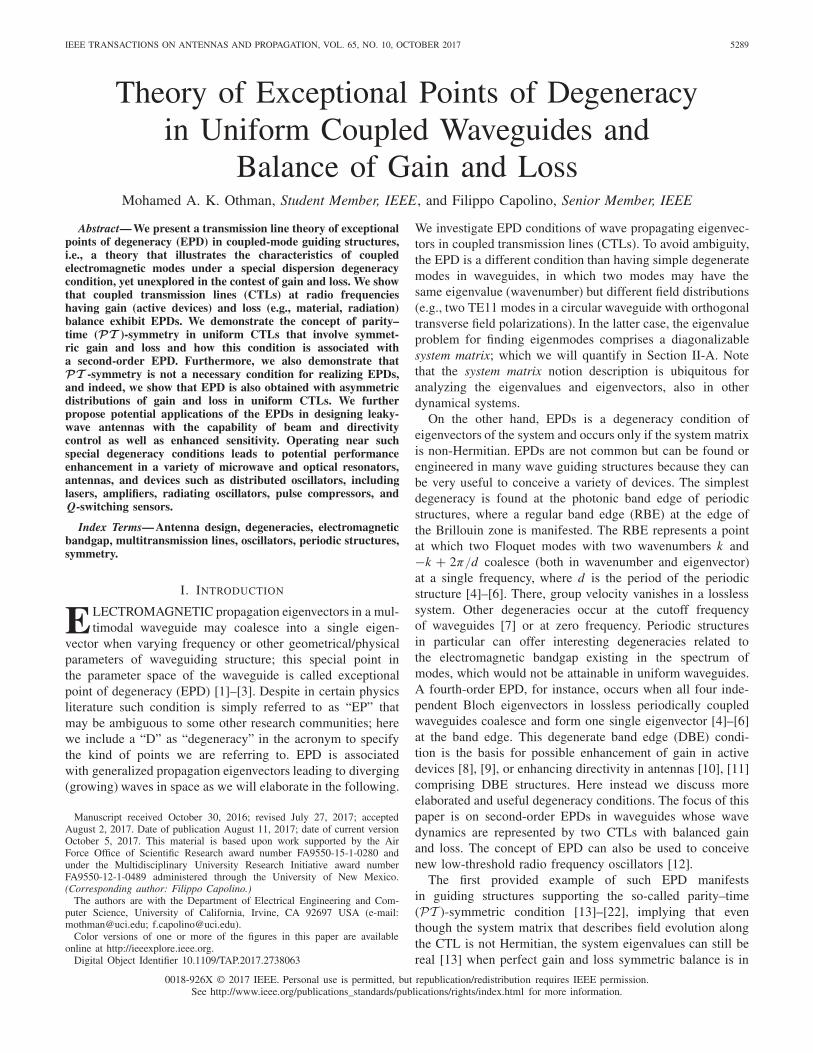
Fig. 1. Example geometries of guided-wave structures that potentiallysupport an EPD in the dispersion diagram. (a) and (b) Coupled waveguidestructures at optical and RF frequencies, respectively, with balanced gainand loss. Waveguides can reach gain and loss balance based on perfectsymmetry (the so-called PT -symmetry condition) as in (a) that leads to asecond-order EPD. The geometry in (b) composed with two lossy and coupledmictrostrips, for example, can satisfy the gain and loss balance condition andhence an EPD without the necessity of symmetric gain and loss (i.e., withoutPT -symmetry). Note that losses could be present mainly due to radiation;the gain is introduced by active devices that can be densely packed (periodis extremely subwavelength) to be approximated as uniformly distributed.

place. (We recall that a sufficient condition for a matrix tohave real eigenvalues is to be Hermitian.) Remarkably, whenthe matrix is not Hermitian, a wide class of non-Hermitiansystem matrices can still possess entirely real spectra. Amongthese are systems obeying PT -symmetry [13]–[22].

Real spectra of non-Hermitian operators (such as thoseobeying PT -symmetry) and the occurrence of EPDs haveopened new horizons on several fronts of physics, includingquantum field theories and quantum interactions [13]. The con-cepts of PT -symmetry have been employed in optics; interest-ing properties have been observed in coupled waveguides andresonators with PT -symmetry when the system’s refractiveindex obeys n(x) = n∗(−x) where x is a coordinate inthe system [15], [17], [23]. By tuning one of the systemvariables, e.g., frequency, gain, and loss parameters, andcoupling, the eigenvalues of a PT -symmetric system tran-sitions from being entirely real valued to be complex, andthe transition point is in fact an EPD [15], [17], [24], [25].In the radio frequency region, there have been some studieson EPDs and PT -symmetry in lumped circuits [26]–[28] andin a microwave cavity [18]. However, a more comprehensiveinvestigation must also be carried out inspired by applicationsand intriguing physics under development in optics.

Note that systems exhibiting only loss (either throughdissipative mechanisms or through via radiation leakage)may also exhibit EPDs [29]. Branches in the eigenmode-frequency dispersion in the context of mode coupling in certainwaveguide geometries have been studied in [7], [30], and [31]and resemble the same near the EPD manifested by balanceof gain and loss discussed here.

In this paper, we develop the theory that reveals the origin ofthe EPDs as well as PT -symmetry in coupled waveguides byadopting a simple CTL model that describes wave propagationin structures such as those in Fig. 1(a) and (b), as examples ofcoupled waveguides with perfect gain and loss compensation.Note that losses need not to be dissipative; in fact, for antennaapplications, losses would naturally represent radiation lossesof antenna elements. The perfect gain and loss distribution inTL1 and TL2, respectively, in Fig. 1 represents what has beenreferred to as PT -symmetry; however, we will show that thisis not a necessary condition to achieve an EPD in practicalterms as we show in this paper. Symmetry of gain and lossof the CTL in this paper is defined as the state when one

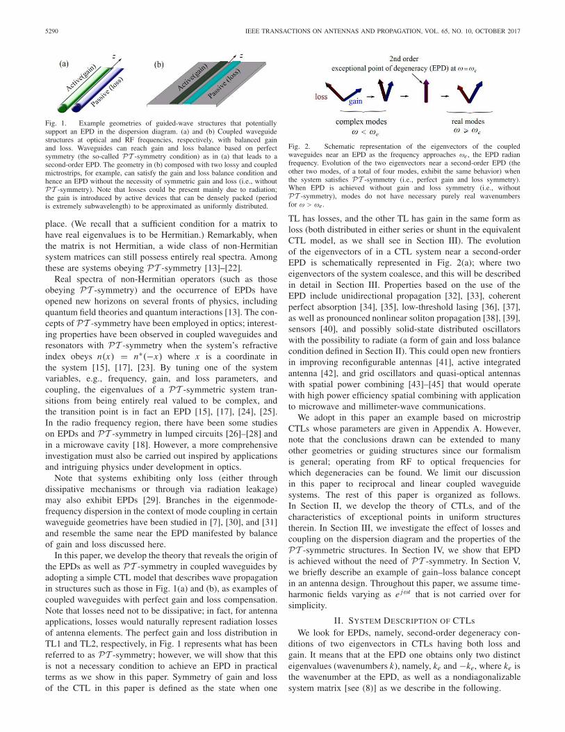
Fig. 2. Schematic representation of the eigenvectors of the coupledwaveguides near an EPD as the frequency approaches ωe, the EPD radianfrequency. Evolution of the two eigenvectors near a second-order EPD (theother two modes, of a total of four modes, exhibit the same behavior) whenthe system satisfies PT -symmetry (i.e., perfect gain and loss symmetry).When EPD is achieved without gain and loss symmetry (i.e., withoutPT -symmetry), modes do not have necessary purely real wavenumbersfor ω > ωe.

TL has losses, and the other TL has gain in the same form asloss (both distributed in either series or shunt in the equivalentCTL model, as we shall see in Section III). The evolutionof the eigenvectors of in a CTL system near a second-orderEPD is schematically represented in Fig. 2(a); where twoeigenvectors of the system coalesce, and this will be describedin detail in Section III. Properties based on the use of theEPD include unidirectional propagation [32], [33], coherentperfect absorption [34], [35], low-threshold lasing [36], [37],as well as pronounced nonlinear soliton propagation [38], [39],sensors [40], and possibly solid-state distributed oscillatorswith the possibility to radiate (a form of gain and loss balancecondition defined in Section II). This could open new frontiersin improving reconfigurable antennas [41], active integratedantenna [42], and grid oscillators and quasi-optical antennaswith spatial power combining [43]–[45] that would operatewith high power efficiency spatial combining with applicationto microwave and millimeter-wave communications.

We adopt in this paper an example based on microstripCTLs whose parameters are given in Appendix A. However,note that the conclusions drawn can be extended to manyother geometries or guiding structures since our formalismis general; operating from RF to optical frequencies forwhich degeneracies can be found. We limit our discussionin this paper to reciprocal and linear coupled waveguidesystems. The rest of this paper is organized as follows.In Section II, we develop the theory of CTLs, and of thecharacteristics of exceptional points in uniform structurestherein. In Section III, we investigate the effect of losses andcoupling on the dispersion diagram and the properties of thePT -symmetric structures. In Section IV, we show that EPDis achieved without the need of PT -symmetry. In Section V,we briefly describe an example of gain–loss balance conceptin an antenna design. Throughout this paper, we assume time-harmonic fields varying as e jωt that is not carried over forsimplicity.

II. SYSTEM DESCRIPTION OF CTLsWe look for EPDs, namely, second-order degeneracy con-

ditions of two eigenvectors in CTLs having both loss andgain. It means that at the EPD one obtains only two distincteigenvalues (wavenumbers k), namely, ke and −ke, where ke isthe wavenumber at the EPD, as well as a nondiagonalizablesystem matrix [see (8)] as we describe in the following.

OTHMAN AND CAPOLINO: THEORY OF EPD UNIFORM COUPLED WAVEGUIDES 5291

Fig. 3. Configurations of CTLs that may exhibit EPD. (a) UniformCTL with distributed and symmetric gain and loss. (b) Uniform CTL withdistributed loss in both TLs and gain in only one. In each case, gain and/orloss can be lumped, but densely enough to be approximated as a uniformdistribution. Moreover, loss could model distributed radiating elements forantenna application.

First, let us consider a waveguide where two modal fieldscoexist and can propagate (as well as possible growth orattenuation) along both the positive and negative z-directions.We seek eigensolutions of the coupled waveguide systemsfound as waves along z. In particular, we look for traditionalsolutions with the z-dependence e− j kz, as well as unconven-tional solutions, present only at the EPD, that behave likeze− j kz as shown in Section II-C. The following procedurecan also describe more than two modes, up to arbitraryN modes. However, here we only focus on two uniformcoupled TLs that pertain to two coupled waveguide structuresas shown in Fig. 1; because to achieve the degeneracy oforder two described here, only two modes (four if we considerthe ±k symmetry, where k is a wavenumber) are sufficient.Waveguides can be unbounded in the transverse to z-direction,and it may be made of uniform [Figs. 1(a) and 3(a)] or quasi-uniform [Fig. 3(b)] that can be approximated as a uniformsystem. (Quasi-uniform means that the structure is spatiallyperiodic, but the period is extremely subwavelength such thatthe coupled waveguide structure can be considered uniformin z, as the case of loading a CTL with densely distributedamplifiers). Let Et (r) and Ht (r) be the transverse componentsof the electric and magnetic fields relative to two modes sup-ported by the uniform waveguide. For simplicity, we assumethat separation of variable in each segment is applicable, andthe transverse electric field is represented as

Et (r) = e1(x, y)V1(z) + e2(x, y)V2(z) (1)

where r = x x+yy+zz. Analogously, we have for the magneticfield

Ht (r) = h1(x, y)I1(z) + h2(x, y)I2(z) (2)

where en(x, y) and hn(x, y), with n = 1,2, are the electric andmagnetic modal eigenfunctions, respectively, and Vn and In arethe amplitudes of those fields that describe the evolution ofelectromagnetic waves along the z-direction (refer to [46] fordescription of the coupled-mode theory and to [47] and [48]for a precise transmission formalism of guided EM wavesin waveguides). We can assume for simplicity that e1(x, y)and e2(x, y) are the orthonormal eigenfunctions. This meansthat they are orthogonal with an inner product defined inthe cross section with a unitary norm, and consequently,the same for h1(x, y) and h2(x, y). This is true for repre-senting uncoupled modes, for example, in waveguides thatare not coupled or far away from each other such that cou-pling is ignored. When waveguides are coupled (for example,

at interfaces of anisotropic materials, or in coupled waveguidegeometries in Fig. 1), fields can still be represented by thoseeigenfunctions, such as the case for even- and odd-fielddistributions for example (e.g., in a coupled microstrip line).In coupled waveguides, we can still define modes that aremutually orthogonal and that, however, consist of equivalentvoltage and current terms along the z-direction. Accordingly,utilizing those eigenfunctions, the guided EM fields can bewell-described by the evolution of their transverse amplitudes(equivalently voltages and currents) resulting in TL equationsthat will be discussed in Section II-A). As a result, for thestructures under consideration as those in Fig. 1, we modelwave propagation along the z-direction for the two modesof interest as CTLs. Therefore, based on (1), and (2) weconsider the amplitudes of the electric and magnetic fieldsas equivalent voltage and current phasor 2-D vectors aredefined as V(z) = [V1(z) V2(z)]T and I(z) = [I1(z) I2(z)]T .Accordingly, the examples in Fig. 1(a) and (b) can be wellrepresented by the respective cases in Fig. 3(a) and (b),respectively, including coupling coefficients per unit length.

A. Uniform Coupled Transmission LinesThe equations for CTLs consisting of two TLs are derived

based on the per-unit-length distributed parameters and usingthe matrix notation [49], [50]. We have the following systemof coupled first-order differential equations representing thefields in uniform transmission lines:

∂V(z)∂z

= −Z I(z),∂I(z)∂z

= −Y V(z) (3)

where Z and Y are the series impedance and shunt admittancematrices describing the per-unit parameters of the CTL definedas

Z = jωL + R, Y = jωC + G (4)

where, for example, the inductance and capacitance are2 × 2 symmetric and positive-definite matrices [49], [50],given in the form

L =(

L11 L12L21 L22

), C =

(C11 C12C21 C22

)(5)

while R and G are the per-unit-length series resistance shuntconductance 2 × 2 matrices, respectively. Both R and Gaccount for losses, and also for small-signal linear gain intro-duced for by negative resistance or conductance. Note thatR and G are positive-definite matrices if and only if theyrepresent only losses [49], [50]. Cutoff conditions could bemodeled by resonant series and shunt reactive elements aswas done in [9] and [51].

To cast the two telegrapher equations in a Cauchy-type first-order partial differential equation, it is convenient to define the4-D state vector

�(z) = [V1(z) V2(z) I1(z) I2(z)]T (6)

that comprises voltages and currents at a coordinate z inthe CTL. Therefore, the first-order differential equations forthe CTL is in written as [5], [9], [51]

∂

∂z�(z) = − jM�(z) (7)


where M is a 4 × 4 CTL system matrix.System Matrix: In a CTL, the system matrix M is given by

M =[

0 − jZ− jY 0

](8)

and 0 is the 2 × 2 zero matrix. We stress that the matrix Mrepresents the system matrix of the CTL and an EPD occurswhen M is not diagonalizable as we illustrate in Section II-C.In the absence of gain and loss, the M matrix satisfies theJ-Hermiticity property [5] (see also [52, Ch. 6]) that is

M† = J M J−1, J = J† = J−1 =[

0 11 0

]

M = −N M N−1, N = N† = N−1 =[

1 00 −1

](9)

where the dagger symbol † denotes the complex conjugatetranspose and 1 is the 2 × 2 identity matrix. The second linein (9) implies that the eigenvalues of M (the wavenumbers)come in positive and negative pairs, as we show in thefollowing.

We first look for solution of (7) of the type �(z) ∝ e− j kz,that is hence rewritten as − jk�(z) = − jM�(z). Hence,eigenmodes supported by the uniform CTL described by (7)are found by solving eigenvalue problem

M�(z) = k�(z) (10)

where k is a wavenumber of the CTL and here it representsthe eigenvalue of the system. When the first equation of (9)holds with a matrix J that is Hermitian and unitary, theeigenvalues (wavenumbers k) of M are real as long as there areno gain and loss. In Appendix B, we also prove, in a differentway, that there is no degeneracy, i.e., M is diagonalizableand has real eigenvalues, in the absence of gain and loss.In Section II-C, we will explore balanced gain and loss andassess the lesser strict condition of PT -symmetry on thematrix M such that an EPD and real-k eigenvalues could befound.

When M is diagonalizable (for example, when M is Her-mitian), one can construct a similarity transformation of Minto a diagonal matrix � containing all the eigenvalues k as

M = U � U−1 (11)

where U is a 4 ×4 matrix, and its column are the four regulareigenvectors �n of M, namely, U = [�1 | �2 | �3 | �4].As such, it is a nonsingular similarity transformation whenit brings M into a diagonal form using (11). Note that suchU becomes singular when M is nondiagonalizable (at the EPD)because at least two eigenvectors coalesce, and hence, theyare no longer independent. (The definitions of a similaritytransformation can be found in [76, Ch. 4. 8] for instance.)

Since M is a 4×4 matrix, (10) has four k-solutions obeyingsymmetric property in reciprocal systems, i.e., ±k are bothsolutions [as indicated from the second unitary transforma-tion in (9)]. Furthermore, we recall that in a lossless CTL,k and k∗ are both solutions. Because of the structure of M,(10) is reduced to two simpler eigenvalue problems of two

dimensions when only eigenvalues are requested. In uniformCTLs, these eigenvalue equations are readily found as

−Z YV(z) = k2V(z), −Y ZI(z) = k2I(z). (12)

Each one provides the four eigenvalues. It is straightforwardto see that in the absence of gain and loss, each of thecharacteristic matrices Z Y or Y Z is similar to a Hermitianmatrix [50], and accordingly, a lossless uniform CTL possessesentirely real-k eigenvalues. A trivial case when the character-istics matrix Z Y or Y Z is non-Hermitian occurs at or below acutoff condition, at which the matrices Z and/or Y become no-longer positive definite as the case of TLs describing TE/TMmodes in rectangular waveguides and their cutoff for instance.Here, we do not investigate cutoff-related degeneracy butrather those special ones occurring when EPD is achieved;i.e., when Z Y or Y Z are not Hermitian at any consideredfrequency, as described in Section III. In general, impedanceand admittance matrices do not commute, i.e., Z Y �= Y Z.A necessary and sufficient condition for these two matricesto commute is that both Z and Y share all of their eigenvec-tors, i.e., they are simultaneously diagonalizable [37], [40].This is obtainable in several kinds of waveguide structures.For example, in lossless multiconductor transmission linesin a homogenous environment [49], [50], the product ofZ Y is given by Z Y = −ω2εμ1; thus, they commute (see[49, Ch. 5]). The commutation property is important whenexamining the characteristics impedance of the system (notinvestigated here for the sake of conciseness). However, ingeneral, Z and Y might not commute, and in the following,we consider this more general case (without resorting to anyparticular assumption rather than they are symmetric; L and Care also positive definite, while R and G are symmetric andrepresent losses and/or gain) as will be further discussed inSection III.

B. Transfer Matrix

Solution of (7), with a certain boundary condition�(z0) = �0 at a certain coordinate z0 inside a uniformCTL segment, is found by representing the state vector solu-tion at a coordinate z1 using

�(z1) = T(z1, z0)�(z0) (13)

where we define T(z1, z0) as the transfer matrix which trans-lates the state vector �(z) between two points z0 and z1 alongthe z axis. Within a uniform segment of a CTL, the transfermatrix is easily calculated as

T(z1, z0) = exp[− j (z1 − z0)M] (14)

and the transfer matrix satisfies the group propertyT(z2, z0) = T(z2, z1)T(z1, z0) as well as the J-unitarity (see[52, Ch. 6 and 9]), that is

T†(z1, z0) = J T−1(z1, z0) J (15)

which is a consequence of reciprocity restriction and J isdefined in (9), in addition to the symmetric propertyT(z1, z0)T(z0, z1) = 1, where 1 is the 4 × 4 identitymatrix (refer to [5] for general properties of the transfermatrix).


C. Exceptional Points of Degeneracy

The EPD is the point in the parameter space of the CTL atwhich M in (8) is not diagonalizable and it is indeed similarto a matrix that contains one or more Jordan blocks. An EPDis associated with repeated eigenvalues, and multiple eigen-vectors coalescing to form a degenerate eigenvector. Recallthat algebraic multiplicity of an eigenvalue is the number it isrepeated in the spectrum of eigenvalues and denoted by m,while the geometric multiplicity is the number of linearlyindependent eigenvectors associated with that eigenvalue, andis denoted by l. (These definitions are found in variouslinear algebra textbook such as in [53, Chs. 6 and 11].)Here, we consider second-order EPDs, which are points inthe spectrum of M when the algebraic multiplicity of theeigenvalues or the wavenumbers m = 2 and their geometricmultiplicity l = 1. Therefore, the system matrix M in (8)cannot be represented as in (11), and M is rather similar to amatrix contain Jordan blocks as

M = W[

�+ 00 �−

]W−1, �+ =

(ke 10 ke

)

�− =( −ke 1

0 −ke

); and

exp (− j�±z) =(

e∓ j kez − jze∓ j kez

0 e∓ j kez

)(16)

implying a second-order degeneracy (see [53, Chs. 6 and 11]).Here, the 4 × 4 matrix W is a nonsingular similarity trans-formation whose columns are two regular eigenvectors andtwo generalized eigenvectors corresponding to wavenumbersolutions ke and −ke, each with multiplicity of two, and�+ and �− in (16) are the 2 × 2 Jordan blocks, i.e., theyare nondiagonalizable. As such, matrix W is written as W =[�1 | �

g1 |�2 | �

g2 ] (see [53, Ch. 6 and 11]) where �1,2 are

the two regular eigenvectors associated with the eigenvalues±ke, respectively, and �

g1,2 are the two generalized eigen-

vectors that are given by �1,2 = (M ∓ ke1)�g1,2 (see [53,

Chs. 6 and 11]). A remarkable feature of a Jordan Block isthat its matrix exponential yields an off-diagonal term that isproportional to ze∓ j kez, as seen in (16) which provides anunusual wave propagation characteristic pertains only to theEPD. A symbolic evolution for one pair of eigenvectors near asecond-order EPD is depicted in Fig. 2 showing they coalescewhen ω = ωe.

The characteristic equations for the eigenvalues of Min (10) can be cast in a simple scalar polynomial of orderfour in k, whose solutions provide the four eigenvalues (i.e.,the wavenumbers). Also from (12), one can write thecharacteristic polynomial for the eigenvalues of a 2 × 2matrix (see [53, p. 14-1]) as

k4 + k2Tr(Z Y) + det(Z Y) = 0 (17)

where Tr and det are the trace and the determinant,respectively, and the analytic expression of eigenvaluesare reported in Appendix B for the special lossless case.In Sections III and IV, we discuss wavenumbers andconditions for EPD occurrence in CTL that incorporates gainand loss with and without PT -symmetry.

III. SECOND-ORDER EPD IN UNIFORM SYMMETRIC CTLsIn this paper, the “gain and loss balance conditions” are

defined as the condition that guarantees the existence of anEPD in such CTL system described in (7). The examplesin Fig. 1(a) and (b) can be well represented by those cor-responding cases in Fig. 3(a) and (b), respectively. Thesetwo cases represent uniform or quasi-uniform waveguides.Results in this section pertain to a uniform guiding systemmade of two identical grounded microstrips in proximity (seeFig. 11 in Appendix A), whose physical parameters are givenin Appendix A as well as its equivalent CTL parameters.Symmetry is defined with respect to a plane containing thez-axis and perpendicular to the plane containing the microstrip.The other example of CTL with asymmetric gain and loss willbe provided in Section IV.

A. Conditions on the CTL Parameters and PT -SymmetryThe identical microstrip coupled lines are described by

a CTL with symmetric and positive definite, per-unit-lengthcapacitance and inductance matrices (5). In the absence ofloss and gain, the system does not develop any EPD except atzero frequency which is a trivial condition. (The proof of thisstatement is detailed in Appendix B.) An EPD at a nonzeroradian frequency, denoted by ωe, is obtained when gain andlosses are introduced, represented here by negative/positiveper-unit-length resistance and/or conductance. We show herethe conditions under which the CTL system matrix M can bewritten in the form (16), thus exhibiting a degenerate modeat ω = ωe.

For simplicity, we assume that the per-unit-length resistanceand conductance matrices are diagonal. In this case, thePT -symmetric condition is equivalent to Z = −� Z† �,Y = −� Y†� when applied to CTLs with gain and loss, and� is the 2 × 2 backward or reverse identity matrix,i.e., with unity antidiagonal elements. This operation sim-ply interchanges the diagonal elements of the per-unit-length impedance and admittance matrices in the presenceof gain/loss. This PT -symmetric condition is the analog ofrefractive index conjugate symmetry often utilized in PT -symmetric optics [17].

Here we consider losses that are introduced as per-unit-length series resistance R2 in TL2, while gain is introducedas per-unit-length negative series resistance R1 in TL1. There-fore, in this example, the series impedance per-unit-lengthmatrix R is diagonal, whereas G = 0. Accordingly, in thiscase, the matrices Z Y and Y Z in (12) are non-Hermitian.Therefore, we consider the gain and loss condition

R2 = −R1 = R (18)

in which we denote R as the distributed gain and lossparameter (real and positive number).

For the CTL under consideration with gain and loss, forsimplicity, we further assume the following symmetries:

C11 = C22 = C, L11 = L22 = L

L12 = L21 = Lm, C12 = C21 = −Cm . (19)

Moreover, the positive-definite condition of the inductance andcapacitance matrices implies L > Lm and C > Cm . When


both (18) and (19) are realized simultaneously for nonzerogain and loss parameter R, we refer to the CTL as beingPT -symmetric. In order that (17) satisfies the second-orderdegeneracy condition at ω = ωe, i.e., (k2 − k2

e )2 = 0, where±ke are the degenerate state eigenvalues, each of multiplicitytwo, the following conditions first must be verified:

Tr(Z Y) = −2k2e , and det(Z Y) = +k4

e . (20)

However, the coincidence of two eigenvalues is not sufficientfor the EPD condition examined in this paper; we also needpairs of eigenvectors to coalesce at radian frequency ωe,associated with each of the two wavenumbers ke and −ke,as schematically represented in Fig. 2. In other words, if atωe we have a degeneracy condition at ke of order two, we alsohave another one at −ke of order two. Therefore, we need to besure that some other necessary condition is also simultaneouslysatisfied. In the particular case of PT-symmetry, we imposethat the Jordan block similarity restriction (16) at ωe and ±ke,leading to a sufficient condition for EPD occurrence [whenthe conditions (18) through (20) are satisfied] that reads[

C2 L2 + C2m L2

m + (C2 − C2

m

) (R

ωe

)2

− (C2 L2

m + C2m L2)

]

= (ke/ωe)4

ω2e [LC − LmCm] = k2

e . (21)

The equations in (21) are found by setting the determinant of U in (11) to equal zero, namely, det(U) = 0, resulting in an equation with complex terms which is casted into two equations with real terms in (21). The conditions in (21) are necessary and sufficient to realize a second-order EPD, under the simplifying PT-symmetry assumptions in (18) and (19). In general one should note that (20) only guarantees eigen-value coincidence for any uniform CTL. However, when the PT-symmetry is enforced from (18) and (19), the conditions in (21) are the same as those obtained from (20) for such particular case. By properly choosing the parameters L, C, and Lm , and a certain Cm = Cm,e, we obtain the value of R that provides for an EPD by imposing (20) and (21) at a desired radian frequency ωe and wavenumber ke.

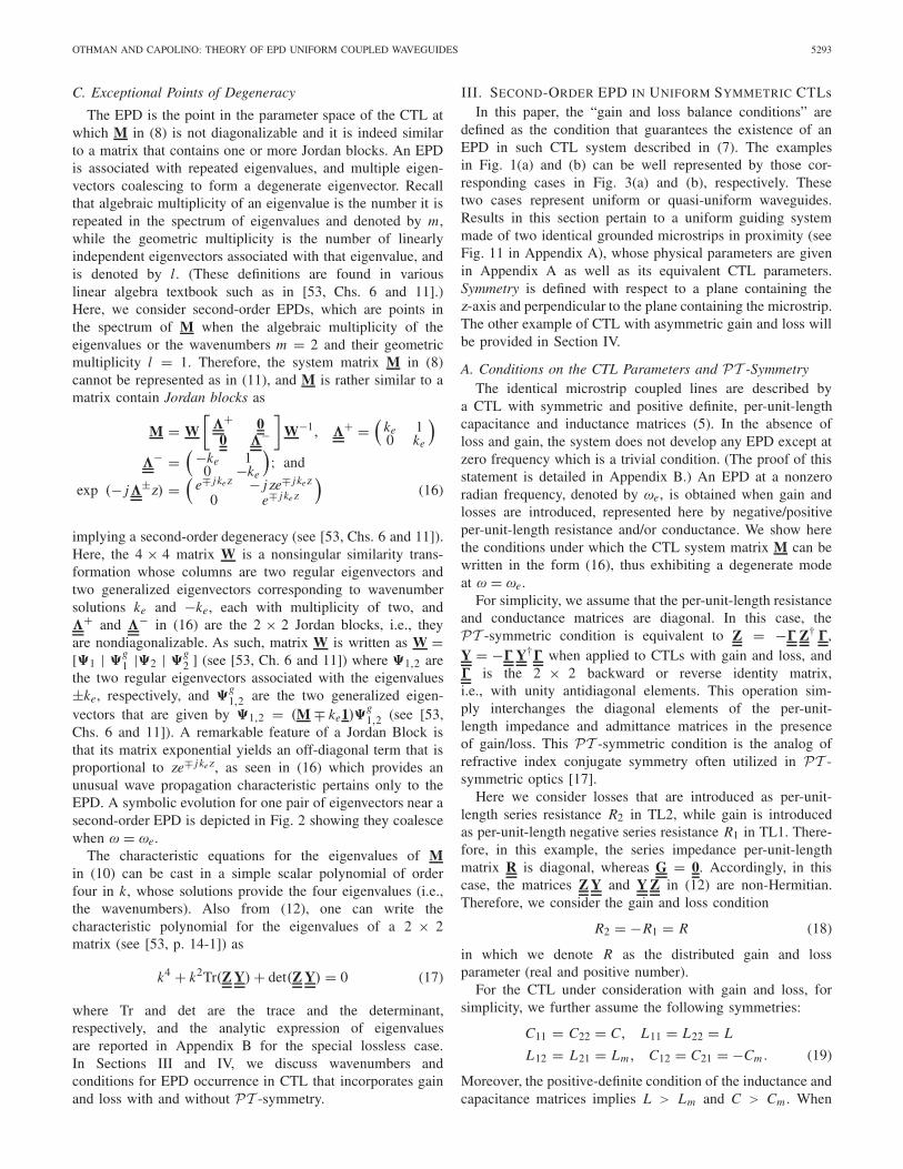
B. Second-Order EPD and PT -SymmetryTo demonstrate the existence of an EPD in a CTL, Fig. 4(a)

shows the dispersion relation of the modes supported bythe CTL system designed to exhibit an EPD at radian fre-quency ωe (i.e., at frequency fe = ωe/(2π) = 1 GHz) andwavenumber ke. The values of the CTL parameters are listed inAppendix A, corresponding to lossy coupled microstrip lineswith distributed amplifiers modeled with distributed negativeresistance. The resulting eigenvalues at the EPD are at bothk = ke and k = −ke, where ke = ωe

√LC − LmCm =

28.66 m−1 as obtained from (21). Note that the dispersiondiagram supports complex modes in general (modes withcomplex wavenumber k for real frequencies), but in Fig. 4(a),we plot only the real part of the wavenumber to show the EPD,at which a bifurcation of modes occurs.

To illustrate that the system has indeed developed an EPDat ω = ωe, we utilize the similarity transformation in (11)

Fig. 4. (a) Dispersion diagram of the wavenumber k versus angularfrequency for a 2-TL with balanced gain–loss; developing an exceptional point(at ω = ωe, k = ke) at which bifurcation of two complex modes intotwo real modes takes place. (b) Magnitude of determinant of the similaritytransformation U in (11). The CTL parameters are given in Appendix A.(c) Complex k space near a second-order EPD. Trajectory of complex k in theRe(k)–Im(k) plane varying as a function of ω. Modes have complex wavenum-ber for ω < ωe (only the real part is shown) and purely real wavenumbers forω > ωe. PT -symmetry occurs for ω = ωe, k = ke where only real modesare observed. (c) Positive branches of the wavenumber evaluated varying asa function of frequency.

that is valid for ω �= ωe and calculate its determinant,namely, |det[U]|, varying as a function of frequency. The|det[U]| measure is used here to identify the occurrence of anyEPD in the system, though it cannot necessarily recover theorder of such degeneracy. Indeed, the 4 ×4 matrix U containsfour independent eigenvectors as columns for any ω �= ωe,but |det[U]| = 0 when at least two eigenvectors coalesce,hence U becomes singular. (We recall that diagonalization ofthe matrix M is a sufficient condition for the existence offour independent eigenvectors, see [53, p. 4-7].) Interestingly,the measure |det[U]| is proportional to the solid angle betweenthe four complex vectors in a 4-D space, and was utilizedin [54] to detect second-order EPDs. This feature is shownin Fig. 4(b) where it is seen that at ω = ωe one has|det[U]| → 0 as an indication that the system is undergoing adegeneracy (of a second order in this case).

In Fig. 4(c), we analyzing the complex Re(k)–Im(k)wavenumber. There the trajectory of the mode’s wavenumberk for two modes with k(ω) and k∗(ω), both with positivereal part, i.e., with phase propagating along the +z-direction,is plotted with increasing angular frequency from 0.5ωe to1.5ωe. The second-order EPD occurs at ωe, at which the twoblue and black curves meet. For frequencies such that ω > ωe,the two wavenumbers are purely real, despite the presence oflosses and gain.


In particular, for the radian frequency lower than theEPD’s ωe, modes are complex with complex conjugatewavenumbers k(ω), k∗(ω),−k(ω),−k∗(ω). Note that k(ω)and k∗(ω) are both solutions in a lossless system; here insteadwith both losses and gain, such symmetry is in principle notnecessarily expected. Indeed, for ω < ωe the right branch ofthe dispersion diagram, with positive Re(k), comprises twomodes, with k(ω) and k∗(ω): one exhibits exponential growthin the positive z-direction, while the other decays exponentiallyin the positive z-direction. The other branch with negativeRe(k) represents also two modes with phase propagation inthe −z-direction that behaves analogously. In this frequencyrange (ω < ωe), modes have complex wavenumbers despiteperfect and symmetrical gain–loss balance. At ωe, pairs ofeigenvalues (wavenumbers) in each branch coalesce at ±ke,hence assuming a vanishing imaginary part and forming twoEPDs, for each of ±ke. For ω > ωe, modes split into pairs withpurely real wavenumber; hence, they do not exhibit neitherexponential growth nor decay, despite the presence of lossand gain. Note that the behavior of the complex wavenumberresembles that around branch points and singularities in thecomplex frequency plane as discussed in [7], [30], and [31].However, the mode bifurcation here is only related to EPDthat is attained through the gain and loss balance.

According to the parameters assumed in the CTL andgoverned by (18) and (19), it is easy to show that the matrixM satisfies the relation M† = � M �−1 where here � is thebackward, also called reverse, identity matrix, i.e., the 4 × 4matrix having ones on the main antidiagonal.

We recall that every complex system with a real spectrumis pseudo-Hermitian [55], i.e., the pseudo-Hermitian systemmatrix can be written as M† = ηMη−1 where η is aHermitian and unitary transformation matrix. (Additionality,if η is also positive-definite, then M has entirely real spec-tra [55]–[57].) Indeed, as shown by Mostafazadeh [55]–[57]all the PT -symmetric Hamiltonians studied in the litera-ture exhibited such property. Note that as described above,we have M† = � M �−1, where � is indeed unitary andHermitian; therefore, the system matrix M in (10) is pseudo-Hermitian. On the one hand, a pseudo-Hermitian matrixpossesses either purely real spectrum or complex conjugatespairs of eigenvalues [55], which is indeed what is depictedin Fig. 4 depending on a system parameter. One the other hand,PT -symmetric strictly is not a necessary nor sufficient condi-tion for a system to develop entirely real spectrum [55]–[57].

To realize such an EPD at a given ωe and ke, a specificamount of gain and loss must be satisfied, as shown inFig. 5 where the gain and loss parameter R is varied at thefixed frequency ω = ωe. Only the positive Re(k) branch isshown for simplicity. Two modes coalesce at a critical valueof the parameter R, denoted by Re. For R < Re, the twomodes are distinct and have purely real wavenumbers. Thecondition R = Re corresponds to the occurrence of the EPDat ω = ωe, and it also designates the onset of “PT -symmetricbreaking” [17], [29].

C. Analysis of EPD PerturbationIt is important to point out that near the second-order

EPD (near in frequency or in some other parameter),

Fig. 5. Positive branches of the wavenumber evaluated at ω = ωe varyingas a function of the gain and loss parameter R. When R reaches a criticalvalue, an EPD is manifested.

Fig. 6. Complex k space near a second-order EPD. Trajectory of complex kin the Re(k)–Im(k) plane varying as a function of Cm , for ω = ωe, where theEPD is manifested at Cm = Cm,e. Note that for symmetry reasons, we haveomitted the −Re(k) branches.

the two eigenvalues of the CTL (i.e., those with positivewavenumbers k) can be written as a small perturbation of thatrelative to the degeneracy condition k = ke, in terms of afractional power expansion as

kn(ω) ∼= ke + anδ1/2 + bnδ + . . . (22)

Analogous discussion is valid near the EPD wavenumber atk = −ke. Here an and bn are the fractional series expansioncoefficients for the two modes in the +z-direction, denotedby n = 1,2, and δ is the small perturbation parameter ofthe system about the EPD (refer to [58] where the para-meters a and b in (22) can be obtained from the system’sexact dispersion relation). In this example, one can assumeδ ≡ (ω −ωe) representing the frequency detuning away fromthe ideal degeneracy frequency, and therefore, (22) representsthe dispersion relation. [The principle square root for δ istaken in (22).] This fractional power expansion, called Puiseuxseries, is a direct consequence of the Jordan Block similar-ity [1], [5], [58], [59]. The branches of dispersion relationin Fig. 4(c) are well fit by (22) in the neighborhood of ω = ωe.

To further elaborate on different perturbation effects in CTL,we inspect how the detuning of some CTL parameter, awayfrom the proper value for which EPD is realized, modifies thedispersion diagram. In Fig. 6, we plot the modal wavenumbers


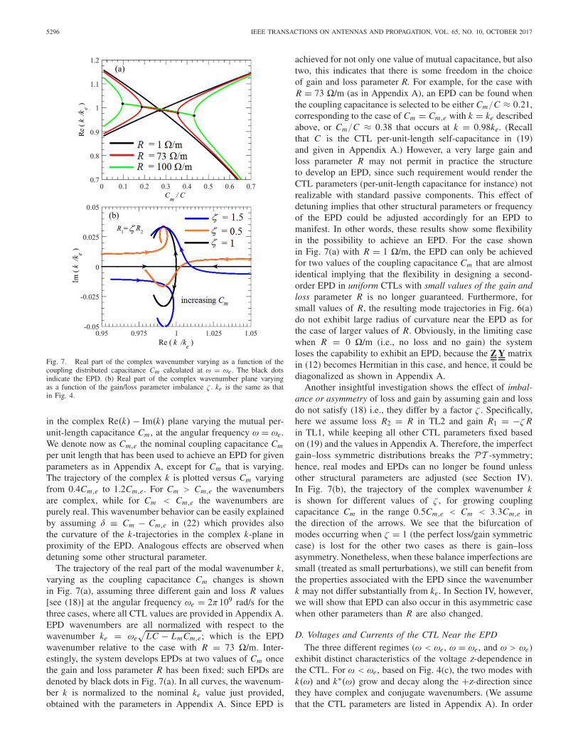
Fig. 7. Real part of the complex wavenumber varying as a function of thecoupling distributed capacitance Cm calculated at ω = ωe. The black dotsindicate the EPD. (b) Real part of the complex wavenumber plane varyingas a function of the gain/loss parameter imbalance ζ . ke is the same as thatin Fig. 4.

in the complex Re(k) − Im(k) plane varying the mutual per-unit-length capacitance Cm , at the angular frequency ω = ωe.We denote now as Cm,e the nominal coupling capacitance Cm

per unit length that has been used to achieve an EPD for givenparameters as in Appendix A, except for Cm that is varying.The trajectory of the complex k is plotted versus Cm varyingfrom 0.4Cm,e to 1.2Cm,e. For Cm > Cm,e the wavenumbersare complex, while for Cm < Cm,e the wavenumbers arepurely real. This wavenumber behavior can be easily explainedby assuming δ ≡ Cm − Cm,e in (22) which provides alsothe curvature of the k-trajectories in the complex k-plane inproximity of the EPD. Analogous effects are observed whendetuning some other structural parameter.

The trajectory of the real part of the modal wavenumber k,varying as the coupling capacitance Cm changes is shownin Fig. 7(a), assuming three different gain and loss R values[see (18)] at the angular frequency ωe = 2π109 rad/s for thethree cases, where all CTL values are provided in Appendix A.EPD wavenumbers are all normalized with respect to thewavenumber ke = ωe

√LC − LmCm,e; which is the EPD

wavenumber relative to the case with R = 73 �/m. Inter-estingly, the system develops EPDs at two values of Cm oncethe gain and loss parameter R has been fixed: such EPDs aredenoted by black dots in Fig. 7(a). In all curves, the wavenum-ber k is normalized to the nominal ke value just provided,obtained with the parameters in Appendix A. Since EPD is

achieved for not only one value of mutual capacitance, but alsotwo, this indicates that there is some freedom in the choiceof gain and loss parameter R. For example, for the case withR = 73 �/m (as in Appendix A), an EPD can be found whenthe coupling capacitance is selected to be either Cm/C ≈ 0.21,corresponding to the case of Cm = Cm,e with k = ke describedabove, or Cm/C ≈ 0.38 that occurs at k = 0.98ke. (Recallthat C is the CTL per-unit-length self-capacitance in (19)and given in Appendix A.) However, a very large gain andloss parameter R may not permit in practice the structureto develop an EPD, since such requirement would render theCTL parameters (per-unit-length capacitance for instance) notrealizable with standard passive components. This effect ofdetuning implies that other structural parameters or frequencyof the EPD could be adjusted accordingly for an EPD tomanifest. In other words, these results show some flexibilityin the possibility to achieve an EPD. For the case shownin Fig. 7(a) with R = 1 �/m, the EPD can only be achievedfor two values of the coupling capacitance Cm that are almostidentical implying that the flexibility in designing a second-order EPD in uniform CTLs with small values of the gain andloss parameter R is no longer guaranteed. Furthermore, forsmall values of R, the resulting mode trajectories in Fig. 6(a)do not exhibit large radius of curvature near the EPD as forthe case of larger values of R. Obviously, in the limiting casewhen R = 0 �/m (i.e., no loss and no gain) the systemloses the capability to exhibit an EPD, because the Z Y matrixin (12) becomes Hermitian in this case, and hence, it could bediagonalized as shown in Appendix A.

Another insightful investigation shows the effect of imbal-ance or asymmetry of loss and gain by assuming gain and lossdo not satisfy (18) i.e., they differ by a factor ζ . Specifically,here we assume loss R2 = R in TL2 and gain R1 = −ζ Rin TL1, while keeping all other CTL parameters fixed basedon (19) and the values in Appendix A. Therefore, the imperfectgain–loss symmetric distributions breaks the PT -symmetry;hence, real modes and EPDs can no longer be found unlessother structural parameters are adjusted (see Section IV).In Fig. 7(b), the trajectory of the complex wavenumber kis shown for different values of ζ , for growing couplingcapacitance Cm in the range 0.5Cm,e < Cm < 3.3Cm,e inthe direction of the arrows. We see that the bifurcation ofmodes occurring when ζ = 1 (the perfect loss/gain symmetriccase) is lost for the other two cases as there is gain–lossasymmetry. Nonetheless, when these balance imperfections aresmall (treated as small perturbations), we still can benefit fromthe properties associated with the EPD since the wavenumberk may not differ substantially from ke. In Section IV, however,we will show that EPD can also occur in this asymmetric casewhen other parameters than R are also changed.

D. Voltages and Currents of the CTL Near the EPDThe three different regimes (ω < ωe, ω = ωe, and ω > ωe)

exhibit distinct characteristics of the voltage z-dependence inthe CTL. For ω < ωe, based on Fig. 4(c), the two modes withk(ω) and k∗(ω) grow and decay along the +z-direction sincethey have complex and conjugate wavenumbers. (We assumethat the CTL parameters are listed in Appendix A). In order


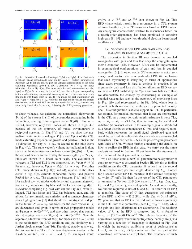
Fig. 8. Behavior of normalized voltages V1(z) and V2(z) of the first modein (a) and (b) and second mode in (c) and (d) in a 2-TL system (parameters inAppendix A). In (a) and (b), we plot the voltages corresponding to the modeexhibiting exponential growth in the +z-direction, for ω < ωe [the modewith blue color in Fig. 4(a)]. The same mode has real wavenumber and alsoV1(z) = V2(z) for ω > ωe. In (c) and (d), we plot voltages correspondingto the mode exhibiting exponential decaying in the +z-direction for ω < ωe(the mode with black color in Fig. 4). The mode has real wavenumber andalso V1(z) = V2(z) for ω > ωe. Note that for each mode voltage and currentdistributions in TL1 and TL2 are not symmetric for ω < ωe, whereas theyare exactly identically for ω > ωe, following the PT -symmetry properties.

to show voltages, we calculate the normalized eigenvectors�n(z) of the system in (10) of the n-modes propagating in thez-direction, starting from a given value �n(0). Here n =1,2,3,4, however, only two modes are shown in Figs. 4–8because of the ±k symmetry of modal wavenumbers inreciprocal systems. In Fig. 8(a) and (b), we show the nor-malized state vector’s voltages V1(z) and V1(z) of the CTLmode exhibiting exponential growth and positive Re(k) in the+z-direction for any ω < ωe, in accord to the blue curvein Fig. 4(c). The state vector’s voltage normalization is donesuch that the state eigenvectors have a norm ‖�n(0)‖ = 1, andthe z-coordinate is normalized by the wavelength λe = 2π/ke.Plots are shown in a linear color scale. The evolution ofvoltages in TL1 and TL2 is not symmetric, i.e., V1(z) �= V2(z)for ω < ωe, however, V1(z) = V2(z) for ω > ωe. The otherCTL mode shown in Fig. 8(c) and (d), relative to the blackcurve in Fig. 4(c), exhibits exponential decay [and positiveRe(k)] for ω < ωe. The asymmetry between V1(z) and V2(z)[for each of the two modes with decay and exponential growthfor ω < ωe, represented by blue and black curves in Fig. 4(c)],is evident comparing Fig. 8(a) with (b) and Fig. 8(c) with (d).Indeed, TL1 has losses and TL2 has balanced gain, and thisallows for asymmetric transmission and resonance character-istics highlighted in [32] that should be investigated in depthin the future. At ω = ωe, solutions for the state vector in (7)are degenerate and given in terms of two propagating modesas �1,2(z) ∝ �(0)e± j kez, and two other modes that containalso diverging terms as �3,4(z) ∝ z�(0)e± j kez. Note thealgebraic z-factor in front of �(0) for modes with n = 3,4 thatis the result from the EPD condition and the similarity to aJordan block as seen from (16). Therefore, exactly at ω = ωe,the voltage in the TLs of the two degenerate modes in the+z-direction (i.e., for n = 1 and 3, for example) would

evolve as e− j kez and ze− j kez (not shown in Fig. 8). ThisEPD characteristic results in a resonance in a CTL systemof finite length, i.e., in a CTL resonator based on EPD modes.An analogous characteristic relative to resonances based ona fourth-order degeneracy has been employed to conceivehigh-gain [8], [9] and new low-threshold electron beam-basedoscillators in [60].

IV. SECOND-ORDER EPD AND GAIN AND LOSS

BALANCE IN UNIFORM ASYMMETRIC CTLs

The discussion in Section III was devoted to coupledwaveguides with gain and loss that obey the conjugate sym-metric condition (18). However, EPDs can be implementedin asymmetrical configurations of gain and loss in coupledwaveguides [61]. In other words, PT -symmetry is not a nec-essary condition to realize a second-order EPD. We emphasizethat such asymmetry is intriguing in terms of applicationssince exact symmetry is hard to achieve in practice. If anasymmetric gain and loss distribution allows an EPD we saywe have an EPD enabled by the “gain and loss balance.” Herewe demonstrate the concept by considering an example ofcoupled waveguides such as the geometry of microstrip linesin Fig. 1(b) and represented as in Fig. 3(b), where loss ispresent in both microstrips, while gain is presented in onlyone. This configuration is able to support an EPD. In particular,we assume, for practical purposes, that losses are representedin the CTL as a series per-unit length resistance in both TLs,R1 = R2 = Re = 73 �/m, thus accounting for metal andradiation (if present) losses. In this example, gain is introducedas a shunt distributed conductance G (real and negative num-ber), which represents the small-signal distributed gain andcould be realized via solid-state devices such as cross-coupledtransistors. Here, we define −G as the positive-gain parameterwith units of S/m. Without further elucidating the details onhow to realize the EPD in this case, we carry out the sameanalysis outlined in Section III yet here for the asymmetricdistribution of shunt gain and series loss.

We also allow some other CTL parameter to be asymmetric;contrary to what was assumed in Section III. We aim at findingconditions on the CTL parameter G as well as the secondTL self-capacitance per unit length, denoted by C22 in orderfor a second-order EPD to manifest at the desired frequencyωe = 2π109 rad/s. We then fix the rest of the CTL parametersas assumed in Section III-B (the values of Rc, L11, L22, Lm ,C11, and Cm that are given in Appendix A), and consequently,we find the required values of G and C22 in order for an EPDto manifest. The value of G that guarantees the existenceof the EPD is G ≈ −83.2 S/m, while C22 ≈ 0.145 nF/m.We point out that an EPD is realized with a minor asymmetryin the CTL intrinsic parameters (here C22/C11 ∼ 1.18), whilethe gain and loss distributions are asymmetric. The resultingvalues of ke at the EPD is complex, and ke is found tobe ke = (28.2 − j0.13) m−1. The relative behavior of thenormalized complex wavenumber trajectory, namely, Re(k/ke)varying as a function of frequency is depicted in Fig. 9(a)in which the trajectory exhibits a point of coalescence atk = ke and ω = ωe. Only curves with the real part of thenormalized wavenumber are plotted. The existence of such


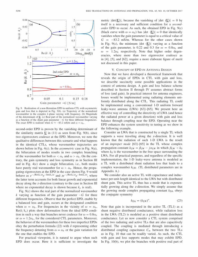
Fig. 9. Realization of a non-Hermitian EPD in uniform CTL with asymmetricgain and loss that is depicted in Fig. 3(b). (a) Trajectory of the normalizedwavenumber in the complex k-plane varying with frequency. (b) Magnitudeof the determinant of U. (c) Real part of the normalized wavenumber varyingas a function of the shunt gain parameter −G for three different frequencies.The exact EPD is realized when G ≈ −83.2 mS/m and ω = ωe.

second-order EPD is proven by the vanishing determinant ofthe similarity matrix U in (11) as seen from Fig. 9(b), sincetwo eigenvectors coalesce at the EPD. Moreover, we note thequalitative differences between this scenario and what happensin the identical CTLs, whose wavenumber trajectories areshown before in Fig. 4(c). In the asymmetric case in Fig. 9(a),the bifurcation of modes results in two complex branchingof the wavenumber for both ω < ωe and ω > ωe. On the con-trary, the gain symmetry and loss symmetry as in Section IIIand in Fig. 4(c) show a single bifurcation, i.e., both modeshave purely real wavenumber for ω > ωe. Hence, the propa-gating eigenvectors at the EPD in the case shown Fig. 9 wouldbehave as e− jRe(ke)ze−Im(ke)z and ze− jRe(ke)ze−Im(ke)z; wherethe latter term accounts for both linear growth and exponentialdecay along the z-direction (contrary to the case in Section IIIwhere no exponential decay is shown because ke is real).

Fig. 9(c) shows the real part of the normalized wavenumberk varying as function of the gain parameter −G for threedifferent frequencies. Observe that the perfect EPD, enable bya balanced loss and gain, occurs at the designated conditionwhen ω = ωe. For frequencies in the vicinity of ω = ωe,Re(k/ke) plots show deformation from the ideal EPD condi-tion in such a way that branches never coalesce for ω = 0.8ωe

or ω = 1.2ωe, for the considered CTL parameters. Moreover,the behavior of the wavenumbers for these two imperfect EPDsobey the perturbation formula (22) with δ representing eitherthe frequency detuning from ω = ωe or the gain variation forthe one that enables the EPD.

For practical viewpoint, it is natural to argue when suchEPD does occur. Here it is sufficient to investigate the

metric |det(U)|, because the vanishing of |det (U)| = 0 byitself is a necessary and sufficient condition for a second-order EPD to occur. As such, the obtained EPD in Fig. 9(c)(black curve with ω = ωe) has |det (U)| = 0 that identicallyvanishes when the gain parameter is equal to a critical value ofG = −83.2 mS/m. Whereas for the other cases shownin Fig. 9(c), the minimum |det (U)| varying as a functionof the gain parameter, is 0.22 and 0.3 for ω = 0.8ωe andω = 1.2ωe respectively. Note that higher order degen-eracies, where more than two eigenvector coalesce asin [4], [5], and [62], require a more elaborate figure of meritnot discussed in this paper.

V. CONCEPT OF EPD IN ANTENNA DESIGN

Now that we have developed a theoretical framework thatreveals the origin of EPDs in CTL with gain and loss,we describe succinctly some possible applications in thecontext of antenna design. A gain and loss balance schemedescribed in Section II through IV assumes abstract formsof loss (and gain). In practical interest for antenna engineers,losses would be implemented using radiating elements uni-formly distributed along the CTL. This radiating TL couldbe implemented using a conventional 1-D uniform forwardleaky-wave antenna (LWA) [63]–[65]. We present here aneffective way of controlling the directivity of LWA (and hencethe radiated power at a given direction) with gain and lossbalance through coupling near the EPD. Operating near theEPD enhances the system sensitivity to tuning as we show inthe following example.

Consider an LWA that is constructed by a single TL whichsupports a wave traveling along the z-direction. It is wellknown that the radiation of such 1-D LWA is the resultof an improper mode [63]–[65] in the TL whose complexpropagation constant kLW = βLW − jαLW in which βLW < k0where k0 is the wavenumber in the free space surrounding theLWA. For all practical purposes, and regardless of the specificimplementation, the 1-D leaky-wave antenna is modeled asa TL with a distributed shunt radiation loss that leads to acomplex wavenumber kLW. (TL distributed parameters are inAppendix A.)

We consider also an active TL with capacitance and induc-tance per-unit-length identical to the LWA but with distributedshunt gain. This active TL thus has a mode that is exponen-tially growing along the z-direction. We simply assume thatthe growing mode complex propagating constant kDA obeysthe conjugate symmetry

kDA = (kLW)∗. (23)

Note that gain is incorporated in the active TL (TL1) as ashunt negative distributed conductance, while radiation lossin the LWA (TL2) is modeled as a positive shunt distributedconductance. Let us now consider a CTL system comprisedof the two radiating and active TLs that are also capacitivelycoupled. The coupling is mediated through introducing adistributed coupling capacitance Cm between the two TLsas in Fig. 10 that can be readily varied. As such, the CTLwith gain and loss supports modes that may exhibit EPD.In Fig. 10(b), we plot the branches with positive real part of


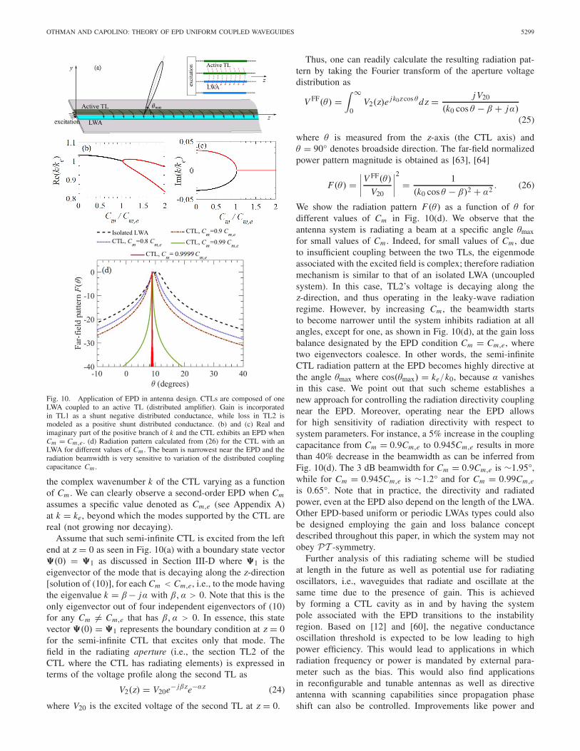
Fig. 10. Application of EPD in antenna design. CTLs are composed of oneLWA coupled to an active TL (distributed amplifier). Gain is incorporatedin TL1 as a shunt negative distributed conductance, while loss in TL2 ismodeled as a positive shunt distributed conductance. (b) and (c) Real andimaginary part of the positive branch of k and the CTL exhibits an EPD whenCm = Cm,e. (d) Radiation pattern calculated from (26) for the CTL with anLWA for different values of Cm . The beam is narrowest near the EPD and theradiation beamwidth is very sensitive to variation of the distributed couplingcapacitance Cm .

the complex wavenumber k of the CTL varying as a functionof Cm . We can clearly observe a second-order EPD when Cm

assumes a specific value denoted as Cm,e (see Appendix A)at k = ke, beyond which the modes supported by the CTL arereal (not growing nor decaying).

Assume that such semi-infinite CTL is excited from the leftend at z = 0 as seen in Fig. 10(a) with a boundary state vector�(0) = �1 as discussed in Section III-D where �1 is theeigenvector of the mode that is decaying along the z-direction[solution of (10)], for each Cm < Cm,e, i.e., to the mode havingthe eigenvalue k = β − jα with β, α > 0. Note that this is theonly eigenvector out of four independent eigenvectors of (10)for any Cm �= Cm,e that has β, α > 0. In essence, this statevector �(0) = �1 represents the boundary condition at z = 0for the semi-infinite CTL that excites only that mode. Thefield in the radiating aperture (i.e., the section TL2 of theCTL where the CTL has radiating elements) is expressed interms of the voltage profile along the second TL as

V2(z) = V20e− jβze−αz (24)

where V20 is the excited voltage of the second TL at z = 0.

Thus, one can readily calculate the resulting radiation pat-tern by taking the Fourier transform of the aperture voltagedistribution as

V FF(θ) =∫ ∞

0V2(z)e

jk0z cos θdz = j V20

(k0 cos θ − β + jα)(25)

where θ is measured from the z-axis (the CTL axis) andθ = 90° denotes broadside direction. The far-field normalizedpower pattern magnitude is obtained as [63], [64]

F(θ) =∣∣∣∣V FF(θ)

V20

∣∣∣∣2

= 1

(k0 cos θ − β)2 + α2 . (26)

We show the radiation pattern F(θ) as a function of θ fordifferent values of Cm in Fig. 10(d). We observe that theantenna system is radiating a beam at a specific angle θmaxfor small values of Cm . Indeed, for small values of Cm , dueto insufficient coupling between the two TLs, the eigenmodeassociated with the excited field is complex; therefore radiationmechanism is similar to that of an isolated LWA (uncoupledsystem). In this case, TL2’s voltage is decaying along thez-direction, and thus operating in the leaky-wave radiationregime. However, by increasing Cm , the beamwidth startsto become narrower until the system inhibits radiation at allangles, except for one, as shown in Fig. 10(d), at the gain lossbalance designated by the EPD condition Cm = Cm,e, wheretwo eigenvectors coalesce. In other words, the semi-infiniteCTL radiation pattern at the EPD becomes highly directive atthe angle θmax where cos(θmax) = ke/k0, because α vanishesin this case. We point out that such scheme establishes anew approach for controlling the radiation directivity couplingnear the EPD. Moreover, operating near the EPD allowsfor high sensitivity of radiation directivity with respect tosystem parameters. For instance, a 5% increase in the couplingcapacitance from Cm = 0.9Cm,e to 0.945Cm,e results in morethan 40% decrease in the beamwidth as can be inferred fromFig. 10(d). The 3 dB beamwidth for Cm = 0.9Cm,e is ∼1.95°,while for Cm = 0.945Cm,e is ∼1.2° and for Cm = 0.99Cm,e

is 0.65°. Note that in practice, the directivity and radiatedpower, even at the EPD also depend on the length of the LWA.Other EPD-based uniform or periodic LWAs types could alsobe designed employing the gain and loss balance conceptdescribed throughout this paper, in which the system may notobey PT -symmetry.

Further analysis of this radiating scheme will be studiedat length in the future as well as potential use for radiatingoscillators, i.e., waveguides that radiate and oscillate at thesame time due to the presence of gain. This is achievedby forming a CTL cavity as in and by having the systempole associated with the EPD transitions to the instabilityregion. Based on [12] and [60], the negative conductanceoscillation threshold is expected to be low leading to highpower efficiency. This would lead to applications in whichradiation frequency or power is mandated by external para-meter such as the bias. This would also find applicationsin reconfigurable and tunable antennas as well as directiveantenna with scanning capabilities since propagation phaseshift can also be controlled. Improvements like power and


radiation efficiency over conventional integrated active antennadesigns, see [42] and references therein, as well as quasi-optical arrays and spatial power combiners [44] that will beinvestigated in a follow-up study.

VI. CONCLUSION

We have demonstrated a transmission line theory ofguided waves in coupled waveguides with EPDs. We haveshown two types of degeneracies that may occur in coupledwaveguides, within the same unified theoretical framework,namely, a second-order EPD in balanced gain–loss uniformwaveguides first satisfying PT -symmetry (i.e., gain and lossdistribution symmetry) and also, importantly, a gain and lossbalance condition without gain and loss symmetry. We havealso developed a figure-of-merit measure for estimating theeffect of imperfect coupling, unbalanced losses and symmetricbreaking on the occurrence of EPDs. In addition, we haveshown an operational principle for LWA based on EPDs whichallows for beamwidth and directivity control through coupling.

The theoretical framework developed here applies to manystructures operating from microwave to optical frequencies andcan readily account for gain provided by the active devices.Because the EPD may be associated with “slow-light” (electro-magnetic wave with vanishing group velocity), extremely highQ-factor resonators can be designed as well high low-thresholdnonlinear processes in the microwave region. An application ofinterest is the balance of gain and loss in high-power travelingwave tubes, promising high efficiency when electron beams actas source of gain while distributed loads represent mechanismof losses or radiation losses. This could be done also in apulse-compression scheme [66] where the electron beam actsalso as a switch. The premise of EPDs would also benefita large category of other applications, such as low-thresholdmicrowave and terahertz sources, antennas, and RF circuits,including radiating array oscillators. Moreover, further investi-gation would be required toward experimentally demonstratingsuch conditions in coupled microstrip transmission lines, as anexample. The EPD may also pave the way to a new schemeof radiating oscillators with advantages like high power effi-ciency, low phase noise, and high power directive generation atmillimeter waves as spatial combiners. Furthermore, inspiredby the extreme sensitivity to one system parameter (couplingin this specific case of Section V) EPD can be used also toconceive a new class of highly sensitive sensors.

APPENDIX ANUMERICAL PARAMETERS USED IN SIMULATIONS

The uniform (i.e., z-invariant) CTL used in this paper cor-responds to two coupled microstrip lines, depicted in Fig. 11and has the following parameters: strip width 3 mm, gapbetween strips 0.1 mm; substrate height 0.75 mm, and dielec-tric constant of 2.2, with a ground plane underneath designedusing Keysight ADS. The corresponding CTL per-unit-lengthparameters are L11 = L22 = L = 0.18 µH/m for both TLs,the mutual inductance is L12 = L21 = Lm = 49.24 nH/m andboth TLs have C11 = C22 = C = 0.12 nF/m, whereas the cou-pling capacitance Cm,e = 25.83 pF/m is chosen to develop asecond-order EPD at 1 GHz, when losses and gain parameters

Fig. 11. Geometry of the microstrip configuration adopted in thispaper (ground plane not shown here). The coupled microstrip lines are madeof two identical metal strips in proximity, and the coupled system developsan EPD when gain and loss are coexisting. On the right, the equivalent CTLis depicted where the red dashed arrows represent coupling and/or powertransfer from the TL with gain to the one without gain.

in (18) are equal to R = 73 �/m, i.e., when R11 = −R22 = Rand R12 = R21 = 0. The value of such distributed series lossresistance in one TL can be achieved using high-loss metaltraces in the microstrip (here Lead can be used whose electricalconductivity is ∼ 4.5 × 106 S/m providing per unit resistancein the microstrip of ∼ 73 �/m when the metal thickness is∼ 10 µm), still being low loss since R < ωL11. It also could beimplemented using a radiating element at its resonance. In theasymmetric case in Section V, we assume losses in both TLssuch as R11 = R22 = R, R12 = R21 = 0, whereas gain isrepresented by the shunt per-unit-length negative conductanceG11 = −G with G22 = G21 = G12 = 0. For the LWAin Section V, we assume that the both radiating and activeTLs have L = 1.6 µH/m, C = 22.7 pF/m, whereas thedistributed radiation loss is characterized by G = 5.5 mS/m,whereas the distributed gain is G = −5.5 mS/m. This leadsto kLW = (kDA)∗ = (0.18 − j0.03)k0 with k0 = ω/c, andthe operational frequency is 1 GHz. The distributed couplingcapacitance at the EPD is found to be Cm,e = 16 pF/m.

APPENDIX BDIAGONALIZATION OF L C AND REAL EIGENVALUES OF

LOSSLESS UNIFORM CTLConsider a lossless, uniform CTL system made by two TLs,

described by its per-unit-length inductance and capacitance2×2 matrices, L and C, respectively. They are strictly symm-etric, and positive-definite matrices following energyconservation requirements [49]; therefore, they possessreal eigenvalues, however in general they are not requiredto commute, i.e., L C �= C L. The four CTL eigenvalues(wavenumbers) are obtained as solutions of the polynomialdet[ω2L C − k21] = 0 or det[ω2C L − k21] = 0, with kbeing the wavenumber. The solution of such eigensystemfor k2(ω) can be written in terms of the inductance andcapacitances matrix entries as assumed in (5) as k2

1,2(ω) =12ω2[(L11C11 + L22C22 − 2LmCm) ± β2], where β4 =[(C11L11−C22L22)

2+4(Cm L11−LmC22)(Cm L22−LmC11)].We shall prove that such lossless CTL never supports

an EPD. Note that if k21(ω) �= k2

2(ω), i.e., there are twodistinct eigenvalues, the associated eigenvectors must be inde-pendent (see [53, Chs. 6 and 11]) and therefore no EPDsexist in this case. However, for the case when k2

1(ω) = k22(ω)

which is necessary condition for an EPD, we will prove thatsuch lossless system (with no loss and no gain) can onlyhave independent eigenvectors when ω > 0, i.e., no EPDexists for any frequency except at zero frequency. It is obvious


that in the special case when L and C commute, the productL C in (12) is symmetric and therefore diagonalizable. Hence,two independent eigenvectors are found and no EPDs occur.Therefore, let us provide a more general proof for the moreinvolved case when L and C do not commute. For the sakeof generality, let us examine whether a matrix Q

vexists

to transform L C into a diagonal matrix � = diag(k21, k2

2)

such that � = Q−1v

L C Qv. In that case, another matrix Q

icould also satisfy � = Q−1

iC L Q

i(recall that a sufficient

condition for matrix diagonalization is the existence of anonsingular similarity transformation such as Q

vor Q

i, see

[53, Chs. 6 and 11]). Now we prove that such matrices (Qi

and Qv) are nonsingular; hence, the matrix L C can be

diagonalized. If it exists, the matrix Qv

is composed of twocolumn eigenvectors, Q

v= [qv1 | qv2] and to prove that

Qvis nonsingular we just need to prove that the two regular

independent eigenvectors qv1,2 exist. To do that we startwriting the eigenvalue problem as ω2L C qv1,2 = k2

1qv1,2 andlook for eigenvalues k2

1,2 and two eigenvectors. The problemcan be rewritten as ω2C qv1,2 = k2

1,2L−1qv1,2, and since Lis symmetric and positive definite, L−1 is also the same.Therefore, since C is also symmetric, and positive definite,the eigenvalues k2

1 and k22 when ω > 0 are always positive and

real for such generalized eigenvalueproblem with symmetric-definite properties ([53, Chs. 15 and 43]). We then proceedwith decomposing L−1 in terms of a lower triangular matrixP as L−1 = P PT ([53, p. 75.9]). Accordingly, the eigenvalueproblem transforms to D zv1,2 = k2

1,2 zv1,2 in which D =ω2P−1C (PT )−1 and zv1,2 = PT qv1,2. Since D is symmetricand real, two eigenvectors zv1,2 exist, and consequently qv1,2are, respectively, linearly independent eigenvectors (see detailsin [53, p. 75.9]). Thus, the matrix Z Y is always diagonalizable(i.e., it cannot exhibit EPDs) in a lossless CTL; even wheneigenvalues are repeated, i.e., when k2

1(ω) = k22(ω). The

special case when k21 = k2

2 = 0 only occurs when ω = 0and yields vanishing eigenvectors which is a trivial scenario.

REFERENCES

[1] T. Kato, Perturbation Theory for Linear Operators, vol. 132. Springer,1995.

[2] W. D. Heiss, “Exceptional points of non-Hermitian operators,” J. Phys.Math. Gen., vol. 37, no. 6, p. 2455, 2004.

[3] W. D. Heiss, “The physics of exceptional points,” J. Phys. Math. Theor.,vol. 45, no. 44, p. 444016, 2012.

[4] A. Figotin and I. Vitebskiy, “Oblique frozen modes in periodic layeredmedia,” Phys. Rev. E, vol. 68, no. 3, p. 036609, Sep. 2003.

[5] A. Figotin and I. Vitebskiy, “Gigantic transmission band-edge resonancein periodic stacks of anisotropic layers,” Phys. Rev. E, vol. 72, no. 3,p. 036619, Sep. 2005.

[6] A. Figotin and I. Vitebskiy, “Frozen light in photonic crystals withdegenerate band edge,” Phys. Rev. E, vol. 74, no. 6, p. 066613,Dec. 2006.

[7] A. B. Yakovlev and G. W. Hanson, “Fundamental modal phenomenaon isotropic and anisotropic planar SLAB dielectric waveguides,” IEEETrans. Antennas Propag., vol. 51, no. 4, pp. 888–897, Apr. 2003.

[8] M. A. K. Othman, F. Yazdi, A. Figotin, and F. Capolino, “Giant gainenhancement in photonic crystals with a degenerate band edge,” Phys.Rev. B, vol. 93, no. 2, p. 024301, 2016.

[9] M. A. K. Othman, M. Veysi, A. Figotin, and F. Capolino, “Giantamplification in degenerate band edge slow-wave structures interactingwith an electron beam,” Phys. Plasmas, vol. 23, no. 3, p. 033112, 2016.

[10] G. Mumcu, K. Sertel, and J. L. Volakis, “Miniature antenna using printedcoupled lines emulating degenerate band edge crystals,” IEEE Trans.Antennas Propag., vol. 57, no. 6, pp. 1618–1624, Jun. 2009.

[11] J. L. Volakis and K. Sertel, “Narrowband and wideband metamaterialantennas based on degenerate band edge and magnetic photonic crys-tals,” Proc. IEEE, vol. 99, no. 10, pp. 1732–1745, Oct. 2011.

[12] D. Oshmarin, F. Yazdi, M. A. K. Othman, M. Radfar, M. Green,and F. Capolino. (Oct. 2016). “Oscillator based on lumped dou-ble ladder circuit with band edge degeneracy.” [Online]. Available:https://arxiv.org/abs/1610.00415

[13] C. M. Bender and S. Boettcher, “Real spectra in non-HermitianHamiltonians having PT symmetry,” Phys. Rev. Lett., vol. 80, p. 5243,Jun. 1998.

[14] W. D. Heiss, M. Müller, and I. Rotter, “Collectivity, phase transitions,and exceptional points in open quantum systems,” Phys. Rev. E, vol. 58,p. 2894, Sep. 1998.

[15] R. El-Ganainy, K. G. Makris, D. N. Christodoulides, andZ. H. Musslimani, “Theory of coupled optical PT -symmetricstructures,” Opt. Lett., vol. 32, no. 17, pp. 2632–2634, 2007.

[16] S. Klaiman, U. Günther, and N. Moiseyev, “Visualization of branchpoints in PT -symmetric waveguides,” Phys. Rev. Lett., vol. 101, no. 8,p. 080402, 2008.

[17] C. E. Rüter, K. G. Makris, R. El-Ganainy, D. N. Christodoulides,M. Segev, and D. Kip, “Observation of parity-time symmetry in optics,”Nature Phys., vol. 6, no. 3, pp. 192–195, 2010.

[18] S. Bittner et al., “PT symmetry and spontaneous symmetry breaking ina microwave billiard,” Phys. Rev. Lett., vol. 108, p. 024101, Jan. 2012.

[19] A. Regensburger, C. Bersch, M.-A. Miri, G. Onishchukov,D. N. Christodoulides, and U. Peschel, “Parity-time synthetic photoniclattices,” Nature, vol. 488, no. 7410, pp. 167–171, 2012.

[20] G. Castaldi, S. Savoia, V. Galdi, A. Alù, and N. Engheta, “PTmetamaterials via complex-coordinate transformation optics,” Phys. Rev.Lett., vol. 110, p. 173901, Apr. 2013.

[21] A. Regensburger et al., “Observation of defect states in PT -symmetricoptical lattices,” Phys. Rev. Lett., vol. 110, no. 22, p. 223902, 2013.

[22] M. Wimmer, A. Regensburger, M.-A. Miri, C. Bersch,D. N. Christodoulides, and U. Peschel, “Observation of opticalsolitons in PT-symmetric lattices,” Nature Commun., vol. 6, Jul. 2015,Art. no. 7782.

[23] I. V. Barashenkov, L. Baker, and N. V. Alexeeva, “PT-symmetry breakingin a necklace of coupled optical waveguides,” Phys. Rev. A, vol. 87, no. 3,p. 033819, 2013.

[24] B. Zhen et al., “Spawning rings of exceptional points out ofDirac cones,” Nature, vol. 525, no. 7569, pp. 354–358, Sep. 2015.

[25] J. Doppler et al., “Dynamically encircling an exceptional point forasymmetric mode switching,” Nature, vol. 537, no. 7618, pp. 76–79,2016.

[26] T. Stehmann, W. D. Heiss, and F. G. Scholtz, “Observation of excep-tional points in electronic circuits,” J. Phys. Math. Gen., vol. 37, no. 31,p. 7813, 2004.

[27] J. Schindler, A. Li, M. C. Zheng, F. M. Ellis, and T. Kottos, “Experi-mental study of active LRC circuits with PT symmetries,” Phys. Rev. A,vol. 84, no. 4, p. 040101, 2011.

[28] M. Chitsazi, S. Factor, J. Schindler, H. Ramezani, F. M. Ellis, andT. Kottos, “Experimental observation of lasing shutdown via asymmetricgain,” Phys. Rev. A, vol. 89, no. 4, p. 043842, 2014.

[29] A. Guo et al., “Observation of PT -symmetry breaking in complexoptical potentials,” Phys. Rev. Lett., vol. 103, no. 9, p. 093902, 2009.

[30] A. B. Yakovlev and G. W. Hanson, “On the nature of critical points inleakage regimes of a conductor-backed coplanar strip line,” IEEE Trans.Microw. Theory Techn., vol. 45, no. 1, pp. 87–94, Jan. 1997.

[31] G. W. Hanson and A. B. Yakovlev, “An analysis of leaky-wave disper-sion phenomena in the vicinity of cutoff using complex frequency planesingularities,” Radio Sci., vol. 33, no. 4, pp. 803–819, Apr. 1998.

[32] H. Ramezani, T. Kottos, R. El-Ganainy, and D. N. Christodoulides, “Uni-directional nonlinear PT -symmetric optical structures,” Phys. Rev. A,vol. 82, no. 4, p. 043803, 2010.

[33] Z. Lin, H. Ramezani, T. Eichelkraut, T. Kottos, H. Cao, andD. N. Christodoulides, “Unidirectional invisibility induced byPT -symmetric periodic structures,” Phys. Rev. Lett., vol. 106, no. 21,p. 213901, 2011.

[34] Y. D. Chong, L. Ge, H. Cao, and A. D. Stone, “Coherent perfectabsorbers: Time-reversed lasers,” Phys. Rev. Lett., vol. 105, no. 5,p. 053901, 2010.

[35] S. Longhi, “PT -symmetric laser absorber,” Phys. Rev. A, vol. 82, no. 3,p. 031801, 2010.


[36] M. Kulishov and B. Kress, “Distributed Bragg reflector structures basedon PT -symmetric coupling with lowest possible lasing threshold,” Opt.Exp., vol. 21, no. 19, pp. 22327–22337, 2013.

[37] L. Feng, Z. J. Wong, R.-M. Ma, Y. Wang, and X. Zhang, “Single-modelaser by parity-time symmetry breaking,” Science, vol. 346, no. 6212,pp. 972–975, 2014.

[38] F. K. Abdullaev, Y. V. Kartashov, V. V. Konotop, and D. A. Zezyulin,“Solitons in PT-symmetric nonlinear lattices,” Phys. Rev. A, vol. 83,no. 4, p. 041805, 2011.

[39] V. V. Konotop, J. Yang, and D. Zezyulin, “Nonlinear waves inPT -symmetric systems,” Rev. Modern Phys., vol. 88, no. 3, p. 035002,2016.

[40] J. Wiersig, “Sensors operating at exceptional points: General theory,”Phys. Rev. A, vol. 93, no. 3, p. 033809, 2016.

[41] J. Costantinea, Y. Tawkb, Y. Barbin, and C. Christodoulou, “Reconfig-urable antennas: Design and applications,” Proc. IEEE, vol. 103, no. 3,pp. 424–437, Mar. 2015.

[42] K. Chang, R. A. York, P. S. Hall, and T. Itoh, “Active integratedantennas,” IEEE Trans. Microw. Theory Techn., vol. 50, no. 3,pp. 937–944, Mar. 2002.

[43] Z. B. Popovic and D. B. Rutledge, “Diode-grid oscillators,” in Proc.IEEE Antennas Propag. Soc. Int. Symp., New York, NY, USA, Feb. 1988,pp. 442–445.

[44] R. A. York and Z. B. Popovic, Active and Quasi-Optical Arrays forSolid-State Power Combining, vol. 42. Hoboken, NJ, USA: Wiley, 1997.

[45] M. P. DeLisio and R. A. York, “Quasi-optical and spatial powercombining,” IEEE Trans. Microw. Theory Techn., vol. 50, no. 3,pp. 929–936, Mar. 2002.

[46] A. Yariv, “Coupled-mode theory for guided-wave optics,” IEEE J.Quantum Electron., vol. 9, no. 9, pp. 919–933, Sep. 1973.

[47] N. Marcuvitz and J. Schwinger, “On the representation of the electricand magnetic fields produced by currents and discontinuities in waveguides. I,” J. Appl. Phys., vol. 22, no. 6, pp. 806–819, Jun. 1951.

[48] L. B. Felsen and N. Marcuvitz, Radiation and Scattering of Waves.Hoboken, NJ, USA: Wiley, 1994.

[49] C. R. Paul, Analysis of Multiconductor Transmission Lines. Hoboken,NJ, USA: Wiley, 2008.

[50] G. Miano and A. Maffucci, Transmission Lines and Lumped Circuits:Fundamentals and Applications. San Francisco, CA, USA: Academic,2001.

[51] M. Othman, V. A. Tamma, and F. Capolino, “Theory and new ampli-fication regime in periodic multi modal slow wave structures withdegeneracy interacting with an electron beam,” IEEE Trans. PlasmaSci., vol. 44, no. 4, pp. 594–611, Apr. 2016.

[52] K. Veselic, Damped Oscillations of Linear Systems: A MathematicalIntroduction, vol. 2023. Berlin, Germany: Springer-Verlag, 2011.

[53] L. Hogben, Handbook of Linear Algebra. Boca Raton, FL, USA:CRC Press, 2006.

[54] M. C. Zheng, D. N. Christodoulides, R. Fleischmann, and T. Kottos,“PT optical lattices and universality in beam dynamics,” Phys. Rev. A,vol. 82, no. 1, p. 010103, 2010.

[55] A. Mostafazadeh, “Pseudo-Hermiticity versus PT symmetry: The nec-essary condition for the reality of the spectrum of a non-HermitianHamiltonian,” J. Math. Phys., vol. 43, no. 1, pp. 205–214, 2002.

[56] A. Mostafazadeh, “Pseudo-Hermiticity versus PT -symmetry: II.A complete characterization of non-Hermitian Hamiltonians with a realspectrum,” J. Math. Phys., vol. 43, no. 5, pp. 2814–2816, 2002.

[57] A. Mostafazadeh, “Pseudo-Hermiticity versus PT -Symmetry III: Equiv-alence of pseudo-Her miticity and the presence of antilinear symme-tries,” J. Math. Phys., vol. 43, no. 8, pp. 3944–3951, 2002.

[58] A. Welters, “On explicit recursive formulas in the spectral perturbationanalysis of a Jordan block,” SIAM J. Matrix Anal. Appl., vol. 32, no. 1,pp. 1–22, 2011.

[59] A. Figotin and I. Vitebskiy, “Slow light in photonic crystals,” WavesRandom Complex Media, vol. 16, no. 3, pp. 293–382, 2006.

[60] M. A. Othman, M. Veysi, A. Figotin, and F. Capolino, “Low startingelectron beam current in degenerate band edge oscillators,” IEEE TransPlasma Sci, vol. 44, no. 6, pp. 918–929, Jun. 2016.

[61] S. N. Ghosh and Y. D. Chong, “Exceptional points and asymmetricmode conversion in quasi-guided dual-mode optical waveguides,” Sci.Rep., vol. 6, p. 19837, Apr. 2016.

[62] J. Sloan, M. Othman, and F. Capolino. (Aug. 2016). “Theory of doubleladder lumped circuits with degenerate band edge.” [Online]. Available:https://arxiv.org/abs/1609.00044

[63] A. A. Oliner and D. R. Jackson, “Leaky-wave antennas,” in AntennaEngineering Handbook, vol. 4. J. L. Volakis, Ed. New York, NY, USA:McGraw-Hill, 2007, ch. 11.

[64] D. R. Jackson and A. A. Oliner, “Leaky-wave antennas,” in ModernAntenna Handbook, C. A. Balanis, Ed. New York, NY, USA: Wiley,2008, ch. 7.

[65] D. R. Jackson, C. Caloz, and T. Itoh, “Leaky-wave antennas,” Proc.IEEE, vol. 100, no. 7, pp. 2194–2206, Jul. 2012.

[66] V. A. Tamma, A. Figotin, and F. Capolino, “Concept for pulse compres-sion device using structured spatial energy distribution,” IEEE Trans.Microw. Theory Techn., vol. 64, no. 3, pp. 742–755, Mar. 2016.

Mohamed A. K. Othman (S’10) received the B.S.and M.S. degrees in electrical engineering fromCairo University, Cairo, Egypt, in 2009 and 2012,respectively. He is currently pursuing the Ph.D.degree with the Department of Electrical Engineer-ing and Computer Science, University of California,Irvine, CA, USA.

In 2013, he joined Institut d’électronique demicroélectronique et de nanotechnologie, Lille,France, as a Visiting student. In 2015 and 2016,he was a Research Student with the Technology

Innovation Directorate, SLAC National Accelerator Laboratory, Menlo Park,CA, USA. His current research interests include high-power microwave gen-eration, dispersion engineering, RF bandgap circuits and oscillators, graphene-based photonics, RF accelerator cavity and driver amplifier design, andnumerical methods including eigenmode projection techniques and FDTD,metamaterials, and plasmonics.

Filippo Capolino (S’94–M’97–SM’04) receivedthe Laurea (cum laude) and Ph.D. degrees in elec-trical engineering from the University of Florence,Florence, Italy, in 1993 and 1997, respectively.

He has been an Assistant Professor at the Depart-ment of Information Engineering, University ofSiena, Siena, Italy. From 1997 to 1999, he was aFulbright and then a Postdoctoral Fellow with theDepartment of Aerospace and Mechanical Engineer-ing, Boston University, MA, USA. From 2000 to2001, part of 2005 and in 2006, he was a Research

Assistant Visiting Professor with the Department of Electrical and Com-puter Engineering, University of Houston, TX, USA. He was a short-termVisiting Professor at the Fresnel Institute, Marseille, France, in 2003, andat the Center de Recherche Paul Pascal, Bordeaux, France, in 2010. He iscurrently a Full Professor with the Department of Electrical Engineering andComputer Science, University of California, Irvine, CA, USA. His currentresearch interests include metamaterials and their applications, traveling wavetubes, oscillators, antennas, sensors in both microwave and optical ranges,plasmonics, microscopy, wireless systems, millimeter waves, chip-integratedantennas and applied electromagnetics in general.

Dr. Capolino was the EU Coordinator of the EU Doctoral Programs onMetamaterials from 2004 to 2009. He received the R. W. P. King Prize PaperAward from the IEEE Antennas and Propagation Society for the Best Paperof the Year 2000, by an author under 36. From 2002 to 2008, he servedas an Associate Editor of the IEEE TRANSACTIONS ON ANTENNAS AND

PROPAGATION. He is the Editor of the Metamaterials Handbook (Boca Raton,FL, USA: CRC Press, 2009).

ieee transactions on antennas and ...capolino.eng.uci.edu/publications_papers (local)/othman...ieee...

Documents