ieee transactions on circuits and systems-i: … · 2019-08-16 · ing paradigm for pattern...

IEEE TRANSACTIONS ON CIRCUITS AND SYSTEMS-I: FUNDAMENTAL THEORY AND APPLICATIONS, VOL. 42, NO. 10, OCTOBER 1995 559

Autonomous Cellular Neural Networks: A Unified Paradigm for Pattern

Formation and Active Wave Propagation Leon 0. Chua, Fellow, IEEE, Martin Hasler, Fellow, IEEE, George S. Moschytz, Fellow, IEEE,

and Jacques Neirynck, Fellow, IEEE

Abstract-This tutorial paper proposes a subclass of cellular neural networks (CNN) having no inputs (i.e., autonomous) as a universal active substrate or medium for modeling and generating many pattern formation and nonlinear wave phenomena from numerous disciplines, including biology, chemistry, ecology, engineering, physics, etc. Each CNN is defined mathematically by its cell dynamics (e.g., state equations) and synaptic law, which specifies each cell’s interaction with its neighbors. We focus in this paper on reaction4iffusion CNNs having a linear synaptic law that approximates a spatial Laplacian operator. Such a synaptic law can be realized by one or more layers of linear resistor couplings.

An autonomous CNN made of third-order universal cells and coupled to each other by only one layer of linear resistors provides a unified active medium for generating trigger (autowave) waves, target (concentric) waves, spiral waves, and scroll waves. When a second layer of linear resistors is added to couple a second capacitor voltage in each cell to its neighboring cells, the resulting CNN can be used to generate various turingpatterns. Although the equations describing these autonomous CNNs represent an excel- lent approximation to the nonlinear partial differential equations describing reaction-diffusion systems if the number of cells is sufficiently large, they can exhibit new phenomena (e.g., propagation failure) that can not be obtained from their limiting partial differential equations. This demonstrates that the autonomous CNN is in some sense more general than its associated nonlinear partial differential equations.

To demonstrate how an autonomous CNN can serve as a unifying paradigm for pattern formation and active wave propagation, several well-known examples chosen from different disciplines are mapped into a generic reaction-diffusion CNN made of third- order cells.

Finally, several examples that can not be modeled by reaction-diffusion equations are mapped into other classes of autonomous CNNs in order to illustrate the universality of the CNN paradigm.

I. INTRODUCTION

S INCE ITS inception in 1988 [l], cellular neural networks (CNNs) have been widely studied for both static and dy-

namic image processing applications [2]-[ lo]. In these applications, the input u(t) to the CNN at any time t is usually a gray-scale image, coded as a capacitor voltage at each cell

Manuscript received December 18, 1994; revised June 12, 1995. This paper was recomended by Guest Editor L. 0. Chua.

L. 0. Chua is with the Department of Electrical Engineering and Computer Science, University of California at Berkeley, Berkeley, CA 94720 USA.

M. Hasler and J. Neirynck are with the Ecole Politechnique Federale de Lausanne, Switzerland.

G. S. Moschytz is with the Swiss Federale Institute of Technology at Zurich, Ztirich, Switzerland.

IEEE Log Number 9414452.

n;j at location (ij) in a Cartesian coordinate system.’ The output image in this case is caused directly by the input image. In this paper, we propose to use the CNN for an entirely different class of applications where no external input image is applied, and where the output image at any time t is due exclusively to initial conditions. The initial conditions can be a random field, (e.g., for Turing pattern formation), a noisy image (e.g., a blurred finger print), an incomplete image (e.g., for associative memory), etc. The corresponding output will be a desired pattern, a sharpened image, ‘a reconstructed picture, etc.

In this paper, the terms “patterns” and “waves” will.be used in their broadest possible context. In particular, a “pattern” can be a still image, or a recurrent image (e.g., a nonlinear standing wave), and a “wave” can be a traveling pulse (e.g., a soliton) or pulse train, a trigger wave, a target (concentric) wave, a spiral wave, a scroll wave, or even a chaotic wave, etc. These phenomena, though still poorly understood at this point in time, are universal and robust in the sense that they have been observed and reported from almost every scientific and social disciplines (e.g., astronomy, biology, chemistry, demography, ecology, economics, engineering, . . . physics, . . . , zoology). Our goal in this paper is to demonstrate how a subclass of autonomous cellular neural networks can provide a unifying paradigm for explaining and controlling these fascinating phenomena from so many diverse disciplines whose only common denominator is the ubiquitous nonlinearity endowed upon them.

II. CELLULAR NEURAL NETWORKS: A FORMAL MATHEMATICAL DEFINITION

A cellular neural network (CNN) is a high-dimensional dynamic nonlinear circuit having a mainly locally-recurrent circuit topology; namely, a local interconnection of simple circuit units called cells, or artificial neurons. The resulting net or array may have any architecture, including rectangular, hexagonal, toroidal, spherical, etc. In this tutorial paper, we will consider only a rectangular array for simplicity.

In most applications, all cells and their interconnections are assumed to be identical although the original concept of a CNN given in [l] includes the possibility of variable interconnections and circuit parameters. The key concept that

‘We use the term cell to mean an artificial neuron in this paper.

1057-7122/95$04.00 0 1995 IEEE

560 IEEE TRANSACTIONS ON CIRCUITS AND SYSTEMS-I: FUNDAMENTAL THEORY AND APPLICATIONS, VOL. 42, NO. 10, OCTOBER 1995

m (i+lJ+l)

Fig. 1. A CNN cell rz;j (bottom) located at site (ij) in a rectangular architecture and its synaptic input current I& consisting of contributions from the states ~;+k,~+l of its neighbor cells, shown for a sphere of influence S;j consisting of only eight nearest neighbors (middle section) and from the inputs

u;+k,j+l of its neighbor cells (top). The weighting coefficients akl and bkl can be any nonlinear functions of the state variables, may contain time delays, and may vary with location. For the usual space-invariant CNN, all cells are identical, i.e., ak(,bkl do not depend on ij.

distinguishes a CNN from other neural networks is that the interconnections among cells be mainly2 local in order to minimize the chip area occupied by connecting wires. To simplify our notation in this paper, however, we will assume all cells and their interconnections to be identical. In addition, we will consider only one-, and two-dimensional CNN arrays even though most concepts on CNNs are applicable to any dimension n > 3 as well. In view of these assumptions, it suffices for us to examine only one cell and its interconnection circuitry with the neighboring cells, as shown in Fig. 1.

The basic CNN cell nij shown at the bottom of Fig. 1 contains in addition to the dynamical circuit core characterized by its state vector xij, an input Wij, a threshold (dc bias) Zij, an output yij, and a synaptic input current I$. This synaptic current depends on the input Ui+k,j+l (t) and the state zi+k,j+l(t) of all cells located within a prescribed sphere ofin- $uence S$, or neighborhood size, which in this paper consists simply of the eight nearest neighboring cells. The contribution from the input Ui+k,j+l(t) of each neighbor cell ni+k,j+l E Sij is modeled by a linear controlled source bklUi+k,j+l, as shown in the upper part of Fig. 1. The contribution from the

‘The term “mainly” is used to allow the possibility of global coarse graining (e.g., the addition of global controlling wires in the CNN universal machine [2]-[3]), an important feature found in higher brain functions [4].

state x;+k,j+l(t) of each neighbor cell ni+k,j+l is modeled by a nonlinear controlled source aklf(~i+k,j+l), where f(.) is a prescribed nonlinear scalar function of xi+k,j+l(t), as depicted in the middle part of Fig. 1. In this figure, the synaptic input current I&(t) is uniquely specified by only 16 synaptic coe@cients akl and bkl associated with the eight nearest neighbors of cell nij. These coefficients are usually listed as entries (along with two nonsynaptic coefficients a00 and boo) of the following two tables, generally referred to as the feedback template A and feedforward (input) template B, respectively:

piE$qmi’

Template A Template B

The central coefficients a00 of template A and boo of template B pertain to the corresponding feedback and feedforward contributions inside the cell n;j itself in the original first- order CNN cell proposed in [l]. To emphasize that they are independent of the neighboring cells, we have separated them from the eight “synaptic” controlled current sources in Fig. 1. Although the self-feedback coefficient aaa pertains to circuitry inside the cell proper in Fig. 1, it is singled out and included in the A template with the other synaptic coefficients (which is external to the cell nij) because it is sometimes useful to use aaa as a controlling or bifurcation parameter [l], as in Fig. 3(a), or to combine it with the synaptic circuitry to achieve a simpler circuit realization of certain classes of CNNs (e.g., Fig. 5, the reaction-diffusion CNN in Section IV).

The synaptic input current I$(t) shown entering the cell n;j in Fig. 1 accounts for the contributions of all neighbor cells lying within the prescribed sphere of influence S;j of cell nij. These contributions are analogous to the inputs from the “dendrites” of biological neurons. In such neurons, the “synapse” is used to convert the electrical signal coming from the output (axon) of a neighbor neuron into a “chemical” signal. In other words, the synapse in a biological neuron can be interpreted as a nonlinear controlled source, as depicted in the middle part of Fig. 1, except that in a real neuron, there are thousands of such controlled sources, working at a relatively slow time scale (milliseconds). In the current generation of CNN chips, there are only eight controlled sources; but they are at least a million times faster, i.e., in nanoseconds. The key idea of the CNN universal chip [2]-[3] is to trade the extremely high speed of VLSI chips with the enormous number of biological synapses in our modest attempt to mimic rudimentary brain functions.

Fig. 1 shows only the simplest case where each synaptic controlled source is controlled by only one state variable of a neighboring cell, as in the original CNN cell proposed in [l]. In the most general case, each synaptic controlled source may depend on several state variables from a neighbor cell (characterized by higher-order dynamics). In addition, the coefficients akl and bkl may be nonlinearfunctionals of not only the neighbor states xi+k,j+l and inputs &+k,j+l, but also

CHUA et al.: AUTONOMOUS CELLULAR NEURAL NETWORKS 561

A (i+l,j+l)

A template

al,-1 %,o ai ,I EEI ao.-1 ao.0 a0,1

a-~,-i a-1,0 a-l,1

1; 25 ?t “ii

Site (id)

N

+ Yij

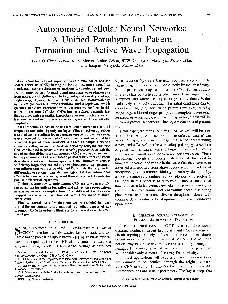
Fig. 2. An autonomous CNN cell does not have external inputs (Wj =w+!%,j+1 = 0). Each synaptic controlled current source is shown here as a nonlinear function of its present state z;~ and its neighbor state z;+k,j+l for each ICZ E S;j. The synaptic coefficients akl are listed in an A template.

possibly its own state xij and input ~;j.~ For example, akl f(‘) may be any mathematical operation (e.g., nonlinear delay operator, convolution operator, Volterra series operator, etc.) on the internal state Xij(t) and its neighbor state Si+k,j+l(t). To emphasize this generalization, we introduce an asterisk “*” between akl and f(.), as shown in Fig. 2. Some examples of operators that can significantly increase the processing power of the CNN are

1) akl * f(si+k,j+l(t),zij(t)) = aklf(%+k,j+l(t - T)

- xij (t - T)) t

2) akl * f(xi+k,j+l(t),xij(t)) = akl J’

qt - T) 0

3) akl * f(%+k,j+l(t)) = akl where xij 2 vZZ3 ; uij & Eij; and I& is the synaptic input current defined by

.h,(t-Tl,t-T2 )...) t-7,)

’ %+k,j+1(71) ’ ’ .X;+k,j+l(Tn) dT1 h-2. . . dT,.

The internal circuit core of each cell nij in Fig. 1 can be any dynamical system defined by an evolution equation, or even a semigroup in the most abstract version. In this paper, nij will be made of lumped circuit elements and hence its dynamics is simply described by its associated state equations. For example, in the simplest class of CNN proposed in [l], the basic cell reproduced and shown in Fig. 3(a) is described by the following first-order state equation:

IzYj = C aklf(Xi+k,j+l) + C bkl’G+k,j+l (2.2) klES,, klESij kZ#O,O kl#O,O

and f(.) is the only nonlinearity defined by

f(x) 2 $ [Ix + 11 - Ix - 111. (2.3)

In this paper, aJirst-order cell nij is characterized by

aoof(xij) - boouij - I - If’ 1 (2.1)

“uij “Xii “Yij

(a)

(b) 1; /

+ iR

:il

+ c xij “R

-I- T

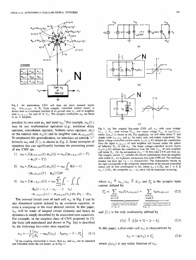
Cc) Fig. 3. (a) The original first-order CNN cell n;j with input voltage Vu%3 = Eij, state voltage Vz%3, and ourprrt voltage Vu%, = a~~of(z,,), where f(~,~) is shown in (b). For simplicity, we will often delete V and simply write u;j, zij, and yzj for input, state, and output, respectively. The linear voltage-controlled current source I,, (i, j; kl) denotes the contribution from the input u;+k,j+l of each neighbor cell located within the sphere of influence S;j of cell n,j. The linear voltage-controlled current source I,,(i, j; LX’) denotes the contribution from the state V,,, of each neighbor cell inside S;j. (b) An autonomous (u;j = 0) first-order CNN cell from (a). The synaptic current I:? includes all current contributions from the neighbor cells within S;j. (c) A generic autonomous first-order CNN cell. The nonlinear resistor can have any 21~ - in characteristic. The characteristic shown on the right corresponds to the composite characteristic of the resistor-controlled source and dc bias combination in (b), where uz3 > l/RI and I = 0. If at3 < l/R,, the composite VR - in curve will be monotone increasing.

ki;ij = -g(Xij) + I.fj (2.4) 31f the coupling relationship is linear, then z;j and uij can be separated

and imbedded inside the cell proper, as in Fig. 1. where g(xij) is any scalar function of xij.


For a general (not necessarily space-invariant or isotropic) CNN whose cells are made of time-invariant circuit elements, each cell nij is characterized by its4 CNN cell dynamics where

xcu E R” and z,, 1~~ are usually scalars. In most cases, the interactions (spatial coupling) with the neighbor cells ni+k,j+r are specified by a CNN synaptic law: where the repeated index

,0 is to be interpreted (analogous to the standard Einstein notation in physics) as a summation of contributions from each neighbor cell n,+p located within the prescribed sphere of influence S, about n,. In this paper, S, will usually include only the 8 nearest neighbors, although most concepts and results on CNN are applicable-mutatis mutandis-to a sphere S, of any size, including the extreme case where each cell is connected to all other cells (fully-connected case). In the equations below S, will also denote the index set of the neighborhood, i.e., for the eight nearest neighbor case, kl E S, H k,l E {-l,O,l},(k,Z) # (0,O).

The first term atxcu+p in (2.6) is simply a linearfeedback of the states of the neighboring nodes n,+o, and can be written in the following explicit form:

(2.7)

The second term At * fp(xa,xa+p) in (2.6) provides an arbitrary nonlinear coupling, including infinite-dimensional functional operators, between neighboring cells. In the original CNN cell proposed in [I], this coupling is nonlinear but memoryless; namely

A: * fp(Xa,Xa+p) = c @ij,kZf(xi+k,j+l). (2.8) LlES,

Observe’that the first spatial coupling term aEx,+p in (2.6) can be considered as .a special case of the second spatial coupling term-hence the reason for ,using the same letter A for both terms. However, since there are many examples of CNNs [ 1 l]-[ 171 where only a linear spatial coupling is used, it is convenient to introduce it in (2.6) as a separate contribution. In the usual case where the second nonlinear coupling term in (2.6) is absent, we will often use Ai instead of at.

The third term Bi * ua+p(t) in (2.6) accounts for the contributions from the external inputs of each neighbor cell that is located within S,, where again in the most general

4We will often denote the index ij by Q and kl by p for simplicity.

case * can be any functional or operator. In most cases of interests, we have simply

B,p * %+~(t) = c bij,kl%+k,j+l. (2.9) k1ES.a

In more general cases, &j,kl, &j&, and bij,kl can be matrices. We conclude this section by summarizing the following

formal mathematical definition of a cellular neural network: An N x N cellular neural network is defined mathematically

by four specifications:

41 3) Boundary conditions (see Section IV-A);

For analytical investigations, it is often necessary to assume an autonomous CNN of injinite size, i.e., N -+ co. In this case, the boundary conditions are replaced by the prescribed behavior of the solution at .infinity.

We will assume space invariance or isotropy which means that the coefficients &j&l and &j,kl are independent of ij and will be denoted henceforth as iLkl and ukl, similarly with &j,kl and bij,kl.

III. AUTONOMOUS CELLULAR NEURAL NETWORKS In this paper, we assume .that there are no inputs, i.e.,

~~ij(t) = 0 so that the basic CNN unit of Fig. 1 reduces to that shown in Fig. 2, where for the sake of generality, the synaptic contribution @ lf(xi+k,j+l) in Fig. 1 is replaced by the operator akl * f(ti+k,j+l, zij) introduced earlier. We will henceforth refer to this zero-input CNN as an autonomous cellular neural network. Unless otherwise stated, we will choose the output variables of each cell to be some internal state variable, i.e., r&(t) = ~$(t), k = 1,2, . . . m, where x$(t) denotes the kth component of the state vector xij(t). Because of this trivial identity, the output terminal yij in cell nij of Fig. 1 will usually be deleted.

A. Some Generic Autonomous CNN Cells

Stripping the input Eij and coupling term I,,(i, j; kl) from the neighboring inputs from Fig. 3(a), and grouping all coupling terms &(i, j; 51) from all neighbor cells n.;+k,j+l, kl E S, (kl # 0,O) into the synaptic input current I$, we obtain the simplified CNN cell shown in Fig. 3(b). Observe that the nonlinear controlled source aaaf(x~j) across the output resistor R, in Fig. 3(a) with (k, 1) = (0,O) represents a self-feedback term and is therefore separated from I;“j and added in parallel with the resistor R, in Fig. 3(b). This nonlinear controlled source aoaf (xij) is equivalent to a nonlinear resistor with a ‘u- i characteristic i = - a00 f ( TJ) , which can be combined with the parallel resistor R, to obtain the composite nonlinear resistor shown in the generic autonomous first-order CNN shown in Fig. 3(c). The symmetric 21~ - iR characteristic shown in Fig. 3(c) is only an example illustrating the equivalent transformations from the original cell in Fig. 3(a).

CHUA a al.: AUTONOMOUS CELLULAR NEURAL NETWORKS 563

For the purpose of this paper, we will allow the nonlinear resistor to be described by an arbitrary 7/R - iR curve. In this case, the dc bias current source in Fig. 3(b) can also be absorbed into this nonlinear resistor with a composite UR - iR characteristic i = g(vR) so that our generic autonomous Jirst-order CNN cell dynamics is simply given by (2.4), assuming C is normalized to unity. For this CNN to support a nonhomogeneous spatial pattern or nonlinear active waves, this nonlinear resistor must clearly be locally active, i.e., its VR - iR characteristic must have a region having negative slopes, assuming the synaptic coupling is locally passive.

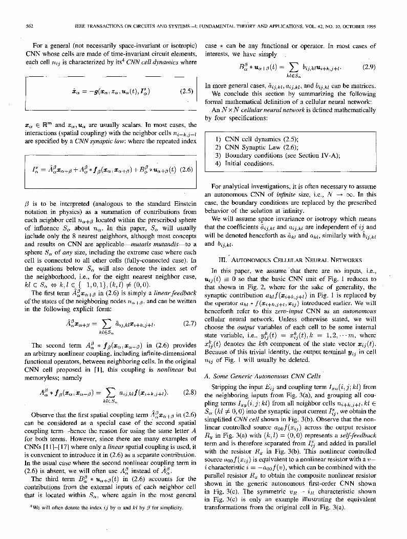
Another CNN cell that has been widely used for pattern formation and active wave propagation [ 1 l]-[ 171 is the generic autonomous third-order CNN cell shown in Fig. 4(a) and (b). Observe that this circuit reduces to Chua’s circuit [18] upon short circuiting the resistor Ro and setting the synaptic currents I%? and I,$ to zero. The state equations of this generic cell are given by

iij = k[-yij - Rozij]. (3.1)

For analytical 0~ simulation purposes, it is often more convenient to use the following dimensionless version of (3.1) [18]:

(3.2)

Again, this CNN cell dynamics contains only one nonlinearity h(.), which may be any (not necessarily symmetric or Piecewise-linear) scalar nonlinear function h: Iw + R.

In general, we can define a CNN cell of any order n > 3, with multiple synaptic coupling, as depicted in Fig. 4(c).

B. Linear Synaptic Laws via Resistor Couplings

In this paper, we will focus on an important subclass of autonomous CNN defined by the following linear synaptic law:

I& = c ~klxi+k,j+l (3.3) k,lG{-l,O,l}

(kd)#(O.O)

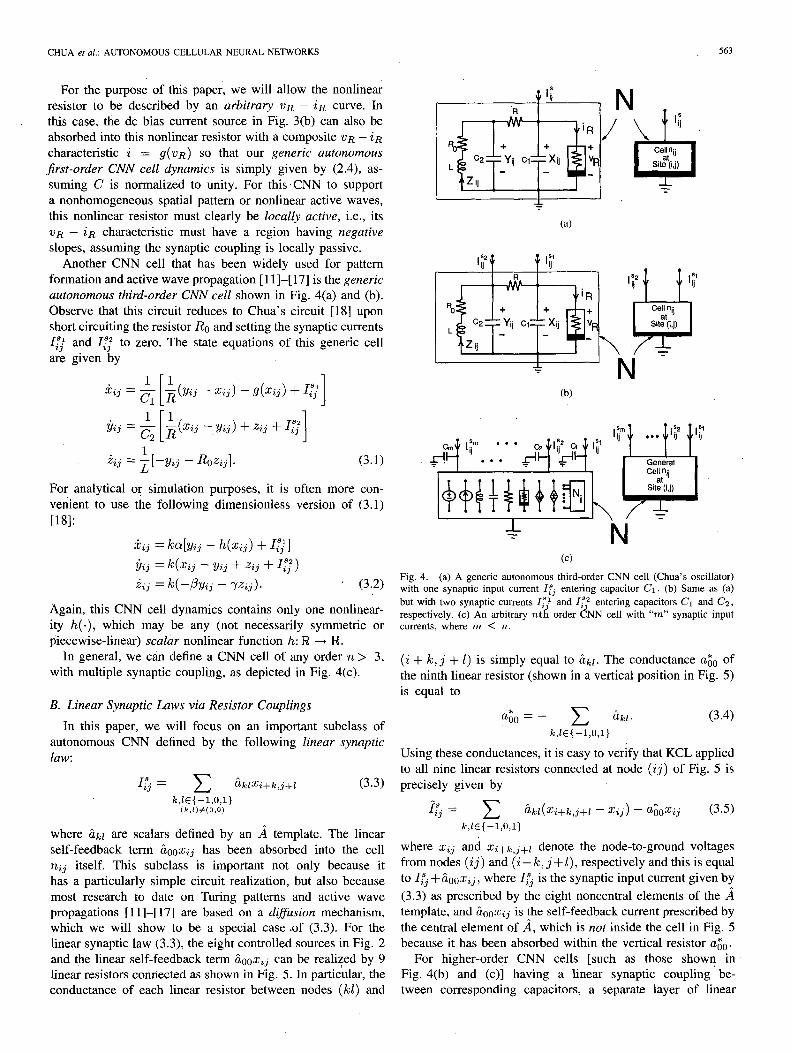
where i&l are scalars defined by an a template. The linear self-feedback term &,x~j has been absorbed into the cell nij itself. This subclass is important not only because it has a particularly simple circuit realization, but also because most research to date on Turing patterns and active wave propagations [l l]-[17] are based on a difSusion mechanism, which we will show to be a special case .of (3.3). For the linear synaptic law (3.3), the eight controlled sources in Fig. 2 and the linear self-feedback term iLooZij can be reali:ed by 9 linear resistors connected as shown in Fig. 5. In particular, the conductance of each linear resistor between nodes (kl) and

1.; ‘R iR m / Ro + + + CP

L Yij Cl Xij ”

zij- - -

(4

r- R iFl % + + + m CP L

Yij Cl Xij “F Z ij

L -

(b)

N / \ y

id T ii

Site (i,j)

1; ... 1% I;

General

Yii Site (i.j)

\ tri T

Cc) Fig. 4. (a) A generic autonomous third-order CNN cell (Chua’s oscillator) with one synaptic input current It3 entering capacitor C1. (b) Same as (a) but with two synaptic currents If,’ and Iz”, entering capacitors C’1 and Cz, respectively. (c) An arbitrary nth order CNN cell with “m ” synaptic input currents, where m 5 R.

(i + k, j + 1) is simply equal to &l. The conductance aGo of the ninth linear resistor (shown in a vertical position in Fig. 5) is equal to

ago = - c ;kl. k,&{-l,O,l}

(3.4)

Using these conductances, it is easy to verify that KCL applied to all nine linear resistors connected at node (ij) of Fig. 5 is precisely given by

f$ Ix c &kl(xi+k,j+l - xij) - &+ij (3.5) kc,&{-l,O,l}

where xij and Xc;+!++1 denote the node-to-ground voltages from nodes (ij) and (i + k, j + Z), respectively and this is equal to Itj + iLooxij, where I$ is the synaptic input current given by (3.3) as prescribed by the eight noncentral elements of the a template, and &ooZij is the self-feedback current prescribed by the central element of a, which is not inside the cell in Fig. 5 because it has been absorbed within the vertical resistor agO.

For higher-order CNN cells [such as those show? in Fig. 4(b) and (c)] having a linear synaptic coupling between corresponding capacitors, a separate layer of linear

564 IEEE TRANSACTIONS ON CIRCUITS AND SYSTEMS--I: FUNDAMENTAL THEORY AND APPLICATIONS, VOL. 42, NO. 10, OCTOBER 1995

,* ‘8’ 00

t (iJ+U . 0.1

@

%,l

i -1 ,o (i-1 ,I+1 )

(l-1 J)

“-8 1 ii

i template -

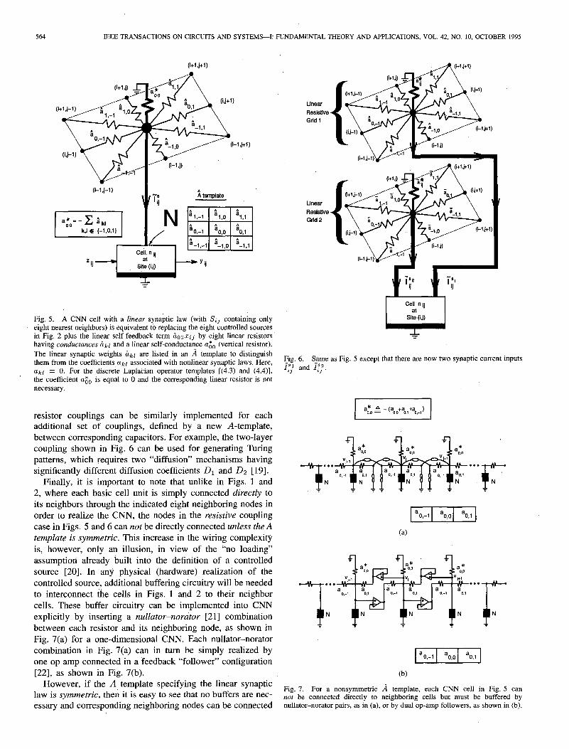
Fig. 5. A CNN cell with a linear synaptic law (with S;j containing only eight nearest neighbors) is equivalent to replacing the eight controlled sources in Fig. 2 plus the linear self-feedback term &nz;j by eight linear resistors having conductunces ckl and a linear self-conductance agO (vertical resistor). The linear synaptic weights Gkl are listed in an A template to distinguish them from the coefficients akr associated with nonlinear synaptic laws. Here, akl = 0. For the discrete Laplacian operator templates [(4.3) and (4.4)], the coefficient cc0 is equal to 0 and the corresponding linear resistor is not necessary.

resistor couplings can be similarly implemented for each additional set of couplings, defined by a new A-template, between corresponding capacitors. For example, the two-layer coupling shown in Fig. 6 can be used for generating Turing patterns, which requires two “diffusion” mechanisms having significantly different diffusion coefficients Di and Ds [19].

Finally, it is important to note that unlike in Figs. 1 and 2, where each basic cell unit is simply connected directly to its neighbors through the indicated eight neighboring nodes in order to realize the CNN, the nodes in the resistive coupling case in Figs. 5 and 6 can not ,be directly connected unless the A template is symmetric. This increase in the wiring complexity is, however, only an illusion, in view of the “no loading” assumption already built into the definition of a controlled source [20]. In any physical (hardware) realization of the controlled source, additional buffering circuitry will be needed to interconnect me cells in Figs. 1 and 2 to their neighbor cells. These buffer circuitry can be implemented into CNN explicitly by inserting a nullator-norbtor [21] combination between each resistor and its neighboring node, as shown in Fig. 7(a) for a one-dimensional CNN. Each nullator-norator combination in Fig. 7(a) can in turn be simply realized by one op amp connected in a feedback “follower” configuration [22], as shown in Fig. 7(b).

However, if the A template specifying the linear synaptic law is symmetric, then it is easy to see that no buffers are nec- essarv and corresuondina neiehborine nodes can be connected

Linear Resistive - Grid 1

hear Resistive - Grid 2

I “=Yt ” ii Site 0.1) I T

Fig. 6. Same as Fig. 5 except that there are now two synaptic current inputs i”: and j!?,

23 13

I a* !Y -(a +a +a 0.0 - 0.0 0.1 O.-l ) I

(b) Fig. 7. For a nonsymmetric a template, each CNN cell in Fig. 5 can not be connected directly to neighboring cells but must be buffered by nullator-norator pairs, as in (a), or by dual op-amp followers, as shown in (b).


directly, as will be the case in realizing the reaction-d@usion CNNs in the next section. This class of autonomous CNN consists of mth order cells (m 2 1) coupled to each other by one or more layers of linear resistors. They are described mathematically by the state equations

i: = f(z) + AZ (3.6)

where z E Wmn2 for an n x n CNN, and A is-a band matrix qf dimension mn2 x mn2 (assuming the cells are numbered consecutively from left to right and from top to bottom). For example, a 100 x 100 reaction-diffusion CNN made of the generic third-order cells shown in Fig. 4(a) would consist of 3 x lo4 nonlinear ordinary differential equations.

IV. REACTION-DIFFUSION CELLULAR NEURAL NETWORKS In this section, we present several standard autonomous

CNN architectures that can be designed to generate patterns and waves, including trigger waves (autowaves), target (concentric) waves, spiral waves, and scroll waves (for three- dimensional CNNs) [l l]-[17]. These CNNs will be called reaction-diffusion CNNs because they are described mathematically by a discretized version of the following well-known system of nonlinear partial differential equations-generally referred to in the literature as reaction-diffusion equations [ 1915:

where u E W”, f E W”, D is an m x m diagonal matrix whose diagonal elements Di are called the diffusion coefficients, and

A d2Ui d2Ui v2ui = - -

ax2 + dy2 ' i = 1,2,...,m (4.2)

is the Laplacian operator in R2. There are several ways to approximate the Laplacian op-

erator V2ui in discrete space by a CNN synaptic law with an appropriate A-template [23]. In this paper, we will choose the following templates for one- and two-dimensional reaction-diffusion CNNs:

I) One-dimensional discretized Laplacian template Al

AI: /11-2/1/ (4.3)

2) Two-dimensional discretized Laplacian template A2

(4.4)

Note that this is a special case of the synaptic law (3.3). Since the coefficients of the template Al and A2 sum to zero, in the resistor coupling realization of Fig. 5, the resistor uzo can be deleted.

5 We will often follow the usual notation in the literature [ 191 by choosing u;j for state variables and (2, y) for spatial variables in R2.

q...~..~,

(4

D

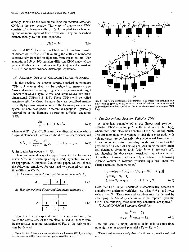
(b) Fig. 8. (a) A one-dimensional autonomous CNN whose end terminals can either tend to &x as in the case of a CNN of infinite size or terminated by prescribed boundary conditions. (b) A one-dimensional autonomous CNN Ring.

A. One-Dimensional Reaction-Di#usion CNN

A canonical example of a one-dimensional reaction- diffusion CNN containing N cells is shown in Fig. 8(a), where each solid black box denotes a CNN cell of any order. The left-most node with voltage u. and right-most node with voltage ZIN+~ are deliberately left unconnected here in order to accommodate various boundary conditions, as well as the possibility of a CNN of injinite size. Assuming the third-order cell dynamics given by (3.2) (with k = 1) for each celi, and choosing the above one-dimensional Laplacian template Al with a diffusion coefficient D1 we obtain the following discrete version of reactidn-diffusion equations (Here, we chang6 notation from wj to x~j):

izi = a[yi - h(xi) + D(x+ - 2xj - q+l)] ?jj = xj - yj + zj ij = -py.j - yzj j = 1,2;..,N. (4.5)

Note that (4.5) is yet undefined mathematically because it contains two undefined variables-x0 (when j = 1) and xiv+1 (when j = N). These two end variables must be defined by specifying the boundary conditions to be imposed upon the CNN. The following three boundary conditions are typical.6

1) Fixed (Dirichlet) Boundary Condition:

x0 !I 210 = El

xN+l 2 UN+1 = E2. (4.6)

Here, the CNN is simply clamped at its ends to some fixed potential, say at ground potential (El = E2 = 0).

6Pattems and waves are usually observed with boundary conditions (2) and (3).

566 IEEE TRANSACTIONS ON CIRCUITS AND SYSTEMS-I: FUNDAMENTAL THEORY AND APPLICATIONS, VOL. 42, NO. 10, OCTOBER I995

2) Zero-Flux (Neumann) Boundary Condition:

x0 e 210 = ?I1 A

xN+l = UN+1 = UN. (4.7)

Equation (4.7) is the discrete version of the zero-outward derivative condition du/dx = 0 imposed at each end of a one- dimensional continuum medium. When using a standard circuit simulator, (4.7) can be implemented by connecting a unity- gain voltage-controlled voltage source from each end node to ground and controlled by the node voltage of its neighbor.

3) Periodic (Ring) Boundary Condition: A

x,, = ‘&, = UN A

xN+l = t’N+l =2)1. (4.8)

This boundary condition is equivalent to connecting the two ends of the CNN in Fig. 8(a) together (after deleting one of the two end resistors) to obtain the CNN ring shown in Fig. 8(b).

Every known trigger wave7 phenomena from continuum media (e.g., chemical reaction, combustion, epidemic wave, etc.) that have been reported to date in the literature have also been successfully simulated by a one-dimensional CNN, often with only a relatively small N 2 50 [l l]-[17]. This observation may not appear surprising since as N + co, (4.5) approaches the nonlinear partial differential equation (4.1). What is surprising is that this intuitively reasonable observation is true only in one direction: there exists some phenomena, e.g., the propagation failure phenomenon, in a one-dimensional CNN, which can be proved [24] to be im- possible to occur in its associated reaction-diffusion partial differential equation [l l] as N --) 0~). Roughly speaking, the “propagation failure” phenomenon is said to occur when a voltage pulse traveling along a CNN (with diffusion coefficient 0) at velocity ?~g > 0 suddenly stops propagating (i.e., 21~1 = 0) when D is reduced below some small but positive value. This phenomenon is similar to the nerve propagation failure phenomenon widely reported from patients suffering from multiple sclerosis: beyond a certain stage of this dreaded disease, pinching the patient’s finger tip will no longer elicit a painful sensation. Neurologists have spent many years trying to simulate and explain this phenomenon using (4.1) without success until proven only recently in [24] to be impossi- ble. The fact that a one-dimensional CNN has no problem producing this phenomenon shows in some sense that the class of reaction-diffusion CNN is more general than its continuum version modeled by a nonlinear partial differential equation. This observation is counter-intuitive and could have far reaching significance, even for no other applications than a mere understanding of some possible mechanisms that can cause nerve transmission failure.

B. Two-Dimensional Reaction-Diffksiom CNN

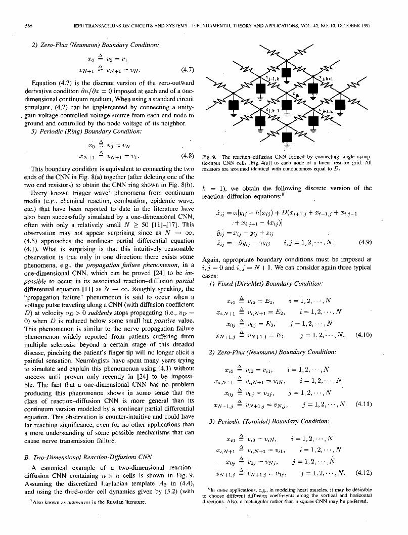
A canonical example of a two-dimensional reaction- diffusion CNN containing n x n cells is shown in Fig. 9. Assuming the discretized Laplacian template A2 in (4.4), and using the third-order cell dynamics given by (3.2) (with

7Also known as autowaves in the Russian literature.

Fig. 9. The reactiondiffusion CNN formed by connecting single synaptic-input CNN cells [Fig. 4(a)] to each node of a linear resistor grid. All resistors are assumed identical with conductances equal to D.

k = l), we obtain the following discrete version of the reaction-diffusion equations:8

iii = 4Yij - h(Xij) + D(Xi+1,j + x;-1,j + x;,j-1 ’ + xi,j+1 - 4Gj)]

?kj = xij - yij + z;j .iij = -py;.j - 7zi.j i,j = 1,2,...,N. (4.9)

Again, appropriate boundary conditions must be imposed at i, j = 0 and i, j = N + 1. We can consider again three typical cases:

1) Fixed (Dirichlet) Boundary Condition:

xi(J a vi0 = El, i= 1,2,..,,N

xi,N+l b ‘u&N+1 = ~72, i = 1,2,...,N A

xoj = ‘uoj = E3, j = 1,2;..,N A

xN+l,j = vN+l,j = E4r j = 1,2&N. (4.10)

2) Zero-Flux (Neumann) Boundary Condition:

A Xi0 = Vi0 = Vii, i = 1,2,...,N

xi,N+l ’ vi,N+l = ViN, i = 1,2,. . , N A

xoj = “Oj = wpj, j = 1,2,...,N A

xN+l,i = vN+l,j = vN,j, j = 1,2,...,N. (4.11)

3) Periodic (Toroidal) Boundary Condition:

Xi0 A ViO=Vihfy i = 1,2,...,N A

xi,N+l = ‘%,N+l = ‘uil, i = 1,2,...,N A

“oj = V,,j =VNj, j = 1,2,...,N

xN+l,i ’ “‘N+l,j = vlj, j = 1,2,...,N. (4.12)

81n some applications, e.g., in modeling heart muscles, it may be desirable to choose different diffusion coefficients along the vertical and horizontal directions. Also, a rectangular rather than a square CNN may be preferred.

CHUA et al.: AUTONOMOUS CELLULAR NEURAL NETWORKS

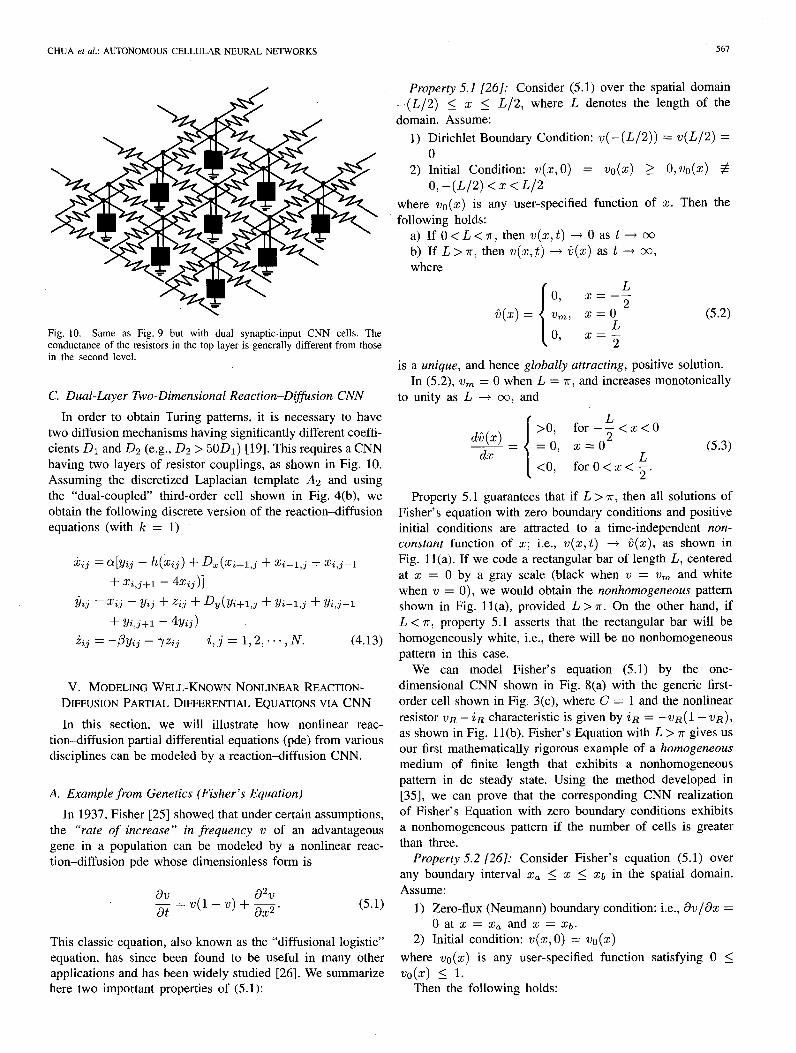
Fig. 10. Same as Fig. 9 but with dual synaptic-input CNN cells. The conductance of the resistors in the top layer is generally different from those in the second level.

C. Dual-Layer Two-Dimensional Reaction-Diffusion CNN

In order to obtain Turing patterns, it is necessary to have two diffusion mechanisms having significantly different coefficients D1 and D2 (e.g., 02 > 5001) [19]. This requires a CNN having two layers of resistor couplings, as shown in Fig. 10. Assuming the discretized Laplacian template A2 and using the “dual-coupled” third-order cell shown in Fig. 4(b), we obtain the following discrete version of the reaction-diffusion equations (with k = 1)

‘ii = a[Yij - h(kij) + D,(xi+l,j + xi-l,j + xi,j-l + Xi,j+l - 4Xij)]

yij = Xij - ~ij + ‘ii + D,(YY;+I,~ + yi-l,j + yi,j-l + Yi,j+l - 4Yij)

iij = -@yij - yzij i,j = 1,2;. . ,N. (4.13)

V. MODELING WELL-KNOWN NONLINEAR REACTION- DIFFUSION PARTIAL DIFFERENTIAL EQUATIONS VIA CNN

In this section, we will illustrate how nonlinear reaction-diffusion partial differential equations (pde) from various disciplines can be modeled by a reaction-diffusion CNN.

A. Example from Genetics (Fisher’s Equation)

In 1937, Fisher [25] showed that under certain assumptions, the “rate of increase” in frequency v of an advantageous gene in a population can be modeled by a nonlinear reaction-diffusion pde whose dimensionless form is

dv - = v(1 - v) + g. at

This classic equation, also known as the “diffusional logistic” equation, has since been found to be useful in many other applications and has been widely studied [26]. We summarize here two imuortant nronerties of (5.1):

Property 5.1 [26]: Consider (5.1) over the spatial domain -(L/2) 5 x 5 L/2, where L denotes the length of the domain. Assume:

1) Dirichlet Boundary Condition: v(-(L/2)) = v(L/2) = 0

2) Initial Condition: v(x,O) = Q(X) > 0, Q(X) $ 0, -(L/2) <x < L/2

where vo(x) is any user-specified function of 2. Then the following holds:

a) If O<L<r, then v(x,t) + 0 as t + cc b) If L > X, then v(x,j) -+ G(x) as t --+ CS, where

L 0, xx--

G(x) = 2

vm, x=0 (5.2) r 0, x2

2

is a unique, and hence globally attracting, positive solution. In (5.2), v, = 0 when L = 7r, and increases monotonically

to unity as L --+ co, and

dG(x) >o, for -‘<x<O - =

dx =o, x = o2 (5.3)

a forO<x<g.

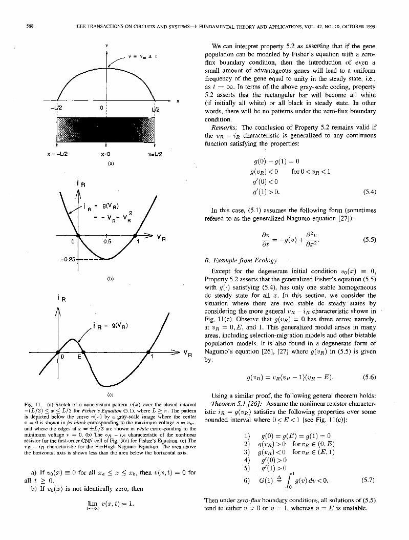
Property 5.1 guarantees that if L > n, then all solutions of Fisher’s equation with zero boundary conditions and positive initial conditions are attracted to a time-independent nonconstant function of x; i.e., v(x, t) + G(x), as shown in Fig. 11(a). If we code a rectangular bar of length L, centered at x = 0 by a gray scale (black when v = v, and white when v = 0), we would obtain the nonhomogeneous pattern shown in Fig. 11(a), provided L > n-. On the other hand, if L < r, property 5.1 asserts that the rectangular bar will be homogeneously white, i.e., there will be no nonhomogeneous pattern in this case.

We can model Fisher’s equation (5.1) by the one- dimensional CNN shown in Fig. 8(a) with the generic first- order cell shown in Fig. 3(c), where C = 1 and the nonlinear resistor ‘UR - iR characteristic is given by iR = -vR( 1 - VR), as shown in Fig. 1 l(b). Fisher’s Equation with L > x gives us our first mathematically rigorous example of a homogeneous medium of finite length that exhibits a nonhomogeneous pattern in dc steady state. Using the method developed in [35], we can prove that the corresponding CNN realization of Fisher’s Equation with zero boundary conditions exhibits a nonhomogeneous pattern if the number of cells is greater than three.

Property 5.2 [26]: Consider Fisher’s equation (5.1) over any boundary interval xa ‘5 x 5 x6 in the spatial domain. Assume:

1) Zero-flux (Neumann) boundary condition: i.e., dv/dx = 0 at x = xa and x = Xb.

2) Initial condition: v(x,O) = vo(x) where Q(X) is any user-specified function satisfying 0 5 vo(x) 5 1.

Then the followine holds:

568 IEEE TRANSACTIONS ON CIRCUITS AND SYSTEMS--I: FUNDAMENTAL THEORY AND APPLICATIONS, VOL. 42, NO. 10, OCTOBER 1995

x=0 (a)

(b)

> “R

(cl Fig. 11. (a) Sketch of a nonconstant pattern V(Z) over the closed interval -(L/2) 5 z 5 L/2 for Fisher’s Equation (5.1), where L 2 a. The pattern is depicted below the curve V(Z) by a gray-scale image where the center z = 0 is shown in jet black corresponding to the maximum voltage u = om , and where the edges at z = &L/2 are shown in white corresponding to the minimum voltage 2) = 0. (b) The VR - in characteristic of the nonlinear resistor for the first-order CNN cell of Fig. 3(c) for Fisher’s Equation. (c) The VR - in characteristic for the FitzHugh-Nagumo Equation. The area above the horizontal axis is shown less than the area below the horizontal axis,

a) If wu(5) = 0 for all z a 5 x 5 xb, then w(~,t) = 0 for all t 2 0.

b) If va(z) is not identically zero, then

,lim w(s,t) = 1. t-+cc

We can interpret property 5.2 as asserting that if the gene population can be modeled by Fisher’s equation with a zero- flux boundary condition, then the introduction of even a small amount of advantageous genes will lead to a uniform frequency of the gene equal to unity in the steady state, i.e., as t -+ 00. In terms of the above gray-scale coding, property 5.2 asserts that the rectangular bar will become all white (if initially all white) or all black in steady state. In other words, there will be no patterns under the zero-flux boundary condition.

Remarks: The conclusion of Property 5.2 remains valid if the ‘UR - in characteristic is generalized to any continuous function satisfying the properties:

g(O) =9(l) = 0 d’uR) < 0 forO<uR<l

g’(O) < 0 g’(1) > 0. -(5.4)

In this case, (5.1) assumes the following form (sometimes refered to as the generalized Nagumo equation [27]):

dv - = -g(w) + g. at (5.5)

B. Example from Ecology

Except for the degenerate initial condition vu(~) c 0, Property 5.2 asserts that the generalized Fisher’s equation (5.5) with g(.) satisfying (5.4), has only one stable homogeneous dc steady state for all x. In this section, we consider the situation where there are two stable dc steady states by considering the more general ?JR - iR characteristic shown in Fig. 11(c). Observe that g(wR) = 0 has three zeros; namely, at 21~ = 0, E, and 1. This generalized model arises in many areas, including selection-migration models and other bistable population models. It is also found in a degenerate form of Nagumo’s equation [26], 1271 where g(vR) in (5.5) is given by:

g(vR) = wR(w~ - l)(wR - E). (5.6)

Using a similar proof, the following general theorem holds: Theorem 5. I [26]: Assume the nonlinear resistor character-

istic iR = g(VR) satisfies the following properties Over some bounded interval where 0 <: E < 1 [see Fig. 1 I(c)]:

1) do) = g(E) = g(1) = 0 2) g(wR) > 0 for wR E (0, E) 3) g(uR) < 0 forvR E (E, 1) 4) g’(O) > 0 5) g’(l) > 0

1

6) G(1) e s 0 g(w) dw < O.

(5.7)

Then under zero-flux boundary conditions, all solutions of (5.5) tend to either w = 0 or u = 1, whereas v = E is unstable.


Theorem 5.1 asserts that the limiting form of the one- dimensional reaction-diffusion CNN in Fig. 8(a) having first- order cells (see Fig. 3(c)) satisfying (5.7) -with C = 1 and zero-flux boundary conditions has a b&able steady state.

Many electronic devices and circuits can be synthesized, with appropriate dc bias, to obtain a WR - in characteristic satisfying (5.7), such as the curve shown in Fig. 11(c). Note that condition 6 of (5.7) means that the area bounded by the VR - iR characteristic above the UR-axis must be smaller than that below the VR-axis. This condition is easily realized by connecting a dc current source in parallel with the nonlinear resistor as in the first-order CNN cell in Fig. 3(c). Moreover, by connecting a dc voltage source in series with the resulting nonlinear resistor, the VR-~R curve of the composite nonlinear resistor (i.e., including the parallel current source and series battery) resembles the nonlinear curve of Fig. 1 l(c) (except for its piecewise-linear character) and satisfies (5.7). Since the introduction of the series battery clearly does not affect the qualitative dynamics of the resulting state equations, it is expected that the autonomous reaction diffusion CNN made of such first-order cells will behave like Theorem 5.1 when the number of cells is sufficiently large; namely, we have two (b&able) dc steady states. This conclusion is similar to the complete stability theorem proved in [l]. By choosing appropriate initial conditions, a traveling “trigger” or “auto” wave can be initiated that switches from one stable state to the other [ll], [12]. Such phenomena have been exploited for global optimization and image processing applications.

C. Example from Mathematical Biology (FitzHugh-Nagumo Equation)

The most widely-used mathematical model of excitation and propagation of impulse (action potential) in nerve membranes is the FitzHugh-Nagumo Equation whose dimensionless form is given by [19], [28]

?&-(~~*)~y+!?!g dY -=&(X--Y) at

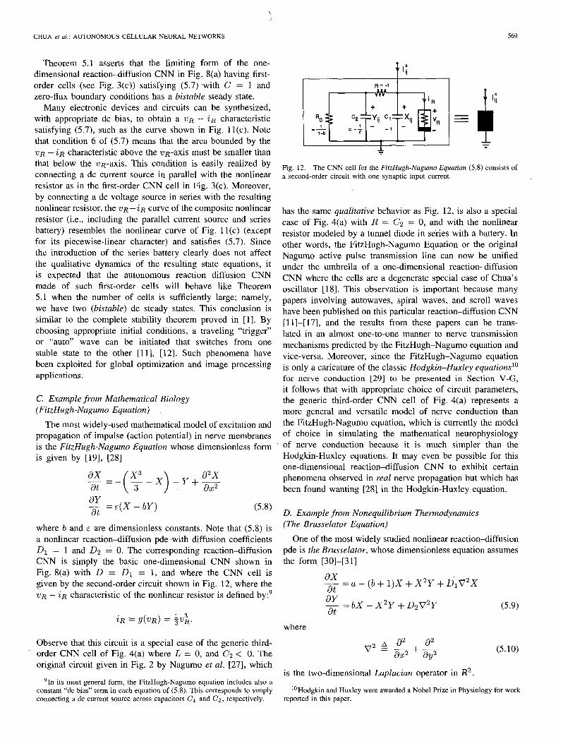
where b and E are dimensionless constants. Note that (5.8) is a nonlinear reaction-diffusion pde with diffusion coefficients D1 = 1 and 02 = 0. The corresponding reaction-diffusion CNN is simply the basic one-dimensional CNN shown in Fig. 8(a) with D = D1 = 1, and where the CNN cell is given by the second-order circuit shown in Fig. 12, where the VR - iR characteristic of the nonlinear resistor is defined by:9

iR = g(?&) = +;.

Observe that this circuit is a special case of the generic third- order CNN cell of Fig. 4(a) where L = 0, and Cz < 0. The original circuit given in Fig. 2 by Nagumo et al. [27], which

91n its inost general form, the FitzHugh-Nagumo equation includes also a constant “dc bias” term in each equation of (5.8). This corresponds to simply connecting a dc current source across capacitors Cl and Cz, respectively.

Fig. 12. The CNN cell for the FitzHugh-Nagumo Equation (5.8) consists of a second-order circuit with one synaptic input current.

has the same qualitative behavior as Fig. 12, is also a special case of Fig. 4(a) with R = C, = 0, and with the nonlinear resistor modeled by a tunnel diode in series with a battery. In other words, the FitzHugh-Nagumo Equation or the original Nagumo active pulse transmission line can now be unified under the umbrella of a one-dimensional reaction-diffusion CNN where the cells are a degenerate special case of Chua’s oscillator [ 181. This observation is important because many papers involving autowaves, spiral waves, and scroll waves have been published on this particular reaction-diffusion CNN [l l]-[17], and the results from these papers can be trans- lated in an almost one-to-one manner to nerve transmission mechanisms predicted by the FitzHugh-Nagumo equation and vice-versa. Moreover, since the FitzHugh-Nagumo equation is only a caricature of the classic Hodgkin-Huxley equations’0 for nerve conduction [29] to be presented in Section V-G, it follows that with appropriate choice of circuit parameters, the generic third-order CNN cell of Fig. 4(a) represents a more general and versatile model of nerve conduction than the FitzHugh-Nagumo equation, which is currently the model of choice in simulating the mathematical neurophysiology of nerve conduction because it is much simpler than the Hodgkin-Huxley equations. It may even be possible for this one-dimensional reaction-diffusion CNN to exhibit certain phenomena observed in real nerve propagation but which has been found wanting [28] in the Hodgkin-Huxley equation.

D. Example from Nonequilibrium Thermodynamics (The Brusselator Equation)

One of the most widely studied nonlinear reaction-diffusion pde is the Brusselator, whose dimensionless equation assumes the form, [30]-[31]

dX -=a-((b+1)X+X2Y+D;V2X

ifi - = bX - X2Y + D2V2Y at

where

(5.10)

is the two-dimensional Laplacian operator in R2.

loHodgkin and Huxley were awarded a Nobel Prize in Physiology for work reported in this paper.

570 IEEE TRANSACTIONS ON CIRCUITS AND SYSTEMS-I: FUNDAMENTAL THEORY AND APPLICATIONS, VOL. 42, NO, 10, OCTOBER 1995

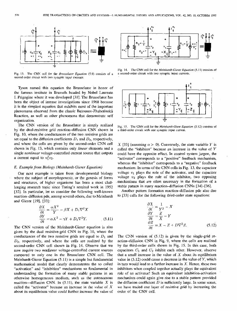
Fig. 13. The CNN cell for the Brusselaror Equation (5.9) consists of a second-order circuit with two synaptic input currents.

Tyson named this equation the Brusselator in honor of the famous institute in Brussels headed by Nobel Laureate I. Prigogine where it was developed [31]. The Brusselator has been the object of intense investigations since 1968 because it is the simplest equation that exhibits most of the important phenomena observed from the classic Belousov-Zhabotinskii Reaction, as well as other phenomena that demonstrate self organization.

The CNN version of the Brusselator is simply realized by the dual-resistive grid reaction-diffusion CNN shown in Fig. 10, where the conductances of the two resistive grids are set equal to the diffusion coefficients Dr and D2, respectively, and where the cells are given by the second-order CNN cell shown in Fig. 13, which contains only linear elements and a single nonlinear voltage-controlled current source that outputs a current equal to $212.

E. Example from Biology (Meinhardt-Gierer Equation)

Our next example is taken from developmental biology where the subject of morphogenesis, or the genesis of forms and structures, of higher organisms has been a most challenging research topic since Turing’s seminal work in 1952 [32]. In particular, let us consider the following well-known reactiondiffusion pde, among several others, due to Meinhardt and Gierer [19], [33]:

8X ax2 -=-

:h Y

- ,8X + D1V2X

_ zz ax2 - yY + D2V2Y. at

The CNN version of the Meinhardt-Gierer equation is also given by the dual resistive-grid CNN in Fig. 10, where the conductances of the two resistive grids are equal to D1 and D2, respectively, and where the cells are realized by the second-order CNN cell shown in Fig. 14. Observe that we now require two nonlinear voltage-controlled current sources compared to only one in the Brusselator CNN cell. The Meinhardt-Gierer Equation (5.11) is a simple but fundamental mathematical model that clearly demonstrates the so called “activation” and “inhibition” mechanisms so fundamental in understanding the formation of many stable patterns in an otherwise homogeneous medium, such as the autonomous reaction-diffusion CNN. In (5.1 l), the state variable X is called the “activator” because an increase in the value of X about its equilibrium value could further increase the value of

Fig. 14. The CNN cell for the Meinhardt-Gierer Eq’ktion (5.11) consists of a second-order circuit with two synaptic input currents.

Fig. 15. The CNN cell for the Meinhardr-Giere Equation (5.12) consists of a third-order circuit with one synaptic input current.

X [33] (assuming Q: > 0). Conversely, the state variable Y is called the “inhibitor” because an increase in the value of Y could have the opposite effect. In control system jargon, the “activator” corresponds to a “positive” feedback mechanism, whereas the “inhibitor” corresponds to a “negative” feedback mechanism. In terms of the CNN cells in Fig. 13, the capacitor voltage wr plays the role of the activator, and the capacitor voltage 212 plays the role of the inhibitor, two opposing mechanisms that are often necessary in the formation of a stable pattern in many reaction-diffusion CNNs [34]-[36].

Another pattern formation reaction-diffusion pde also due to [33] calls for the following third-order state equations:

ax 1 ----x

z-

ii

TY -=-.-

- =X:Z+DV’Z. at

(5.12)

The CNN version of (5.12) is given by the single-grid reaction-diffusion CNN in Fig. 9, where the cells are realized by the third-order cells shown in Fig. 15. In this case, both capacitors Cr and Cz inhibit each other. However, observe that a small increase in the value of X about its equilibrium value in (5.12) could cause a decrease in the value of Y, which in turn would lead to a further increase in X. Hence, these two inhibitors when coupled together actually plays the equivalent role of an activator! Such an equivalent inhibition-activation mechanism could again give rise to a stable pattern provided the diffusion coefficient D is sufficiently large. In some sense, we have traded one layer of resistive grid by increasing the order of the CNN cell.

CHUA et al.: AUTQNOMOUS CELLULAR NEURAL NETWORKS 571

F. Example from Chemistry (Oregonator Equation)

A more complicated but realistic model of the spiral wave phenomenon observed in the well-known Belousov- Zhabotinskii Reaction [30] in chemistry has been described by Field and Noyes at the University of Oregon in 1974 [37] and called the Oregonator to relate it to the simpler but less realistic Brusselator.

The dimensionless form of the Qregonator is given by: .’

E~=X+Y-Q,X~-XY+D~V~X

8Y -=-Y+pZ-XY+D2V2Y at

6g=X-Z+D,V”Z. (5.13)

Assuming the most general case where there are three diffusion coefficients D1, D2, and Ds, we can realize a corresponding Oregonator CNN consisting of three resistive grids whose conductances are set equal to Dl,D2, and 03, respectively.

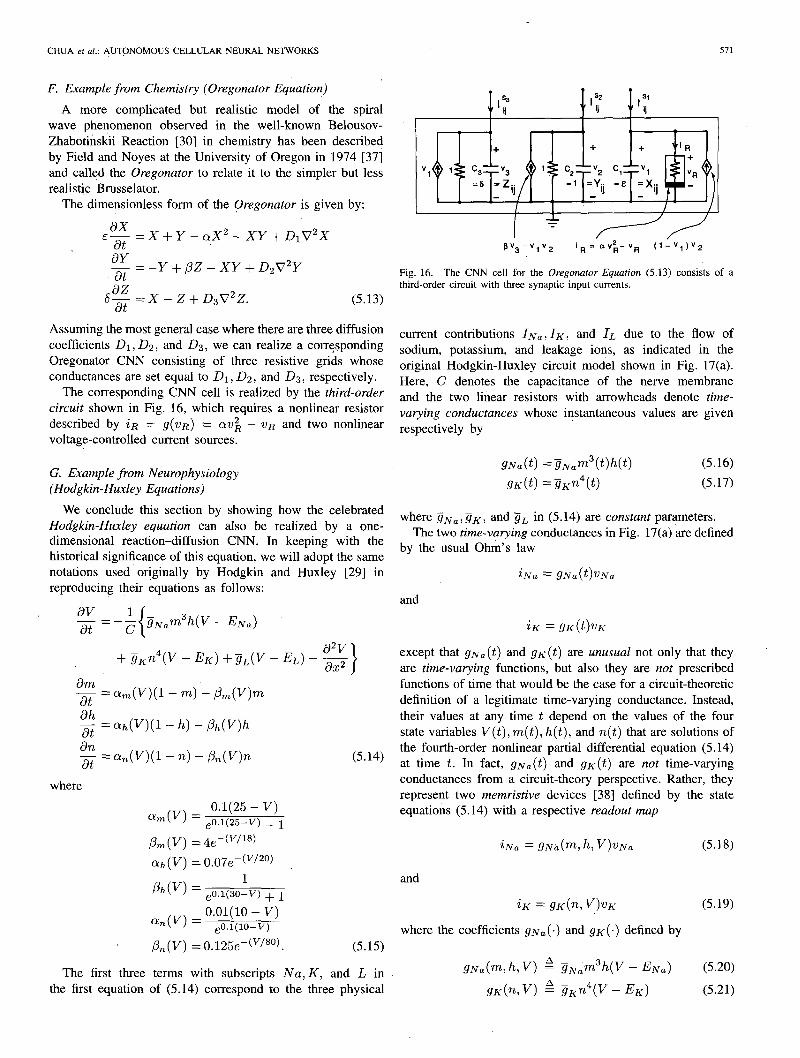
The corresponding CNN cell is realized by the third-order circuit shown in Fig. 16, which requires a nonlinear resistor described by in = g(wR) = WV& - OR and two nonlinear voltage-controlled current sources.

G. Example from Neurophysiology (Hodgkin-Huxley Equations)

We conclude this section by showing how the celebrated Hodgkin-Huxley equation can also be realized by a one- dimensional reaction-diffusion CNN. In keeping with the historical significance of this equation, we will adopt the same notations used originally by Hodgkin and Huxley [29] in reproducing their equations as follows:

dV 1 at=-c gNam3h(V -ENS)

+ gKn4(V - EK) + sL(V - EL) - g

$ =@b~(V)(l- m) - &(V)m

2 = m(V)(l - h) - /‘&(V)h

g = Lyn(V)(l - n) - P,(V), (5.14)

where

&n(V) = 0.1(25 - V)

e0.1(25-V) _ 1

pm(v) = 4e-(V/18)

cYh(V) = 0.07e-(V’20)

Ph(V) = l eo.1(30-v) + 1

Qn(V) = O.Ol(lO - V)

eo.l(lo-v)

,&(V) = 0.125e-(V/80). (5.15)

The first three terms with subscripts Na, K, and L in the first equation of (5.14) correspond to the three physical

Fig. 16. The CNN cell for the Oregonator Equation (5.13) consists of a third-order circuit with three synaptic input currents.

current contributions IN,, IK, and IL due to the flow of sodium, potassium, and leakage ions, as indicated in the original Hodgkin-Huxley circuit model shown in Fig. 17(a). Here, C denotes the capacitance of the nerve membrane and the two linear resistors with arrowheads denote time- varying conductances whose instantaneous values are given respectively by

gNa(t) = %vam3(t)h(t) gK(t) =SKn4(t)

(5.16) (5.17)

where gNa, ijK, and ?jL in (5.14) are constant parameters. The two time-varying conductances in Fig. 17(a) are defined

by the usual Ohm’s law

iNa = gNa(+‘Na

and

iK = gK(t)VK

except that gNa(t) and gK(i!) are unusual not only that they are time-varying functions, but also they are not prescribed functions of time that would be the case for a circuit-theoretic definition of a legitimate time-varying conductance. Instead, their values at any time t depend on the values of the four state variables V(t), m(t), h(t), and n(t) that are solutions of the fourth-order nonlinear partial differential equation (5.14) at time t. In fact, gNa(t) and gK(t) are not time-varying conductances from a circuit-theory perspective. Rather, they represent two memristive devices [38] defined by the state equations (5.14) with a respective readout map

iNa = gNh.(m, h, v)wNa

and

iK = gK(% v)vK

where the coefficients gNa(‘) and gK (.) defined by

gNa(m, h, V) a gNam3h(V - ENS)

gK(n, v) 2 jjKn4(V - EK)

(5.18)

(5.19)

(5.20)

(5.21)


1 (a)

5

E

(b)

+

El-

a, (v)(l-n)-p,w n 1

1 (cl

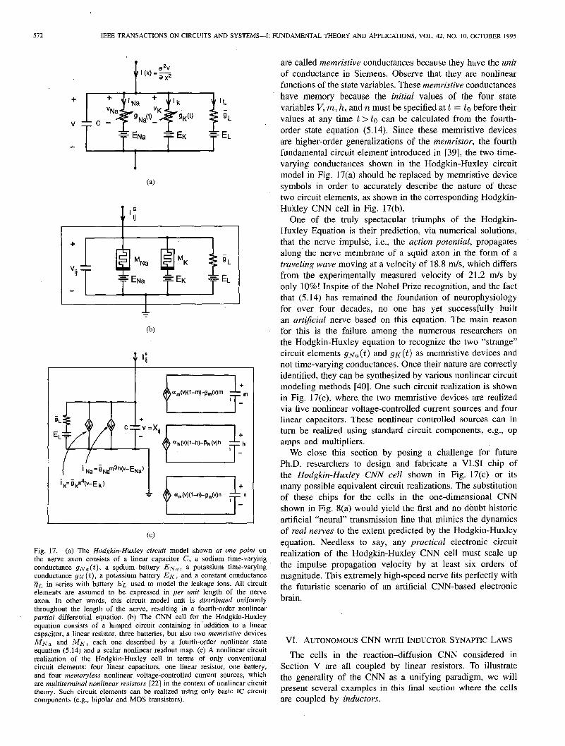
Fig. 17. (a) The Hodgkin-Huxley circuit model shown at one point on the nerve axon consists of a linear capacitor C, a sodium time-varying conductance so,, a sodium battery ENS, a potassium time-varying conductance grc(t), a potassium battery EIC, and a constant conductance ?jL in series with battery EL used to model the leakage ions. All circuit elements’are assumed to be expressed in per unit length of the nerve axon. In other words, this circuit model unit is distributed uniformly throughout the length of the nerve, resulting in a fourth-order nonlinear partial differentiai equation. (b) The CNN cell for the Hodgkin-Huxley equation consists of a lumped circuit containing in’addition to a linear capacitor, a linear resistor, three batteries, but also two memristive devices llliVLl and AJr<, each one described by a fourth-order nonlinear state equation (5.14) and a scalar nonlinear readout map. (c) A nonlinear circuit realization of the Hodgkin-Huxley cell in terms of only conventional circuit elements: four linear capacitors, one linear resistor, one battery, and four memoryless nonlinear voltage-controlled current sources, which are multiterminal nonlinear resistors [22] in the context of nonlinear circuit theory. Such circuit elements can be realized using only basic IC circuit components (e.g., bipoku and MOS transistors).

are called memristive conductances because they have the unit of conductance in Siemens. Observe that they are nonlinear functions of the state variables. These memristive conductances have memory because the initial values of the four state variables V, m, h, and n must be specified at t = to before their values at any time t > to can be calculated from the fourth- order state equation (5.14). Since these memristive devices are higher-order generalizations of the memristor, the fourth fundamental circuit elemenr introduced in [39], the two time- varying conductances shown in the Hodgkin-Huxley circuit model in Fig. 17(a) should be replaced by memristive device symbols in order to accurately describe the nature of these two circuit elements, as shown in the corresponding Hodgkin- Hujtley CNN cell in Fig. 17(b).

One of the truly spectacular triumphs of the Hodgkin- Huxley Equation is their prediction, via numerical solutions, that the nerve impulse, i.e., the action potential, propagates along the nerve membrane of a squid axon in the form of a trgveling wave moving at a velocity of 18.8 m/s, which differs from the experimentally measured velocity of 21.2 m/s by only lo%! Inspite of the Nobel Prize recognition, and the fact that (5.14) has remained the foundation of neurophysiology for over four decades, no one has yet successfully built an artzjicial nerve based on this equation. The main reason for this is the failure among the numerous researchers on the Hodgkin-Huxley equation to recognize the two “strange” circuit elements gNa(t) and gK(t) as memristive devices and not time-varying conductances. Once their nature are correctly identified, they can be synthesized by various nonlinear circuit modeling methods [40]. One such circuit realization is shown in Fig. 17(c), where, the two memristive devices are realized via five nonlinear voltage-controlled current sources and four linear capacitors. These nonlinear controlled sources can in turn be realized using standard circuit components, e.g., op amps and multipliers.

We close this section by posing a challenge for future Ph.D. researchers to design and fabricate a VLSI chip of the Hodgkin-Huxley CNN cell shown in Fig. 17(c) or its many possible equivalent circuit realizations. The substitution of these chips for the cells in the one-dimensional CNN shown in Fig. 8(a) would yield the first and no doubt historic artificial “neural” transmission line that mimics the dynamics of real nerves to the extent predicted by the Hodgkin-Huxley equation. Needless to say, any practical electronic circuit realization of the Hodgkin-Huxley CNN cell must scale up the impulse propagation velocity by at least six orders of magnitude. This extremely high-speed nerve fits perfectly with the futuristic scenario of an artificial CNN-based electronic brain.

VI. AUTONOMOUS CNN WITH INDUCTOR SYNAPTIC LAWS

The cells in the reaction-diffusion CNN considered in Section V are all coupled by linear resistors. To illustrate the generality of the CNN as a unifying paradigm, we will present several examples in this final section where the cells are coupled by inductors.


node j-l 0 node j 0 node j+l

/ / 0

/

CNN Cell

CNN Cell

I - I - I - FDNR FDNR FDNR

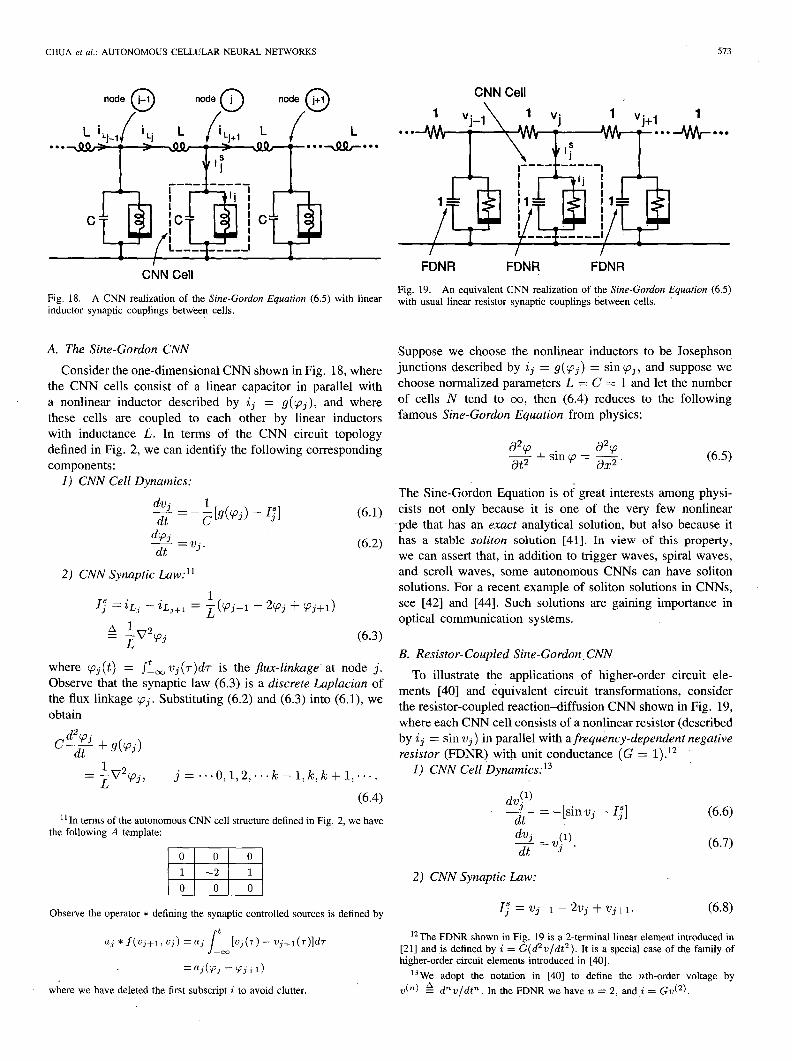
Fig. 18. A CNN realization of the Sine-Gordon Equation (6.5) with linear Fig. 19. An equivalent CNN realization of the Sine-Gordon Equation (6.5) with usual linear resistor synaptic couplings between cells.

inductor synaptic couplings between cells.

A. The Sine-Gordon CNN

Consider the one-dimensional CNN shown in Fig. 18, where the CNN cells consist of a linear capacitor in parallel with a nonlinear inductor described by ij = g(cpj), and where these cells are coupled to each other by linear inductors with inductance L. In terms of the CNN circuit topology defined in Fig. 2, we can identify the following corresponding components:

1) CNN Cell Dynamics:

d% dt

-llj.

2) CNN Synaptic Law:”

Ij” =iL, - iLj+l = $+1- 2% + cpj+d

A 1 =- L V2Pj

(6.1)

(6.2)

(6.3)

where cpj(t) = J! o. uj(~)d~ is the jlux-linkage at node j. Observe that the synaptic law (6.3) is a discrete Laplacian of the flux linkage ‘pj. Substituting (6.2) and (6.3) into (6.1), we obtain

= ;v2$9j, j = . . . 0, 1,2,. . . k - 1, k, k + 1,. . . .

(6.4) ” In terms of the autonomous CNN cell structure defined in Fig. 2, we have

the following A template:

Suppose we choose the nonlinear inductors to be Josephson junctions described by ij = g(cpj) = sin ‘pj, and suppose we choose normalized parameters L = C = 1 and let the number of cells N tend to co, then (6.4) reduces to the following famous Sine-Gordon Equation from physics:

(6.5)

The Sine-Gordon Equation is of great interests among physi- cists not only because it is one of the very few nonlinear

.pde that has an exact analytical solution, but also because it has a stable soliton solution [41]. In view of this property, we can assert that, in addition to trigger waves, spiral waves, and scroll waves, some autonomous CNNs can have soliton solutions. For a recent example of soliton solutions in CNNs, see [42] and [44]. Such solutions are gaining importance in optical communication systems.

B. Resistor-Coupled Sine-Gordon,CNN

To illustrate the applications of higher-order circuit elements [40] and equivalent circuit transformations, consider the resistor-coupled reaction-diffusion CNN shown in Fig. 19, where each CNN cell consists of a nonlinear resistor (described by ij = sin vj) in parallel with a frequency-dependent negative resistor (FDNR) with unit conductance (G = 1) .l*

1) CNN Cell Dynamics:13

d$) *= -[sin wj - Ij”]

_ v(l) dVi dt 3’

2) CNN Synaptic Law:

Observe the operator * defining the synaptic controlled sources is defined by I; = 7l-1 - 2vj + ?Jj+1. (6.8)

aj * f(UJ+l, Vj) = a] .I

t [q(T) - q+1(r)ldr “The FDNR shown in Fig. 19 is a 2-terminal linear element introduced in -cc [21] and is defined by i = G(d’v/dt’). It is a special case of the family of

=a?(% -'pj+1) higher-order circuit elements introduced in [40].

13We adopt the notation in [40] to define the nth-order voltage by where we have deleted the first subscript i to avoid clutter. vcn) k d”v/dP In the FDNR we have n = 2, and i = Gvc2).

514 IEEE TRANSACTIONS ON CIRCUITS AND SYSTEMS-I: FUNDAMENTAL THEORY AND APPLICATIONS, VOL. 42, NO. 10, OCTO,BER 1995

Substituting (6.7) and (6.8) into (6.6), and letting N + 00, we obtain again the Sine-Gordon Equation

in terms of the voltage variable V, instead of the flux-linkage variable cp in (6.5). This example shows that it is possible to obtain soliton solutions in an autonomous CNN without using inductors.

From a circuit-theoretic perspective, this example is also important because it shows that the same dynamics from a reciprocal lossless LC circuit, such as the CNN in Fig. 18, can be obtained from an active reciprocal RC circuit; such as the CNN in Fig. 19. Indeed, by using the family of higher-order circuit elements introduced in [40], an almost unlimited hiera&y of higher-order CNNs can be synthesized. The nonlinear dynamics of such high-order systems is truly mind boggling and will no doubt form an interesting and challenging fundamented subject of future research.

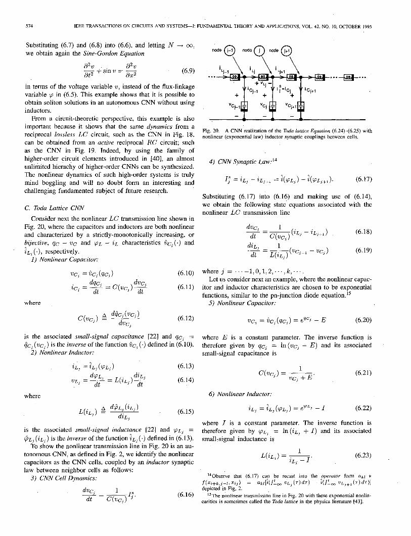
C. Toda Lattice CNN

Consider next the nonlinear LC transmission line shown in Fig. 20, where the capacitors and inductors are both nonlinear and characterized by a strictly-monotonically increasing, or bijective, qc - UC and cp~ - in characteristics &, (.) and ~~~ (.), respectively.

I) Nonlinear Capacitor:

wj = k, (qc, ) (6.10)

node 0

\

node 9 node @,

Fig. 20. A CNN realization of the Toda lattice Equation (6.24)-(6.25) with nonlinear (exponential law) inductor synaptic couplings between cells.

4) CNN Synaptic L.aw:14

I; = iLj - iLj+l = GLj) - &uj,,). (6.17)

Substituting (6.17) into (6.16) and making use of (6.14), we obtain the following state equations associated with the nonlinear LC transmission line

(6.18)

(6.19)

wherej = . ..-1.0,1,2,...,Ic;... Let us consider next an example, where the nonlinear capac-

itor and inductor characteristics are chosen to be exponential functions, similar to the pn-junction diode equation.15

5) Nonlinear Capacitor:

dqc iCj = dt

dvc 3 = C(vc,)$

where

Vcj = 8cj (qc, ) = eqcj - E (6.20)

is the associated small-signal capacitance [22] and qc, = Gc, (UC, ) is the inverse of the function 8cj (.) defined in (6.10).

2) Nonlinear Inductor:

iL3 = ;L, (CpLj) (6.13)

VL 3

where

(6.14)

(6.15)

is the associated small-signal inductance [22] and (PLY = @Lo (in,) is the inverse of the function ~~~ (.) defined in (6.13).

To show the nonlinear transmission line in Fig. 20 is an autonomous CNN, as defined in Fig. 2, we identify the nonlinear capacitors as the CNN cells, coupled by an inductor synaptic law between neighbor cells as follows:

3) CNN Cell Dynamics:

dvc, _ 1 --- dt

p C(w!,) 3’

(6.16)

where E is a constant parameter. The inverse function is therefore given by qc, = In (WC, + E) and its associated small-signal capacitance is

cw = --& (6.21) 3

6) Nonlinear Inductor:

(6.22)

where I is a constant parameter. The inverse function is therefore given by (PLY = In (in, f I) and its associated small+ignal inductance is

t40bserve that (6.17) can be recast into the operator form akl * f(G+k,j+r> G j) = %,[W, “Lj (T)dT) - WC0 Wjfl(T) dT)l depicted in Fig. 2.

15The nonlinear transmission line in Fig. 20 with these exponential nonlin- earities is sometimes called the Toda lattice in the physics literature [43].


Subsituting (6.21) and (6.23) into (6.18) and (6.19), we obtain the following well-known state equations of the Toda Lattice [43]:

% = (UC, + E)(iLj - iLj,,) (6.24)

2 = (iLj + I)(wcj-l - “C,)

wherej=~~~-1,0,1,2,~~~,Ic,~~~Itfollowsfromtheabove derivations that the Toda lattice is also an autonomous CNN.

D. Lotka-Volterra (Prey-Predator) CNN

For our last example, let us consider the Lotka-Volterra equation

d?i _ dt- X&j-l - Xj+1) j = . . . -.I,(), 1,. . . ) k, . . . .

(6.26)

Equation (6.26) is a classic equation in ecology and theoretical biology; it is usually called the Prey-predator model [26]. Our objective in this final section is to show that the Lotka- Volterra equation can be transformed into the Toda lattice equations (6.24)-(6.25) of the preceding section. Hence, the Lotka-Volterra Equation can also be studied as an autonomous CNN. To establish this equivalence, let us group the equations with odd or even indexes in (6.26) separately to obtain the following two systems of coupled equations:i6

d&j-l dt =X2j-l(X2j-2 - X2j) dXzj - = XZj(XZj-1 - X2jfl) dt

j = . . . -1,0,1,2;..,k,... . (6.28)

Equating (6.27) and (6.28) to zero, we obtain the following equilibrium points:

X2+ =X2i = E, j = . . . -l,O, 1,2, . . . ) Ic, . . . x2+1 =xq+1 = I, j=...-1,0,1,2,...,k,...

(6.29)

for arbitrary values of E and I. Let us change variables by defining

X2j k IJ~, + E A x2j-1 = iLj + I. (6.30)

Substituting (6.30) into (6.28), we obtain

% = (UC, + E)(& - iLj+J.

Similarly, substituting (6.30) into (6.27), we obtain

diLj _ - - (iL, + q(w-1 - w,).

dt

(6.31)

(6.32)

t61n a Prey-predator system, we can interpret zlj-1 as the population of prq’eys as a function of the discrete distance 2j - 1 and z2j as the population of predators as a function of the discrete distance Zj; j = . ..-l.O,l,...k,....

Observe that (6.31) and (6.32) are identical to the Toda lattice equations (6.24) and (6.25), respectively. Here, the capacitor voltage wcj can be interpreted as the variations in the population of an “even-numbered” species, (e.g., preys such as rabbits, phytoplanktons) about some equilibrium population equal to E. Similarly, the inductor current ~~~ can be interpreted as the variations of an “odd-numbered” species (e.g., predators such as foxes, planktons, etc.) about some equilibrium population equal to I.

One immediate bonus of the above identification of the Lotka-Volterra Equations (6.27)-(6.28) with the nonlinear LC transmission line of Fig. 20 is that this model represents a conservative system since the total energy is conserved in the LC transmission line. This same conclusion can be proved mathematically by exhibiting a first integral of the motion in the corresponding nonlinear reaction-diffusion pde [26]. However, this task is nontrivial and nonintuitive. In contrast, since the LC transmission line in Fig. 20 is lossless, we had obtained the same conclusion for free! This example demonstrates the value of the CNN paradigm as a unifying framework.

VII. CONCLUDING REMARKS

Although this tutorial paper focuses only on reaction- dzfhusion CNNs, it is clear from the numerous examples presented in the preceding sections that any nonlinear higher- order, (e.g., [44]), and/or time-varying (nonautonomous) system of pde’s can be simulated by a CNN by synthesizing the appropriate synaptic “lumped circuit” coupling whose continuum limits represent the associated partial derivative op- eratcii, e.g., f(t)(a4u(x, t)/ax4), (a/ay)(u(x, y)(f3”u/ax3). -, etc. Such complicated synaptic couplings can no longer be realized by layers of resistive, inductive, or capacitive grids, as in reaction-diffusion CNNs. However, by using the concepts developed in [23], [40], such complex synaptic couplings can always be realized by using nonlinear controlled sources and higher-order circuit elements. It is in fact in such applications where the higher-order circuit elements introduced in [40] will play an essential if not indispensable role.

Observe that the nonautonomous first-order CNN cell nij in Fig. 3(a) becomes autonomous for constant (dc) inputs Eij. This induces a constant current source equal to b,~oEij, which can be combined with the dc threshold current source I in Fig. 3(a) and (b). In other words, the space-invariant nonautonomous CNN widely used to date for processing static images [7] is equivalent to an autonomous CNN with a space-varying threshold current 1;j for each cell n;j. This observation is important because it transforms the static image processing problem into a bifurcation problem where the tools from nonlinear dynamics can be brought to bear.

The unifying power of the CNN paradigm can be exploited in at least two directions: engineering and nonengineering applications. For engineering applications (e.g., signal, image, and information processing, pattern recognition, artificial intel- ligence, etc.) nonconventional technology can be developed by mimicking the CNN-based operating mechanisms (e.g., hyper-


acuity) of many marvelous biological systems. For example, by studying how the electric fish manages to use its array of extremely inaccurate neurons to generate extremely accurate directional acoustical information to fence off enemies and avoid obstacles, a CNN has recently been synthesized to achieve similar “hyperacuity” performance [45].

For researchers outside of engineering, the CNN paradigm will find increasing applications in view of the large and rapidly expanding body of knowledge being generated in the CNN research community. By simply translating any such nonengineering but, CNN-based phenomenon into a corresponding CNN paradigm, many tools, results, and concepts developed for CNNs can be used to understand, explain, and control such phenomenon. For example, a CNN can be developed to model the spread of a deadly virus, or an epidemic, in a community so that effective methods for presenting a further spread to a larger area can be instituted.17 In addition to the advantage of not having to numerically solve a system of nonlinear pdes, which is generally extremely costly and time consuming,‘8 one can often manage to fine tune a CNN to better model a given situation. This approach is similar to the “breadboarding” approach used by electronic engineers to design and optimize a new electronic product. Such flexibility is a luxury that can not be achieved by working directly with a complicated system of nonlinear pdes.

But above all, by virtue of the sheet-like nature of brain tissues, where neurons are distributed along planar layers” [48], the CNN provides an ideal substrate and active medium for modeling many brain functions, including sensory information processing. Indeed, regardless of the nature of the sensory modality (visual, auditory, olfactory, taste, etc.), all such input information must be transformed by the brain and mapped into corresponding “images’‘-in view of the “sheet-like” topology of the brain. The recognition that the CNN paradigm is applicable to any setting where information is being processed as a transformed planar image has been exploited recently in the physiological modeling of the retina by [49]. Similar applications can no doubt be profitably carried out for the other sensory modalities, and eventually into mimicking the higher brain functions partially mapped out in of the recent inspiring book [48, (p. 156, Fig. 52)] . One can not help but be inspired by this awesome wiring diagram of the brain, which metaphorically resembles the layout of a massive VLSI chip. Portions of this figure could possibly be simulated by interconnections of some futuristic complex of CNN chips.

ACKNOWLEDGMENT

The authors would like to thank Chai Wah Wu, Anshan

170ne recent rather successful example of an e$‘ixtive control method used to prevent the spread of rabies in infected foxes-whose dynamics is modeled by the travelling autowave solution of a nonlinear reaction-diffusion pde--consists simply of maintaining a 14-km wide barrier of healthy foxes [46] !

‘*Digital CNN hardware acceleration boards are available for solving such problems accurately and rapidly [47]. Moreover, for applications requiring a real-time response, dedicated VLSI chips can be fabricated for this purpose.

lgThe cerebral cortex of humans consists of two separate sheets of neurons, one on each side of the head, where each sheet when unfolded is approximately the size of a large handkerchief.

Huang, and Guo-Qun Zhong for their assistance.

REFERENCES

HI

r21

r31

r41 [51

161

[71

PI

r91

1101

1111

1121

r131

u41

u51

[I61

Cl71

1181

[I91 PO1

WI

G91

~31

~41

WI

LW

~271

vu

P91

r301

[311

L. 0. Chua and L. Yang, “Cellular neural network: Theory and practice,” IEEE Trans. Circuits Syst., vol. 35, pp. 1257-1290, Oct. 1988. L. 0. Chua and T. Roska, “The CNN paradigm,” IEEE Trans. Circuits Syst. Z, vol. 40, pp. 147-156, Mar. 1993.

“The CNN universal machine: An analogic array computer,” GTrans. Circuits Syst. II, vol. 40, pp. 163-173, Mar. 1993. S. Zeki, A Vision of the Brain. Oxford: Blackwell, 1993. Special issue on cellular neural networks, ht. J. Circuit Theory Applicat., vol. 20, Sept./Ott. 1992. Suecial issue on cellular neural networks. IEEE Trans. Circuits Svst. I and II, vol. 40, Mar. 1993. T. Roska and Vandewalle, Cellular Neural Networks. New York: Wilev, 1994. Proc. Int. Workshop Cellular Neural Networks and Their Aoulicat., Bu- dapest, Hungary, Dec. 1990.

. 1

Proc. Int. Workshop Cellular Neural Networks and Their Applicat., Mu- nich, Germany, Oct. 1992. Proc. Int. Workshop Cellular Neural Networks and Their Applicat., Rome, Italy, Dec. 1994. V. Perez-Muhuzuri, V. Perez-Villar, and L. 0. Chua, “Prooaaation failure in linear arrays of Chua’s circuits,” ht. J. Bifurc. and Chaos, vol. 2, no. 2, pp. 403406, June 1992. -, “Auto-waves for image processing on a two-dimensional CNN array of excitable nonlinear circuits: Flat and wrinkled labyrinths,” IEEE Trans. Circuits Syst. Z, vol. 40, pp. 174-181, Mar. 1993. V. Perez-Villar, A. Perez-Muiiuzuri, and L. 0. Chua, “Spiral waves on a 2-D array of nonlinear circuits,” IEEE Trans. Circuits Syst. Z, vol: 40, pp. 872-877, Nov. 1993. V. Perez-Mufiuzuri, M. Gomez-Gesteira, A. Perez-Mufiuzuri, L. 0. Chua, and V. Perez-Villar, “Sidewall forcing of hexagonal Turing patterns: Rhombic patterns,” Physica, vol. D-82, pp. 195-204, Apr. 1995. A. Perez-Muiiuzuri, M. Gomez-Gesteira, L. 0. Chua, and V. Perez-Villar, “Spatiotemporal structures in discretely-coupled arrays of nonlinear circuits: A review,” Int. J. B&t-c. and Chaos, vol. 5, no. 1, pp. 17-50, Feb. 1995. I. Perez-Mariho, M. de Castro, V. Perez-Mufiuzuri, M. G6mez-Gesteira, L. 0. Chua, and V. Perez-Villar, “Study of reentry initiation in coupled parallel fibers,” IEEE Trans. Circuits Syst., vol. 42, no. 10, pp. 665-671, this issue. M. G6mez-Gesteira, V. Perez-Muhuzuri, L. 0. Chua, and V. Perez- Villar, “Coexistence of excitability, Hopf and Turing modes in a one- dimensional arrav of nonlinear circuits,” IEEE Trans. Circuits Svst. I, vol. 42, no. 10, pp. 672-677, this issue. R. Madan, Chua’s Circuit: A Paradigm for Chaos. Singapore: World Scientific, 1993. J. D. Murray, Mathematical Biology. New York: Springer:Verlag, 1989. L. 0. Chua, Introduction to Nonlinear Network Theory. New York: McGraw-Hill, 1969. L. T. Bruton, RC Active Circuits. Englewood Cliffs, NJ: Prentice-Hall, 1980. L. 0. Chua. C. A. Desoer. and E. S. Kuh. Linear and Nonlinear Circuits. New York: McGraw-Hill; 1985: L. V. Kantorovich and V. I. Krylov, Approximate Methods of Higher Analysis. New York: Interscience, 1964. J. P. Keener, “Propagation and its failure in coupled systems of discrete excitable cells,” SIAM J. Appl. Math., vol. 47, pp. 556-572, June 1987. R. A. Fisher, “The wave of advance of advantageous genes,” Ann. Eugenics, vol. 7, pp. 355-369, 1937. N. F. Britton, Reaction-Diffusion Equations and Their Applications to Biology. New York: Academic, 1986. J. Nagumo, S. Arimoto, and S. Yoshizawa, “An active pulse transmission line simulating nerve axon,” in Proc. Inst. Radio Eng., 1962, vol. 50, pp. 2061-2070. R. FitzHugh, “Mathematical models of excitation and propagation nerve,” in Biological Engineering, H. Schwan, Ed. New York: McGraw-Hill, 1969. A. L. Hodgkin and A. F. Huxley, “A quantitative description of membrane current and its application to conduction and excitation in nerve,” J. Physiology, vol. 117, pp. 500-544, 1952. J. J. Tyson, The Belousov-Zhabotinskii Reaction, Lecture Notes in Bio- mathematics, vol. 10. New York: Springer-Verlag, 1976. I. Prigogine and R. Lefever, “Symmetry breaking instabilities in dissi- pative systems, II,” J. C/rem. Phys., vol. 48, no. 4, pp. 1695-1700, Feb. 1968.


~321

t331

t341

[351

[361

I371

[381

[391

t401

;::3

t431

WI

t451

[461

[471

[481 WI

A. M. Turing, “The chemical basis of morphogenesis,” Philos. Trans. R. Sm. London, ser. B, vol. 237, pp. 31-12, 1952. H. Meinhardt, Models of Biological Pattern Formation. New York: Academic, 1982. ” - L. Goras. L. 0. Chua, and D. Leenaerts, “Turing nattems in CNNs-Part I: Once-over lightly,” IEEE Trans. Circuits Sy% I, vol. 42, no. 10, pp. 602-611, this issue. L. Goras and L. 0. Chua, “Turing patterns in CNNs-Part II: Equations and behavior,” IEEE Trans. Circuits Syst. I, vol. 42, no. 10, pp. 612-626, this issue. L. Goras, L. 0. Chua, and L. Pivka, “Turing patterns in CNNs, Part III: Computer simulation results,” IEEE Trans. Circuits Syst. I, vol. 42, no. 10, pp. 627-637, this issue. R. J. Field and R. M. Noyes, “Oscillations in chemical systems, IV. Limit cycle behavior in a model of a real chemical reaction,” J. Chem. Phys., vol. 60, pp. 1877-1884, Mar. 1974. L. 0. Chua and S. M. Kang, “Memiistive devices and systems,” Proc. IEEE, vol. 64, no. 2, pp. 209-223, Feb. 1976. L. 0. Chua, “Memristor-The missing circuit element,” IEEE Trans. Circuit Theory, vol. 18, no. 5, pp. 507-519, Sept. 1971.

“Device modeling via basic nonlinear circuit elements,” IEEE G ’Circuits Syst., vol. 27, no. 11, pp. 1014-1044, Nov. 1980. P. G. Drazin, Solitons. Cambridge: Cambridge Univ. Press, 1983. V. I. Nekorkin, V. B. Kazantsev, N. F. Rulkov, M. G. Velarde, and L. 0. Chua, “Homoclinic orbits and solitary waves in a one-dimensional array of Chua’s circuits,” IEEE Trans. Circuits Syst. I, vol. 42, no. 10, pp. 785-801, this issue. M. Toda, Theory of Nonlinear Lattices. New York: Springer-Verlag, 1981. T. Roska, L. 0. Chua, D. Wolf, T. Kozek, R. Tetzlaff, and F. Puffer, “Sim- ulating nonlinear waves and partial differential equations via CNN-Part I. Basic techniques; also T. Kozek, L. 0. Chua, T. Roska, D. Wolf, R. Tetzlaff, F. Puffer, and K. Lotz, “Part II. Typical examples,” IEEE Trans. Circuits Syst. I, vol. 42, no. 10, pp. 807-820, this issue. B. E. Shi, T. Roska, and L. 0. Chua, “Random variation in analog VLSI neural networks for linear image filtering,” in Proc. ZEEE Int. Con$ Neural Networks, 1994, vol. 3, pp. 1917-1922. A. Kallen, P. Arcuri, and J. D. Murray, “A simple model for the spatial spread and control of rabies,” J. Theoretical Biology, vol. 116, pp. 377-393, Oct. 1985. T. Roska, G. Bartfai, P. Szolgay, T. Sziranyi, A. Radvlnyi, T. Kozek, and Zs. Ugray, “A hardware accelerator board for cellular neural networks: CNN-HAC,“, in Proc. IEEE Int. Workshop Cellular Neural Networks Applicat., 1990, pp. 160-168; extended version in Znt. J. Circuit Theory and Applicat., vol. 20, pp. 589-599, Sept./Ott. 1992. F. Crick, The Astonishing Hypothesis. New York: Scribner, 1994. F. Werblin, T. Roska, and L. 0. Chua, “The analogic cellular neural network as a bionic eye,” to be published in Int. J. Circuit Theory Applicat.

Leon 0. Chua (S’60-M’62-SM’7&F’74), for a photograph and biography, see this issue, p. 558.

Martin Hasler (M’81-SM’90-F’93) received the Diploma in 1969 and the Ph.D. degree in 1973 from the Swiss Federal Institute of Technology, Zurich, both in physics.

Since 1984, he has been a Professor with the Swiss Federal Institute of Technology, Lausanne. His research interests are in the field of nonlinear circuits and systems, including neural networks. He is the author and coauthor of about 100 scientific papers and 4 books, including Nonlinear Circuits (Boston: Artech House, 1986). He is currently the

Editor of the IEEE TRANSACTIONS ON CIRCUITS AND SYSTEMS, PART I.

George S. Moschytz (M’65-SM’77-F’78) received the E.E. Diploma and Ph.D. degrees in 1962, from the Swiss Federal Institute of Technology (ETH), Zurich in 1958 and 1962, respectively.

From 1960 to 1962, he was with RCA Laborato- ries in Zurich where he worked on envelope-delay measurement techniques for the transmission of color TV signals and from 1963 to 1972 with Bell Labs in Holmdel, NJ, where he was involved in the design of hybrid-integrated active RC filters and silicon-integrated logic circuits for use in data

transmission equipment. Since 1973, he has been a Professor of network theory and signal processing and Director of the Laboratory for Signal and Information Processing at the Swiss Federal Institute of Technology (ETH), Zurich. He has authored many papers in the field of network theory, active and switched-capacitor filters and network design, and sensitivity theory and holds several patents in these areas. He is author of Linear Integrated Networks: Fundamentals (New York: Van Nostrand Reinhold, 1974), Linear Integrated Networks: Design (New York: Van Nostrand Reinhold, 1975) co-author of the Active Filter Design Handbook (London: Wiley, 1981), and editor of MOS Switched-Capacitor Fitlers: Analysis and Design (New York: IEEE Press, 1984). His present interests include signal processing, digital, switched- capacitor and adaptive filters, neural networks for signal processing, and the application of signal-processing techniques to biological signals.

Dr. Moschytz is an elected member of the Swiss Academy of Engineering Sciences, winner of Best Paper Award, and member of Eta Kappa Nu Honor Society. He is President of the IEEE Swiss Chapter on Digital Communication Systems and from 1981 to 1982, he was President of the Swiss Section of the IEEE. He is presently on the Board of Governors of the IEEE Circuits and Systems Society.

Jacques Neirynck (F’81) received the E.E. and Ph.D degrees in 1954 and 1958, respectively, both from the University of Louvain, Belgium.

After working two years for the Foraky Com- pany, from 1957 to 1963, he became Lecturer and Professor at Lovanium University in Kinshasa (Zaire). From 1963 to 1972, he worked for the Philips Research Laboratory in Brussels. He became Adjoint Director of that laboratory and Technical Director of the group working in digital simulation of integrated circuits for the Philips Company. Si-

multaneously, he was Professor at the University of Louvain. Since 1972, he has been Professor at the Swiss Federal Institute of Technology, Department of Electrical Engineering, Lausanne. His present research interests include filter design, circuit simulation, nonlinear circuit theory, and artificial neural networks. In 1991, he was among the founders of Eurecom, a French and Swiss joint venture in teaching and research, located at Sophia Antipolis and devoted to Communication Systems.

Dr. Neirynck is the editor of the Trait& d’Electricit6, an encyclopedia of electrical engineering in 22 volumes, for which he was granted the Denzler prize. In 1994, he has received the “1994 Educational Activities Board Major Educational Innovation Award” from the Institute of Electrical and Electronics Engineers (IEEE).

ieee transactions on circuits and systems-i: … · 2019-08-16 · ing paradigm for pattern...

Documents