ieee transactions on computers, vol. 60, no. 1, january

An Architecture for Fault-TolerantComputation with Stochastic Logic

Weikang Qian, Student Member, IEEE, Xin Li,

Marc D. Riedel, Member, IEEE, Kia Bazargan, and David J. Lilja, Fellow, IEEE

Abstract—Mounting concerns over variability, defects, and noise motivate a new approach for digital circuitry: stochastic logic, that is

to say, logic that operates on probabilistic signals and so can cope with errors and uncertainty. Techniques for probabilistic analysis of

circuits and systems are well established. We advocate a strategy for synthesis. In prior work, we described a methodology for

synthesizing stochastic logic, that is to say logic that operates on probabilistic bit streams. In this paper, we apply the concept of

stochastic logic to a reconfigurable architecture that implements processing operations on a datapath. We analyze cost as well as the

sources of error: approximation, quantization, and random fluctuations. We study the effectiveness of the architecture on a collection of

benchmarks for image processing. The stochastic architecture requires less area than conventional hardware implementations.

Moreover, it is much more tolerant of soft errors (bit flips) than these deterministic implementations. This fault tolerance scales

gracefully to very large numbers of errors.

Index Terms—Stochastic logic, reconfigurable hardware, fault-tolerant computation.

Ç

1 INTRODUCTION

THE successful design paradigm for integrated circuitshas been rigidly hierarchical, with sharp boundaries

between different levels of abstraction. From the logic levelup, the precise Boolean functionality of the system is fixedand deterministic. This abstraction is costly: variability anduncertainty at the circuit level must be compensated for bybetter physical design. With increased scaling of semicon-ductor devices, soft errors caused by ionizing radiation area major concern, particularly for circuits operating in harshenvironments such as space. Existing methods mitigateagainst bit-flips with system-level techniques like error-correcting codes and modular redundancy.

Randomness, however, is a valuable resource in computa-tion. A broad class of algorithms in areas such as crypto-graphy and communication can be formulated with lowercomplexity if physical sources of randomness are available[1], [2]. Applications that entail the simulation of randomphysical phenomena, such as computational biology andquantum physics, also hinge upon randomness (or goodpseudorandomness) [3].

We advocate a novel view for computation, calledstochastic logic. Instead of designing circuits that transformdefinite inputs into definite outputs—say Boolean, integer, orfloating-point values into the same—we synthesize circuitsthat conceptually transform probability values into prob-ability values. The approach is applicable for randomizedalgorithms. It is also applicable for data intensive applicationssuch as signal processing where small fluctuations can betolerated but large errors are catastrophic. In such contexts,

our approach offers savings in computational resources andprovides significantly better fault tolerance.

1.1 Stochastic Logic

In prior work, we described a methodology for synthesizingstochastic logic [4]. Operations at the logic level areperformed on randomized values in serial streams or onparallel “bundles” of wires. When serially streaming, thesignals are probabilistic in time, as illustrated in Fig. 1a; inparallel, they are probabilistic in space, as illustrated in Fig. 1b.

The bit streams or wire bundles are digital, carrying zerosand ones; they are processed by ordinary logic gates, such asAND and OR. However, the signal is conveyed through thestatistical distribution of the logical values. With physicaluncertainty, the fractional numbers correspond to theprobability of occurrence of a logical one versus a logicalzero. In this way, computations in the deterministic Booleandomain are transformed into probabilistic computations inthe real domain. In the serial representation, a real number xin the unit interval (i.e., 0 � x � 1) corresponds to a bitstream XðtÞ of length N , t ¼ 1; 2; . . . ; N . In the parallelrepresentation, it corresponds to the bits on a bundle ofN wires. The probability that each bit in the stream or on thebundle is one is P ðX ¼ 1Þ ¼ x.

Throughout this paper, we illustrate our method withserial bit streams. However, our approach is equallyapplicable to parallel wire bundles. Indeed, we haveadvocated stochastic logic as a framework for synthesis oftechnologies such as nanowire crossbar arrays [5].

Our synthesis strategy is to cast logical computations asarithmetic operations in the probabilistic domain andimplement these directly as stochastic operations on data-paths. Two simple arithmetic operations—multiplicationand scaled addition—are illustrated in Fig. 2.

. Multiplication. Consider a two-input AND gate,shown in Fig. 2a. Suppose that its inputs are two

IEEE TRANSACTIONS ON COMPUTERS, VOL. 60, NO. 1, JANUARY 2011 93

. The authors are with the Department of Electrical and ComputerEngineering, University of Minnesota, 200 Union St. S.E., Minneapolis,MN 55455. E-mail: {qianx030, lixxx914, mriedel, kia, lilja}@umn.edu.

Manuscript received 4 Feb. 2010; revised 2 July 2010; accepted 24 Aug. 2010;published online 23 Sept. 2010.For information on obtaining reprints of this article, please send e-mail to:[email protected], and reference IEEECS Log Number TCSI-2010-02-0087.Digital Object Identifier no. 10.1109/TC.2010.202.

0018-9340/11/$26.00 � 2011 IEEE Published by the IEEE Computer Society

independent bit streams X1 and X2. Its output is abit stream Y , where

y ¼ P ðY ¼ 1Þ ¼ P ðX1 ¼ 1 and X2 ¼ 1Þ¼ P ðX1 ¼ 1ÞP ðX2 ¼ 1Þ ¼ x1x2:

Thus, the AND gate computes the product of the

two input probability values.. Scaled Addition. Consider a two-input multiplexer,

shown in Fig. 2b. Suppose that its inputs are twoindependent stochastic bit streams X1 and X2 and itsselecting input is a stochastic bit stream S. Its outputis a bit stream Y , where

y ¼ P ðY ¼ 1Þ¼ P ðS ¼ 1ÞP ðX1 ¼ 1Þ þ P ðS ¼ 0ÞP ðX2 ¼ 1Þ¼ sx1 þ ð1� sÞx2:

(Note that throughout the paper, multiplication and

addition represent arithmetic operations, not Boolean

AND and OR.) Thus, the multiplexer computes the

scaled addition of the two input probability values.

More complex functions such as division, the Taylor

expansion of the exponential function, and the square root

function can also be implemented with only a dozen or so

gates each using the stochastic methodology. Prior work

established specific constructs for such operations [6], [7],

[8]. We tackle the problem more broadly: we propose a

synthesis methodology for stochastic computation.The stochastic approach offers the advantage that

complex operations can be performed with very simple

logic. Of course, the method entails redundancy in the

encoding of signal values. Signal values are fractional

values corresponding to the probability of logical one. If the

resolution of a computation is required to be 2�M , then the

length or width of the bit stream should be 2M bits. This is a

significant trade-off in time (for a serial encoding) or inspace (for a parallel encoding).

1.2 Fault Tolerance

The advantage of the stochastic architecture in terms ofresources is that it tolerates faults gracefully. Compare astochastic encoding to a standard binary radix encoding,say with M bits representing fractional values between 0and 1. Suppose that the environment is noisy; bit flipsoccur and these afflict all the bits with equal probability.With a binary radix encoding, suppose that the mostsignificant bit of the data gets flipped. This causesa relative error of 2M�1=2M ¼ 1=2. In contrast, with astochastic encoding, the data are represented as thefractional weight on a bit stream of length 2M . Thus, asingle bit flip only changes the input value by 1=2M ,which is small in comparison.

Fig. 3 illustrates the fault tolerance that our approachprovides. The circuit in Fig. 3a is a stochastic implementa-tion while the circuit in Fig. 3b is a conventionalimplementation. Both circuits compute the function:

y ¼ x1x2sþ x3ð1� sÞ:

Consider the stochastic implementation. Suppose that theinputs are x1 ¼ 4=8, x2 ¼ 6=8, x3 ¼ 7=8, and s ¼ 2=8. Thecorresponding bit streams are shown above the wires.Suppose that the environment is noisy and bit flips occur ata rate of 10 percent; this will result in approximately three bitflips for the stream lengths shown. A random choice of threebit flips is shown in Fig. 3a. The modified streams are shownbelow the wires. With these bit flips, the output valuechanges but by a relatively small amount: from 6=8 to 5=8.

In contrast, Fig. 3b shows a conventional implementationof the function with multiplication and addition modulesoperating on a binary radix representation: the real numbersx1 ¼ 4=8, x2 ¼ 6=8, x3 ¼ 7=8, and s ¼ 2=8 are encoded as

94 IEEE TRANSACTIONS ON COMPUTERS, VOL. 60, NO. 1, JANUARY 2011

Fig. 2. Stochastic implementation of arithmetic operations: (a) Multiplication; (b) Scaled addition.

Fig. 1. Stochastic encoding: (a) A stochastic bit stream; (b) A stochastic wire bundle. A real value x in ½0; 1� is represented as a bit stream or abundle X. For each bit in the bit stream or bundle, the probability that it is 1 is P ðX ¼ 1Þ ¼ x.

ð0:100Þ2, ð0:110Þ2, ð0:111Þ2, and ð0:010Þ2, respectively. Thecorrect result is y ¼ ð0:110Þ2, which equals 6=8. In the samesituation as above, with a 10 percent rate of bit flips,approximately one bit will get flipped. Suppose that,unfortunately, this is the most significant bit of x3. As aresult, x3 changes to ð0:011Þ2 ¼ 3=8 and the output y becomesð0:0112Þ ¼ 3=8. This is a much larger error than we expectwith the stochastic implementation.

1.3 Related Work and Context

The topic of computing reliably with unreliable componentsdates back to von Neumann and Shannon [9], [10].Techniques such as modular redundancy and majorityvoting are widely used for fault tolerance. Error correctingcodes are applied for memory subsystems and communica-tion links, both on-chip and off-chip.

Probabilistic methods are ubiquitous in circuit andsystem design. Generally, they are applied with the aimof characterizing uncertainty. For instance, statistical timinganalysis is used to obtain tighter performance bounds [11]and also applied in transistor sizing to maximize yield [12].Many flavors of probabilistic design have been proposed forintegrated circuits. For instance, [13] presents a designmethodology based on Markov random fields gearedtoward nanotechnology; [14] presents a methodology basedon probabilistic CMOS, with a focus on energy efficiency.

There has a promising recent effort to design so-calledstochastic processors [15]. The strategy in that work is to

deliberately underdesign the hardware, such that it isallowed to produce errors, and to implement error tolerancethrough software mechanisms. As much as possible, theburden of error tolerance is pushed all the way to theapplication layer. The approach permits aggressive powerreduction in the hardware design. It is particularly suitablefor high-performance computing applications, such asMonte Carlo simulations, that naturally tolerate errors.

On the one hand, our work is more narrowly circum-scribed: we present a specific architectural design fordatapath computations. On the other hand, our contributionis a significant departure from existing methods, predicatedon a new logic-level synthesis methodology. We designprocessing modules that compute in terms of statisticaldistributions. The modules process serial or parallel streamsthat are random at the bit level. In the aggregate, thecomputation is robust and accurate since the results dependonly on the statistics and not on specific bit values. Thecomputation is “analog” in character, cast in terms of real-valued probabilities, but it is implemented with digitalcomponents. The strategy is orthogonal to specific hard-ware-based methods for error tolerance, such as error-coding of memory subsystems [16]. It is also compatiblewith application layer and other software-based methodsfor error tolerance.

In [4], we presented a methodology for synthesizingarbitrary polynomial functions with stochastic logic. Wealso extended the method to the computation of arbitrary

QIAN ET AL.: AN ARCHITECTURE FOR FAULT-TOLERANT COMPUTATION WITH STOCHASTIC LOGIC 95

Fig. 3. A comparison of the fault tolerance of stochastic logic to that of conventional logic. The original bit sequence is shown above eachwire. A bit flip is indicated with a solid rectangle. The modified bit sequence resulting from the bit flip is shown below each wire andindicated with a dotted rectangle. (a) Stochastic implementation of the function y ¼ x1x2sþ x3ð1� sÞ. (b) Conventional implementation of thefunction y ¼ x1x2sþ x3ð1� sÞ, using binary radix multiplier, adder, and subtractor units.

continuous functions through nonpolynomial approxima-tions [17]. In [18], we considered the complementaryproblem of generating probabilistic signals for stochasticcomputation. We described a method for transformingarbitrary sources of randomness into the requisite prob-ability values, entirely through combinational logic.

1.4 Overview

In this paper, we apply the concept of stochastic logic to areconfigurable architecture that implements processingoperations on a datapath. We analyze cost as well as thesources of error: approximation, quantization, and randomfluctuations. We study the effectiveness of the architectureon a collection of benchmarks for image processing. Thestochastic architecture requires less area than conventionalhardware implementations. Moreover, it is much moretolerant of soft errors (bit flips) than these deterministicimplementations. This fault tolerance scales gracefully tovery large numbers of errors.

The rest of the paper is structured as follows: Section 2discusses the synthesis of stochastic logic. Section 3 presentsour reconfigurable architecture. Section 4 analyzes thesources of error in stochastic computation. Section 5describes our implementation of the architecture. Section 6provides experimental results. Section 7 presents conclu-sions and future directions of research.

2 SYNTHESIZING STOCHASTIC LOGIC

2.1 Synthesizing Polynomials

By definition, the computation of polynomial functionsentails multiplications and additions. These can be im-plemented with the stochastic constructs described inSection 1.1. However, the method fails for polynomialswith coefficients less than zero or greater than one, e.g.,1:2x� 1:2x2, since we cannot represent such coefficientswith stochastic bit streams.

In [4], we proposed a method for implementing arbitrarypolynomials, including those with coefficients less thanzero or greater than one. As long as the polynomial mapsvalues from the unit interval to values in the unit interval,then no matter how large the coefficients are, we cansynthesize stochastic logic that implements it. The proce-dure begins by transforming a power-form polynomial intoa Bernstein polynomial [19]. A Bernstein polynomial ofdegree n is of the form

BðxÞ ¼Xni¼0

biBi;nðxÞ; ð1Þ

where each real number bi is a coefficient, called a Bernsteincoefficient, and each Bi;nðxÞði ¼ 0; 1; . . . ; nÞ is a Bernsteinbasis polynomial of the form

Bi;nðxÞ ¼n

i

� �xið1� xÞn�i: ð2Þ

A power-form polynomial of degree n can be transformedinto a Bernstein polynomial of degree not less than n.Moreover, if a power-form polynomial maps the unitinterval onto itself, we can convert it into a Bernsteinpolynomial with coefficients that are all in the unit interval.

A Bernstein polynomial with all coefficients in the unitinterval can be implemented stochastically by a generalizedmultiplexing circuit, shown in Fig. 4. The circuit consists ofan adder block and a multiplexer block. The inputs to theadder are an input set fx1; . . . ; xng. The data inputs tothe multiplexer are z0; . . . ; zn. The outputs of the adder arethe selecting inputs to the multiplexer block. Thus, theoutput of the multiplexer y is set to be zi (0 � i � n), where iequals the binary number computed by the adder; this is thenumber of ones in the input set fx1; . . . ; xng.

The stochastic input bit streams are set as follows:

. The inputs x1; . . . ; xn are independent stochastic bitstreams X1; . . . ; Xn representing the probabilitiesP ðXi ¼ 1Þ ¼ x 2 ½0; 1�, for 1 � i � n.

. The inputs z0; . . . ; zn are independent stochastic bitstreams Z0; . . . ; Zn representing the probabilitiesP ðZi ¼ 1Þ ¼ bi 2 ½0; 1�, for 0 � i � n, where the bi’sare the Bernstein coefficients.

The output of the circuit is a stochastic bit stream Y inwhich the probability of a bit being one equals the Bernsteinpolynomial BðxÞ ¼

Pni¼0 biBi;nðxÞ. We discuss generating

and interpreting such input and output bit streams inSections 3.2 and 3.3.

Example 1. The polynomial f1ðxÞ ¼ 14þ 9

8 x� 158 x

2 þ 54x

3

maps the unit interval onto itself. It can be convertedinto a Bernstein polynomial of degree 3:

f1ðxÞ ¼2

8B0;3ðxÞ þ

5

8B1;3ðxÞ þ

3

8B2;3ðxÞ þ

6

8B3;3ðxÞ:

Notice that all the coefficients are in the unit interval. Thestochastic logic that implements this Bernstein polynomialis shown in Fig. 5. Assume that the original polynomial isevaluated at x ¼ 0:5. The stochastic bit streams of inputsx1, x2, and x3 are independent and each represents theprobability value x ¼ 0:5. The stochastic bit streams ofinputs z0; . . . ; z3 represent probabilities b0 ¼ 2

8 , b1 ¼ 58 ,

b2 ¼ 38 , and b3 ¼ 6

8 . As expected, the stochastic logiccomputes the correct output value: f1ð0:5Þ ¼ 0:5.

2.2 Synthesizing Nonpolynomial Functions

It was proved in [4] that stochastic logic can onlyimplement polynomial functions. In real applications, ofcourse, we often encounter nonpolynomial functions, suchas trigonometric functions. A method was proposed in [17]to synthesize arbitrary functions by approximating themvia Bernstein polynomial. Indeed, given a continuousfunction fðxÞ of degree n as the target, a set of real


Fig. 4. A generalized multiplexing circuit implementing the Bernsteinpolynomial y ¼ BðxÞ ¼

Pni¼0 biBi;nðxÞ with 0 � bi � 1, for i ¼ 0; 1; . . . ; n.

coefficients b0; b1; . . . ; bn in the interval ½0; 1� is sought tominimize the objective function

Z 1

0

fðxÞ �Xni¼0

biBi;nðxÞ !2

dx: ð3Þ

By expanding (3), an equivalent objective function canbe obtained:

fðbbÞ ¼ 1

2bbTHHbbþ ccT bb; ð4Þ

where

bb ¼ ½b0; . . . ; bn�T ;

cc ¼ �Z 1

0

fðxÞB0;nðxÞ dx; . . . ;�Z 1

0

fðxÞBn;nðxÞ dx

� �T;

HH ¼

R 10 B0;nðxÞB0;nðxÞ dx . . .

R 10 B0;nðxÞBn;nðxÞ dxR 1

0 B1;nðxÞB0;nðxÞ dx . . .R 1

0 B1;nðxÞBn;nðxÞ dx

..

. . .. ..

.R 10 Bn;nðxÞB0;nðxÞ dx . . .

R 10 Bn;nðxÞBn;nðxÞ dx

2666664

3777775:

This optimization problem is, in fact, a constrainedquadratic programming problem. Its solution can beobtained using standard techniques. Once we obtainthe requisite Bernstein coefficients, we can implement thepolynomial approximation as a Bernstein computation withthe generalized multiplexing circuit described in Section 2.1.

Example 2 (Gamma Correction). The gamma correctionfunction is a nonlinear operation used to code and decodeluminance and tristimulus values in video and still-imagesystems. It is defined by a power-law expression

Vout ¼ V�

in;

where Vin is normalized between zero and one [20]. Weapply a value of � ¼ 0:45, which is the value used inmost TV cameras.

Consider the nonpolynomial function

f2ðxÞ ¼ x0:45:

We approximate this function by a Bernstein polynomialof degree 6. By solving the constrained quadratic optimi-zation problem, we obtain the Bernstein coefficients:

b0 ¼ 0:0955; b1 ¼ 0:7207; b2 ¼ 0:3476; b3 ¼ 0:9988;

b4 ¼ 0:7017; b5 ¼ 0:9695; b6 ¼ 0:9939:

In a strict mathematical sense, stochastic logic can onlyimplement functions that map the unit interval into theunit interval. However, with scaling, stochastic logic canimplement functions that map any finite interval into anyfinite interval. For example, the functions used in grayscaleimage processing are defined on the interval ½0; 255� withthe same output range. If we want to implement such afunction y ¼ fðtÞ, we can instead implement the functiony ¼ gðtÞ ¼ 1

256 fð256tÞ. Note that the new function gðtÞ isdefined on the unit interval and its output is also on theunit interval.

3 THE STOCHASTIC ARCHITECTURE

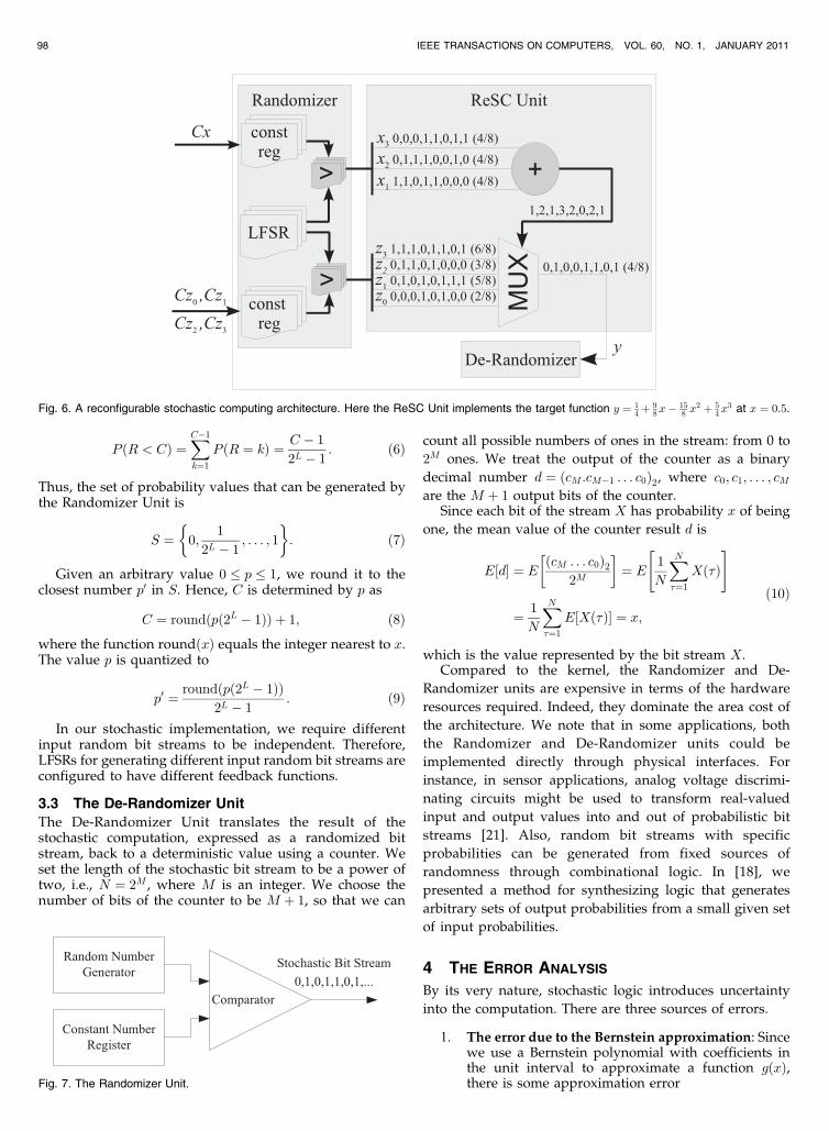
We present a novel Reconfigurable architecture based onStochastic logiC: the ReSC architecture. As illustrated inFig. 6, it is composed of three parts: the Randomizer Unitgenerates stochastic bit streams; the ReSC Unit processesthese bit streams; and the De-Randomizer Unit converts theresulting bit streams to output values. The architecture isreconfigurable in the sense that it can be used to computedifferent functions by setting appropriate values ofconstant registers.

3.1 The ReSC Unit

The ReSC Unit is the kernel of the architecture. It is thegeneralized multiplexing circuit described in Section 2.1,which implements Bernstein polynomials with coefficientsin the unit interval. As described in Section 2.2, we can useit to approximate arbitrary continuous functions.

The probability x of the independent stochastic bitstreams xi is controlled by the binary number Cx in aconstant register, as illustrated in Fig. 6. The constantregister is a part of the Randomizer Unit, discussed below.Similarly, stochastic bit streams z0; . . . ; zn representing aspecified set of coefficients can be produced by configuringthe binary numbers Czi ’s in constant registers.

3.2 The Randomizer Unit

The Randomizer Unit is shown in Fig. 7. To generate astochastic bit stream, a random number generator producesa number R in each clock cycle. If R is strictly less than thenumber C stored in the corresponding constant numberregister, then the comparator generates a one; otherwise, itgenerates a zero.

In our implementation, we use linear feedback shiftregisters (LFSRs). Assume that an LFSR has L bits.Accordingly, it generates repeating pseudorandom num-bers with a period of 2L � 1. We choose L so that2L � 1 � N , where N is the length of the input random bitstream. This guarantees good randomness of the input bitstreams. The set of random numbers that can be generatedby such an LFSR is f1; 2; . . . ; 2L � 1g, and the probabilitythat R equals a specific k in the set is

P ðR ¼ kÞ ¼ 1

2L � 1: ð5Þ

Given a constant integer 1 � C � 2L, the comparatorgenerates a one with probability


Fig. 5. Stochastic logic implementing the Bernstein polynomial f1ðxÞ ¼28B0;3ðxÞ þ 5

8B1;3ðxÞ þ 38B2;3ðxÞ þ 6

8B3;3ðxÞ at x ¼ 0:5. Stochastic bitstreams x1; x2, and x3 encode the value x ¼ 0:5. Stochastic bit streamsz0; z1; z2, and z3 encode the corresponding Bernstein coefficients.

P ðR < CÞ ¼XC�1

k¼1

P ðR ¼ kÞ ¼ C � 1

2L � 1: ð6Þ

Thus, the set of probability values that can be generated bythe Randomizer Unit is

S ¼ 0;1

2L � 1; . . . ; 1

� �: ð7Þ

Given an arbitrary value 0 � p � 1, we round it to theclosest number p0 in S. Hence, C is determined by p as

C ¼ roundðpð2L � 1ÞÞ þ 1; ð8Þwhere the function roundðxÞ equals the integer nearest to x.The value p is quantized to

p0 ¼ roundðpð2L � 1ÞÞ2L � 1

: ð9Þ

In our stochastic implementation, we require differentinput random bit streams to be independent. Therefore,LFSRs for generating different input random bit streams areconfigured to have different feedback functions.

3.3 The De-Randomizer Unit

The De-Randomizer Unit translates the result of thestochastic computation, expressed as a randomized bitstream, back to a deterministic value using a counter. Weset the length of the stochastic bit stream to be a power oftwo, i.e., N ¼ 2M , where M is an integer. We choose thenumber of bits of the counter to be M þ 1, so that we can

count all possible numbers of ones in the stream: from 0 to

2M ones. We treat the output of the counter as a binary

decimal number d ¼ ðcM:cM�1 . . . c0Þ2, where c0; c1; . . . ; cMare the M þ 1 output bits of the counter.

Since each bit of the stream X has probability x of being

one, the mean value of the counter result d is

E½d� ¼ E ðcM . . . c0Þ22M

� �¼ E 1

N

XN�¼1

Xð�Þ" #

¼ 1

N

XN�¼1

E½Xð�Þ� ¼ x;ð10Þ

which is the value represented by the bit stream X.Compared to the kernel, the Randomizer and De-

Randomizer units are expensive in terms of the hardware

resources required. Indeed, they dominate the area cost of

the architecture. We note that in some applications, both

the Randomizer and De-Randomizer units could be

implemented directly through physical interfaces. For

instance, in sensor applications, analog voltage discrimi-

nating circuits might be used to transform real-valued

input and output values into and out of probabilistic bit

streams [21]. Also, random bit streams with specific

probabilities can be generated from fixed sources of

randomness through combinational logic. In [18], we

presented a method for synthesizing logic that generates

arbitrary sets of output probabilities from a small given set

of input probabilities.

4 THE ERROR ANALYSIS

By its very nature, stochastic logic introduces uncertainty

into the computation. There are three sources of errors.

1. The error due to the Bernstein approximation: Sincewe use a Bernstein polynomial with coefficients inthe unit interval to approximate a function gðxÞ,there is some approximation error


Fig. 6. A reconfigurable stochastic computing architecture. Here the ReSC Unit implements the target function y ¼ 14þ 9

8x� 158 x

2 þ 54 x

3 at x ¼ 0:5.

Fig. 7. The Randomizer Unit.

e1 ¼ gðxÞ �Xni¼0

bi;nBi;nðxÞ��

��: ð11Þ

We could use the L2-norm to measure theaverage error as

e1avg ¼1

1� 0

Z 1

0

gðxÞ �Xni¼0

bi;nBi;nðxÞ !2

dx

0@

1A

0:5

¼Z 1

0

gðxÞ �Xni¼0

bi;nBi;nðxÞ !2

dx

0@

1A0:5

:

ð12ÞThe average approximation error e1avg only

depends on the original function gðxÞ and the degreeof the Bernstein polynomial; e1avg decreases as nincreases. For all of the functions that we tested, aBernstein approximation of degree of 6 was suffi-cient to reduce e1avg to below 10�3.1

2. The quantization error: As shown in Section 3.2,given an arbitrary value 0 � p � 1, we round it to theclosest number p0 in S ¼ f0; 1

2L�1 ; . . . ; 1g and generatethe corresponding bit stream. Thus, the quantizationerror for p is

jp� p0j � 1

2ð2L � 1Þ ; ð13Þ

where L is the number of bits of the LFSR.Due to the effect of quantization, we will

computePn

i¼0 b0i;nBi;nðx0Þ instead of the Bernstein

approximationPn

i¼0 bi;nBi;nðxÞ, where b0i;n and x0

are the closest numbers to bi;n and x, respectively,in set S. Thus, the quantization error is

e2 ¼Xni¼0

b0i;nBi;nðx0Þ �Xni¼0

bi;nBi;nðxÞ��

��: ð14Þ

Define �bi;n ¼ b0i;n � bi;n and �x ¼ x0 � x. Then,using a first order approximation, the error due toquantization is

e2 �Xni¼0

Bi;nðxÞ�bi;n þXni¼0

bi;ndBi;nðxÞ

dx�x

��

¼Xni¼0

Bi;nðxÞ�bi;n þ nXn�1

i¼0

ðbiþ1;n � bi;nÞBi;n�1ðxÞ�x��

��:Notice that since 0 � bi;n � 1, we have jbiþ1;n �

bi;nj � 1. Combining this with the fact thatPni¼0 Bi;nðxÞ ¼ 1 and j�bi;nj; j�xj � 1

2ð2L�1Þ , we have

e2 �1

2ð2L � 1ÞXni¼0

Bi;nðxÞ��

��þ n

2ð2L � 1ÞXn�1

i¼0

Bi;n�1ðxÞ��

�� ¼ nþ 1

2ð2L � 1Þ :ð15Þ

Thus, the quantization error is inversely propor-tional to 2L. We can mitigate this error by increasingthe number of bits L of the LFSR.

3. The error due to random fluctuations: Due to theBernstein approximation and the quantization effect,the output bit stream Y ð�Þ ð� ¼ 1; 2; . . . ; NÞ hasprobability p0 ¼

Pni¼0 b

0i;nBi;nðx0Þ that each bit is

one. The De-Randomizer Unit returns the result

y ¼ 1

N

XN�¼1

Y ð�Þ: ð16Þ

It is easily seen that E½y� ¼ p0. However, therealization of y is not, in general, exactly equal top0. The error can be measured by the variation as

V ar½y� ¼ V ar 1

N

XN�¼1

Y ð�Þ" #

¼ 1

N2

XN�¼1

V ar½Y ð�Þ�

¼ p0ð1� p0ÞN

:

ð17Þ

Since V ar½y� ¼ E½ðy� E½y�Þ2� ¼ E½ðy� p0Þ2�, the errordue to random fluctuations is

e3 ¼ jy� p0j �ffiffiffiffiffiffiffiffiffiffiffiffiffiffiffiffiffiffiffiffip0ð1� p0Þ

N

r: ð18Þ

Thus, the error due to random fluctuations isinversely proportional to

ffiffiffiffiffiNp

. Increasing the lengthof the bit stream will decrease the error.

The overall error is bounded by the sum of the abovethree error components:

e ¼ jgðxÞ � yj � gðxÞ �Xni¼0

bi;nBi;nðxÞ��

��þXni¼0

bi;nBi;nðxÞ �Xni¼0

b0i;nBi;nðx0Þ��

��þXni¼0

b0i;nBi;nðx0Þ � y��

��¼ e1 þ e2 þ e3:

ð19Þ

Note that we choose the number of bits L of the LFSRs tosatisfy 2L � 1 � N in order to get nonrepeating random bitstreams. Therefore, we have

1

2L<

1

N� 1ffiffiffiffiffi

Np :

Combining the above equation with (15) and (18), we cansee that in our implementation, the error due to randomfluctuations will dominate the quantization error. There-fore, the overall error e is approximately bounded by thesum of errors e1 and e3, i.e.,

e � e1 þ e3:

5 IMPLEMENTATION

The top-level block diagram of the system is illustrated inFig. 8. A MicroBlaze 32-bit soft RISC processor core is used


1. For many applications, 10�3 would be considered a low error rate.As discussed in Section 6, due to inherent stochastic variation, ourstochastic implementation has larger output errors than conventionalimplementations when the input error rate is low. Thus, our systemtargets noisy environments with relatively high input error rates—gen-erally, larger than 0.01.

as the main processor. Our ReSC is configured as acoprocessor, handled by the MicroBlaze. The MicroBlazetalks to the ReSC unit through a Fast Simplex Link (FSL), anFIFO-style connection bus system [22]. (The MicroBlaze isthe master; the ReSC unit is the slave.)

Consider the example of the gamma function, discussedin Example 2. We approximate this function by a Bernsteinpolynomial of degree 6 with coefficients:

b0 ¼ 0:0955; b1 ¼ 0:7207; b2 ¼ 0:3476; b3 ¼ 0:9988;

b4 ¼ 0:7017; b5 ¼ 0:9695; b6 ¼ 0:9939:

In our implementation, the LFSR has 10 bits. Thus, by (8),the numbers that we load into the constant coefficientregisters are:

C0 ¼ 99; C1 ¼ 738; C2 ¼ 357; C3 ¼ 1;023;

C4 ¼ 719; C5 ¼ 993; C6 ¼ 1;018:

Fig. 9 illustrates how we specify C code to implement thegamma correction function on the ReSC architecture. Suchcode is compiled by the MicroBlaze C compiler. Thecoefficients for the Bernstein computation are specified in

lines 4-7. These are loaded into registers in lines 9-12. Astochastic bit stream is defined in lines 14-19. Thecomputation is executed on the ReSC coprocessor in line22. The results are read in line 25.

6 EXPERIMENTAL RESULTS

We demonstrate the effectiveness of our method on acollection of benchmarks for image processing. We discussone of these, the gamma correction function, in detail. Then,we study the hardware cost and robustness of ourarchitecture on all the test cases.

6.1 A Case Study: Gamma Correction

We continue with our running example, the gammacorrection function of Example 2. We present an erroranalysis and a hardware cost comparison for this function.

6.1.1 Error Analysis

Consider the three error components described in Section 4.

1. The error due to the Bernstein approximation.Fig. 10 plots the error due to the Bernstein approx-imation versus the degree of the approximation. Theerror is measured by (12). It obviously shows that theerror decreases as the degree of the Bernsteinapproximation increases. For a choice of degreen ¼ 6, the error is approximately 4 � 10�3.

To get more insight into how the error due to theBernstein approximation changes with increasingdegrees, we apply the degree 3, 4, 5, and 6 Bernsteinapproximations of the gamma correction function toan image. The resulting images for different degreesof Bernstein approximation are shown in Fig. 13.

2. The quantization error. Fig. 11 plots the quantiza-tion error versus the number of bits L of the LFSR. Inthe figure, the x-axis is 1=2L, where the range of L isfrom 5 to 11. For different values of L; b0i and x0 in(14) change according to (9). The quantization erroris measured by (14) with the Bernstein polynomialchosen as the degree-6 Bernstein polynomial ap-proximation of the gamma correction function. Foreach value of L, we evaluate the quantization erroron 11 sample points x ¼ 0; 0:1; . . . ; 0:9; 1. The mean,the mean plus the standard deviation, and the meanminus the standard deviation of the errors areplotted by a circle, a downward-pointing triangle,and an upward-pointing triangle, respectively.


Fig. 8. Overview of the architecture of the ReSC system.

Fig. 9. C code fragments for the gamma correction function, fðxÞ ¼ x0:45,on the ReSC architecture.

Fig. 10. The Bernstein approximation error versus the degree of theBernstein approximation.

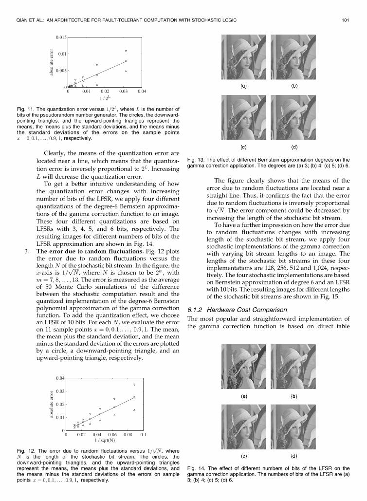
Clearly, the means of the quantization error are

located near a line, which means that the quantiza-

tion error is inversely proportional to 2L. Increasing

L will decrease the quantization error.To get a better intuitive understanding of how

the quantization error changes with increasingnumber of bits of the LFSR, we apply four differentquantizations of the degree-6 Bernstein approxima-tions of the gamma correction function to an image.These four different quantizations are based onLFSRs with 3, 4, 5, and 6 bits, respectively. Theresulting images for different numbers of bits of theLFSR approximation are shown in Fig. 14.

3. The error due to random fluctuations. Fig. 12 plotsthe error due to random fluctuations versus thelengthN of the stochastic bit stream. In the figure, thex-axis is 1=

ffiffiffiffiffiNp

, where N is chosen to be 2m, withm ¼ 7; 8; . . . ; 13. The error is measured as the averageof 50 Monte Carlo simulations of the differencebetween the stochastic computation result and thequantized implementation of the degree-6 Bernsteinpolynomial approximation of the gamma correctionfunction. To add the quantization effect, we choosean LFSR of 10 bits. For each N , we evaluate the erroron 11 sample points x ¼ 0; 0:1; . . . ; 0:9; 1. The mean,the mean plus the standard deviation, and the meanminus the standard deviation of the errors are plottedby a circle, a downward-pointing triangle, and anupward-pointing triangle, respectively.

The figure clearly shows that the means of theerror due to random fluctuations are located near astraight line. Thus, it confirms the fact that the errordue to random fluctuations is inversely proportionalto

ffiffiffiffiffiNp

. The error component could be decreased byincreasing the length of the stochastic bit stream.

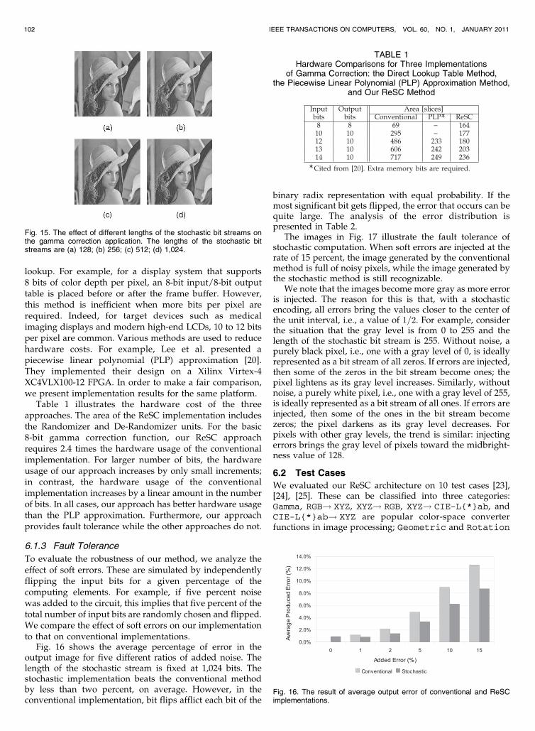
To have a further impression on how the error dueto random fluctuations changes with increasinglength of the stochastic bit stream, we apply fourstochastic implementations of the gamma correctionwith varying bit stream lengths to an image. Thelengths of the stochastic bit streams in these fourimplementations are 128, 256, 512 and 1,024, respec-tively. The four stochastic implementations are basedon Bernstein approximation of degree 6 and an LFSRwith 10 bits. The resulting images for different lengthsof the stochastic bit streams are shown in Fig. 15.

6.1.2 Hardware Cost Comparison

The most popular and straightforward implementation ofthe gamma correction function is based on direct table


Fig. 11. The quantization error versus 1=2L, where L is the number ofbits of the pseudorandom number generator. The circles, the downward-pointing triangles, and the upward-pointing triangles represent themeans, the means plus the standard deviations, and the means minusthe standard deviations of the errors on the sample pointsx ¼ 0; 0:1; . . . ; 0:9; 1, respectively.

Fig. 12. The error due to random fluctuations versus 1=ffiffiffiffiffiNp

, whereN is the length of the stochastic bit stream. The circles, thedownward-pointing triangles, and the upward-pointing trianglesrepresent the means, the means plus the standard deviations, andthe means minus the standard deviations of the errors on samplepoints x ¼ 0; 0:1; . . . ; 0:9; 1, respectively.

Fig. 14. The effect of different numbers of bits of the LFSR on thegamma correction application. The numbers of bits of the LFSR are (a)3; (b) 4; (c) 5; (d) 6.

Fig. 13. The effect of different Bernstein approximation degrees on thegamma correction application. The degrees are (a) 3; (b) 4; (c) 5; (d) 6.

lookup. For example, for a display system that supports8 bits of color depth per pixel, an 8-bit input/8-bit outputtable is placed before or after the frame buffer. However,this method is inefficient when more bits per pixel arerequired. Indeed, for target devices such as medicalimaging displays and modern high-end LCDs, 10 to 12 bitsper pixel are common. Various methods are used to reducehardware costs. For example, Lee et al. presented apiecewise linear polynomial (PLP) approximation [20].They implemented their design on a Xilinx Virtex-4XC4VLX100-12 FPGA. In order to make a fair comparison,we present implementation results for the same platform.

Table 1 illustrates the hardware cost of the threeapproaches. The area of the ReSC implementation includesthe Randomizer and De-Randomizer units. For the basic8-bit gamma correction function, our ReSC approachrequires 2.4 times the hardware usage of the conventionalimplementation. For larger number of bits, the hardwareusage of our approach increases by only small increments;in contrast, the hardware usage of the conventionalimplementation increases by a linear amount in the numberof bits. In all cases, our approach has better hardware usagethan the PLP approximation. Furthermore, our approachprovides fault tolerance while the other approaches do not.

6.1.3 Fault Tolerance

To evaluate the robustness of our method, we analyze theeffect of soft errors. These are simulated by independentlyflipping the input bits for a given percentage of thecomputing elements. For example, if five percent noisewas added to the circuit, this implies that five percent of thetotal number of input bits are randomly chosen and flipped.We compare the effect of soft errors on our implementationto that on conventional implementations.

Fig. 16 shows the average percentage of error in theoutput image for five different ratios of added noise. Thelength of the stochastic stream is fixed at 1,024 bits. Thestochastic implementation beats the conventional methodby less than two percent, on average. However, in theconventional implementation, bit flips afflict each bit of the

binary radix representation with equal probability. If themost significant bit gets flipped, the error that occurs can bequite large. The analysis of the error distribution ispresented in Table 2.

The images in Fig. 17 illustrate the fault tolerance ofstochastic computation. When soft errors are injected at therate of 15 percent, the image generated by the conventionalmethod is full of noisy pixels, while the image generated bythe stochastic method is still recognizable.

We note that the images become more gray as more erroris injected. The reason for this is that, with a stochasticencoding, all errors bring the values closer to the center ofthe unit interval, i.e., a value of 1=2. For example, considerthe situation that the gray level is from 0 to 255 and thelength of the stochastic bit stream is 255. Without noise, apurely black pixel, i.e., one with a gray level of 0, is ideallyrepresented as a bit stream of all zeros. If errors are injected,then some of the zeros in the bit stream become ones; thepixel lightens as its gray level increases. Similarly, withoutnoise, a purely white pixel, i.e., one with a gray level of 255,is ideally represented as a bit stream of all ones. If errors areinjected, then some of the ones in the bit stream becomezeros; the pixel darkens as its gray level decreases. Forpixels with other gray levels, the trend is similar: injectingerrors brings the gray level of pixels toward the midbright-ness value of 128.

6.2 Test Cases

We evaluated our ReSC architecture on 10 test cases [23],[24], [25]. These can be classified into three categories:Gamma, RGB! XYZ, XYZ! RGB, XYZ! CIE-L{*}ab, andCIE-L{*}ab! XYZ are popular color-space converterfunctions in image processing; Geometric and Rotation


TABLE 1Hardware Comparisons for Three Implementations

of Gamma Correction: the Direct Lookup Table Method,the Piecewise Linear Polynomial (PLP) Approximation Method,

and Our ReSC Method

Fig. 15. The effect of different lengths of the stochastic bit streams onthe gamma correction application. The lengths of the stochastic bitstreams are (a) 128; (b) 256; (c) 512; (d) 1,024.

Fig. 16. The result of average output error of conventional and ReSCimplementations.

are geometric models for processing two-dimensionalfigures; and Example01 to Example03 are operationsused to generate 3D image data sets.

We first compare the hardware cost of conventionaldeterministic digital implementations to that of stochasticimplementations. Next, we compare the performance ofconventional and stochastic implementations on noisyinput data.

6.2.1 Hardware Cost Comparison

To synthesize the ReSC implementation of each function, wefirst obtained the requisite Bernstein coefficients for it fromthe code written in Matlab. Next, we coded our reconfigur-able ReSC architecture in Verilog, and then synthesized,placed, and routed it with Xilinx ISE 9.1.03i on a Virtex-IIPro XC2VP30-7-FF896 FPGA. Table 3 compares the hard-ware usage of our ReSC implementations to conventionalhardware implementations. For the conventional hardwareimplementations, the complicated functions, e.g., trigono-metric functions, are based on the lookup table method. Onaverage, our ReSC implementation achieves a 40 percentreduction of lookup table (LUT) usage. If the peripheralRandomizer and De-Randomizer circuitry is excluded, thenour implementation achieves an 89 percent reduction ofhardware usage.

6.2.2 Fault Tolerance

To study the fault tolerance of our ReSC architecture, weperformed experiments injecting soft errors. This consisted offlipping the input bits of a given percentage of the computing

elements in the circuit and evaluating the output. We

evaluated the output in terms of the average error in pixel

values. Table 4 shows the results for three different injected

noise ratios for conventional implementations compared to

our ReSC implementation of the test cases. The average

output error of the conventional implementation is about

twice that of the ReSC implementation.


TABLE 2Analysis of Error Distribution of the Gamma Correction Function

TABLE 3Comparison of the Hardware Usage (in LUTs) of Conventional

Implementations to Our ReSC Implementations

TABLE 4The Average Output Error of Our ReSC Implementation

Compared to Conventional Implementations for theColor-Space Converter Functions

Fig. 17. Fault tolerance for the gamma correction function. The images in the top row are generated by a conventional implementation. The images inthe bottom row are generated by our stochastic ReSC implementation. Soft errors are injected at a rate of (a) 0 percent; (b) one percent;(c) two percent; (d) five percent; (e) 10 percent; (f) 15 percent.

The ReSC approach produces dramatic results when themagnitude of the error is analyzed. In Table 5, we consideroutput errors that are larger than 20 percent. With a10 percent soft error injection rate, the conventionalapproach produces outputs that are more than 20 percentoff over 37 percent of the time, which is very high. Incontrast, our ReSC implementation never produces pixelvalues with errors larger than 20 percent.

7 CONCLUSION

In a sense, the approach that we are advocating here issimply a highly redundant, probabilistic encoding of data.And yet, our synthesis methodology is a radical departurefrom conventional approaches. By transforming computa-tions from the deterministic Boolean domain into arithmeticcomputations in the probabilistic domain, circuits can bedesigned with very simple logic. Such stochastic circuits aremuch more tolerant of errors. Since the accuracy dependsonly on the statistical distributions of the random bitstreams, this fault tolerance scales gracefully to very largenumbers of errors.

Indeed, for data intensive applications where smallfluctuations can be tolerated but large errors are cata-strophic, the advantage of our approach is dramatic. In ourexperiments, we never observed errors above 20 percentwith noise injection levels of 10 percent, whereas inconventional implementations such errors happened nearly40 percent of the time. This fault tolerance is achieved withlittle or no penalty in cost: synthesis trials show that ourstochastic architecture requires less area than conventionalhardware implementations.

Because of inherent errors due to random fluctuations, thestochastic approach is best-suited for applications that do notrequire high precision. A serial implementation of stochasticlogic, it should be noted, requires relatively many clockcycles to achieve a given precision compared to a conven-tional implementation: if the resolution of the computation isrequired to be 2�M , then 2M clock cycles are needed to obtainthe results. However, our stochastic architecture can com-pute complex functions such as polynomials directly. Aconventional hardware implementation typically wouldimplement the computation of such functions over manyclock cycles. Accordingly, in an area-delay comparison, thestochastic approach often comes out favorably. Also, asignificant advantage of the stochastic architecture is that itcan be reconfigured to compute different functions: the

function that is computed is determined by the values loadedinto the coefficient registers.

In future work, we will develop stochastic implementa-tions for more general classes of functions, such as themultivariate functions needed for complex signal proces-sing operations. Also, we will explore architectures that aretailored to specific domains, such as applications that aredata-intensive yet probabilistic in nature and applicationsthat are not probabilistic in nature but can toleratefluctuations and errors.

ACKNOWLEDGMENTS

This work is supported by a grant from the SemiconductorResearch Corporation’s Focus Center Research Program onFunctional Engineered Nano-Architectonics, contract No.2003-NT-1107, a CAREER Award, #0845650, from the USNational Science Foundation (NSF), and a grant from IntelCorporation.

REFERENCES

[1] M. Mitzenmacher and E. Upfal, Probability and Computing:Randomized Algorithms and Probabilistic Analysis. Cambridge Univ.Press, 2005.

[2] C.H. Papadimitriou, Computational Complexity. Addison-Wesley,1995.

[3] D.T. Gillespie, “A General Method for Numerically Simulating theStochastic Time Evolution of Coupled Chemical Reactions,”J. Computational Physics, vol. 22, no. 4, pp. 403-434, 1976.

[4] W. Qian and M.D. Riedel, “The Synthesis of Robust PolynomialArithmetic with Stochastic Logic,” Proc. 45th ACM/IEEE DesignAutomation Conf., pp. 648-653, 2008.

[5] W. Qian, J. Backes, and M.D. Riedel, “The Synthesis of StochasticCircuits for Nanoscale Computation,” Int’l J. Nanotechnology andMolecular Computation, vol. 1, no. 4, pp. 39-57, 2010.

[6] B. Gaines, “Stochastic Computing Systems,” Advances in Informa-tion Systems Science, vol. 2, ch. 2, pp. 37-172, Plenum, 1969.

[7] S. Toral, J. Quero, and L. Franquelo, “Stochastic Pulse CodedArithmetic,” Proc. IEEE Int’l Symp. Circuits and Systems, vol. 1,pp. 599-602, 2000.

[8] B. Brown and H. Card, “Stochastic Neural Computation I:Computational Elements,” IEEE Trans. Computers, vol. 50, no. 9,pp. 891-905, Sept. 2001.

[9] J. von Neumann, “Probabilistic Logics and the Synthesis ofReliable Organisms from Unreliable Components,” AutomataStudies, pp. 43-98, Princeton Univ. Press, 1956.

[10] E.F. Moore and C.E. Shannon, “Reliable Circuits Using LessReliable Relays,” J. Franklin Inst., vol. 262, pp. 191-208, 281-297,1956.

[11] H. Chang and S. Sapatnekar, “Statistical Timing Analysis UnderSpatial Correlations,” IEEE Trans. Computer-Aided Design ofIntegrated Circuits and Systems, vol. 24, no. 9, pp. 1467-1482, Sept.2005.

[12] D. Beece, J. Xiong, C. Visweswariah, V. Zolotov, and Y. Liu,“Transistor Sizing of Custom High-Performance Digital Circuitswith Parametric Yield Considerations,” Proc. 47th Design Automa-tion Conf., pp. 781-786, 2010.

[13] K. Nepal, R. Bahar, J. Mundy, W. Patterson, and A. Zaslavsky,“Designing Logic Circuits for Probabilistic Computation in thePresence of Noise,” Proc. 42nd Design Automation Conf., pp. 485-490, 2005.

[14] K. Palem, “Energy Aware Computing through ProbabilisticSwitching: A Study of Limits,” IEEE Trans. Computers, vol. 54,no. 9, pp. 1123-1137, Sept. 2005.

[15] S. Narayanan, J. Sartori, R. Kumar, and D. Jones, “ScalableStochastic Processors,” Proc. Design, Automation and Test in EuropeConf. and Exhibition, pp. 335-338, 2010.

[16] J. Kim, N. Hardavellas, K. Mai, B. Falsafi, and J. Hoe, “Multi-BitError Tolerant Caches Using Two-dimensional Error Coding,”Proc. 40th Ann. ACM/IEEE Int’l Symp. Microarchitecture, pp. 197-209, 2007.


TABLE 5The Percentage of Pixels with Errors Greater than 20 Percent

for Conventional Implementations and Our ReSCImplementations of the Color-Space Converter Functions

[17] X. Li, W. Qian, M.D. Riedel, K. Bazargan, and D.J. Lilja, “AReconfigurable Stochastic Architecture for Highly Reliable Com-puting,” Proc. 19th ACM Great Lakes Symp. Very Large ScaleIntegration (VLSI), pp. 315-320, 2009.

[18] W. Qian, M.D. Riedel, K. Barzagan, and D. Lilja, “The Synthesis ofCombinational Logic to Generate Probabilities,” Proc. Int’l Conf.Computer-Aided Design, pp. 367-374, 2009.

[19] G. Lorentz, Bernstein Polynomials. Univ. of Toronto Press, 1953.[20] D. Lee, R. Cheung, and J. Villasenor, “A Flexible Architecture for

Precise Gamma Correction,” IEEE Trans. Very Large Scale Integra-tion (VLSI) Systems, vol. 15, no. 4, pp. 474-478, Apr. 2007.

[21] J. Ortega, C. Janer, J. Quero, L. Franquelo, J. Pinilla, and J. Serrano,“Analog to Digital and Digital to Analog Conversion Based onStochastic Logic,” Proc. 21st IEEE Int’l Conf. Industrial Electronics,Control, and Instrumentation, pp. 995-999, 1995.

[22] H.P. Rosinger, Connecting Customized IP to the MicroBlaze SoftProcessor Using the Fast Simplex Link Channel, Xilinx Inc., http://www.xilinx.com/support/documentation/application_notes/xapp529.pdf, 2004.

[23] Irotek, “EasyRGB,” http://www.easyrgb.com/index.php?X=MATH, 2008.

[24] D. Phillips, Image Processing in C. R&D Publications, 1994.[25] T. Urabe, “3D Examples,” http://mathmuse.sci.ibaraki.ac.jp/

geom/param1E.html, 2002.

Weikang Qian received the BEng degree inautomation from Tsinghua University, Beijing,China, in 2006. He is currently a PhD student inthe Department of Electrical and ComputerEngineering at the University of Minnesota, TwinCities. His research interests include logicsynthesis for VLSI circuits and new synthesismethodology for emerging technologies. He is astudent member of the IEEE.

Xin Li received the BS degree in measurementtechnology and instrumentation and the MScdegree in mechanical and electronic engineeringfrom the Wuhan University of Technology, P.R.China, in 1996 and 2000, respectively. He hascompleted his PhD at the Deptartment ofComputer Science of Christian-Albrechts-Uni-versitat zu Kiel in 2007. Until 2003, he was alecturer in the School of Mechanical andElectronic Engineering at the Wuhan University

of Technology. He is now with the Laboratory for Advanced Research inComputing Technology and Compilers in the Department of Electricaland Computer Engineering at the University of Minnesota. His currentresearch interests focus on embedded system design and GPGPUapplications.

Marc D. Riedel received the BEng degree inelectrical engineering with a minor in mathe-matics from McGill University, and the MSc andPhD degrees in electrical engineering fromCaltech. He has been an assistant professor ofelectrical and computer engineering at theUniversity of Minnesota since 2006. He is alsoa member of the Graduate Faculty in BiomedicalInformatics and Computational Biology. From2004 to 2005, he was a lecturer in computation

and neural systems at Caltech. He has held positions at MarconiCanada, CAE Electronics, Toshiba, and Fujitsu Research Labs. His PhDdissertation titled “Cyclic Combinational Circuits” received the CharlesH. Wilts Prize for the Best Doctoral Research in Electrical Engineering atCaltech. His paper “The Synthesis of Cyclic Combinational Circuits”received the Best Paper Award at the Design Automation Conference.He is a recipient of the US National Science Foundation (NSF) CAREERAward. He is a member of the IEEE and the IEEE Computer Society.

Kia Bazargan received the BS degree incomputer science from Sharif University, Teh-ran, Iran, and the MS and PhD degrees inelectrical and computer engineering from North-western University, Evanston, Illinois, in 1998and 2000, respectively. He is currently anassociate professor with the Department ofElectrical and Computer Engineering, Universityof Minnesota, Minneapolis. He was a guestcoeditor of the ACM Transactions on Embedded

Computing Systems Special Issue on Dynamically Adaptable Em-bedded Systems in 2003. He has served on the technical programcommittee of a number of IEEE/ACM-sponsored conferences (e.g.,Field Programmable Gate Array (FPGA), Field Programmable Logic(FPL), Design Automation Conference (DAC), International Conferenceon Computer-Aided Design (ICCAD), and Asia and South Pacific DAC).He is an associate editor of the IEEE Transactions on CAD of IntegratedCircuits and Systems. He was a recipient of the US National ScienceFoundation (NSF) Career Award in 2004.

David J. Lilja received the BS degree incomputer engineering from Iowa State Univer-sity in Ames, and the MS and PhD degrees inelectrical engineering from the University ofIllinois at Urbana-Champaign. He is currently aprofessor and head of Electrical and ComputerEngineering at the University of Minnesota inMinneapolis. He has worked as a developmentengineer at Tandem Computers Inc. and haschaired and served on the program committees

of numerous conferences. He was elected a fellow of the IEEE and theAAAS. His main research interests include computer architecture,computer systems performance analysis, and high-performance storagesystems, with a particular interest in the interaction of computerarchitecture with software, compilers, and circuits.

. For more information on this or any other computing topic,please visit our Digital Library at www.computer.org/publications/dlib.


ieee transactions on computers, vol. 60, no. 1, january

Documents