ieee transactions on computers, vol. 62, …gpavlou/publications/journal-papers/... · on the...

On the Selection of Management/MonitoringNodes in Highly Dynamic Networks

Richard G. Clegg, Member, IEEE, Stuart Clayman, George Pavlou, Senior Member, IEEE,

Lefteris Mamatas, Member, IEEE, and Alex Galis, Member, IEEE

Abstract—This paper addresses the problem of provisioning management/monitoring nodes within highly dynamic network

environments, particularly virtual networks. In a network, where nodes and links may be spontaneously created and destroyed

(perhaps rapidly) there is a need for stable and responsive management and monitoring, which does not create a large load (in terms

of traffic or processing) for the system. A subset of nodes has to be chosen for management/monitoring, each of which will manage a

subset of the nodes in the network. A new, simple, and locally optimal greedy algorithm called Pressure is provided for choice of node

position to minimize traffic. This algorithm is combined with a system for predicting the lifespan of nodes, and a tunable parameter is

also given so that a system operator could express a preference for elected nodes to be chosen to reduce traffic, to be “stable,” or

some compromise between these positions. The combined algorithm called PressureTime is lightweight and could be run in a

distributed manner. The resulting algorithms are tested both in simulation and in a testbed environment of virtual routers. They perform

well, both at reducing traffic and at choosing long lifespan nodes.

Index Terms—Network monitoring, network management, computer systems architecture

Ç

1 INTRODUCTION

THIS paper addresses the problem of selecting a subset ofmanagement/monitoring nodes within dynamic net-

works. These networks are characterized by the fact thatnodes and links may bootstrap or shut down, perhaps withlittle or no warning in order to adapt to local conditions. Inthis paper, we devise algorithms for management which:1) select nodes for optimal placement within the networkand 2) select the nodes with the maximum estimatedlifetime. Highly dynamic networks represent a number ofscenarios where nodes and links could be temporary or maybe short lived, including virtual networks, mesh networks,mobile ad hoc networks (MANETS), and the Internet ofthings. The algorithms developed here are tested both insimulation and using monitoring software on a testbed ofvirtual machines. They are shown to be effective in realisticdeployment scenarios.

The selected nodes will either generate or receive trafficand should be placed “close” (in network terms) to thenodes they would communicate with in order to reducemanagement traffic loads. Conversely, these nodes need tobe “stable” (in the sense that they will remain connected totheir neighbors). This creates potentially competing require-ments, namely that nodes are selected for their placementwithin the network topology and that the nodes are selectedto be stable. The contributions of this work are as follows:the design and validation of a locally optimal algorithmPressure, which places management/monitoring nodes in a

dynamic network; the design and validation of an algo-rithm PressureTime, which allows this placement to be tunedto account for estimates of node longevity; and finally, theconstruction of a virtual router testbed to test the aboveframework and algorithms in a real environment with realmonitoring software.

Previous work by the authors in this area is described in[1]. That paper described a testbed implementation of33 virtual nodes in a static topology and a node placementalgorithm known as HotSpot. This work uses the HotSpotalgorithm from that paper (in specific the implementationcalled Greedy-B) as a point of comparison and develops thePressure algorithm as an improved method for nodeplacement. In comparison to the previous paper, this paperuses lightweight Java-based virtual routers rather thanhaving each virtual router running inside a (comparatively)heavier virtual machine controlled by a hypervisor and,hence, can deploy a larger testbed (220 virtual machinescompared with 33) in addition to simulation results on evenlarger topologies. A companion paper [2] focuses on themonitoring architecture itself and the problem (in somesense the opposite problem) of a network where nodes arenot removed but nodes may stop being management nodesif they are no longer needed.

The monitoring software used as a test application in thispaper is known as the information management overlay(IMO). The architecture, described in [1], is a distributedmonitoring overlay where information collection points(ICPs) send data to information aggregation points (IAPs).The distributed IMO then collects and analyses filtered datafrom the IAPs.

The background and research context for the problem isgiven in Section 2. The node selection problem is formallydescribed in Section 3. If node longevity is ignored, then thefirst step is to design an algorithm that places a newmonitoring node in such a way as to maximally reduce theincurred network traffic. The Pressure algorithm is detailed

IEEE TRANSACTIONS ON COMPUTERS, VOL. 62, NO. 6, JUNE 2013 1207

. The authors are with the Department of Electronic & ElectricalEngineering, University College London, Torrington Place, LondonWC1E 7JE, United Kingdom. E-mail: [email protected],{s.clayman, g.pavlou, l.mamatas, a.galis}@ee.ucl.ac.uk.

Manuscript received 17 May 2011; revised 2 Dec. 2011; accepted 21 Feb.2012; published online 7 Mar. 2012.Recommended for acceptance by P. Bellavista.For information on obtaining reprints of this article, please send e-mail to:[email protected], and reference IEEECS Log Number TC-2011-05-0328.Digital Object Identifier no. 10.1109/TC.2012.67.

0018-9340/13/$31.00 � 2013 IEEE Published by the IEEE Computer Society

in Section 3.1 and is evaluated against both randomplacement and an algorithm from the literature known asHotSpot. A method to predict node lifespans based on theKaplan-Meier estimator is described in Section 3.2. Finally,the two algorithms are combined in Section 3.3 in aweighted way so that preference can be given to reducingtraffic or increasing node longevity as desired. Thiscomplete algorithm is known as PressureTime. Section 4describes the testbed and Section 5 the experimental set up.Section 6 gives simulation results and Section 7 testbedresults.

2 BACKGROUND

This research is within the field of highly dynamicnetworks: networks where nodes and links are regularlyadded or removed at short notice. This section provides ashort summary of the dynamic networks context andmanagement/monitoring context for the paper. Dynamicnetworks include virtual networks, logical networks, cloudcomputing networks, MANETS, sensor networks, and theInternet of things. The paper is written within the context offuture generations of management/monitoring infrastruc-tures where nodes with special responsibility for manage-ment or monitoring tasks are embedded within the networkunder control. Such distributed management architecturesneed to be self-organized in order to match not only therequirements of users and network managers but also theconstraints of the network infrastructures, including chal-lenging networks with dynamic topologies (e.g., networksof mobile users, virtual networks with migratable virtualmachines, etc.). An example of such a monitoring archi-tecture would be the IMO described in [3] and an exampleof such a management architecture would be the “clusterhead” architecture in sensor networks [4].

A well-known dynamic network context is virtualnetworks [5], [6]. Virtual networks are a collection of virtualnodes connected together by a set of virtual links to form avirtual topology. In such networks, links and nodes may bereconfigured quickly and may be, for example, powereddown to save energy or the node may be redeployed to adifferent logical area of the network. Both of these eventsare taken here to be equivalent to a node “death.” On theother hand, virtual nodes may be brought online to dealwith resources that are near their limits for bandwidth orCPU power. They are characterized in the literature eitheras a main means to test new Internet architectures or as acrucial component of future networks [7], [8].

Multiple logical networks can coexist above the samephysical substrate infrastructure. They can take the form ofvirtual private networks [9], programmable networks [10],overlay networks [5] or virtual networks [7]. The virtualnodes and links form a virtual topology over the underlyingphysical network.

Another area where management and monitoring ofhighly dynamic networks is important is that of cloudcomputing. The EU project RESERVOIR [11], [12] studiedfederated cloud computing and the interactions between adistributed system of computing clouds. The monitoringsoftware used in this paper was developed within theRESERVOIR project for the task of collecting monitoringdata in this type of dynamic network.

In MANETS, links and nodes may appear and reappearspontaneously with no prior notice [13], [14]. Sensor

networks are another environment where network dyna-mism is extremely important [15], [16], [17]. In that case, thelimited power budget gives increased importance toreducing the overall network traffic. A common manage-ment approach for such networks is that data collection willoccur at many nodes but data are sent to one of a set ofchosen nodes (sometimes termed “cluster-heads”) foraggregation. In this context, the problem is one of choosingcluster heads that minimize power drain but do not putmuch traffic on the network [4]. A recent, related idea is thatof the Internet of things [18], [19] where many millions ofobjects are tracked, for example, via RFID tags, forming ahighly dynamic network where nodes and links may appearand disappear quickly but monitoring is crucial.

The context of the research is management and monitor-ing. Monitoring frameworks were analyzed in [20], [21], and[22]. Most proposed monitoring systems are not designed fordynamic networks. In fixed networks, approaches to similarproblems for traffic minimization given a set of managementor monitoring nodes are given by Crawford and Dan [23],Dong et al. [24]. Existing approaches over virtual networksprimarily cover experimental infrastructure focused onmonitoring or explore particular monitoring aspects [25]. Aliterature review on other monitoring approaches can befound in [2]. One approach detailed by the authors is in [26].RESERVOIR addressed Federated Cloud Computing [11][12] and it is the RESERVOIR monitoring software thatformed the basis for the tests performed in this paper. Theuse of a real monitoring system is important in testing thedevised placement strategy.

Other papers have addressed similar problems. Forexample, [27] solves the problem of finding the smallestset of monitoring nodes to reduce the monitoring traffic to agiven level in a static network. Also in the static networksetting, [28] solves the problem of locating monitoringnodes to get the maximum coverage on a static networkgiven assumptions about the cost of allocation and thebenefit of monitoring (and possible budget constraints). Inthe dynamic network setting, [29] uses a DHT to monitorthe topology of a wireless network—in this context everynode is part of the monitoring effort rather than a subset. Inthe MANETs context, [30] looks at a very specific monitor-ing problem, that of developing video sensors—in thiscontext all nodes are collectors of data (like our ICPs) andthe equivalent of IAPs are also fixed nodes in the networkwith higher capabilities for upload and download.

In a more generic setting, the problem of picking p sites tobest serve n sites which generate “traffic” is known as thep-median problem [31]. In this problem, the p sites need notcolocate with the n sites and the weighted sum

Pni¼1 diri is

minimized where di is the distance from site i to the nearestof the p sites and ri is the rate of traffic generated by site i. Theproblem here is related but different in that the p sites mustbe colocated with the n sites and the distance di is over thenetwork rather than a straightforward euclidean distance.The typical solution to the p-median problem is relativelyexpensive computationally and does not deal with dynamicnetworks (although some exceptions exist [32]). However,the problem addressed here is in one sense simpler (onlysites within the existing network can be chosen) and inanother more complex (the network is changing quickly andsite longevity is an issue).

Finally, the problem addressed here is tangentially relatedto “leader election problems” in distributed systems [33]. In

1208 IEEE TRANSACTIONS ON COMPUTERS, VOL. 62, NO. 6, JUNE 2013

this class of problems, a distributed system wishes to choosethe “leader” in some unanimous way without a centralcontrol system. The algorithms here could all be run in acompletely decentralized manner (the decentralized calcula-tion of the Pressure score is described in Section 3.1) usingsuch leader election algorithms.

The problem solved by this paper is a quite general one,the problem of selecting nodes, which reduce managementor monitoring traffic on a network. The addition of the nodelongevity aspect is a novel addition. However, it wouldhelp the reader’s comprehension of the scheme by describ-ing a few example use cases, where the scheme described inthis paper might be useful. In the scheme described in thispaper, traffic is regularly sent from all nodes to a smallsubset of nodes chosen for their placement and longevity.

One context, where such a set up is useful is servicebilling validation in virtual networks [34], [35]. In thisscenario, consider a user purchasing virtual nodes on aninfrastructure provided by a third party. The user is beingcharged for traffic (and/or CPU) according to certaincriteria provided by the host. The user wishes to check thatthe billing is correct but without generating more traffic onthe network. In this scenario, the IAPs collect netflowstatistics and CPU usage statistics from the ICPs. Periodi-cally, the IAPs summarize this data as an approximate bill(with summary data) that can be checked against the billprovided by the service provider and send this on to amanagement application. For scalability and to reducetraffic it would not be appropriate for every ICP to send allits netflow and CPU usage data directly to the managementapplication. The IAPs would only need to send data rarely(as the billing period is likely to be, for example, monthly).An IAP, which was shutting down would need to send onits summary data to the management application.

A second example context is resource discovery in theInternet of things [19]. In this scenario, a group of low-powerdevices communicate wirelessly over an ad hoc network. Thedevices must minimize the traffic sent as they are low power.In this scenario, the IAPs gather data about the connectivityof the network and the presence or absence of nodes joiningand leaving the network in addition to the capabilities ofthe devices connecting to the network. The IAPs can thenperiodically and infrequently summarize and transmit thisdata to a management application (which may be centralizedor distributed). The bulk of the traffic requirement is betweenICPs and IAPs and the need for the IAPs to transmit to themanagement application is minimal, hence, the extra trafficrequired from IAPs to the management system is considerednegligible.

3 THEORETICAL MODEL

This section describes the novel node selection algorithmPressure, which is a locally optimal, greedy algorithm forplacing a new management node in order to reducenetwork traffic. By locally optimal, it is meant that eachsingle node selected is the optimal node to reduce networktraffic at that time but this does not account for the futureevolution of the network or future nodes which may beselected. This section also describes a new PressureTimealgorithm that combines the Pressure algorithm with atunable life-time maximization algorithm that attempts toselect nodes based on their expected remaining lifetime. Inthe following section, the nodes and links in a virtual

network will be represented as nodes and edges within agraph, and the selected management/monitoring nodes asa subset of nodes within the graph.

3.1 Node Selection Algorithm

Consider a time-dependent graph GðtÞ ¼ ðNðtÞ; EðtÞÞwhereGðtÞ is the graph at time t, NðtÞ is the nodes of the graph attime t, and EðtÞ is the set of undirected node edges. Assumethat GðtÞ remains connected for all t. At any given time,some subset of NðtÞ are selected as leaders (namelymanagement and monitoring nodes). Let LðtÞ be the leaders(selected nodes) in the network at time t. Assume a nodealways connects to its nearest leader and will change leaderif a nearer leader becomes available. In terms of themanagement application described in the introduction, theset NðtÞ corresponds to the set of possible ICPs and the setLðtÞ corresponds to the IAPs.

Informally, the desirable properties of selected nodes inLðtÞ are:

. only a “small” subset of nodes are selected,

. nodes are not “too far” from their nearest leader and,hence, traffic over the network is minimized, and

. nodes which are selected will stay selected for areasonable period of time before they either “die”(are deactivated or moved to a different part of thenetwork) or are deselected. In this paper, only“deaths” are considered.

Long-lived nodes are desirable because selecting nodesfor management or for data collection will not be effective ifthe selected node disappears from the network soon after-wards. A selected node is only useful if its placement inthe network is useful (that is, it is near nodes providingmonitoring data or requiring management). The set ofselected nodes LðtÞ will determine how much monitoringand management traffic is placed on the network. In thework, here nodes are never “deselected” as it is assumed thata long life time is an important quality in a selected node. Inthe case of a shrinking network, this might lead temporarilyto the proportion of management nodes being elevated.

The twin objectives of the algorithms proposed in thispaper are: 1) to select nodes that reduce management trafficon the network and 2) to select nodes that exist for a longperiod of time. Instead of creating an objective function, thatis, a weighted sum of these objectives, the approach takenhere is to investigate tunable tradeoffs. Using this method,the network manager could choose a node selection policy,which is efficient in terms of management traffic, or interms of management node stability, or in terms of somecombination of these aims, as appropriate.

For both the simulation results and in order to create analgorithm to minimize traffic on the network, an estimate ofthe amount of traffic generated is necessary. This can besimply done. Let di;j be the distance from node i to node jin hops. Let li be the distance (in hops) from node i toits leader (in LðtÞ) in the network—assume that li ¼minj2LðtÞdi;j (that is a node’s leader is the “nearest” nodewhich is in the set of selected/leader nodes). Note that ifi 2 LðtÞ then li ¼ 0. Assuming that nodes are correctlysending traffic to the nearest leader at some rate ri, then, ineach time unit, node i sends ri units of traffic (this may bezero) over li hops. Therefore, the total amount of traffic perunit time on the network at time t is given by

CLEGG ET AL.: ON THE SELECTION OF MANAGEMENT/MONITORING NODES IN HIGHLY DYNAMIC NETWORKS 1209

T ðtÞ ¼Xi2NðtÞ

rili: ð1Þ

The best single node to add to the set LðtÞ for thenetwork at a given time is easily calculated (locally optimal,greedy choice). It is necessary to calculate the amount oftraffic which would be removed from the network wereeach node elected as leader. This can be thought of as trafficpressure and, hence, this algorithm is known as Pressure.For node i (which is not in LðtÞ) this Pressure score is

P ðiÞ ¼Xj2NðtÞ

rj½lj � di;j�þ; ð2Þ

where ½x�þ means maxð0; xÞ.Theorem 1. The pressure score P ðiÞ given by (2) is the amount of

traffic, which would be removed from the network if node iwere added to the set of selected nodes. The node with thehighest P ðiÞ is the optimal node to add to the set of leadernodes in order to reduce traffic on the network at time t.

Proof. Exactly those nodes with j : di;j < lj would sendtraffic to i were i added to LðtÞ. The current traffic fromthose nodes to their leader nodes is rjlj and this wouldbe removed. An amount of traffic rjdi;j would be added.The total traffic removed from the network were i addedto LðtÞ would, therefore be

Pj2NðtÞ rj½lj � di;j�þ, which is

exactly the expression for P ðiÞ. (The ½x�þ ensures thatonly nodes which would send traffic to node i arecounted.) The fact that the i with the largest P ðiÞ is theoptimal node to add to LðtÞ to remove traffic from thenetwork at time t follows immediately. tuIn fact, this score can be trivially calculated in a

distributed way. Each node knows its current “leader”and the distance to that leader. A node i sends out a scorerequest with a hop count h ¼ 1 to its neighbors. A neighborj on receiving a score request from i (unless it has justreceived one) will either

1. If h < lj send back to i the value rjðlj � hÞ, set h :¼hþ 1 and pass the request to its neighbors or

2. if h � lj ignore the request (since this node has aleader equally close to or closer than i).

The sum of the rjðlj � hÞ values from the first step is P ðiÞfrom (2). Once each node knows its score (it can tell whichnodes are yet to reply from its routing table) then choosingthe node with the highest score to be a “leader” is a solvedproblem using leader election algorithms. Knowing when toadd a leader in a distributed way may be a more complexproblem. If a given proportion of leader nodes is requiredthen the current number of leaders and total number of nodesmust be calculated either in a centralized or distributed way.The exact solution would depend on whether nodes (andleader nodes) left in a “graceful” way (notifying other nodesthey would leave the network) or not.

As previously stated, choosing the node with the highestP ðiÞ score gives the optimal choice of a single node to selectfor the current network. This choice is only a locallyoptimal greedy choice as it does not account for the futureevolution of the network (including future selections ofmanagement nodes).

3.2 Node Longevity Estimation Algorithm

Determining node longevity requires an understanding ofwhat will happen in the future. As such, node longevity

must be estimated. Ideally, we must be able to answer thequestions Given a node has been alive for length t how muchlonger is it likely to live? and How is this expected lifetimeexpressed as a percentile? That is, given a current lifetime t,what proportion of nodes are likely to live longer thanthis one? This longevity estimation occurs in several steps.Assume the distribution of node lifetimes is given bysome cumulative distribution function F ðtÞ where F ðtÞ ¼IP½lifetime < t�. (This could be a simple distribution orcould arise from dependent failures or from inhomoge-neous subpopulations each of which has a different life-time distributions.) First, F ðtÞ must be estimated fromknowledge of observed lifetimes and node “deaths” in thesystem. Second, given F ðtÞ and some t what is theestimated “life remaining” for a given node and finally,given the estimate “life remaining” how does this comparewith other nodes in the system?

In order for node longevity to be part of the estimationalgorithm the node lifetime distribution must be esti-mated. There are two issues to overcome in solving thisproblem—first, many observations are “right censored,”that is, the “lifetime” of a node is not known until after ithas died. Ignoring these will cause problems as it is likelythat these are the longer lived nodes. The second problemis that there are lifetimes beyond which no (or little) dataare available. If a node has been alive for a time t and nonode has ever lived longer than this there still needs to bea way to estimate its remaining lifetime. For the first partof the problem (fitting an estimation of lifetime to rightcensored data), the Kaplan-Meier estimator is used toestimate an empirical distribution of lifetimes. For thesecond problem, a tail distribution is fitted to those longerlifetimes.

The Kaplan-Meier estimator is well known in survivalanalysis and is used when estimation of lifetime distribu-tions is needed in a situation where some of the objectsunder observation are still alive. Let ti be the total life timefor a node, which has now died. That is, at least one nodewas in the system for exactly time ti. Let di be the number ofnodes, which had a life time of exactly ti. Finally, let ni bethe number of nodes, which have lifetimes longer than ti(these nodes may now be dead or may still be alive). TheKaplan-Meier estimator is an estimate of F ðtÞ the distribu-tion function of the system and is given by

FKðtÞ ¼ dFðtÞ ¼ 1�Yti<t

nini þ di

:

This is a general fitting procedure that produces a goodestimate for any distribution of node lifetimes but it has aparticular issue with estimation of remaining lifespan andin particular estimating lifespans for long-lived nodes: itcannot well estimate the tail of the distribution.

Let l be the longest lifetime observed for a node, whichhas now died (l ¼ maxiti). If no nodes have ever livedlonger than this then the Kaplan-Meier estimator givesFKðtÞ ¼ 0 for all t > 0 (since ni ¼ 0 for i ¼ argmaxjtj)—inother words the estimate is that no nodes will ever livelonger than l. On the other hand, for a case where someexisting nodes have lived longer than l then the estimatorgives the same positive value for all t > l. The estimatorcannot work for the largest node lifetimes (because it has noor little information with which to estimate). To compensatefor this, it is necessary to fit a tail distribution to F ðtÞ forlarge t. A reasonable assumption here is that the tail will be


well fitted by a log-normal distribution. This distributionincludes a wide range of possibilities including that thenode lifetime distribution is heavy tailed and is, in general,a good choice for a variety of survival situations. For a log-normal distribution the cumulative distribution functionFLðxÞ ¼ IP½X > x� has the form FLðxÞ ¼ 1

2 erfc½� logðxÞ��2�2 �,

where the parameters are �, the “location” and �2 > 0 the“scale” (these are equivalent to the mean and variance in anormal distribution) and erfc is the complementary errorfunction given by: erfcðxÞ ¼ 2ffiffi

�pR1x e�t

2dt.

Let FKðxÞ be the estimated distribution from the K-Mestimator and assume that this is reliable for all t less thansome T—above T the log-normal tail is used. It is importantthat this tail “fits” onto the distribution estimated from theK-M estimator. FLðxÞ is modified in a linear manner tobecome F 0LðxÞ so that FKðT Þ ¼ FLðT Þ—that is, there is nodiscontinuity when the two distributions change. That is,for all x � T the K-M estimator is used and for all x > T thelog normal tail estimator is used. The estimate for thecomplete distribution F ðxÞ will be

dFðxÞ ¼ FKðxÞ x � TF 0LðxÞ x > T;

�where F 0LðxÞ is the log-normal tail with estimated values for� and � and scaled to fit the K-M estimate at T (that isFKðT Þ ¼ F 0LðT Þ).

Once the estimated F ðxÞ is known an estimate lifespangiven current life time can be calculated. Let L be therandom variable representing the lifetime of a node. DefineLðxÞ as the lifetime of a node, which has already lived time x

LðxÞ ¼ E LjL > x½ � ¼Z 1x

ð1� F ðyÞÞ1� F ðxÞ dy:

There are two cases for x � T and x > T

E LðxÞ½ � ¼

1

1� FKðxÞ

"Xhi¼l

ti þ tiþ1

2ð1� FKðtiþ1ÞÞ

� tL þ x2ð1� FKðtlþ1ÞÞ

� th þ T2ð1� FKðthþ1ÞÞ

þe�þ12�

2

��þ �2 � lnT

�

� �#x � T

1

1� F 0LðxÞe�þ

12�

2

��þ �2 � lnx

�

� �� x > T;

8>>>>>>>>>>>>>>>><>>>>>>>>>>>>>>>>:where l is the largest number such that tL < x and h is thesmallest number such that th < T and �ðxÞ is the CDF of astandard normal distribution given by

�ðxÞ ¼ 1ffiffiffiffiffiffiffiffiffiffi2��2p

Z x

�1e�

ðy��Þ2

2�2 dy:

This section shows how to get an estimate for lifespanbased upon the lifespan so far. Simulation results are shownin Section 6.3. The next section shows how to combine thelifespan estimation with the placement algorithm to create acombined algorithm.

3.3 The Combined Algorithm

Having estimated the lifespan of a node, that estimate mustbe turned into a node selection policy. The placementpolicies given before, HotSpot, Pressure, and Random can

be thought of as assigning a score to a node (with Randomassigning equal scores to each). Let Si be the score assignedto node i by the placement policy. Now, a lifetime estimationsystem as described in the previous section can weight thesescores to give preference to nodes which will be longer lived.The first step is to normalize the lifespan estimates into therange ½0; 1�. Let Li be the estimated remaining lifespan ofnode i. This could be immediately multiplied by the score togive a lifespan weighted score, however, this would allowno policy flexibility. Instead, the score from the placementpolicy is multiplied by the normalized lifespan estimateraised to a positive power giving the lifespan adjusted score

S0i ¼ SiL�i ; ð3Þ

where � � 0 is the importance given to the lifespanestimate. The node with the highest lifespan weightedscore is then selected. (Note that exactly the same rankingwould be achieved by raising Si to the power 1=�.) If � ¼ 0then the lifespan estimate is ignored and the raw score ischosen. If � ¼ 1 then the lifespan estimate is simply theproduct of the raw placement policy score and theproportion of the maximum estimated lifespan for thisnode. For � > 1 the lifespan estimate becomes moreimportant and for � < 1 less important. Hence, the� parameter can be used to tune the system designer’spreference between selecting nodes with a long lifespan andselecting nodes with optimal positioning.

The node selection works as follows: first, a minimumpercentage of nodes to elect is set. Every time period thenumber of elected nodes is checked to see if it meets thisminimum. If it is lower then a new node must be elected.This selection can be done either by a central controller or ina distributed manner using a node-election strategy. Follow-ing this, nodes connect to their closest (by hop count) electednode. Again, this can be done by a central controller or in adistributed manner by nodes flooding requests one hop,then two hops, then three hops, until they receive a responsefrom an elected node. A maximum distance is set, beyondwhich, if a node receives no response from an elected node,then the node decides to become an elected node.

4 TESTBED

The proposed in-network management placement frame-work has evolved from the initial work in [1], and from theneed to design an efficient monitoring framework fordynamic service elements in a cloud computing environ-ment. Given the target application, a realistic testbed wasparamount for evaluating the validity of the designassumptions and the overall monitoring system perfor-mance with respect to a number of set metrics. As such, arealistic network testbed was created for this (and future)virtual network research.

The very lightweight service platform (VLSP) testbedconsists of a large number of software routers running asJava virtual machines (JVM) across a smaller number ofphysical machines. The routers are logically independentsoftware entities that cannot communicate with each otherexcept via network interfaces. The testbed set up has threecomponents, as shown in Fig. 1, which shows how the threecomponents interact. The main component is the routeritself, which runs in a JVM. The routers are complementedby a lightweight “local controller” which has the role ofsending instructions to start up or shut down routers on the


local machine and to routers to initiate or tear downconnections with other machines. The experiment issupervised by a “global controller.” The testbed systemcould be run in a completely decentralized manner withoutlocal controllers or global controllers, these are simplyconveniences for management and experimental control.

The software router is implemented in Java and is arelatively complex software entity. The routers hold net-work selections to the other virtual routers they are awareof, and exchange routing tables to determine the shortestpath to each other router. Data packets are sent betweenrouters and queued at input and output. A system of virtualports (like the current transport layer ports) are exposedwith an interface very similar to standard “sockets.” Virtualapplications can be run on the virtual routers and listen andsend on their associated virtual sockets. Datagrams haveheaders with a source address, destination address, proto-col, source port, destination port, length, checksum, andtime to live (TTL)—many of the features of real IP packetsare replicated.

4.1 Routing and Packet Transmission

Routing in these virtual routers is distance-vector based,incorporating the split horizon hack and poison reverse. Toprevent routing storms, minimum times between tabletransmissions are set. In addition, because the experimenthere demands a certain “churn” of virtual routers, addresseswhich disappear permanently must be dealt with. Indistance vector routing, it is well known that dead addressescan leave routing loops. This is dealt with in the currentsystem by implementing TTL in packets (so that packets in arouting loop expire rather than fill the network) and alsoimplementing a maximum routing distance beyond which arouter is assumed unreachable and removed from routingtables (so that the routing loops do not persist forever).

Virtual applications can run on the routers. Thenetworked applications tested include simple network testprotocols such as ping, traceroute, and ftp. The main virtualapplication used in the experiments described here is amonitoring application that sends monitoring informationfrom collection points (ICPs) to aggregation points (IAPs).The virtual applications can listen on virtual ports and senddatagrams to any virtual address and port.

Packets are queued both inbound and outbound. Theoutbound queue is blocking in order that transmittingapplications can slow their sending rate. The inboundqueue is tail drop so that when too much traffic is sentdrops will occur somewhere. TTL is decreased at each hop

and, on expiry, a “TTL expired” packet is returned—thisallows the virtual router system to implement traceroute asa virtual application. Virtual routers in the system send alltraffic, including routing tables and other control messages,via network sockets. Control messages (routing tables, echo,echo reply, TTL expired and so on) are routed in the sameway as data packets on a hop-by-hop basis using therouting tables. Datagram transmission is UDP-like, that is,delivery is not guaranteed and a failure to deliver will notbe reported to the application (although if the router onwhich a virtual application runs has no route to the host thiscan be reported to the application).

4.2 Start Up and Tear Down

Start up and tear down for routers is scheduled by theglobal controller and directly performed by the localcontroller, which resides on the same physical machine asthe virtual router. Again, it should be stressed that the roleof the global controller here should be seen as that of“experiment controller” rather than necessary managementsystem. The virtual routers would operate perfectly wellwithout such a controller, if, for example, they were set upand connected manually or by some distributed controlsystem. The local controller is necessary to spawn off newrouters on a machine to avoid the overhead of, for example,making an ssh connection to start a new JVM on a remotephysical machine. In addition, the local controller is usedhere to pass on global controller commands to shut downor connect virtual machines. It behaves in the same way ahypervisor does in other virtualised environments. How-ever, it should again be stressed that this is to allow theexperiments described here to be performed from a centralglobal controller and not because the system designedrequires coordination at this level. The global controller canbe tuned to create different probability distributions fornode lifetimes and for new node interarrival times.

5 EXPERIMENTAL SETUP

The experiment control for the simulations and testbed hasa common framework and uses the same control softwarefor maximum comparability between simulation andtestbed results. The simulation allows the experimentalresults to be tested on larger networks. The testbed allowsrealistic testing of monitoring software actually running in agenuine virtual router scenario.

In the testbed setting, the “global controller” was used tostart, stop, and link routers and to collect data. Theexperimental set up used is based on probability distribu-tions. Because virtual network research and cloud comput-ing research is still in its early days the eventual topologyand connection strategy of these networks remains a bigunknown. The lifespan of the virtual components is anotherunknown. It may be that such networks will be highlydynamic with some nodes being brought into existence for avery short amount of time to serve a particular task andthen shut down almost immediately. However, it may alsobe the cases that the networks evolve to become more stablewith nodes and links becoming relatively permanent andlong lasting.

The experiments are done on the basis of assuming amonitoring or management application. In the simulation,this is assumed to be some generic monitoring or manage-ment application that sends one unit of traffic per unit


Fig. 1. The architecture of the VLSP testbed software.

time from every node to its nearest node in the set ofselected nodes. For simplicity in these experiments, everynode is assumed to collect data (to be an ICP) and eachnode sends monitoring data once per second to its nearestaggregation point (IAP). In terms of (2) each node has anequal non zero ri.

The simulation software allows node lifespans and newnode interarrival times to be selected from a number ofdifferent probability distribution including “combined”distributions (for example, 30 percent of lifespans selectedfrom a Poisson distribution and 70 percent from a Weibulldistribution). Tested distributions are Weibull, Gamma, lognormal, normal, exponential, and uniform. The combina-tion of node interarrival time distribution and node lifespandistribution will create a situation where the number ofnodes in the situation will increase toward an equilibriumlevel at which nodes “die” as fast as they arrive—at thispoint the network size will fluctuate about a mean level. Bychanging the node interarrival time or the node lifespandistribution the mean number of nodes in the network canbe controlled. The distributions used in the experiments aredescribed in Section 6.

Another important question is how routers link to eachother. Again, because the simulation must be versatile, thisis done using distributions. The number of links a routerinitially forms with other routers in the system is againpicked from a distribution (in this case a discrete distribu-tion with a minimum of one since each router must connectto at least one other). The routers connected to can bechosen entirely at random or by using the well-knownBarabasi-Albert (BA) preferential attachment model [36],which has been shown to explain some features of the realinternet topology (see [37] for a review of this complexsubject). Network disconnecting events were dealt with byensuring that additional links were added to keep thenetwork connected at all times.

5.1 Experiment Parameters

For the results described in Sections 6 and 7, the nodeinterarrival times were an exponential distribution. Thiswas chosen as a simple to understand distribution that hasbeen shown to well replicate a number of arrival processesfor traffic on the internet (see [38, Table 3]). The rate of theexponential distribution was changed from an average of10 new routers a second to an average of one new routerevery 50 seconds. The simulation run period was 1 hour.Node lifetimes were 70 percent from a short livedexponential distribution (mean lifetime one minute) and30 percent from a long lived log-normal distribution (meanlifetime a little under 40 minutes—the log normal para-meters were � ¼ 7:0 and �2 ¼ 1:5). The log-normal distribu-tion was chosen as it is a common duration for the lifetimeof many internet applications (again see [38, Table 3]).

Each router was initially connected to one router andthen a random number of other routers chosen according toa Poisson distribution with mean 1.5. The routers wereeither chosen at random, in some experiments, or accordingto the preferential attachment model, in others [36]. If anode death caused a network disconnection an extra linkwas added to reconnect the network. Experiments lastedfor one simulated hour (the simulation was not in realtime). This was chosen so that simulation runs remainedcomparable to testbed runs. The timescale for testbed runswas chosen with a view to having each run take the

maximum possible time without allowing the length oftime to plot a graph becoming unreasonable. A graph withfive points to a line and five repetitions for each pointwould take 25 hours per line. As can be seen, therefore,many of the testbed results graphs are the results of morethan a week of real time.

It might be argued that such short timescales are notrealistic for real-life situations. However, it should be notedthat in the simulation setting (nonreal time), the time unitsare essentially arbitrary and nothing about the resultswould change if the time units were declared to be hours ordays instead. As mentioned earlier, for the testbed thetimescales were kept short so that experiment runs could becompleted within a few days for each plotted graph (andthat way a larger part of the parameter space could beexplored). Note also that keeping the timescales short is, infact, much more challenging for the testbed. When nodesmay start up and shut down within minutes or secondsthen network topologies change rapidly.

Three placement algorithms are used to calculate whichnodes should be IAPs. First the “Pressure” algorithm fromSection 3.1 is used. This algorithm is compared with thealgorithm known as HotSpot from [1]. This algorithmgives a score HðnÞ to node n according to the formulaHðnÞ ¼ d3

1 þ d22 þ d3, where di is the number of neighbors

exactly i hops from node n. (The paper [1] uses a staticnetwork topology but the HotSpot algorithm works in adynamic environment just as Pressure does. In [1] thisvariant of HotSpot is described as Greedy-B.) In additionthe “algorithm” Random is used as a worst cases base-line—it simply selects any node with equal probability. Allof these algorithms are computationally cheap to evaluatecan be calculated either centrally or in a distributedmanner as described.

In experiments, IAPs were added according to one of thethree algorithms Random, HotSpot, or Pressure and some-times with the lifespan estimation algorithm in addition—tocreate RandomTime, HotSpotTime, and PressureTime algo-rithms. It was chosen that the number of IAPs wouldalways be at least 10 percent of the number of ICPs andevery network node would be an ICP. So, the first node tojoin a network will always be an IAP. A single new IAP isadded (to make the percentage up to 10 percent) wheneither 1) an IAP died or 2) the network grew in size so thatthe proportion of IAPs fell below 10 percent. IAP additionwas considered every 10 seconds of simulation. ICPs hadtheir associated IAP changed to the nearest available on thesame timescale.

6 SIMULATION RESULTS

This section describes work performed purely in simulationrather than using the VLSP testbed. Obviously, with puresimulation, runs are not constrained to be in “real time” butwhere possible, for ease of comparison, results are obtainedusing the same parameters as for the testbed results in thenext section.

While a wide set of parameters have been tested insimulation, obviously, only a limited number of results canbe presented here. Again, for ease of comparison, results arepresented with as many parameters the same as possible.The basic assumption behind these experiments is toabstract the management decisions, which will cause theaddition or removal of virtual routers and their linking as


probability distributions. This allows the investigation ofthe monitoring software to proceed in isolation fromspecific worries about the management system, whichstarts and stops virtual routers.

Fig. 2 shows on a logscale graph how the final networksize varies with the arrival rate where arrival rates arebetween a node per 0.1 seconds (this is the mean of theexponential distribution) to a node per 50 seconds. Eachsetting is run five times to check repeatability. Note that atthe smallest network size (arrival rate one node per50 seconds) the network size was between 9 and 12 nodeswith between 11 and 23 links. The number of aggregationpoints was either 1 or 2. The fact that the number ofaggregation points can double after the addition of a singlerun makes the results for these small network sizes highlyvariable. At the other end of the scale, the network sizevaried between 4,998 and 5,170 nodes and between 8,058and 8,478 links with between 500 and 517 aggregationpoints. It should also be noted that the number of links pernode could vary considerably between runs especially inthe smallest networks.

6.1 Aggregation Node Placement for TrafficMinimization

In this series of experiments, several policies are tested fortheir ability to minimize traffic load. The estimated trafficload on the network is that from (1), the number of linksbetween an information source and its aggregation point(zero if the information source is an aggregation point)was added for every information source (which is everynode). Five repetitions were made for each experiment.Preferential attachment and random links were used.

Fig. 3 (bottom) shows the simulation results for the threeplacement algorithms with links selected at random. Thegraph shows the estimated traffic per node plotted againstthe number of nodes (on a logscale). The error bars showone standard deviation either side of the mean for the fiveruns with that policy and a given arrival rate. When thenetwork is small, the three algorithms perform verysimilarly (the means are within a standard deviation) butfor larger network sizes the Pressure algorithm is clearly thebetter algorithm for reducing traffic. The growth in trafficper node seems to be increasing with network size for therandom algorithm and possibly for the HotSpot algorithm.For the pressure algorithm, however, it is hard to know ifthis increase continues at higher network sizes. Certainly,

the increase is at worst linear and this means that thealgorithm is likely to scale well at higher network sizes.

Fig. 3 (bottom) shows the same experiment with thepreferential attachment model. In this case, a small numberof nodes get a very large number of links and it might bethought that this would advantage the HotSpot algorithm,which will gravitate toward nodes which are highlyconnected. However, the performance was broadly similarto the no preferential attachment case. This was surprisingconsidering how very different such networks are in termsof connectivity. The main differences seem to be in thesmaller network sizes, however, such differences should betreated with great caution due to the large varianceobserved in the repeated runs with such networks (asevidenced by the large standard deviations).

The end conclusion of these experiments is that thePressure algorithm is the best algorithm for reducing theestimated traffic. This should be no surprise as the choicemade by this algorithm is locally optimal for the trafficestimation measure used—that is, every time a node ischosen it is the optimal node to reduce the traffic. Therandom placement caused on average 29 percent moretraffic on the network than the Pressure algorithm in thelargest network tested without preferential attachment and28 percent more in the preferential attachment scenario.

6.2 Node Lifetime Estimation

In order to be able to estimate a nodes lifespan, theestimation algorithm must first have a few observations ofnodes to work with. The more node deaths observed thecloser the fit to the real distribution is achieved. The first, and


Fig. 2. Network size at the end of the experiment with different nodearrival rates.

Fig. 3. Estimated traffic per node for various placement algorithms insimulation without (top) and with (bottom) preferential attachments.

simplest test is to work with the lognormal distribution (thisis the distribution assumed by the tail fitting algorithm).

Fig. 4 shows the actual and estimated complimentarycumulative distribution function (CCDF) from the lifetimeestimation algorithm after 20, 100, and 1,000 observationsof lifetimes, which have a lognormal distribution with � ¼7:0 and �2 ¼ 1:5. The line “Actual dist” is the correctdistribution, “Estimated dist” is the raw Kaplan-Meierestimate and “Tail fit dist” is the estimate corrected withtail fitting. As mentioned in Section 3.2 the Kaplan-Meierestimator is a nonparametric estimate that cannot makeestimates about lifespans not yet observed so the distribu-tion finishes with the longest lifespan observed in thesystem and cannot estimate further. The tail-fittingalgorithm corrects this by fitting a lognormal tail to thefinal 20 percent of K-M points. When 20 observations havebeen made there is insufficient data for a tail fit and thatline is omitted. The K-M algorithm does a good job atdistribution estimation for early parts of the curve but isvery poor at the tail. Unfortunately, it is the tail of thedistribution which is often most important for lifespanestimation (while only a small percentage of nodes havelifespans over 100,000 seconds they contribute a great dealto the expected lifespan of an average node). At 100observations the fit to the distribution with the tail fittingis good and at 1,000 observations nearly perfect. In arunning system, the controller would quickly get 1,000observations of nodes and could then run using only itsmost recent estimations. The estimation procedure iscomputationally inexpensive.

Fig. 5 shows the lifespan estimation for the sameexperiment. As can be seen, after only 20 observationsthe estimation is quite wrong. At the tail the estimatorcannot make an evaluation of lifespan from data and theprogram simply estimates that the node will live as longagain as its current lifespan (the linear part of theestimate). By chance this follows the curve relatively well.The lifespan estimates here are all much too short (by afactor of about five). This is partly due to no observationsof long lived nodes and partly due to the lack of tail fitting.By 100 observations the tail fitting algorithm can estimatethe curve tail and makes a good job of estimating lifespan.By 1,000 observations the lifespan estimate is very goodindeed but with a slight “miss” in estimating the lifespanwhen it is around 1,000 hours.

Of course, the lognormal distribution is the easiest onefor the lifespan estimation algorithm. Fig. 6 shows thelifespan estimation working with the distribution used inthe experiments throughout this paper which is 30 percentlognormal with � ¼ 7:0 and �2 ¼ 1:5 and which is 70 percentexponential with � ¼ 60:0. So 70 percent of nodes are veryshort lived with a mean lifespan of 60 seconds and30 percent are relatively long lived with a mean lifespanof 2,300 seconds (exp�þ �2=2). The results of this areshown for 100 and 1,000 samples. At 100 samples theestimation is already fairly good for the tail fit. The rawK-M estimator fails badly as would be expected (thepeculiar shape of the raw estimator is where it gets nearthe point when the distribution estimate falls to zero andbefore the “expected life is equal to current life” approx-imation kicks in.

The conclusion of this section, therefore, is that thelifespan estimation algorithm does an extremely good job ofestimating the expectation of node lifetime. Of course, in

high variance distributions this may not translate well intoimproved node lifetime since a node with high expectedlifetime may well have a high probability of dying verysoon but a low probability of a very long life to follow.

6.3 Lifetime Maximization

In this section, simulation results are tried with variouspolicies to maximize the lifespan of nodes selected asIAPs (or rather to select IAPs which will have longlifespans after selection). The lifespan estimation methodis as described in Section 3.3. The � parameter trades offthe strength of preference for nodes with higher estimatedlifespans with � ¼ 0 meaning ignore node lifespans totallyand � ¼ 100 indicating a very strong preference where thenode’s placement will have little or no bearing on whetherit is chosen.

The experiment uses the same parameters as theprevious section with the highest arrival rate tried (around36,000 nodes by the end of a typical simulated hour). The


Fig. 4. Node lifespan distribution estimation for 20 lifespan observations(top), 100 (middle), and 1,000 (bottom).

� parameter is varied for each policy and the resultscollected. The mean lifespan is measured for IAPs whichhave exited the system (this creates a slight bias against theselection algorithms as obviously those nodes which arevery long lived will not be counted in such a metric as theywill not die before the experiment ends) and the figuregiven is the figure from the time they are selected as an IAPuntil the time they exit the system. Ten runs are performedfor each � value for each placement policy with nopreferential attachment.

For ease of plotting the time policy strength is given asingle digit representing policy strength as shown below

note that this is simply a convenience for graphing (there isno easy way to plot the � values since 0 does not show upon a logscale). The experiment is particularly interesting asthere are many conflicting factors. For example, the HotSpotalgorithm is likely to pick nodes with many neighbors andthose nodes are likely to be older nodes in the system andhence longer lived. The Pressure algorithm may have thisproperty too.

Fig. 7 (top) shows aggregation point lifespans whenvarious levels of importance are placed on longevity. Notethat in this graph the points are slightly displacedhorizontally so the error bars do not lie over each other.The first thing to notice is that the Pressure and Hotspotalgorithms have slightly longer access point lifetimes evenwhen lifespan estimation is not considered. This is becausethose algorithms will favor making nodes with moreconnections aggregation points and those nodes are likelyto be older (as nodes acquire links as they become older).It is also worth noting that the mean lifespan for ordinarynodes is only 180 seconds in all simulations (the differenceis because nodes which live long are candidates forselection as an aggregation point more often, even in theRandom algorithm).

The random algorithm with any � > 0 selects purely onestimated longevity, therefore the IAP node longevityshould be the same for strengths 1, 2, 3, and 4 and indeedthis appears to be the case. For the other two algorithms,the longevity appears to increase slightly with the weakesttime policy strength (but this is within a standard deviationso this may be an illusion). For policy strength 2, both haveincreased the longevity greatly and little further increase innode longevity appears to be achieved by the strongerpolicies.


Fig. 5. Node lifespan estimation for 20 lifespan observations (top), 100(middle), and 1,000 (bottom).

Fig. 6. Node lifespan estimation for 100 lifespan observations (top) and1,000 (bottom).

Fig. 7 (bottom) shows the same results from the point ofview of estimated traffic. The results with time policystrength zero should be the same as the rightmost points of3 (top). One interesting feature of this graph is that therandom policy and the HotSpot policy actually appear toperform slightly better when given a small preference forlong lived nodes. In the case of the Random policy, it couldbe because the nodes selected for lifespan acquire links and,hence, later become useful in the simulation. As expected,in Random the policy strengths 1, 2, 3, and 4 are identical(because there is no placement score to trade off and thehighest node lifetime is always chosen). For Pressure andHotSpot it can be seen that the higher lifetime selectionpolicies have a detrimental effect on those policies ability tominimize traffic and eventually at the highest time policystrength these policies are no more effective than random atminimizing traffic.

Fig. 8 shows the same figures for a network usingpreferential attachment for link connections. In the case ofpreferential attachment, older links will tend to gather morelinks to them. This makes many of the effects in thenonpreferential attachment case much more pronounced. Inparticular notice the sharp drop in traffic per node in theRandom case when the lifespan policies are applied. Oldernodes (and hence nodes likely to live longer) are also likelyto have many links and, hence, are a good candidate forminimizing traffic. Notice also that in this case for the timepolicy strengths one and two the Pressure algorithm doesnot suffer increased traffic. Because long-lived nodes willtend to gather more links, to some extent, picking long-livednodes as aggregation points will be a good choice forposition as well as new nodes in the system will tend to

connect to them. It is somewhat surprising that the HotSpotalgorithm does not, in fact, appear to be picking long-livednodes initially in this algorithm. Therefore, the HotSpotalgorithm gains most in terms of aggregation point lifespanby selecting for life span.

Figs. 7 and 8 show clearly the tradeoff allowed by (3) andthe � parameter. A manager could use high values of �when stability is the primary concern and traffic due tonode placement is less of an issue. However, the veryhighest values did not seem to make too much difference inlifespan seen. Therefore, some degree of optimal nodeplacement can be made with � ¼ 10 (policy strength 3)without a penalty to the achieved stability. On the otherhand, if traffic reduction is the priority then it can be seenthat � ¼ 0:1 (policy strength 1) produces an increase in nodelifetime with little damage to the traffic reducing effects.

7 TESTBED RESULTS

The testbed results, using the VLSP platform, were run onsix physical machines. For repeatability the VLSP experi-ments were run with the same parameters as thesimulation experiments wherever possible. The VLSP canhandle fewer nodes than pure simulation, however, it hasthe advantage that the traffic measured is real traffic, inour case, generated by the monitoring software. This trafficdiffers considerably from the estimated traffic algorithm asthe routing may be nonoptimal (since real systems taketime for routing to converge after a node or link vanishes)and packets may be dropped. Information sources maycontinue to send traffic to dead aggregation points (until


Fig. 7. Node lifespan (top) and estimated traffic per node (bottom) forone hour simulation with various time policies.

Fig. 8. Node lifespan (top) and estimated traffic per node (bottom) forone hour simulation with various time policies.

they are informed of a new aggregation point) and by thenature of distance vector routing, transient routing loopsmay occur.

The parameter settings were largely the same as for thesimulation but the arrival rates were kept lower as,obviously, the VLSP could handle fewer routers than thesimulation. The information sources send a small amount ofmonitoring information to the aggregation points everysecond. Aggregation points are recalculated (potentiallyadded and potentially information sources are moved to newaggregation points) every ten seconds as with the simulation.

7.1 Traffic Minimization

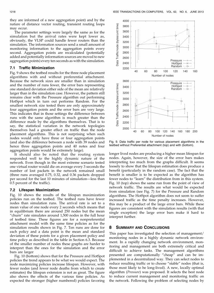
Fig. 9 shows the testbed results for the three node placementalgorithms with and without preferential attachment.Because the network sizes are smaller than in simulationand the number of runs fewer, the error bars representingone standard deviation either side of the mean are relativelylarger than in the simulation case. However, the pattern stillremains clear with the Pressure algorithm out performingHotSpot which in turn out performs Random. For thesmallest network size tested there are only approximatelyfour aggregation points and the error bars are very large.This indicates that in those settings the difference betweenruns with the same algorithm is much greater than thedifference made by the algorithms themselves. That is tosay, the statistical variation in the network topologiesthemselves had a greater effect on traffic than the nodeplacement algorithms. This is not surprising when suchnodes would only have three or four aggregation points(and also the difference between a node with 39 nodes andhence three aggregation points and 40 notes and fouraggregation points would be extremely large).

It should also be noted that the routing systemresponded well to the highly dynamic nature of thenetwork. Even though in the most extreme scenario testedone virtual router would die on average every 3 seconds thenumber of lost packets in the network remained small(three runs averaged 0.75, 0.32, and 0.36 packets droppedper second for the last 10 minutes of simulation—less than0.5 percent of the traffic).

7.2 Lifespan Maximization

Fig. 10 shows the results of the lifespan maximizationpolicies run on the testbed. The testbed runs have fewernodes than simulation runs. The arrival rate is set to amean value of one node every 2 seconds which means thatin equilibrium there are around 250 nodes but the mean“churn” rate simulates around 1,500 nodes in the full hourof testbed time. These figures are for a nonpreferentialattachment model with the same time policies as for thesimulation results shown in Fig. 7. Ten runs are done foreach policy and a data point is the mean and standarddeviation of these points for a given placement policy andtime policy as described in the table in Section 6.3. Becauseof the smaller number of nodes these graphs are harder tointerpret than the ones for the simulation and the errorbars are larger

Fig. 10 (bottom) shows that for the Pressure and HotSpotpolicies the trend appears to be what we would expect. Thenode maximizing policies increase lifespan. However, withfewer nodes (and fewer node deaths from which to createestimates) the lifespan extension is not as great. The figurealso shows the effects of the various time policies. Asexpected the stronger (higher numbered) policies favoring

longer lived nodes are producing a higher mean lifespan fornodes. Again, however, the size of the error bars makesinterpreting too much from the graphs difficult. It seemsloosely to show that the lifespan estimation does produce abenefit (particularly in the random case). The fact that thebenefit is smaller is to be expected as the algorithm hasfewer nodes to “learn” the distribution from in this system.Fig. 10 (top) shows the same run from the point of view ofnetwork traffic. The results are what would be expectedfrom simulation (see Fig. 7) for the Pressure and Randomalgorithms. The HotSpot algorithm does not seem to sufferincreased traffic as the time penalty increases. However,this may be a product of the large error bars. While thesefigures are consistent with the simulation results (with thatsingle exception) the large error bars make it hard tointerpret further.

8 SUMMARY AND CONCLUSIONS

This paper has investigated the selection of management/monitoring nodes in a highly dynamic network environ-ment. In a rapidly changing network environment, mon-itoring and management are both extremely critical anddifficult to achieve tasks. The management algorithmspresented are computationally “cheap” and can be im-plemented in a decentralized way. They can select nodes toreduce resulting traffic or to choose “stable” nodes (that is,those most likely to be long-lived). A new, locally optimalalgorithm (Pressure) was proposed. It selects the best nodeto reduce current management and monitoring traffic onthe network. Following the problem of selecting nodes by


Fig. 9. Data traffic per node for various placement algorithms in thetestbed without Preferential attachment (top) and with (bottom).

lifespan (that is the time remaining until the node exits thenetwork) is investigated. A simple estimator for remaininglifespan is given, together with an improved estimator withtail fitting. The combined algorithm that tackles nodeplacement and node-lifetime maximization is known asPressureTime.

The algorithms were tested both in simulation and on anew testbed environment, the VLSP testbed. The simulationenvironment tests networks with up to 5,000 nodes andwith a “churn” of 36,000 nodes (36,000 nodes in totalcreated of which approximately 5,000 are in use simulta-neously) over the simulation period. The testbed environ-ment used virtual routers running on JVM and emulatedaround 220 nodes with a “churn” of around 6,000 nodesover the simulation period.

The Pressure algorithm proved successful in reducing thetraffic generated by the monitoring nodes when comparedwith Random and HotSpot algorithms. In addition, thePressureTime algorithm combines node placement withlifespan maximization in a tunable way. To some extent,selecting optimally placed nodes and selecting nodes withthe longest lifespan are potentially “competing” problems(although in the case of the preferential attachment system itwas shown that sometimes long-lived nodes were also wellplaced). It was further demonstrated that the PressureTimealgorithm is tunable, so a system manager could optimizetheir system to choose management and monitoring nodeseither to reduce monitoring traffic, to increase monitoringnode lifespan, or some combination of these two goals.

Future work includes developing methods for control-ling virtual network stability. One problem is how to select

management nodes with regard to future placement of links

and nodes. Another problem is how to select links between

virtual nodes in order to maximize the stability of a

network, that is, the problem of choosing those virtual

links which reduce the risks of oscillations and disconnec-

tions within the network.

ACKNOWLEDGMENTS

This work is partially supported by the European Union

through the Autonomic Internet (AutoI) [3], [39], the

RESERVOIR project [12], and the UniverSELF [40] project

of the seventh Framework Program.

REFERENCES

[1] L. Mamatas, S. Clayman, M. Charalambides, A. Galis, and G.Pavlou, “Towards an Information Management Overlay forEmerging Networks,” Proc. IEEE/IFIP Network Operations andManagement Symp. (NOMS), 2010.

[2] S. Clayman, R.G. Clegg, L. Mamatas, G. Pavlou, and A. Galis,“Monitoring, Aggregation and Filtering for Efficient Managementof Virtual Networks,” Proc. Int’l Conf. Network and ServiceManagement (CNSM), Oct. 2011.

[3] A. Galis et al., Management Architecture and Systems for FutureInternet Networks. IOS Press, Apr. 2009.

[4] K. Akkaya, F. Senel, and B. McLaughlan, “Clustering of WirelessSensor and Actor Networks Based on Sensor Distribution andConnectivity,” J. Parallel Distributed Computig, vol. 69, pp. 573-587,June 2009.

[5] N.M.K. Chowdhury and R. Boutaba, “Network Virtualization:State of the Art and Research Challenges,” IEEE Comm. Magazine,vol. 47, no. 7, pp. 20-26, July 2009.

[6] M. Casado, T. Koponen, R. Ramanathan, and S. Shenker,“Virtualizing the Network Forwarding Plane,” Proc. CONEXTWorkshop Programmable Routers for Extensible Services of Tomorrow(PRESTO), 2010.

[7] T. Anderson, L. Peterson, S. Shenker, and J. Turner, “Overcomingthe Internet Impasse through Virtualization,” Computer, vol. 38,no. 4, pp. 34-41, Apr. 2005.

[8] N.M.K. Chowdhury and R. Boutaba, “A Survey of NetworkVirtualization,” Computer Networks, vol. 54, no. 5, pp. 862-876,2010.

[9] L. Andersson and T. Madsen, “Provider Provisioned VirtualPrivate Network (VPN) Terminology,” Internet Eng. Task Force,RFC 4026, Mar. 2005.

[10] A. Galis, S. Denazis, C. Brou, and C. Klein, Programmable Networksfor IP Service Deployment. Artech House Books, 2004.

[11] B. Rochwerger, D. Breitgand, D. Hadas, I. Llorente, R. Montero, P.Massonet, E. Levy, A. Galis, M. Villari, Y. Wolfsthal, E. Elmroth, J.Caceres, C. Vazquez, and J. Tordsson, “An Architecture forFederated Cloud Computing,” Cloud Computing, Springer, 2010.

[12] B. Rochwerger et al., “The RESERVOIR Model and Architecturefor Open Federated Cloud Computing,” IBM J. Research andDevelopment, vol. 53, no. 4, pp. 4:1-4:11, 2009.

[13] A. Malatras, G. Pavlou, and S. Sivavakeesar, “A ProgrammableFramework for the Deployment of Services and Protocols inMobile Ad Hoc Networks,” IEEE Trans. Network and ServiceManagement, vol. 4, no. 3, pp. 12-24, Dec. 2007.

[14] S.S. Yau, F. Karim, Y. Wang, B. Wang, and S.K.S. Gupta,“Reconfigurable Context-Sensitive Middleware for PervasiveComputing,” IEEE Pervasive Computing, vol. 1, no. 3, pp. 33-40,July-Sept. 2002.

[15] C. Olston, B.T. Loo, and J. Widom, “Adaptive Precision Setting forCached Approximate Values,” Proc. ACM SIGMOD Conf., pp. 355-366, 2001.

[16] G. Cormode, M. Garofalakis, S. Muthukrishnan, and R. Rastogi,“Holistic Aggregates in a Networked World: Distributed Trackingof Approximate Quantiles,” Proc. ACM SIGMOD Conf., pp. 25-36,2005.

[17] A. Sharaf, J. Beaver, A. Labrinidis, and K. Chrysanthis, “BalancingEnergy Efficiency and Quality of Aggregate Data in SensorNetworks,” The VLDB J., vol. 13, no. 4, pp. 384-403, 2004.


Fig. 10. Data traffic per node (top) and IAP lifespan (bottom) for one hour

on the testbed with various time policies.

[18] E. Welbourne, L. Battle, G. Cole, K. Gould, K. Rector, S. Raymer,M. Balazinska, and G. Borriello, “Building the Internet of ThingsUsing RFID: The RFID Ecosystem Experience,” IEEE InternetComputing, vol. 13, no. 3, pp. 48-55, May/June 2009.

[19] L. Atzori, A. Iera, and G. Morabito, “The Internet of Things: ASurvey,” Computer Networks, vol. 54, no. 15, pp. 2787-2805, 2010.

[20] A.G. Prieto and R. Stadler, “A-GAP: An Adaptive Protocol forContinuous Network Monitoring with Accuracy Objectives,” IEEETrans. Network and Service Management, vol. 4, no. 1, pp. 2-12, June2007.

[21] A.G. Prieto and R. Stadler, “Controlling Performance Trade-Offsin Adaptive Network Monitoring,” Proc. IFIP/IEEE 11th Int’l Symp.Integrated Network Management, 2009.

[22] A. Lahmadi, L. Andrey, and O. Festor, “Design and Validation ofan Analytical Model to Evaluate Monitoring Frameworks Limits,”Proc. Eighth Int’l Conf. Networks, 2009.

[23] C.H. Crawford and A. Dan, “eModel: Addressing the Need for aFlexible Modeling Framework in Autonomic Computing,” Proc.IEEE 10th Int’l Symp. Modeling, Analysis, and Simulation of ComputerSystems, 2002.

[24] X. Dong et al., “Autonomia: An Autonomic Computing Environ-ment,” Proc. IEEE Int’l Conf. Performance, Computing, and Comm.Conf., pp. 61-68, 2003.

[25] Y. Wang, E. Keller, B. Biskeborn, J. van der Merwe, and J. Rexford,“Virtual Routers on the Move: Live Router Migration as aNetwork-Management Primitive,” Proc. ACM SIGCOMM Conf.Data Comm., pp. 231-242, 2008.

[26] S. Clayman, A. Galis, and L. Mamatas, “Monitoring VirtualNetworks with Lattice,” Proc. IEEE/IFIP Int’l Workshop Manage-ment of Future Internet (ManFI ’10), 2010.

[27] C. Chaudet, E. Fleury, I.G. Lassous, H. Rivano, and M.-E. Voge,“Optimal Positioning of Active and Passive Monitoring Devices,”Proc. ACM Conf. Emerging Network Experiment and Technology(CoNEXT), pp. 71-82, 2005.

[28] K. Suh, Y. Guo, J. Kurose, and D. Towsley, “Locating NetworkMonitors: Complexity, Heuristics, and Coverage,” Proc. IEEEINFOCOM, vol. 1, pp. 351-361, 2005.

[29] C. Popi and O. Festor, “A Scheme for Dynamic Monitoring andLogging of Topology Information in Wireless Mesh Networks,”Proc. Network Operations and Management Symp., pp. 759 -762, 2008.

[30] U. Lee, B. Zhou, M. Gerla, E. Magistretti, P. Bellavista, and A.Corradi, “Mobeyes: Smart Mobs for Urban Monitoring with aVehicular Sensor Network,” Wireless Comm., vol. 13, no. 5, pp. 52-57, 2006.

[31] S. Hakimi, “Optimum Location of Switching Centers and theAbsolute Centers and Medians of a Graph,” Operations Research,vol. 12, pp. 450-459, 1964.

[32] Z. Drezner, “Dynamic Facility Location: The ProgressiveP-Median Problem,” Location Science, vol. 3, no. 1, pp. 1-7, 1995.

[33] E. Korach, S. Kutten, and S. Moran, “A Modular Technique for theDesign of Efficient Distributed Leader Finding Algorithms,” ACMTrans. Program. Language Systems, vol. 12, no. 1, pp. 84-101, 1990.

[34] L. DaSilva, “Pricing for QoS-Enabled Networks: A Survey,” IEEEComm. Surveys & Tutorials, vol. 3, no. 2, pp. 2-8, Second Quarter2000.

[35] M. Lindner, F.G. Marquez, C. Chapman, S. Clayman, and D.Hendriksson, “Cloud Supply Chain - A ComprehensiveFramework,” Proc. Second Int’l ICST Conf. Cloud Computing(CloudComp ’10), Oct. 2010.

[36] A.L. Barabasi and R. Albert, “Emergence of Scaling in RandomNetworks,” Science, vol. 286, no. 5439, pp. 509-512, 1999.

[37] R. Clegg, C.D. Cairano-Gilfedder, and S. Zhou, “A Critical Look atPower Law Modelling of the Internet,” Computer Comm., vol. 33,no. 3, pp. 259-268, 2010.

[38] C.D. Cairano-Gilfedder and R. Clegg, “A Decade of InternetResearch: Advances in Models and Practices,” BT Technology J.,vol. 23, no. 4, pp. 115-128, 2005.

[39] D. Macedo, Z. Movahedi, J. Rubio-Loyola, A. Astorga, G.Koumoutsos, and G. Pujolle, “The AutoI Approach for theOrchestration of Autonomic Networks,” Ann. Telecomm., vol. 66,pp. 243-255, 2011.

[40] UniverSELF Consortium, “UniverSELF Project,” http://www.univerself-project.eu/, 2012.

Richard G. Clegg received the PhD degree inmathematics and statistics from the University ofYork, in 2005. He is a senior research fellow atUniversity College London. His research inter-ests include network topologies, network trafficstatistics, and overlay network. He is a memberof the IEEE.

Stuart Clayman received the PhD degree incomputer science from University College Lon-don (UCL) in 1994. He has worked as a researchlecturer at Kingston University and is currently asenior research fellow at UCL. He coauthored30 conference and journal papers. His researchinterests and expertise lie in the areas ofsoftware engineering and programming para-digms, distributed systems, cloud systems,systems management, networked media, and

knowledge-based systems. He also has previous extensive experiencein the commercial arena undertaking architecture and development forsoftware engineering and networking systems.

George Pavlou received the chair of commu-nication networks at the Department of Electro-nic & Electrical Engineering, University CollegeLondon. Over the last 25 years, he has under-taken and directed research in networking andnetwork/service management, having exten-sively published in these areas. He has con-tributed to ISO, ITU-T, and IETF standardizationactivities and has been instrumental in anumber of key European and United Kingdom

projects that produced significant results. His current research interestsinclude traffic engineering, information-centric networking, autonomicnetworking, communications middleware, and infrastructure-less wire-less networks. He is a senior member of the IEEE.

Lefteris Mamatas is a postdoctoral researcherat the University College London. His researchinterests lie in the areas of autonomic networkand services management, delay-tolerant net-works, and energy efficient communication. Heparticipated in several international researchprojects, such as UniverSELF (FP7), AutonomicInternet (FP7), Ambient Networks (FP7), andExtending Internet into Space (European SpaceAgency). He published more than 30 papers in

international journals and conferences. He served as a TPC chair in theWWIC 2012 and E-DTN 2009 conferences. He is a member of the IEEE.

Alex Galis is a visiting professor at UniversityCollege London. He has coauthored sevenresearch books and more than 190 publicationsin journals and conferences in the Future Internetareas: networks, services, and management. Heacted as a PTC chair of 14 IEEE conferencesand reviewer in more than 100 IEEE conferenceshttp://www.ee.ucl.ac.uk/agalis. He worked as avice chairman for the ITU-T Focus Group onFuture Networks, which is defining design goals

and requirements in the Future Network http://www.itu.int/ITU-T/focusgroups/fn/index.html. He is a member of the IEEE.

. For more information on this or any other computing topic,please visit our Digital Library at www.computer.org/publications/dlib.


ieee transactions on computers, vol. 62, …gpavlou/publications/journal-papers/... · on the...

Documents