ieee transactions on image processing, vol. 14, no. 8...

IEEE TRANSACTIONS ON IMAGE PROCESSING, VOL. 14, NO. 8, AUGUST 2005 1125

Domain Decomposition for VariationalOptical-Flow Computation

Timo Kohlberger, Christoph Schnörr, Andrés Bruhn, and Joachim Weickert

Abstract—We present an approach to parallel variational op-tical-flow computation by using an arbitrary partition of the imageplane and iteratively solving related local variational problems as-sociated with each subdomain. The approach is particularly suitedfor implementations on PC clusters because interprocess commu-nication is minimized by restricting the exchange of data to a lowerdimensional interface. Our mathematical formulation supportsvarious generalizations to linear/nonlinear convex variationalapproaches, three-dimensional image sequences, spatiotemporalregularization, and unstructured geometries and triangulations.Results concerning the effects of interface preconditioning, as wellas runtime and communication volume measurements on a PCcluster, are presented. Our approach provides a major step towardreal-time two-dimensional image processing using off-the-shelfPC hardware and facilitates the efficient application of variationalapproaches to large-scale image processing problems.

Index Terms—Domain decomposition, image processing, opticalflow, parallel computation, partial differential equations, substruc-turing, variational techniques.

I. INTRODUCTION

TWO decades after the work of Horn and Schunck [19],both the mathematical understanding and algorithmic im-

plementations of variational approaches to optical-flow compu-tation have reached a stage where they outperform alternativeapproaches in many respects. Beginning with the work of Nagel[26], [27], more and more advanced versions of the prototypicalapproach of Horn and Schunck within the rich class of convexfunctionals have been developed including anisotropic and non-linear regularization preserving motion boundaries [36]. Con-cerning benchmark experiments [21], they compute accurateoptical flow everywhere in the image plane [36]. More robustlocal evaluation schemes, as well as spatiotemporal coherency,can be exploited within the same mathematical framework [4],[37].

A recurring argument against this class of approaches refersto the computational costs introduced by variational regulariza-tion. In our opinion, this argument is strongly misleading since

Manuscript received June 18, 2003; revised August 14, 2004. This workwas supported by the Deutsche Forschungsgemeinschaft (DFG) under GrantSchn457/4. The associate editor coordinating the review of this manuscript andapproving it for publication was Dr. Tamas Sziranyi.

T. Kohlberger and C. Schnörr are with the Computer Vision, Graphics,and Pattern Recognition Group, Department of Mathematics and ComputerScience, University of Mannheim, D-68131 Mannheim, Germany (e-mail:[email protected]; [email protected]).

A. Bruhn and J. Weickert are with the Mathematical Image Analysis Group,Department of Mathematics and Computer Science, Saarland University,D-66041 Saarbrücken, Germany (e-mail: [email protected]; [email protected]).

Digital Object Identifier 10.1109/TIP.2005.849778

it neglects the costs of alternative approaches related to heuristicpost processing of locally computed motion data (interpolationand segmentation). Moreover, besides computer vision, in manyfields of application, like medical imaging or remote sensing,variational regularization is the only mathematically sound wayfor taking into account prior knowledge about the structure ofmotion fields. This motivates our work on fast algorithms forvariational optical-flow computation.

In this context, the most common approach to acceleratecomputations is multigrid iteration [29], [38]. Again, beginningwith early work by Terzopoulos and Enkelmann, much progresshas been made during the last years [9], [13], [18], [20], [34],and current advanced implementations run in real-time for200 200 pixel sized image sequences on standard PC hard-ware [4]. Nevertheless, since the number of pixels per framesteadily increase in applications—e.g., 1500 700 pixels/framein fluid mechanics [22], and even more in three-dimensional(3-D) medical image sequences—parallelization of computa-tions is inevitable. Due to the nonlocal nature of variationalmodels, however, this is not a trivial task.

To illustrate the main difficulty of parallelizing variationaloptic flow approaches, Fig. 1(b) depicts the result of an ad hocparallelization where the variational problem was independentlysolved in each subregion. Due to the above-mentioned globalnature of variational motion estimation, strong artefacts ariseat the boundaries of the subregions. In contrast, our approachbelow solves the original variational problem by iteratively ex-changing data on the one-dimensional (1-D) boundaries of ad-jacent subregions.

A. Contribution and Organization

We present an approach to the parallelization of variationaloptical-flow computation which fulfills the following require-ments:

1) suitability for the implementation on PC clusters throughthe minimization of interprocess communication;

2) availability of a mathematical framework as basis for gen-eralizations to the whole class of linear and nonlinearvariational models characterized in [36].

Our approach draws upon the general mathematical literatureon domain decomposition, and especially upon substructuringmethods in connection with the solution of partial differentialequations [5], [30], [33]. After introducing some necessarymathematical prerequisites in Section II, we specifically derivein Section III an approach for computing the global variationalsolution in terms of an arbitrary number of local variationalsolutions, each of which can be computed in parallel on thepartitioned image domain (Fig. 2).

1057-7149/$20.00 © 2005 IEEE

1126 IEEE TRANSACTIONS ON IMAGE PROCESSING, VOL. 14, NO. 8, AUGUST 2005

Fig. 1. (a) True solution of an optic flow problem with global smoothness assumption. (b) Result of an ad hoc problem decomposition.

Fig. 2. Example of a squared 3� 3 partitioning of the image plane intosubdomains with shared boundaries � .

Concerning PC clusters as the target architecture for imple-mentations, an important feature of our approach is that in-terprocess communication is minimized by restricting the ex-change of data to a lower dimensional interface . This requiresa careful treatment of the variational models within each subdo-main (boundary conditions and discretization).

The results of Section III are then generalized to optical-flowcomputation by applying the common abstract variational for-mulation (see, e.g., [31]) in Section IV. Subsequently, a properdiscretization with finite elements is described.

Furthermore, this formulation ensures the applicability of ourapproach 1) to the whole class of quadratic variational models ascharacterized in [36] and 2) to nonquadratic discontinuity-pre-serving convex functionals [36] which can be minimized bymeans of suitable sequences of quadratic functional approxima-tions [35], [16].

In Section V, we report experimental results of a parallel im-plementation on a PC cluster for image sequences of (spatial)

sizes 512 512 and 2000 2000, and discuss the main charac-teristics of our approach: preconditioning the system of inter-face variables, including a coarse grid correction step, depen-dency of the convergence rate on the granularity of the domainpartition, and the scalability behavior for four to up to 144 pro-cessors. The results show that our approach provides a basisfor the computation of two-dimensional (2-D) optical flow inreal-time as well as for large-scale applications in other fields in-cluding 3-D medical imaging, remote sensing and experimentalfluid mechanics.

II. PRELIMINARIES AND MODEL PROBLEM

A. Mathematical Preliminaries and Notation

In this section, we introduce some notation and concepts nec-essary for the following. All details can be found in standardtextbooks like, e.g., [1] and [6].

Let denote opened and bounded domainswith “sufficiently smooth” (e.g., Lipschitz continuous) bound-aries and exterior unit normals .Furthermore, is a nonoverlapping partitionof the image plane , i.e., , , , andthe set of shared boundaries is defined by ,see Fig. 2 for an example.

We need the usual Sobolev space for second-order ellipticboundary value problems

The corresponding scalar product is defined as

KOHLBERGER et al.: DOMAIN DECOMPOSITION FOR VARIATIONAL OPTICAL-FLOW COMPUTATION 1127

with the scalar product of denoted with

We do not need the notion of “traces” and “trace spaces” in thefollowing. Hence, we loosely speak of functions with vanishingboundary values

Likewise, we use the symbolic notation

for the duality pairing with respect to the trace spaceand its dual, and call a function, as well.

Furthermore, we need any extensionof boundary values on to a function such that

.For and , the following version

of Green’s formula holds:

(1)

Throughout this paper, all functions are discretized with stan-dard conforming piecewise linear finite elements. To simplifynotation, we use the same symbols for some functionand the coefficient vector representing the approxima-tion of in the subspace spanned by the piecewise linearbasis functions

(2)

Furthermore, we use the same symbol for the vector obtainedby discretizing the action of some linear functional on somefunction . For example, we simply write and for thediscretized versions of the linear functionals and[with being a bilinear form and fixed].

Again, we refer to standard textbooks like, e.g., [6], [32], forthe discretization of boundary value problems with finite ele-ments.

B. Model Problem: The Definite Helmholtz Equation

For the reader’s convenience, we introduce in this section allrelevant concepts first for a model problem closely related to theprototypical variational problem (34) for optical-flow computa-tion. The generalization of the results in Section IV then will bestraightforward.

Let . We consider the following problem:

(3)

Vanishing of the first variation yields

with the bilinear form

Since

is strictly convex, and the global minimum is the unique so-lution to the variational equation:

(4)

By applying (1), partial integration yields the Euler–Lagrangeequation along with the natural boundary condition [14]

in on (5)

The solution to (4) is the so-called weak solution to (5).Discretization yields a linear system as the algebraic counter-

part of (4)

(6)

with a symmetric, sparse, and positive definite matrix .

C. Nonhomogeneous Boundary Conditions

The decomposition of problem (5) into a set of parallel solv-able problems (Section III) requires boundary conditions dif-ferent from the natural boundary condition in (5). We will col-lect necessary details in the following section.

1) Dirichlet Conditions: Suppose we wish to haveon , with some given function

in on on (7)

To obtain the corresponding variational formulation as basis ofa proper finite element discretization, we define the subspace

The variational formulation of (7) then reads: Findsuch that

(8)

The desired solution is , with an arbitraryextension .

2) Neumann Conditions: Alternatively, suppose we wish tohave on , with a given function

in on on(9)


The corresponding variational formulation reads: Findsuch that

(10)

III. PROBLEM DECOMPOSITION AND PARALLELIZATION

A. Two Domains

1) Approach: Let be a partition of with a commonboundary , as detailed in Section II-A. Wedenote the corresponding function spaces with , . In thefollowing, superscripts refer to subdomains.

We wish to represent from (5) by two functions ,which are computed by solving two related problems

in , , respectively. The relation

(11)

obviously holds if the following is true:

in on (12)

in on (13)

on (14)

on (15)

We observe that (5) cannot simply be solved by separatelycomputing and in each domain , because the naturalboundary conditions have to be changed on , due to (14) and(15).

As a consequence, in order to solve the system of (12)–(15),we equate the restriction to the interface of the two solutions

, to (12) and (13), due to (14), , andsubstitute into (15). This will be achieved by means of theSteklov–Poincaré operator introduced in the following. Oncethe resulting equation has been solved for , the functionsand then follow from the substitution of back into (12)and (13) with boundary condition (14). This approach is knownas substructuring, cf., e.g., [33].

2) Steklov–Poincaré Operator : In the previous section,we have shown that in order to solve system (12)–(15), we haveto make explicit the dependency between and of thesolution to a boundary value problem.

Let be the solution to problem (7). We decompose intotwo functions

which are the unique solutions to the following problems:

in on on (16)

in on on (17)

Clearly, we have and

(18)

(19)

The definition of the Steklov–Poincaré operator is (cf. e.g.,[30])

(20)

Applying this mapping to the solutions , of (12) and (13)in the domains and , respectively, (15) becomes

(21)

with due to (14). Equation (21) is denotedas the interface equation. It remains to solve this equation for

. Since is known to be a symmetric, and positive definiteoperator, preconditioned conjugate gradient (PCG) methods canbe applied for solving (21), which will be detailed later on. Tothis end, we have to make explicit how the action of and ,respectively, can be computed. In the following two sections weshow that this amounts to solving two associated boundary valueproblems.

3) Action of : By (8), the variational formulation ofproblem (16) reads

(22)

Discretization yields a linear system for (cf. the conventionstated after (1) regarding notation)

(23)

where index refers to all nodal variables excluding those on. The extension operator supplements the boundary values

with zeros as values of interior nodal variables, and, thus,defines, by using (2), a function .

Let us compare the systems (23) and (6), the latter corre-sponding to the boundary value problem (5). To this end, wedecompose the linear system (6) according to

Note that the dimension of this linear system is larger becauseruns through in (4), whereas in (22), only varies in .Now, consider , with from (22) and

(23), respectively, and let vary in . Note that for, ,

due to (22). For and taking into considerationfrom (16), we obtain by (1)

(24)

Since due to (16), discretization of this variationalequation yields the linear system

(25)

from which we conclude by algebraically eliminating [cf.definition (20)]

(26)


which is also known as the Schur complement of . Hence, theaction of on some boundary data involves the solution ofproblems (22) and (23).

4) Action of : In order to make the action of ex-plicit, as well, we may formally invert (26). Since is dense, thisis not advisable, however. Therefore, in practice, one solves theNeumann problem (24) for with and given boundarydata (compare with (10)) and obtains by restriction to theinterface . Alternatively, this can also be alge-braically derived from (25) by the following factorization:

Inverting this matrix yields

Hence

(27)

5) Interface Equation: Using the results of the previous sec-tions, we return now to (21) in connection with solving thesystem of (12)–(15).

Suppose the boundary values on theinterface separating and were known. Then, and

within and , respectively, can be exactly computed asdiscussed for problem (7). Here, is given by

Thus, it remains to compute the unknown boundary function. This will be done by solving (15) using the

formulation (21).To set up (21), we have to compute , , 2. This can

be reached by the same procedure used to compute (24). Since, , 2, we obtain

Discretization yields the linear systems

(28)Due to the system (12)–(15), we have to solve these two linearsystems simultaneously, along with the system (25) applied toeither domain , , 2. Since , summationof the two systems (25) and (28) for each domain, respectively,gives

We combine these equations into a single system

(29)

where

By solving the first two equations for , and substitutioninto the third equation of (29), we conclude that (15) holds if

By applying (26), we finally obtain

(30)

which is also known as the Schur complement problem of (6).Recall that (30) was derived by substituting (12)–(14) into (15).Accordingly, imposing the solution to (30) as boundary con-ditions as required in (14), the functions and can be com-puted from (12) and (13) such that (11) holds! In addition, thecomputation of , needed duringCG iteration, can be carried out in parallel.

B. Multiple Domains

In this section, we generalize the results to the case of multiplesubdomains (see Fig. 2). Furthermore, we discusspreconditioners for the interface equation, a critical issue for anefficient parallel implementation of the overall approach.

1) Interface Equation: Let denote the restriction of thevector of nodal variables on the interface to those on

. Analogously to the case of two domains detailed above, theinterface equation for multiple domains reads

(31)

Once the values on in the interface are known, the inner nodalvariables can be determined by

(32)

2) Interface Preconditioners: While a fine partition ofinto a large number of subdomains leads to small-sized and“computationally cheap” local problems in each subdomain, thecondition number of the Steklov–Poincaré operator more andmore deteriorates [30]. As a consequence, preconditioning ofthe interface equation becomes crucial for an efficient parallelimplementation.

Among different but provably optimal (“spectrally equiva-lent”) families of preconditioners (cf. [5], [33]), we examinedthe Neumann–Neumann preconditioner (NN) [2], [7], [23] and


the balancing-Neumann–Neumann preconditioner (BNN) [8],[24], [25]. These preconditioners applied in connection withconjugate gradient iteration [15] preserve the symmetry ofand have natural extensions to more general problems relatedto 3-D image sequences or unstructured geometries and/ortriangulations.

The NN preconditioner reads

(33)

where denotes a diagonal scaling matrix whose entriesare the reciprocals of the number of subdomains shared by nodes

on . Note that the computation of leads to a localproblem in subdomain [see Section III-A, 4)] which can besolved in parallel for all subdomains.

The BNN preconditioner reads

In comparison with (33), this preconditioner additionally car-ries out a correction step (denoted as “balancing” in literature)before and after the application of the NN preconditioner on acoarse grid given by the partition of the domain into subdo-mains (see Fig. 2).

The restriction operator sums up the weighted values onthe boundary of each subdomain, where the weights are givenby the inverse of the number of subdomains sharing a particularnode, i.e.

if node is on an edge ofif node is on a vertex ofelse.

Then, is defined by .Note that is a dense matrix of small dimension (related to

the number of subdomains) which can be efficiently inverted bya standard direct method.

IV. VARIATIONAL OPTICAL FLOW COMPUTATION

We generalize the results obtained so far to optical-flow com-putation. To this end, we replace model problem (3) by the vari-ational approach (34). As explained in Section I, this approachrepresents a large class of alternative approaches to which ourdecomposition approach can be applied.

A. Variational Problem

In order to point out the common problem structure with themodel problem discussed in Section II-B, we denote in this sec-tion the image function with , and keep the symbol for thelinear functional induced by the image data which in connectionwith optical-flow computation differs from in Section II-B[see (37)].

Throughout this section, denotes the gra-dient with respect to spatial variables, the partial derivativewith respect to time, and , denotevector fields in the linear space [see [31]].

With this notational convention, the variational problem to besolved reads [19]

(34)Analogously to the derivation in Section II-B, vanishing of

the first variation of the functional in (34) yields the varia-tional equation

(35)

where

(36)

(37)

Under weak conditions with respect to the image data , theexistence of a constant was proven in [31] such that

As a consequence, in (34) is strictly convex and its globalminimum is the unique solution to the variational (35). Par-tially integrating in (35) by means of (1), we derive the systemof Euler–Lagrange equations

in on (38)

where

We emphasize that the prototypical problem (34) can beeasily generalized to other convex functionals as characterizedin [36]. In the experiments presented in the following, we haveutilized the CLG approach [4], which replaces the first termin (34) by the spatiotemporal structure tensor [28], [37], withsmoothness parameter . Modifying (36) and (37) accord-ingly, their discrete representations (39) can be automaticallycomputed by discretization with finite elements, and our de-composition approach for parallelization can be immediatelyapplied.

B. Discretization

To approximate the vector field numerically, (35) is dis-cretized by piecewise linear finite elements over the triangu-lated section of the image plane. We arrange the vectors ofnodal variables , corresponding to the finite element dis-cretizations of , as follows: (cf.Section II-A). Taking into consideration the symmetry of thebilinear form (36), this induces the following block structure ofthe discretized version of (35)

(39)


where ,

Here, denotes the linear basis function corresponding tothe nodal variable or , respectively. Apart from theblock structure of this linear system , all results ofSections III-A and III-B carry over verbatim.

V. PARALLEL IMPLEMENTATION AND EXPERIMENTS

A. Parallel Implementation

As already mentioned, the great advantage of domain decom-position methods, and especially of substructuring methods inour case, is their inherent coarse-grain parallelism. In partic-ular, since the Steklov–Poincaré operator can be written as

, its application in a PCG iteration for solving(30) or (31), respectively, can be seperated into simultaneousapplications of the local operators on . This mainlyamounts to solving local Dirichlet systems as detailed in Sec-tion III-A, 3). Analogously, the computation of preconditioner

can be parallelized in solving the local Neumann problemsassociated with each occurence of , as described in Sec-tion III-A, 4), in parallel.

In a parallel framework, those local problems are usuallysolved in slave processes which exchange their local data witha dedicated master process carrying out the PCG iteration. Insuch a setting, the restriction operators , as introduced in Sec-tion III-B 1), correspond to a scatter operation, and it transposes

to a reduce operation between the master process andthe slave processes. In particular, a scatter operation consists ofsending to each slave process, associated with subdomain ,the subset of nodal variables. Conversely, the transposedoperator amounts to a reduce operation, i.e., receivingand adding the nodal values of all local shared boundaries.

Additionally, the coarse operator has tobe inverted in connection with the BNN preconditioner .Since is global, as is , parallelization is not applicable here.Therefore, is computed explicitly during initialization. Then,the associated system is solved serially during PCGiteration. Since is much smaller than , the nonparallel com-putational effort for doing so is negligible.

It remains to find an efficient scheme for calculating the en-tries of . We use a column-wise initialization by

th unit vector

which has the inherent disadvantage of the number of appli-cations being equal the number of subdomains. Taking a closer

Fig. 3. Initialization scheme for the coarse grid operator S on 10� 10subdomains. Each gray cross at a particular depicts the area of nodes whereR S(R ) e is nonzero.

TABLE ICG VERSUS PCG ITERATION OF THE INTERFACE PROBLEM

look at shows that its th column affects only the sharedboundaries of the subdomain , as well as its left, right, upper,and lower neighboring subdomains, if any, as well as the nodalvariables at the vertices of the diagonal neighbors. Since thelatter ones have turned out to be negligible in practice, the initial-ization of can be partially parallelized by computing everyfourth column of in a group of columns corresponding toevery second row of the subdomain partition; see Fig. 3 for il-lustration. With this optimized initialization scheme, the numberof initial applications of is always eight, independent of thetotal number of subdomains.

It remains the calculation of the right-hand sides of (30) or(31), respectively, as well as the final calculation of the innernodal variables by (12)–(15) or (32). Both provide inherent par-allelism by solving the corresponding Dirichlet system simulta-neously on every subdomain.

B. Experimental Setting and Input Data

We conducted different experiments in order to investigatethe following aspects of the described domain decompositionmethod:

1) effect of interface preconditioning on the convergencerate;

2) comparison of the convergence rates utilizing the NNor BNN preconditioner for different numbers of subdo-mains;

3) the total runtime and the interprocess communicationvolume depending on the number of subdomains foreach preconditioner in comparison to fast nonparallelmultigrid solving.

For ease of implementation, the image plane was parti-tioned into equally sized, quadratic subdomains in all ex-periments. The parameter values of the CLG motion estimationwere , , and , while the intensity


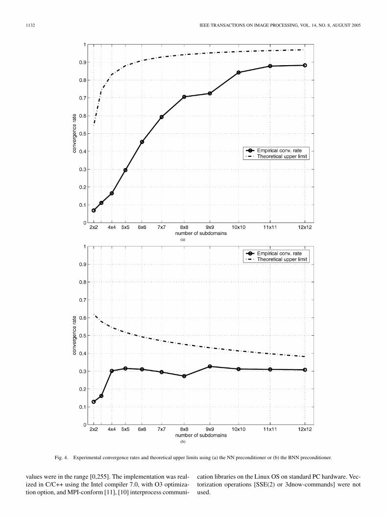
Fig. 4. Experimental convergence rates and theoretical upper limits using (a) the NN preconditioner or (b) the BNN preconditioner.

values were in the range [0,255]. The implementation was real-ized in C/C++ using the Intel compiler 7.0, with O3 optimiza-tion option, and MPI-conform [11], [10] interprocess communi-

cation libraries on the Linux OS on standard PC hardware. Vec-torization operations [SSE(2) or 3dnow-commands] were notused.


Fig. 5. Number of iterations for an error threshold of 10 using NN or BNN preconditioning on frame 16 and 17 of the marble sequence (512� 512).

C. Effect of Interface Preconditioning

In order to investigate the influence of an interface precon-ditioner in general, (31) was solved for without precondi-tioning and also by applying the NN preconditioner. As inputimages frame 16 and 17 of the marble sequence.1 As a localsolver, PCG iteration was also used, iterating until the relativeresidual error was below . Table I depicts the number ofnecessary outer (P)CG iterations to reach an residual error of

, i.e., , with denoting ther.h.s. of (31). It clearly shows that, in agreement with theory[30], the system becomes more and more ill conditioned if thenumber of subdomains increases. Using the NN preconditioner(33), however, largely compensates this effect and enablesshorter computation times through parallelization.

D. Convergence Rate Studies

In this experiment, we compared the linear convergence ratebased on the original problem (38) using NN or BNN precon-

ditioning for varying numbers of subdomains . PCG iterationwas also used as local solver here. The convergence rates wheredetermined by , withbeing the error after iterations and . The examinedrates are depicted in Fig. 4 for each preconditioner (solid lines).They clearly show that the convergence rate using the nonbal-ancing preconditioner grows with the number of subdomainswhereas they remain nearly constant for the preconditioner in-volving a coarse grid correction step.

1Created in 1993 by Michael Otte, Institut für Algorithmen und KognitiveSysteme, University of Karlsruhe, Germany, available at http://i21www.ira.uka.de/image_sequences.

Furthermore, these results are consistent with theoreticalupper limits which can be derived from approximations of thecondition numbers of the preconditioned operatorsand , namely [7], [23] , [25]

(40)

and

(41)

with denoting the mesh sizes of the coarse grid, which cor-responds to the subdomain partition, and denoting the finediscretization grid, as well as some constants , . It iswell known, cf. e.g., [15, p. 272], that the convergence rate ofPCG iteration depends on the condition number by

with (42)

The observations are in agreement with the theory and espe-cially the presence of the term in the bound of the NN pre-conditioner, leading to a worse convergence for an increasingnumber of subdomains (which is of order ) whereaswith the two-level preconditioner it remains nearly constant dueto the influence of the coarse grid couplings.

In a further experiment, we compared the number of iterationsnecessary for the residual error to fall below using

the NN and BNN preconditioner. Results are shown in Fig. 5.Thus, the BNN preconditioner is much closer to an optimal pre-conditioner making the convergence rate independent w.r.t. both


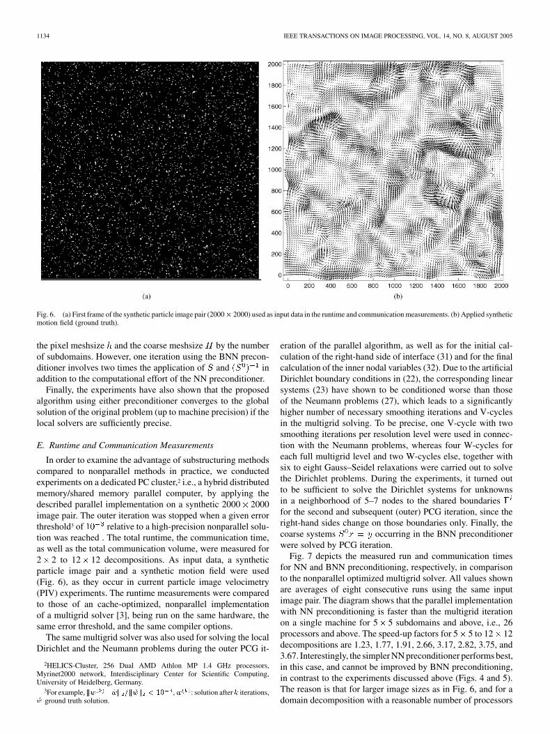
Fig. 6. (a) First frame of the synthetic particle image pair (2000� 2000) used as input data in the runtime and communication measurements. (b) Applied syntheticmotion field (ground truth).

the pixel meshsize and the coarse meshsize by the numberof subdomains. However, one iteration using the BNN precon-ditioner involves two times the application of and inaddition to the computational effort of the NN preconditioner.

Finally, the experiments have also shown that the proposedalgorithm using either preconditioner converges to the globalsolution of the original problem (up to machine precision) if thelocal solvers are sufficiently precise.

E. Runtime and Communication Measurements

In order to examine the advantage of substructuring methodscompared to nonparallel methods in practice, we conductedexperiments on a dedicated PC cluster,2 i.e., a hybrid distributedmemory/shared memory parallel computer, by applying thedescribed parallel implementation on a synthetic 2000 2000image pair. The outer iteration was stopped when a given errorthreshold3 of relative to a high-precision nonparallel solu-tion was reached . The total runtime, the communication time,as well as the total communication volume, were measured for2 2 to 12 12 decompositions. As input data, a syntheticparticle image pair and a synthetic motion field were used(Fig. 6), as they occur in current particle image velocimetry(PIV) experiments. The runtime measurements were comparedto those of an cache-optimized, nonparallel implementationof a multigrid solver [3], being run on the same hardware, thesame error threshold, and the same compiler options.

The same multigrid solver was also used for solving the localDirichlet and the Neumann problems during the outer PCG it-

2HELICS-Cluster, 256 Dual AMD Athlon MP 1.4 GHz processors,Myrinet2000 network, Interdisciplinary Center for Scientific Computing,University of Heidelberg, Germany.

3For example, kw �wk =kwk < 10 ,w : solution after k iterations,w ground truth solution.

eration of the parallel algorithm, as well as for the initial cal-culation of the right-hand side of interface (31) and for the finalcalculation of the inner nodal variables (32). Due to the artificialDirichlet boundary conditions in (22), the corresponding linearsystems (23) have shown to be conditioned worse than thoseof the Neumann problems (27), which leads to a significantlyhigher number of necessary smoothing iterations and V-cyclesin the multigrid solving. To be precise, one V-cycle with twosmoothing iterations per resolution level were used in connec-tion with the Neumann problems, whereas four W-cycles foreach full multigrid level and two W-cycles else, together withsix to eight Gauss–Seidel relaxations were carried out to solvethe Dirichlet problems. During the experiments, it turned outto be sufficient to solve the Dirichlet systems for unknownsin a neighborhood of 5–7 nodes to the shared boundariesfor the second and subsequent (outer) PCG iteration, since theright-hand sides change on those boundaries only. Finally, thecoarse systems occurring in the BNN preconditionerwere solved by PCG iteration.

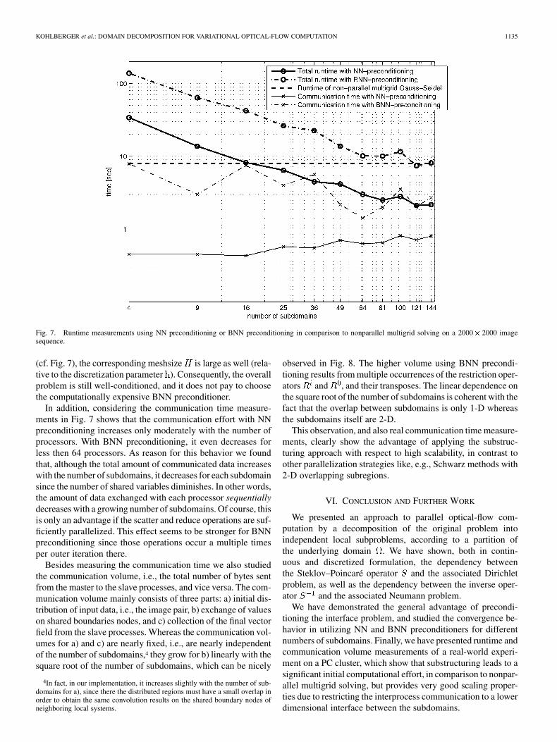
Fig. 7 depicts the measured run and communication timesfor NN and BNN preconditioning, respectively, in comparisonto the nonparallel optimized multigrid solver. All values shownare averages of eight consecutive runs using the same inputimage pair. The diagram shows that the parallel implementationwith NN preconditioning is faster than the multigrid iterationon a single machine for 5 5 subdomains and above, i.e., 26processors and above. The speed-up factors for 5 5 to 12 12decompositions are 1.23, 1.77, 1.91, 2.66, 3.17, 2.82, 3.75, and3.67. Interestingly, the simpler NN preconditioner performs best,in this case, and cannot be improved by BNN preconditioning,in contrast to the experiments discussed above (Figs. 4 and 5).The reason is that for larger image sizes as in Fig. 6, and for adomain decomposition with a reasonable number of processors


Fig. 7. Runtime measurements using NN preconditioning or BNN preconditioning in comparison to nonparallel multigrid solving on a 2000� 2000 imagesequence.

(cf. Fig. 7), the corresponding meshsize is large as well (rela-tive to the discretization parameter ). Consequently, the overallproblem is still well-conditioned, and it does not pay to choosethe computationally expensive BNN preconditioner.

In addition, considering the communication time measure-ments in Fig. 7 shows that the communication effort with NNpreconditioning increases only moderately with the number ofprocessors. With BNN preconditioning, it even decreases forless then 64 processors. As reason for this behavior we foundthat, although the total amount of communicated data increaseswith the number of subdomains, it decreases for each subdomainsince the number of shared variables diminishes. In other words,the amount of data exchanged with each processor sequentiallydecreases with a growing number of subdomains. Of course, thisis only an advantage if the scatter and reduce operations are suf-ficiently parallelized. This effect seems to be stronger for BNNpreconditioning since those operations occur a multiple timesper outer iteration there.

Besides measuring the communication time we also studiedthe communication volume, i.e., the total number of bytes sentfrom the master to the slave processes, and vice versa. The com-munication volume mainly consists of three parts: a) initial dis-tribution of input data, i.e., the image pair, b) exchange of valueson shared boundaries nodes, and c) collection of the final vectorfield from the slave processes. Whereas the communication vol-umes for a) and c) are nearly fixed, i.e., are nearly independentof the number of subdomains,4 they grow for b) linearly with thesquare root of the number of subdomains, which can be nicely

4In fact, in our implementation, it increases slightly with the number of sub-domains for a), since there the distributed regions must have a small overlap inorder to obtain the same convolution results on the shared boundary nodes ofneighboring local systems.

observed in Fig. 8. The higher volume using BNN precondi-tioning results from multiple occurrences of the restriction oper-ators and , and their transposes. The linear dependence onthe square root of the number of subdomains is coherent with thefact that the overlap between subdomains is only 1-D whereasthe subdomains itself are 2-D.

This observation, and also real communication time measure-ments, clearly show the advantage of applying the substruc-turing approach with respect to high scalability, in contrast toother parallelization strategies like, e.g., Schwarz methods with2-D overlapping subregions.

VI. CONCLUSION AND FURTHER WORK

We presented an approach to parallel optical-flow com-putation by a decomposition of the original problem intoindependent local subproblems, according to a partition ofthe underlying domain . We have shown, both in contin-uous and discretized formulation, the dependency betweenthe Steklov–Poincaré operator and the associated Dirichletproblem, as well as the dependency between the inverse oper-ator and the associated Neumann problem.

We have demonstrated the general advantage of precondi-tioning the interface problem, and studied the convergence be-havior in utilizing NN and BNN preconditioners for differentnumbers of subdomains. Finally, we have presented runtime andcommunication volume measurements of a real-world experi-ment on a PC cluster, which show that substructuring leads to asignificant initial computational effort, in comparison to nonpar-allel multigrid solving, but provides very good scaling proper-ties due to restricting the interprocess communication to a lowerdimensional interface between the subdomains.


Fig. 8. Measured communication volume (between master and slave processes) using NN or BNN preconditioning.

Due to the components chosen for our approach and the use ofconforming finite element discretization, our approach is appli-cable, in principle, to the whole class of quadratic variational ap-proaches for optical-flow computation and less-structured prob-lems involving irregularly shaped domains and nonuniform tri-angulations (i.e., experimental fluid dynamics).

By applying our approach to a higher number of processorsand by exploiting vectorization and local parallelization in eachprocessing node, real-time 2-D optic-flow estimation on largeimage sequences will come into reach on standard PC hardware.Furthermore, we will extend our work to nonquadratic varia-tional approaches, like total variation-based regularization, forexample, where sequences of quadratic variational approxima-tions are used to compute minimizers.

Finally, it might be worthwile to use multigrid iteration notonly as subdomain solver, but to consider parallelization atcoarse grid levels [12], [17].

REFERENCES

[1] J. P. Aubin, Approximation of Elliptic Boundary-Value Problem. NewYork: Wiley, 1972.

[2] J.-F. Bourgat, R. Glowinski, P. Le Tallec, and M. Vidrascu, “Variationalformulation and algorithm for trace operator in domain decomposi-tion calculations,” in Domain Decomposition Methods, T. Chan, R.Glowinski, J. Périaux, and O. Widlund, Eds. Philadelphia, PA: SIAM,1989, pp. 3–16.

[3] A. Bruhn, J. Weickert, C. Feddern, T. Kohlberger, and C. Schnörr,“Variational optical flow computation in real-time,” IEEE Trans. ImageProcess., to be published.

[4] A. Bruhn, J. Weickert, and C. Schnörr, “Lucas/Kanade meetsHorn/Schunck: Combining local and global optic flow methods,”Int. J. Comput. Vis., to be published.

[5] T. F. Chan and T. P. Mathew, “Domain decomposition algorithms,” inActa Numerica 1994. Cambridge, U.K.: Cambridge Univ. Press, 1994,pp. 61–143.

[6] P. G. Ciarlet, The Finite Element Method for Elliptic Problem. Ams-terdam, The Netherlands: North-Holland, 1978.

[7] Y.-H. De Roeck and P. Le Tallec, “Analysis and test of a local domaindecomposition preconditioner,” in Proc. 4th Int. Symp. Domain Decom-position Methods for Part. Diff. Equations, R. Glowinsiki, Y. Kuznetsov,G. Meurant, J Périaux, and O. Widlund, Eds., Philadelphia, PA, 1991, pp.112–128.

[8] M. Dryja and O. B. Widlund, “Schwarz methods of Neumann-Neumanntype for three-dimensional elliptic finite element problems,” Commun.Pure Appl. Math., vol. 48, pp. 121–155, 1995.

[9] W. Enkelmann, “Investigation of multigrid algorithms for the estimationof optical flow fields in image sequences,” Comput. Vis. Graph. Imag.Process., vol. 43, pp. 150–177, 1987.

[10] “Message passing interface forum,” in MPI-2: Extensions to the Mes-sage-Passing Interface Univ. Tennessee, Knoxville, 1995.

[11] “Message passing interface forum,” in MPI: A Message-Passing Inter-face Standard Univ. Tennessee, Knoxville, 1995.

[12] U. Gärtel and K. Ressel, “Parallel multigrid: Grid partitioning versusdomain decomposition,” in Proc. 10th Int. Conf. Computing Methods inApplied Sciences and Engineering, R. Glowinski, Ed., New York, 1992,pp. 559–568.

[13] S. Ghosal and P. Vanek, “A fast scalable algorithm for discontinuousoptical flow estimation,” IEEE Trans. Pattern Anal. Mach. Intell., vol.18, no. 2, pp. 181–194, Feb. 1996.

[14] W. Hackbusch, Theorie und Numerik Elliptischer Differentialgle-ichungen. Stuttgart, Germany: B. G. Teubner, 1986.

[15] , Iterative Solution of Large Sparse Systems of Equations. Berlin,Germany: Springer, 1993.

[16] J. Heers, C. Schnörr, and H. S. Stiehl, “Globally–convergent iterativenumerical schemes for non–linear variational image smoothing and seg-mentation on a multi–processor machine,” IEEE Trans. Image Process.,vol. 10, no. 6, pp. 852–864, Jun. 2001.

[17] B. Heise and M. Jung, “Comparison of parallel solvers for nonlinear el-liptic problems based on domain decomposition ideas,” Johannes KeplerUniv. Linz, Inst. Math., Linz, Austria, Tech. Rep. 494, 1995.

[18] F. Heitz, P. Perez, and P. Bouthemy, “Multiscale minimization of globalenergy functions in some visual recovery problems,” CVGIP: Image Un-derstanding, vol. 59, no. 1, pp. 125–134, 1994.

[19] B. K. P. Horn and B. G. Schunck, “Determining optical flow,” Artif. In-tell., vol. 17, pp. 185–203, 1981.

[20] S. H. Hwang and S. U. Lee, “A hierarchical optical flow estimation al-gorithm based on the interlevel motion smoothness constraint,” PatternRecognit., vol. 26, no. 6, pp. 939–952, 1993.


[21] D. J. Fleet, J. L. Barron, and S. S. Beauchemin, “Perfomance of opticalflow techniques,” Int. J. Comput. Vis., vol. 1, no. 12, pp. 43–77, Feb.1994.

[22] T. Kohlberger, E. Mémin, and C. Schnörr, “Variational dense motionestimation using the helmholtz decomposition,” in Proc. 4th Int. Conf.Scale-Space Theories in Computer Vision, ScaleSpace, vol. 2695,LNCS, L. D. Griffin and M. Lillholm, Eds., 2003, pp. 432–448.

[23] P. Le Tallec, Y.-H. De Roeck, and M. Vidrascu, “Domain decomposi-tion methods for large linearly elliptic three dimensional problems,” J.Comput. Appl. Math., vol. 34, pp. 93–117, 1991.

[24] J. Mandel, “Balancing domain decomposition,” Commun. Numer. Math.Eng., vol. 9, pp. 233–241, 1993.

[25] J. Mandel and M. Brezina, “Balancing domain decomposition: Theoryand performance in two and three dimensions,” Comput. Math. Group,Univ. Colorado, Denver, Tech. Rep., vol. 1, 1993.

[26] H. H. Nagel, “Constraints for the estimation of displacement vectorfields from image sequences,” in Proc. 8th Int. J. Conf. Artif. Intell.,Karlsruhe, Germany, 1983, pp. 945–951.

[27] , “On the estimation of optical flow: Relations between differentapproaches and some new results,” Artif. Intell., vol. 33, pp. 299–324,1987.

[28] , “Extending the ’oriented smoothness constraint’ into the temporaldomain an the estimation of derivatives of optical flow,” in Proc. Com-puter Vision ECCV, vol. 427, O. Faugeras, Ed., Berlin, Germany, 1990,pp. 139–148.

[29] P. Oswald, Multilevel Finite Element Approximation. Stuttgart, Ger-many: B. G. Teubner, 1994.

[30] A. Quarteroni and A. Valli, Domain Decomposition Methods for PartialDifferential Equations. Oxford, U.K.: Oxford Univ. Press, 1999.

[31] C. Schnörr, “Determining optical flow for irregular domains by mini-mizing quadratic functionals of a certain class,” Int. J. Comput. Vis., vol.6, no. 1, pp. 25–38, 1991.

[32] H. R. Schwarz, Methode der Finiten Elemente. Stuttgart, Germany: B.G. Teubner, 1980.

[33] B. Smith, P. Bjørstad, and W. Gropp, Domain Decomposition: ParallelMultilevel Methods for the Solution of Elliptic Partial Differential Equa-tions. Cambridge, U.K.: Cambridge Univ. Press, 1996.

[34] D. Terzopoulos, “Multilevel computational processes for visual surfacereconstruction,” Comput. Vis., Graph., Image Process., vol. 24, pp.52–96, 1983.

[35] R. V. Vogel and M. E. Oman, “Iterative methods for total variation de-noising,” SIAM J. Sci. Comput., vol. 17, no. 1, pp. 227–238, 1996.

[36] J. Weickert and C. Schnörr, “A theoretical framework for convex reg-ularizers in PDE–based computation of image motion,” Int. J. Comput.Vis., vol. 45, no. 3, pp. 245–264, 2001.

[37] , “Variational optic flow computation with a spatio-temporalsmoothness constraint,” J. Math. Imag. Vis., vol. 14, no. 3, pp. 245–255,2001.

[38] P. Wesseling, An Introduction to Multigrid Methods. New York: Wiley,1992.

Timo Kohlberger studied computer engineering atthe University of Mannheim, Mannheim, Germany,where, during his studies, he was supported by theGerman National Merit Foundation, and from whichhe received the Diplom (Master) degree in computerscience in 2001, and where he is currently pursuingthe Ph.D. degree.

Since October 2001, he has been with the CVGPRGroup of the University of Mannheim. His presentresearch interests include parallelization techniquesapplied to image motion computation and computer

vision, the design of novel approaches in motion estimation, as well as trackingand suveillance systems.

Christoph Schnörr received the Dipl.–Ing. degreein electrical engineering and the Dr.rer.nat. degree incomputer science from the Technical University ofKarlsruhe, Karlsruhe, Germany, and the Habilitationdegree in computer science from the University ofHamburg, Hamburg, Germany, in 1987, 1991, and1998, respectively.

He held the position of Researcher at the Fraun-hofer Institute for Information and Data Processing(IITB), Karlsruhe, from 1987 to 1992 and Researcherand Assistant Professor within the Cognitive Systems

Group, University of Hamburg. During 1996, he was a Visiting Researcher at theComputer Vision and Active Perception Laboratory, KTH, Stockholm, Sweden.Since 1999, he has been with the Department of Mathematics and ComputerScience, University of Mannheim, Mannheim, Germany, where he set up andis the Head of the Computer Vision, Graphics, and Pattern Recognition Group.He serves on the editorial board of the Journal of Mathematical Imaging andVision. His research interests include computer vision, pattern recognition, andrelated aspects of mathematical modeling and optimization.

Dr. Schnörr is a member of DAGM, SIAM, and SIAGIS. He is Co-Editor-in-Chief of the International Journal of Computer Vision and he serves on theeditorial board of the Journal of Mathematical Imaging and Vision.

Andrés Bruhn received the M.Sc. degree in com-puter engineering from the University of Mannheim,Mannheim, Germany, in 2001. He is currently pur-suing the Ph.D. degree in computer science at Saar-land University, Saarbrücken, Germany.

He was a Research Assistant at the University ofMannheim from October to November 2001. SinceDecember 2001, he has been with the MathematicalImage Analysis Group, Department of Mathematicsand Computer Science, Saarland University. Hiscurrent research interests include optical-flow esti-

mation, diffusion filtering, and fast numerical schemes for image processingand computer vision.

Mr. Bruhn won the prestigious Longuet–Higgins Prize at the European Con-ference on Computer Vision in 2004.

Joachim Weickert received the M.Sc. and Ph.D. de-grees in mathematics from the University of Kaiser-slautern, Kaiserslautern, Germany, and the habilita-tion degree in computer science from the Universityof Mannheim, Mannheim, Germany, in 1991, 1996,and 2001, respectively.

He was a Research Assistant at the Universityof Kaiserslautern; a Postdoctoral Researcher at theUniversity of Utrecht, Utrecht, The Netherlands, andthe University of Copenhagen, Copenhagen, Den-mark; and an Assistant Professor at the University

of Mannheim. Currently, he is a Full Professor of mathematics and computerscience at Saarland University, Saarbrücken, Germany. His research interestsinclude image processing, computer vision, partial differential equations, andscientific computing.

ieee transactions on image processing, vol. 14, no. 8...

Documents