ieee transactions on medical imaging, vol. 32, no. 4

IEEE TRANSACTIONS ON MEDICAL IMAGING, VOL. 32, NO. 4, APRIL 2013 699

Calculation of Intravascular Signal in DynamicContrast Enhanced-MRI Using Adaptive Complex

Independent Component AnalysisHatef Mehrabian*, Rajiv Chopra, and Anne L. Martel

Abstract—Assessing tumor response to therapy is a crucialstep in personalized treatments. Pharmacokinetic (PK) modelingprovides quantitative information about tumor perfusion andvascular permeability that are associated with prognostic fac-tors. A fundamental step in most PK analyses is calculating thesignal that is generated in the tumor vasculature. This signal isusually inseparable from the extravascular extracellular signal.It was shown previously using in vivo and phantom experimentsthat independent component analysis (ICA) is capable of calcu-lating the intravascular time-intensity curve in dynamic contrastenhanced (DCE)-MRI. A novel adaptive complex independentcomponent analysis (AC-ICA) technique is developed in this studyto calculate the intravascular time-intensity curve and separatethis signal from the DCE-MR images of tumors. The use of thecomplex-valued DCE-MRI images rather than the commonly usedmagnitude images satisfied the fundamental assumption of ICA,i.e., linear mixing of the sources. Using an adaptive cost functionin ICA through estimating the probability distribution of thetumor vasculature at each iteration resulted in a more robust andaccurate separation algorithm. The AC-ICA algorithm provideda better estimate for the intravascular time-intensity curve thanthe previous ICA-based method.A simulation study was also developed in this study to real-

istically simulate DCE-MRI data of a leaky tissue mimickingphantom. The passage of the MR contrast agent through theleaky phantom was modeled with finite element analysis usinga diffusion model. Once the distribution of the contrast agentin the imaging field of view was calculated, DCE-MRI data wasgenerated by solving the Bloch equation for each voxel at eachtime point.The intravascular time-intensity curve calculation results were

compared to the previously proposed ICA-based intravasculartime-intensity curve calculation method that applied ICA tothe magnitude of the DCE-MRI data (Mag-ICA) using bothsimulated and experimental tissue mimicking phantoms. TheAC-ICA demonstrated superior performance compared to theMag-ICA method. AC-ICA provided more accurate estimate ofintravascular time-intensity curve, having smaller error between

Manuscript received November 21, 2012; accepted December 05, 2012. Dateof publication December 12, 2012; date of current version March 29, 2013. Thiswork was supported by the Natural Sciences and Engineering Research Councilof Canada (NSERC). Asterisk indicates corresponding author.*H. Mehrabian is with the Department of Medical Biophysics, University of

Toronto, Toronto, ON, M5G 2M9 Canada and also with the Physical Sciences,Sunnybrook Research Institute, Toronto, ON, M4N 3M5 Canada (e-mail: [email protected]).R. Chopra is with the Department of Radiology, University of Texas South-

western Medical Center, Dallas, TX 75390 USA.A. L. Martel is with the Department of Medical Biophysics, University of

Toronto, Toronto, ON, M5G 2M9 Canada and also with the Physical Sciences,Sunnybrook Research Institute, Toronto, ON, M4N 3M5 Canada.Color versions of one or more of the figures in this paper are available online

at http://ieeexplore.ieee.org.Digital Object Identifier 10.1109/TMI.2012.2233747

the calculated and actual intravascular time-intensity curvescompared to the Mag-ICA.Furthermore, it showed higher robustness in dealing with

datasets with different resolution by providing smaller variationbetween the results of each datasets and having smaller differ-ence between the intravascular time-intensity curves of variousresolutions. Thus, AC-ICA has the potential to be used as theintravascular time-intensity curve calculation method in PKanalysis and could lead to more accurate PK analysis for tumors.

Index Terms—Adaptive complex independent component anal-ysis (AC-ICA), arterial input function (AIF), intravascular signalintensity, pharmacokinetic modeling.

I. INTRODUCTION

P ERSONALIZED therapy is becoming more viable as ourunderstanding of cancer biology and treatment options

improve. Considering the high cost and specificity of thesetreatments, selection of the proper patient population and rapidassessment of their therapeutic response is of upmost impor-tance [1], [2] and has to be improved. However, currently usedapproaches to assess tumor response to therapy, i.e., tumorsize measurement through response evaluation criteria in solidtumors (RECIST) and serum marker evaluation, have severallimitations. Many advanced treatments, although effective,do not affect the tumor size and most tumors do not produceenough biomarkers to be used in their evaluation. Thus, thereis increasing interest in developing novel metrics using func-tional imaging techniques such as dynamic contrast enhanced(DCE)-MRI or positron emission tomography (PET) [2], [3].Dynamic contrast enhanced-MR imaging of a tumor followed

by pharmacokinetic (PK) modeling to assess and quantify con-trast agent kinetics is one of themain approaches to assess tumorresponse to therapy. Such a DCE-MRI study involves an in-travenous injection of a bolus of a low molecular weight con-trast agent, e.g., Gadolinium (Gd)-DTPA, followed by repeatedimaging of the tumor area to track the passage of the bolusthrough the tumor vasculature. The PK model provides a wayto quantify the leakage of the contrast agent from the tumorvasculature or plasma volume into the extravascular extracel-lular space (EES). Such a model provides information about thetumor permeability and blood volume that have been shown tobe related to prognostic factors [4] and thus can be used in eval-uation of anti-angiogenic and anti-vascular therapies [5].There are several PK models such as the Tofts and the ex-

tended Tofts models that assume instantaneous mixing of theblood plasma and contrast agent as it arrives in the tumor, and

0278-0062/$31.00 © 2012 IEEE

700 IEEE TRANSACTIONS ON MEDICAL IMAGING, VOL. 32, NO. 4, APRIL 2013

the adiabatic approximation to the tissue homogeneity (AATH)model that assumes the contrast concentration in the EES is de-fined as a function of transit time and the distance along the cap-illary [6], [7]. Determining the contrast agent concentration inthe intravascular space is a fundamental step in most PK modelsof tumor tissues [8]. Due to the heterogeneity of tumor vascula-ture, low resolution of clinical images and partial volume effect,there is no direct method to separate the signal that is generatedin the tumor vasculature from the EES signal and thus it is ex-tremely difficult to determine the intravascular contrast concen-tration in the tumor [9].Thus, it is common to estimate the intravascular contrast con-

centration using an arterial input function (AIF). This AIF ismeasured using the concentration in a major artery that is ad-jacent to the tumor and is feeding the tumor [10]. Other AIFapproximation methods include, using a standard AIF [11], ref-erence tissue based [12] or population average AIF [13]. Sinceall of these approaches try to approximate the AIF outside ofthe tumor, they introduce error to the system and its correc-tion steps make the system of equations complicated. For in-stance these methods, either assume that there is no delay be-tween the arrival of contrast agent in the AIF and in the tumor,or they introduce a delay parameter in the model making thesystem of equations more complex. The standard AIF can beassumed to take a bi-exponential form; alternatively a popula-tion average AIF can be used. Both of these methods fail to ac-count for the intra-subject variability of the AIF. The referencetissue method approximates the AIF in a normal tissue (usuallymuscle tissue) by assuming that the PK model parameters of thenormal tissue are known from the literature [12]. It was shownin [14] that these parameters vary between subjects and usingliterature values for normal tissue does not provide accurate re-sults. In studies where the AIF is calculated in a major artery itis assumed that the selected artery is feeding the tumor and thatno other artery is supplying blood to the tumor [13], [15]. Suchan AIF is unable to capture the early phases of the passage ofthe contrast agent through the tumor vasculature and thus a ref-erence region based correction method has been introduced in[14]. The effect of adding more parameters to the PKmodel wasstudied in [16] and it was concluded that although these param-eters make the model more accurate in theory, due to increasedcomplexity and instability of the system of equations, they areunable to improve the results of PK analysis in practice.Each voxel in an MR image is partially occupied by blood

vessels or the intravascular space and the rest is the extravas-cular structures. Consequently, the MR signal in each voxel isthe sum of the signal that is generated in the intravascular spaceand the signal from the extravascular space. The low molecularweight contrast agents used in DCE-MRI studies do not enterthe cells, and thus the signal can be assumed to be generatedin the intravascular and the extravascular extracellular spaces.In previous work [15], [17] we introduced an independent com-ponent analysis (ICA)-based method to calculate intravasculartime-intensity curve in DCE-MRI studies inside the tumor. Thismethod assumed that the intravascular and extravascular extra-cellular components of the DCE-MRI data of the tumor are spa-tially independent and are linearly mixed to form the MR im-ages in each voxel. This method was shown to have good per-formance in calculating the intravascular time-intensity curve

and separating it from the data and its results were validatedagainst tissue-mimicking phantoms and contrast enhanced ul-trasound imaging of the tumor vasculature in vivo. The methodperformed well in spite of the fact that the linear mixture as-sumption, which is a fundamental assumption for ICA, was vi-olated since processing was carried out on the magnitude ofthe MRI data. The original MRI signal in each voxel that is alinear combination of the intravascular and extravascular ex-tracellular signals is complex-valued. However, the signals ofthese two spaces (intravascular and extravascular extracellularspaces) usually are not in-phase and their signals will partiallycancel each other. Thus themagnitude of the sum of their signalswould not be equal to the sum of the magnitudes of the signal ofthe two spaces, which violates the linearity assumption in ICA.This problem was tackled by using a small echo time (TE) tominimize intra-voxel de-phasing of the spins.In addition, in that work [15], [17], the probability distri-

bution functions of the intravascular and extravascular extra-cellular spaces were not estimated and, as is common in ICAalgorithms, a fixed cost function which does not account forthe intra-subject variability between the spatial distributions oftumor vasculature was used instead.A more rigorous way of addressing these problems would

be to analyze the complex data rather than the magnitude data.An adaptive complex ICA (AC-ICA) method is introducedhere which uses the complex-valued MRI data where thelinear mixture assumption of ICA is satisfied. The proposedAC-ICA method also determines the ICA cost function basedon the distribution of the vasculature through an expectationmaximization (EM) procedure by performing online densityestimation at each iteration. The performance of the AC-ICAmethod is evaluated using simulation and experimentaltissue-mimicking phantoms and the results are compared tothe previously introduced ICA-based method in [15], [17], thatapplied ICA to the magnitude of the DCE-MRI data and used afixed cost function (Mag-ICA).The structure of this paper is as follows: the theory and

methods section briefly explains the Mag-ICA method. It alsoexplains the complex ICA approach that is used in the AC-ICAfollowed by the expectation maximization procedure that isused to estimate the distribution of the tumor vasculature andfind its proper cost function. The simulation phantom is thenexplained and the Bloch equation simulation that is used to gen-erate the simulated DCE-MRI dataset is described. This sectionalso describes the experimental tissue mimicking phantom thatwas constructed and explains its DCE-MRI data acquisitionprocedure. The results section gives the results of applying bothAC-ICA andMag-ICAmethods to simulation and experimentalphantom data. It also analyzes the robustness of both methodsand the reproducibility of their results. The discussions sectionexplains the main challenges of the AC-ICA method and itsmain differences with Mag-ICA.

II. THEORY AND METHODS

A. Independent Component Analysis

ICA is a statistical signal processing method that attemptsto split a dataset into its underlying features, assuming thesefeatures are statistically independent and without assuming any

MEHRABIAN et al.: CALCULATION OF INTRAVASCULAR SIGNAL IN DYNAMIC CONTRAST ENHANCED-MRI USING AC-ICA 701

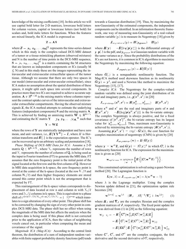
knowledge of the mixing coefficients [18]. In this article we willuse capital bold letter for 2-D matrices, lowercase bold lettersfor column vectors, capital or lowercase letters (not bold) forscalars and, bold italic letters for functions. When the featuresare mixed linearly, the ICA model is expressed as

where represents the time-series datasetwhich in this study is the complex-valued DCE-MRI datasetof a tumor or a tissue-mimicking phantom (observed mixtures)and N is the number of time points in the DCE-MRI sequence,

is a matrix containing the M structuresthat are known as independent components or ICs (usually MN) and in this study these are the images representing the in-

travascular and extravascular extracellular spaces of the tumortissue. Although we assume that there are only two spaces inour model (intravascular and extravascular extracellular), sinceICA makes no assumption about the spatial distribution of thesespaces, it might split each space into several components. Inpractice more than two ICs are required to achieve accurate sep-aration. is the mixing matrix whose columns repre-sent the contrast uptake curves of the intravascular and extravas-cular extracellular compartments. Having the observed mixturesignals , the ICA method attempts to estimate the underlyingfeatures (independent components) and the mixing matrix .This is achieved by finding an unmixing matrixand estimating the IC matrix such that

where the rows of are statistically independent and have zeromean, and unit variance, i.e., , where is Her-mitian transform and is the expectation operator. The IC’scan be recovered up to an arbitrary scaling and permutation [18].Phase Shifting of DCE-MRI Data for ICA: Assume a 2-D

matrix , where represents the number of rowsand represents the number of columns of , is being used asthe input to Fourier transform (FT) to generate the MRI data. FTassumes that the zero frequency point is the initial point of thesignal located at the first row and the first column of . Howeverin MRI data acquisition in k-space, the zero frequency point isstored at the center of the k-space (located at the row andcolumn ) and then higher frequency elements are storedaround this center point which is not the arrangement that isexpected by FT.This rearrangement of the k-space values corresponds to dis-

placement of data located at row n and column m withrows and columns in k-space. This is equivalent to a phaseshift of which trans-lates to a sign alteration of every other point. This phase shift hasto be corrected by changing the sign of every other point in com-plex DCE-MRI data. The phase shift has no effect when usingthe magnitude of the MRI data but affects the analysis when thecomplex data is being used. If this phase shift is not correctedprior to the application of ICA, then the values of neighboringvoxels cancel out, in particular when computing the mean andcovariance of the signal.Magnitude ICA (Mag-ICA): According to the central limit

theorem, the distribution of a sum of independent random vari-ableswithfinite support probability density functions (pdf) tends

towards a Gaussian distribution [19]. Thus, by maximizing thenon-Gaussianity of the estimated components, the independentcomponents can be identified. In an information theoretic frame-work, one way of measuring non-Gaussianity of a real-valuedrandom variable is to measure its Negentropy [18] given by

where is the differential entropy ofis the pdf, and is a Gaussian random variable with

the same variance as . Since the probability distributions of theICs are not known, it is common in ICA algorithms to maximizethe Negentropy by maximizing the following equation:

where is a nonquadratic nonlinearity function. TheMag-ICA method used skewness function as its nonlinearity

, and used a Newton like method to maximize theNegentropy [15], [17].Complex ICA: The Negentropy for the complex-valued

random variable was defined using the joint distribution of itsreal and imaginary parts, i.e., in [20]

where and are the real and imaginary parts of andis the bi-variate entropy.

The complex Negentropy is always positive, and for a fixedcovariance of , the bi-variate entropy has its largestvalue for . Thus, maximum non-Gaussianity isachieved by minimizing the bi-variate entropy .Assuming , the cost function for

complex maximization of negentropy (CMN) is given by [20]

where , and in which is thenonlinearity function for ICA. The expression for themaximiza-tion is given as [20]

This constrained optimization is solved using a quasi-Newtonmethod [20]. The Lagrangian function is

where is the Lagrange multiplier. Using the complexNewton update defined in [21], the optimization update rulebecomes [20]

(1)

where and are the complex Hessian and the complexgradient matrices of , respectively. The fixed point update forwas derived from (1) in [20] as the following equation:

where , , and are the complex conjugate, the firstderivative and the second derivative of , respectively.


B. Adaptive Complex ICA (AC-ICA)

The optimal non-Gaussianity in an information theo-retic framework is the logarithm of the joint probabilitydensity function of the source that is being estimated, i.e.,

. However, the joint proba-bility density of the source is not known in ICA and thus hasto be estimated.The generalized Gaussian distribution (GGD) is given as

(2)

where is the gamma function defined as, and and are the model parameters. The

GGD distribution covers a wide range of distributions [22]and has been used in modeling various physical phenomena[23]–[25].GGD was introduced in [22] as a cost function for ICA. We

have observed that distribution of the real and imaginary partsof the MR images of each compartment (source) fits well intothe GGD formulation. Assuming the linear mixture model holdsfor the MRI data in complex domain we modeled the MR imageas a sum of a number of functions with GGD distributions.Using an expectation maximization framework (explained in

the next section) the parameters of these GGD distributionsare found at each iteration and the GGD distribution with thehighest membership probability is used to derive the nonlin-earity in our ICA algorithm. Substituting the parametersof the selected GGD distribution in (2) and using the relation-ship between the ICA nonlinearity and the pdf of the sources,i.e., , the nonlinearity is defined as

C. Expectation Maximization

We developed an expectation maximization framework tocalculate the parameters of the adaptive probability distribu-tion by modeling the pdf of the estimated component as amixture of a number of GGD distributions at each iteration.Assuming the probability density function of the estimatedcomponent at each iteration, i.e., , is comprisedof k random variables with GGD distributions of the form

, and eachGGD contributes to formation of the pdf of with a member-ship probability we have

whereis the parameter space. is a probability density function,thus

is also a probability density function, therefore, and thus

and since are probabilities, they are nonnegative .The maximum Log-likelihood estimate can be formulated as

where N represents the number of samples in . The maximumlikelihood estimation is formulated as

defining , results in the fol-lowing conditional probabilities that are called membershipprobabilities:

using Jensen’s inequalities [26], i.e.,, the Log-likelihood at each iteration

can be expressed as

where is the lower bound for the Log-likelihood func-tion. Thus, to calculate the maximum Log-likelihood estimatorwe need to maximize its lower bound, iteratively

(3)

The second term of the right-hand side of (3) is a constant as it iscalculated from the old values. Thus, the maximization problemis simplified to

The probabilities can be calculated at each iterationusing

(4)


Setting the derivative of with respect to equal tozero we have

which results in the following expression for at each itera-tion

(5)

Setting the derivative of with respect to equal tozero we have

This equation results in (6) that will be used to calculate ateach iteration

(6)

where , is the polygamma function.This equation can be solved using any optimization algorithm.We used the fzero function of MATLAB (The MathWorks Inc.,Natick, MA, USA) software to find the value of at eachiteration.These three equations are solved at each iteration and the pa-

rameter set are calculated foreach GGD distribution. The GGD that has the highest member-ship probability was selected as the pdf of the sourceand its parameters were used in the ICA algorithm.

D. Simulation Phantom

A simulation study was conducted to simulate DCE-MR im-ages of a leaky phantom using a combination of finite elementanalysis (FEA) and classical description of MRI physics bymeans of Bloch equations.Leakage Model (Finite Element Analysis): The Comsol Mul-

tiphysics (Comsol Inc., Burlington, MA, USA) finite elementanalysis (FEA) software was used to construct the simulatedphantom that is shown in Fig. 1. This phantom is comprised ofa grid of 10 10 leaky tubes that run in parallel through a cubicchamber of agar gel (0.5% agar gel). The tubes have internal di-ameter of 200 , wall thickness of 30 and center to centerspacing of 300 . To model our experimental phantom exper-iments some of the tubes are removed to simulate the blockedor damaged tubes as shown in Fig. 1. The study simulated thepassage of a bolus of contrast agent through the tubes and itsleakage from the tubes into the agar gel over time. The spacingand diameter of the tubes were selected such that the vascular

Fig. 1. a: 3-D view of the simulation phantom, it also shows the imagingplane that is located halfway through the phantom in x-direction and lies in theyz-plane. b: The xz plane showing the tubes are parallel in the gel. c: The viewof the phantom from zy-plane that lies in the MR imaging plane.

fraction of the phantom is 3.8% so that it simulates the vascularvolume fraction of a tumor tissue [27].The 2-D DCE-MRI data was simulated for an imaging plane

half way through the length of the chamber, transverse to thephantom as depicted in Fig. 1(a). A cross-section showingthe orientation of the tubes in the imaging plane is shown inFig. 1(c). As the contrast agent arrives in the transverse plane itdiffuses into the surrounding gel. A range of different diffusioncoefficient was assigned to the gel, the tubes and tube wallsto account for variability of diffusion throughout the gel andgenerate a heterogeneous leakage apace. As such, the imagingplane was split into 2555 subdomains as shown in Fig. 2(a)with different diffusion coefficients. It was assumed that thediffusion coefficient of the gel had a uniform probability dis-tribution with mean value of mm [28] andstandard deviation of mm . The subdomainsthat constructed the inside of the tubes were given the highestdiffusion coefficients mm as they weresimulating flow of water and the subdomains corresponding tothe walls of the tubes were assigned the lowest diffusion coeffi-cients mm . The subdomains aroundone of the tubes showing the inner circle of the tube, the tubewall and the surrounding gel subdomains are also illustrated inFig. 1(a). The simulation was performed for 6.48 min with atemporal resolution of 3.3 s which was chosen according to ourexperimental study. The flow rate and contrast concentration ofthe simulated bolus that was applied to the tubes at theplane was selected such that the concentration-time curve of thetubes in the imaging plane was the same as our experimentalstudies. The contrast concentration distribution at time 2.5 minafter injection of the contrast agent is shown in Fig. 2(b) whichshows the heterogeneous distribution of contrast agent in thephantom.Dynamic Contrast Enhanced-MRI Simulation: It was as-

sumed that water was flowing through the tubes and the bolusof Gadolinium (Gd)-DTPA contrast agent is added to theflowing water. The geometry and contrast concentration of thetubes and the agar gel that were calculated in the FEA werefed to the developed MRI simulation software, and 120 frameswere simulated to generate the DCE-MRI dataset. This sectionprovides an overview of the 2-D MRI simulator that solved theBloch equation at each voxel. It was developed based on theSIMRI project which was developed to simulate MR images


Fig. 2. a: FE subdomains of the phantom in the imaging plane. There are 2555subdomains in this plane with different diffusion coefficients. As shown in theenlarged region of the phantom, the tubes, their walls and their surrounding gelareas are separated and proper diffusion coefficients are assigned to the sub-domains of each region. b: Contrast agent distribution in the imaging plane, attime min after injection of the contrast agent. This figure shows the het-erogeneous distribution of the contrast agent in the phantom.

[29]. The developed simulator starts with assigning protondensity , longitudinal relaxation , and transverse relaxationto each voxel; these parameters are necessary for computing

local spin magnetization. It was assumed that each voxel iscomprised of two isochromates [30] corresponding to the tubeand gel compartments.The proton density of each isochromate at each voxel was

calculated by taking the percentage of the voxel that belongedto the tubes/gel, which was available from the FEA step, multi-plied by the proton density of water/gel. The pre-contrast re-laxations of water and 0.5% agar gel were set to be 3000ms and 2100 ms respectively. The pre-contrast relaxations

of the water and gel were set to 250 ms and 65 ms, re-spectively, [29], [31]. The post-contrast and values werecalculated using the following equations [32]:

where and are the pre-contrast longitudinal and trans-verse relaxations, respectively, mm and

mm are the longitudinal and transverse relaxivitiesof contrast agent respectively and [Gd] is the contrast concen-tration of water/gel that was calculated in the FEA step for eachvoxel at each frame of the dynamic sequence. The use of twoisochromates in each voxel facilitates a realistic simulation ofthe cases where there are two different materials in the voxel. Italso allows for simulation of intra-voxel de-phasing of spins inthe voxel.The dynamic contrast-enhanced image simulation was

performed assuming a magnetic field of 1.5T with1 ppm inhomogeneity using a single coil RF pulse. 2-Dspoiled gradient recalled (SPGR) sequence of 120 framestemporal resolution were simulated. Other imagingparameters of the MRI simulation were: ms,ms, flip angle , band width kHz,

, field of view FOV mm,slice thickness mm. Gaussian noise was added to thek-space data and its standard deviation was selected such thatan SNR of 20 was achieved in image space.The simulated DCE-MRI data was reconstructed at four dif-

ferent resolutions. The high resolution dataset had in-plane res-

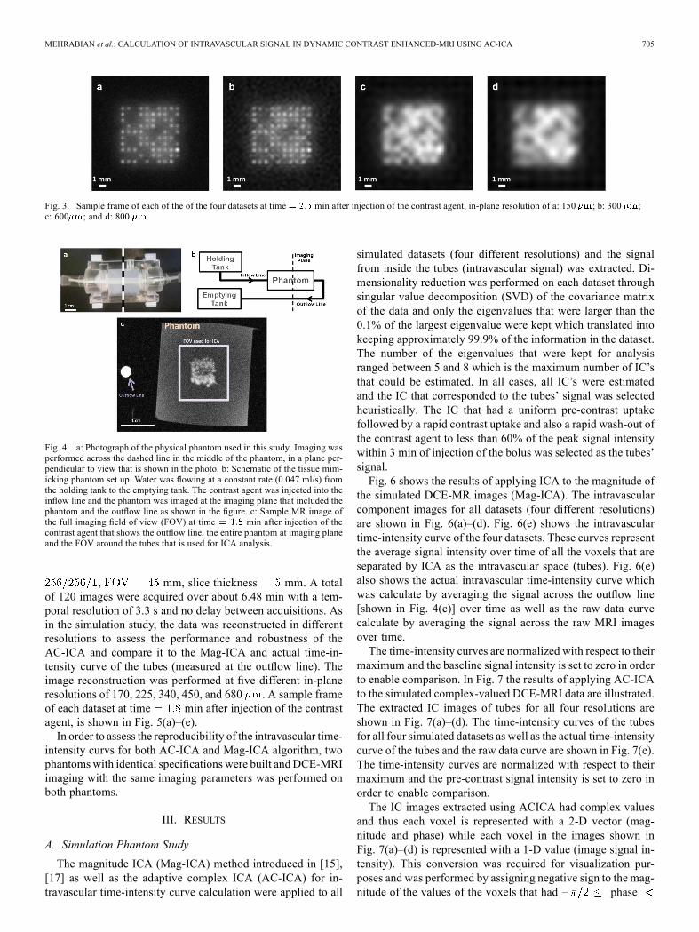
olution of 150 . In other datasets high frequency elementswere removed and the low resolution datasets had in-plane reso-lutions of 300, 600, and 800 . A sample frame of each datasetat time min after injection of the contrast agent is shownin Fig. 3.The magnitude of the MRI data is usually used in PK anal-

ysis of tumors. Thus, the performance of the proposed adaptivecomplex ICA (AC-ICA) intravascular signal calculation tech-nique was compared to the case in which ICA was applied tothe magnitude of the MRI data (magnitude ICA or Mag-ICA).The use of DCE-MRI data with different resolutions was alsoused to assess the robustness of the AC-ICA technique in sep-arating intravascular signal, particularly in low resolutions thatare more commonly encountered in clinical trials.Since ICA is a stochastic process, it is important to assess

the reproducibility of the intravascular time-intensity curves.Therefore, to assess the reproducibility of the AC-ICA andMag-ICA results, the DCE-MRI dataset at each resolution wasgenerated five times. Although these datasets were generatedwith the same imaging, geometry and physical parameters, theydiffered in distribution of inhomogeneity that was addedto the main magnetic field as a random Gaussian signal (1ppm inhomogeneity) and the Gaussian noise thatwas added to the data. The Gaussian noise was added to thesimulated k-space data where standard deviation of noise wasselected such that the SNR in image space was 20 .

E. Tissue Mimicking Phantom

A physical phantom, similar to the simulation phantom, wasconstructed that consisted of a chamber of agar gel (0.5 wt%,Sigma-Aldrich Canada Ltd., Oakville, ON, Canada) used astissue mimicking material and a grid of 10 10 dialysis tubing(Diapes PES-150, Baxter) representing the vascular component.These tubes that approximated the diameter of small arteriesor large arterioles had inner diameter of 200 , wall thick-ness of 30 and center to center spacing of 300 andpassed through the agar gel parallel to each other, as shown inFig. 4(a). These porous tubes (pore size of 89–972 nm) allowedlow-molecular weight contrast agent to freely diffuse from thetubes into the agar gel.DCE-MR imaging was performed at a transverse plane in

the middle of the phantom, as shown in Fig. 4(a). Water wasflowing through the tubes and an MR image of the phantomat the imaging plane is shown in Fig. 4(b). The gadolinium(Gd)-DTPA contrast agent was injected to the water stream asa bolus. Once the bolus reached the chamber that containedthe gel, it was capable of leaking from the tubes into the gel.The flow of water was kept at a constant rate of 0.047 ml/swhich translates into a flow velocity within arteriole’s physi-ological range [33]. In order to measure the contrast agent con-centration inside the tubes, the outflow line of the flow was ori-ented such that it passed through the imaging plane as shown inFig. 4(b) and (c). The MR signal of this outflow line was usedas the actual tubes’ signal (with a delay of 9.7 s) and was usedto validate the calculated intravascular time-intensity curve.Dynamic contrast-enhanced imaging was performed using a

2-D fast spoiled gradient recalled (fSPGR) sequence with thefollowing imaging parameters: ms, ms,flip angle , kHz,


Fig. 3. Sample frame of each of the of the four datasets at time min after injection of the contrast agent, in-plane resolution of a: 150 ; b: 300 ;c: 600 ; and d: 800 .

Fig. 4. a: Photograph of the physical phantom used in this study. Imaging wasperformed across the dashed line in the middle of the phantom, in a plane per-pendicular to view that is shown in the photo. b: Schematic of the tissue mim-icking phantom set up. Water was flowing at a constant rate (0.047 ml/s) fromthe holding tank to the emptying tank. The contrast agent was injected into theinflow line and the phantom was imaged at the imaging plane that included thephantom and the outflow line as shown in the figure. c: Sample MR image ofthe full imaging field of view (FOV) at time min after injection of thecontrast agent that shows the outflow line, the entire phantom at imaging planeand the FOV around the tubes that is used for ICA analysis.

, mm, slice thickness mm. A totalof 120 images were acquired over about 6.48 min with a tem-poral resolution of 3.3 s and no delay between acquisitions. Asin the simulation study, the data was reconstructed in differentresolutions to assess the performance and robustness of theAC-ICA and compare it to the Mag-ICA and actual time-in-tensity curve of the tubes (measured at the outflow line). Theimage reconstruction was performed at five different in-planeresolutions of 170, 225, 340, 450, and 680 . A sample frameof each dataset at time min after injection of the contrastagent, is shown in Fig. 5(a)–(e).In order to assess the reproducibility of the intravascular time-

intensity curvs for both AC-ICA and Mag-ICA algorithm, twophantomswith identical specifications were built andDCE-MRIimaging with the same imaging parameters was performed onboth phantoms.

III. RESULTS

A. Simulation Phantom Study

The magnitude ICA (Mag-ICA) method introduced in [15],[17] as well as the adaptive complex ICA (AC-ICA) for in-travascular time-intensity curve calculation were applied to all

simulated datasets (four different resolutions) and the signalfrom inside the tubes (intravascular signal) was extracted. Di-mensionality reduction was performed on each dataset throughsingular value decomposition (SVD) of the covariance matrixof the data and only the eigenvalues that were larger than the0.1% of the largest eigenvalue were kept which translated intokeeping approximately 99.9% of the information in the dataset.The number of the eigenvalues that were kept for analysisranged between 5 and 8 which is the maximum number of IC’sthat could be estimated. In all cases, all IC’s were estimatedand the IC that corresponded to the tubes’ signal was selectedheuristically. The IC that had a uniform pre-contrast uptakefollowed by a rapid contrast uptake and also a rapid wash-out ofthe contrast agent to less than 60% of the peak signal intensitywithin 3 min of injection of the bolus was selected as the tubes’signal.Fig. 6 shows the results of applying ICA to the magnitude of

the simulated DCE-MR images (Mag-ICA). The intravascularcomponent images for all datasets (four different resolutions)are shown in Fig. 6(a)–(d). Fig. 6(e) shows the intravasculartime-intensity curve of the four datasets. These curves representthe average signal intensity over time of all the voxels that areseparated by ICA as the intravascular space (tubes). Fig. 6(e)also shows the actual intravascular time-intensity curve whichwas calculate by averaging the signal across the outflow line[shown in Fig. 4(c)] over time as well as the raw data curvecalculate by averaging the signal across the raw MRI imagesover time.The time-intensity curves are normalized with respect to their

maximum and the baseline signal intensity is set to zero in orderto enable comparison. In Fig. 7 the results of applying AC-ICAto the simulated complex-valued DCE-MRI data are illustrated.The extracted IC images of tubes for all four resolutions areshown in Fig. 7(a)–(d). The time-intensity curves of the tubesfor all four simulated datasets as well as the actual time-intensitycurve of the tubes and the raw data curve are shown in Fig. 7(e).The time-intensity curves are normalized with respect to theirmaximum and the pre-contrast signal intensity is set to zero inorder to enable comparison.The IC images extracted using ACICA had complex values

and thus each voxel is represented with a 2-D vector (mag-nitude and phase) while each voxel in the images shown inFig. 7(a)–(d) is represented with a 1-D value (image signal in-tensity). This conversion was required for visualization pur-poses and was performed by assigning negative sign to the mag-nitude of the values of the voxels that had phase


Fig. 5. Sample frame of each of the five experimental DCE-MRI datasets of the phantom at time min after injection of the contrast agent, with in-planeresolutions of: a: 170 ; b: 225 ; c: 340 ; d: 450 ; and e: 680 .

Fig. 6. The separated tubes image and the time-intensity curve of the tubes calculated using Mag-ICA for each of the four simulated DCE-MRI datasets. Tubesimages for datasets with in-plane resolutions of a: 150 ; b: 300 ; c: 600 ; d: 800 . e: Calculated time-intensity curves of the tubes corresponding tothe four simulated datasets, the Actual time-intensity curve of the tubes and the curve corresponding to the mean across the entire raw (not analyzed) images overtime (raw data).

and assigning positive sign to the magnitude of the valuesof the voxel with phase or phase . This methodof visualizing the images provides consistent results with theMag-ICA analysis where we had both negative and positivesignal intensity values.For each in-plane resolution, five DCE-MRI data sets of the

phantom were simulated with . The AC-ICA andMag-ICA algorithms were applied to all datasets. Table I reportsthe root mean square error (RMSE) between the estimated time-intensity curves of the tubes obtained using each algorithm andthe actual curve for all four datasets. Table I also reports thecorrelation coefficient between the estimated and actual time-intensity curves of the tubes for both algorithms.

B. Experimental Phantom Study

The adaptive complex ICA and magnitude ICA were also ap-plied to DCE-MRI images of the experimental tissue mimicking

phantom. Similar to the simulation study, dimensionality reduc-tions was performed first, where eigenvalues that were largerthat 0.1% of the largest eigenvalue were kept. The phantomdata was reconstructed in five different in-plane resolutions andboth algorithms were applied to all five datasets. Fig. 8 showsthe results of applying the Mag-ICA algorithm to the exper-imental DCE-MRI data. The IC images corresponding to thetubes’ signal of the five datasets are shown in Fig. 8(a)–(e). Thetime-intensity curves of the five datasets as well as the actualtime-intensity curve of the tubes that was measured at the out-flow line of the phantom and the raw data curve calculate byaveraging the signal across the raw MRI images over time areshown in Fig. 8(f). The baseline values of the time-intensitycurves of all datasets were set to zero and they were normal-ized with respect to their maximum values.Fig. 9 shows the results of applying the proposed AC-ICA

algorithm to the DCE-MRI data of the experimental phantom


Fig. 7. The separated tubes image and the time-intensity curve of the tubes calculated using AC-ICA for each of the four simulated DCE-MRI datasets. Tubesimages for datasets with in-plane resolutions of a: 150 ; b: 300 ; c: 600 ; d: 800 . e: Calculated time-intensity curves of the tubes corresponding tothe four simulated datasets, the Actual time-intensity curve of the tubes and the curve corresponding to the mean across the entire raw (not analyzed) images overtime (raw data).

TABLE IROOT MEAN SQUARE ERROR (RMSE) AND CORRELATION COEFFICIENTBETWEEN THE ESTIMATED TUBES’ TIME-INTENSITY CURVES AND THEACTUAL CURVE FOR FOUR DATASET IN BOTH ICA ALGORITHMS (RMSEAND CORRELATION COEFFICIENTS ARE CALCULATED AFTER SETTING THEBASELINE VALUES OF THE CURVES TO ZERO AND NORMALIZING THEM)

for all five different in-plane resolutions. The separated tubes’images of the five datasets are shown in Fig. 9(a)–(e). The corre-sponding time-intensity curves of the tubes in these datasets aswell as the actual time-intensity curve of the tubes measured atthe outflow curve of the phantom and the raw data curve areshown in Fig. 9(f). The baseline values of the time-intensity

curves of all datasets were set to zero and they were normal-ized with respect to their maximum values.Two experimental phantoms were built and DCE-MRI

imaging was performed on both phantoms to assess the repro-ducibility of the results for both intravascular time-intensitycurve calculation algorithms. Table II reports the root meansquare error (RMSE) between the estimated and the actualtime-intensity curves of the tubes (outflow) for all five datasetsof both phantoms. This table also reports the correlation coeffi-cient between the estimated and actual time-intensity curves ofthe tubes for both algorithms in all five in-plane resolutions.

IV. DISCUSSIONS

Measurements of tumor size and serum markers are not ef-ficient criteria in assessing tumor response to therapy partic-ularly in anti-angiogenic therapies. Pharmacokinetic modelingof DCE-MR images of a tumor is one of the approaches usedto assess its therapeutic response. A fundamental step in PKmodeling that is common amongst most models is determiningthe intravascular contrast agent concentration which is approx-imated using an arterial input function (AIF). Mehrabian et al.[15], [17] developed an ICA-based method to measure and sep-arate signal that is generated in the tumor vasculature. Althoughthe output of MR imaging is complex-valued, only the magni-tude data was used (as is common in most DCE-MRI studies)and the phase information was not utilized in the study. This in-troduced a fundamental challenge in ICA analysis as the linear


Fig. 8. The separated tubes image and the time-intensity curve of the tubes calculated using Mag-ICA for each of the five experimental DCE-MRI datasets of thetissue mimicking phantom. Tubes images for datasets with in-plane resolutions of a: 170 ; b: 225 ; c: 340 ; d: 450 ; and e: 680 . e) Calculatedtime-intensity curves of the tubes corresponding to the five experimental datasets, the Actual time-intensity curve of the tubes (outflow) and the curve correspondingto the mean across the entire raw (not analyzed) images over time (raw data).

mixture assumption of ICA was violated. This problem was ad-dressed by using short echo time (TE) and minimizing intra-voxel de-phasing [15], [17]. The separated intravascular imageand time-intensity curves were validated against intravascularcontrast enhanced ultrasound measurements in both phantomsand animal models.An adaptive complex ICA (AC-ICA) method was introduced

in this study that used the complex-valued MRI data for ICAand also used an adaptive cost function for ICA. The adaptivecost function was determined by assuming the probability dis-tribution of MRI data takes the form of a mixture of general-ized Gaussian distributions (GGD) whose parameters were esti-mated using an expectation maximization (EM) approach. Sim-ulated and experimental phantoms were constructed and theirtheoretical and experimental DCE-MRI data were acquired re-spectively. Each phantomwas comprised of a grid of leaky tubesthat represented the tumor vasculature embedded in a chamberof agar gel that represented the extravascular extracellular spaceof the tumor.The AC-ICA method was applied to the DCE-MRI data of

simulated and experimental phantoms and the tubes’ time-in-tensity signal was estimated. These results were compared withthe results of calculating time-intensity curves of the tubes usingthe Mag-ICA method that was introduced in [15], [17] to high-light the better performance of the AC-ICA. Both experimentaland simulation data where reconstructed in different resolutionsto assess the robustness of the method and its capability in sep-arating signal of the tubes in low resolution data that are morecommon in clinical practice.

As shown in Figs. 6 and 7, and Table I, in simulation studyboth AC-ICA and Mag-ICA methods were capable of sepa-rating time-intensity curve of the tubes with high accuracy forhigh resolution data in both spatial and temporal domains. Asthe voxel size increased (lower resolution), the AC-ICA demon-strated higher accuracy and robustness compared toMag-ICA indealing with datasets with a wide range of in-plane resolutions.There were small differences between the time-intensity curvesof the tubes calculated using AC-ICA for different resolutionswhile Mag-ICA curves changed significantly and its time-inten-sity curves were not good for the lower resolutions. Note that inlower resolutions although the tubes could not be visualized inthe spatial domain, however; their time-intensity curve was cal-culated with good accuracy.Similar results were obtained in the experimental DCE-MRI

data as shown in Figs. 8 and 9 and reported in Table II. Thetubes were separated accurately in both spatial and temporal do-mains for the high resolution data. As the pixel size increasedit became more difficult to visualize the tube in the IC imagessuch that in the two lowest resolutions it was impossible to seethem separately from the leakage. However the time-intensitycurve of the tubes was estimated with high accuracy for all res-olutions in both AC-ICA and Mag-ICA methods. Similar to thesimulation studies, the AC-ICA demonstrated better accuracy indealing with lower resolution data and there were smaller dif-ferences between time-intensity curves of the tubes at varyingresolutions compared to the Mag-ICA.There was an aura in the experimental phantom images out-

side of the tubes which is due to fabrication artifact. A few of


Fig. 9. The separated tubes image and the intravascular time-intensity curve of the tubes calculated using AC-ICA for each of the five experimental DCE-MRIdatasets of the tissue mimicking phantom. Tubes images for datasets with in-plane resolutions of a) 170 ; b) 225 ; c) 340 ; d) 450 ; and e) 680 . e)Calculated time-intensity curves of the tubes corresponding to the five experimental datasets, the Actual time-intensity curve of the tubes (outflow) and the curvecorresponding to the mean across the entire raw (not analyzed) images over time (raw data).

TABLE IIRMSE AND THE CORRELATION COEFFICIENT BETWEEN THE ESTIMATED

AND ACTUAL TIME-INTENSITY CURVES OF THE TUBES (OUTFLOW) FOR ALLFIVE DATASETS OF BOTH PHANTOMS FOR MAG-ICA AND AC-ICA (RMSEAND CORRELATION COEFFICIENTS ARE CALCULATED AFTER SETTING THE

BASELINE OF THE CURVES TO ZERO AND NORMALIZING THEM)

the tubes were broken during the phantom construction processand the contrast agent was capable of leaving these broken tubesmore easily. The results show that this aura is smaller in thetubes image of the ACICA analysis (particularly in the high-res-olution images) compared to the Mag-ICA results which shows

that ACICA is capable of separating the intravascular spacemore accurately.There are two reasons for superior performance of AC-ICA:

1) the ICA cost function is adapted at every iteration to matchthe probability distribution of the tubes’ signal, 2) unlike theMag-ICA, the linear mixture assumption of ICA is not violatedin AC-ICA and thus intra-voxel de-phasing (spins inside eachvoxel are not necessarily in-phase) and partial volume effect donot play as significant role as they do in Mag-ICA.Moreover, in the experimental study the signal intensity of

the tubes dropped below its baseline value. This effect is cur-rently under investigation, however it could be associated withthe effects of the contrast agent that leaked to the EES on thevalue of the voxels inside the tubes. It could also be associatedwith the effects of the contrast agent that diffused too far fromthe tubes, such that it could not return to the tubes and could notbe washed out.In this study we developed an adaptive complex ICA-based

method to calculate and separate the intravascular signal inDCE-MRI datasets. However, in PK analysis of tumor tis-sues, this signal intensity has to be converted into contrastagent concentration. This is not a trivial step for the results ofICA-based method and requires further investigation as thereis an arbitrary scaling of the ICA results.It was shown that although the tubes were not visible in

the IC images of low resolution datasets (both simulation andexperiment), the intravascular time-intensity curves in low res-olution datasets are very close to the high resolution ones. This


demonstrates that ICA-based calculation of the intravasculartime-intensity curve has the potential to be used in clinicalstudies, where the resolution of DCE-MRI data is very low.The AC-ICA method provided more accurate results comparedto Mag-ICA which suggests that complex-valued (magnitudeand phase) DCE-MRI data should be used to calculate theintravascular time-intensity curve in the tumor. This could leadto more accurate PK analysis and better understanding of thetumor response to therapy.

REFERENCES[1] C. H. Lee, L. Braga, R. O. de Campos, and R. C. Semelka, “Hepatic

tumor response evaluation by MRI,” NMR Biomed., vol. 24, no. 6, pp.721–733, 2011.

[2] W. A. Weber, “Assessing tumor response to therapy,” J. Nucl. Med.,vol. 50, pp. 1S–10S, 2009, Suppl. 1.

[3] J. J. Smith, A. G. Sorensen, and J. H. Thrall, “Biomarkers in imaging:Realizing radiology’s future,” Radiology, vol. 227, no. 3, pp. 633–638,2003.

[4] M. Kanematsu, S. Osada, N. Amaoka, S. Goshima, H. Kondo, H. Kato,H. Nishibori, R. Yokoyama, H. Hoshi, and N. Moriyama, “Expres-sion of vascular endothelial growth factor in hepatocellular carcinomaand the surrounding liver and correlation with MRI findings,” Am. J.Roentgenol., vol. 184, no. 3, pp. 832–841, 2005.

[5] M. O. Leach, K. M. Brindle, J. L. Evelhoch, J. R. Griffiths, M. R.Horsman, A. Jackson, G. Jayson, I. R. Judson, M. V. Knopp, R. J.Maxwell, D.McIntyre, A. R. Padhani, P. Price, R. Rathbone, G. Rustin,P. S. Tofts, G. M. Tozer, W. Vennart, J. C. Waterton, S. R. Williams,and P.Workman, “Assessment of antiangiogenic and antivascular ther-apeutics using MRI: Recommendations for appropriate methodologyfor clinical trials,” Br. J. Radiol., vol. 76, pp. S87–S91, 2003.

[6] J. H. Naish, L. E. Kershaw, D. L. Buckley, A. Jackson, J. C. Waterton,and G. J. M. Parker, “Modeling of contrast agent kinetics in the lungusing T(1)-weighted dynamic contrast-enhanced MRI,” Magn. Reson.Med., vol. 61, no. 6, pp. 1507–1514, Jun. 2009.

[7] P. S. Tofts and A. G. Kermode, “Measurement of the blood-brain-bar-rier permeability and leakage space using dynamic MR imaging.1. Fundamental-concepts,” Magn. Reson. Med., vol. 17, no. 2, pp.357–367, 1991.

[8] H. L.M. Cheng, “Investigation and optimization of parameter accuracyin dynamic contrast-enhanced MRI,” J. Magn. Reson. Imag., vol. 28,no. 3, pp. 736–743, 2008.

[9] A. E. Hansen, H. Pedersen, E. Rostrup, and H. B. W. Larsson,“Partial Volume Effect (PVE) on the Arterial Input Function (AIF)in T-1-weighted perfusion imaging and limitations of the multiplica-tive rescaling approach,” Magn. Reson. Med., vol. 62, no. 4, pp.1055–1059, 2009.

[10] D. M. McGrath, D. P. Bradley, J. L. Tessier, T. Lacey, C. J. Taylor, andG. J. M. Parker, “Comparison of model-based arterial input functionsfor dynamic contrast-enhanced MRI in tumor bearing rats,” Magn.Reson. Med., vol. 61, no. 5, pp. 1173–1184, 2009.

[11] R. Lawaczeck, G. Jost, and H. Pietsch, “Pharmacokinetics of contrastmedia in humans model with circulation, distribution, and renal excre-tion,” Invest. Radiol., vol. 46, no. 9, pp. 576–585, Sep. 2011.

[12] D. A. Kovar, M. Lewis, and G. S. Karczmar, “A new method forimaging perfusion and contrast extraction fraction: Input functionsderived from reference tissues,” J. Magn. Reson. Imag., vol. 8, no. 5,pp. 1126–1134, 1998.

[13] A. Shukla-Dave, N. Lee, H. Stambuk, Y. Wang, W. Huang, H. T.Thaler, S. G. Patel, J. P. Shah, and J. A. Koutcher, “Average arterialinput function for quantitative dynamic contrast enhanced magneticresonance imaging of neck nodal metastases,” BMC Med. Phys., vol.9, p. 4, 2009.

[14] X. Fan, C. R. Haney, D. Mustafi, C. Yang, M. Zamora, E. J.Markiewicz, and G. S. Karczmar, “Use of a reference tissue and bloodvessel to measure the arterial input function in DCEMRI,” Magn.Reson. Med., vol. 64, no. 6, pp. 1821–1826, Dec. 2010.

[15] H. Mehrabian, C. Chandrana, I. Pang, R. Chopra, and A. L. Martel,“Arterial input function calculation in dynamic contrast-enhancedMRI: An in vivo validation study using co-registered contrast-en-hanced ultrasound imaging,” Eur. Radiol., vol. 22, no. 8, pp.1735–1747, 2012.

[16] J. G. Korporaal, M. Van Vulpen, C. A. T. Van Den Berg, and U. A.Van Der Heide, “Tracer kinetic model selection for dynamic contrast-enhanced computed tomography imaging of prostate cancer,” Invest.Radiol., vol. 47, no. 1, pp. 41–48, 2012.

[17] H. Mehrabian, I. Pang, C. Chandrana, R. Chopra, and A. L. Martel,“Automatic mask generation using independent component analysis indynamic contrast enhanced-MRI,” in Proc. Int. Symp. Biomed. Imag.,2011, pp. 1657–1661.

[18] P. Comon, “Independent component analysis, A new concept?,” SignalProcess., vol. 36, no. 3, pp. 287–314, 1994.

[19] A. Araujo and E.Giné, The Central Limit Theorem for Real and BanachValued Random Variables. NY: Wiley, 1980.

[20] M. Novey and T. Adali, “Complex ICA by negentropy maximization,”IEEE Trans. Neural Netw., vol. 19, no. 4, pp. 596–609, Apr. 2008.

[21] A. van den Bos, “Complex gradient and Hessian,” in IEE Proc Vis.Image Signal Proc., 1994, vol. 141, no. 6, pp. 380–382.

[22] M. Novey and T. Adalt, “Adaptable nonlinearity for complex max-imization of nongaussianity and a fixed-point algorithm,” in Proc.2006 16th IEEE Signal Process. Soc. Workshop Mach. Learn. SignalProcess., 2007, pp. 79–84.

[23] O. Bernard, J. D’hooge, and D. Friboulet, “Statistical modeling of theradio-frequency signal in echocardiographic images based on gener-alized Gaussian distribution,” in Proc. 3rd IEEE Int. Symp. Biomed.Imag.: From Nano to Macro, 2006, pp. 153–156.

[24] M. S. Davis, P. Bidigare, and D. Chang, “Statistical modeling andML parameter estimation of complex SAR imagery,” in Conf. Rec.—Asilomar Conf. Signals, Syst. Comput., 2007, pp. 500–502.

[25] D. Gonzalez-Jimenez, F. Perez-Gonzalez, P. Comesana-Alfaro, L.Perez-Freire, and J. L. Alba-Castro, “Modeling Gabor coefficientsvia generalized Gaussian distributions for face recognition,” in Proc.IEEE Int. Conf. Image Process., 2007, vol. 4, pp. 485–488.

[26] W. Rudin, Real and Complex Analysis. New York: McGraw-Hill,1987.

[27] A. Wall, T. Persigehl, P. Hauff, K. Licha, M. Schirner, S. Muller, A.von Wallbrunn, L. Matuszewski, W. Heindel, and C. Bremer, “Dif-ferentiation of angiogenic burden in human cancer xenografts using aperfusion-type optical contrast agent (SIDAG),” Breast Cancer Res.,vol. 10, 2008.

[28] T. S. Koh, S. Hartono, C. H. Thng, T. K. H. Lim, L. Martarello, andQ. S. Ng, “In vivo measurement of gadolinium diffusivity by dynamiccontrast-enhanced MRI: A preclinical study of human xenografts,”Magn. Reson. Med., vol. 69, no. 1, pp. 269–276, 2013.

[29] H. Benoit-Cattin, G. Collewet, B. Belaroussi, H. Saint-Jalmes, and C.Odet, “The SIMRI project: A versatile and interactive MRI simulator,”J. Magn. Reson., vol. 173, no. 1, pp. 97–115, 2005.

[30] P. Latta, M. L. H. Gruwel, V. Jellúš, and B. Tomanek, “Bloch simula-tions with intra-voxel spin dephasing,” J. Magn. Reson., vol. 203, no.1, pp. 44–51, 2010.

[31] L. Cochlin, A. Blamire, and P. Styles, “Dependence of T1 and T2 onhigh field strengths in doped agarose gels; facilitating selection of com-position for specific T1/T2 at relevant field,” Int. Soc. Magn. Reson.Med., p. 885, 2003.

[32] R. Hendrick and E. Haacke, “Basic physics of MR contrast agents andmaximization of image-contrast,” J. Magn. Reson. Imag., vol. 3, no. 1,pp. 137–148, 1993.

[33] W. A. Ritschel and G. L. Kearns, Handbook of Basic Pharmacoki-netics—Including Clinical Applications. Washington, D.C.: Am.Pharmaceutical Assoc., 1999.

ieee transactions on medical imaging, vol. 32, no. 4

Documents