ieee transactions on nanobioscience, vol. 11, no. 3...

IEEE TRANSACTIONS ON NANOBIOSCIENCE, VOL. 11, NO. 3, SEPTEMBER 2012 191

Inferred Spoligoforest Topology Unravels SpatiallyBimodal Distribution of Mutations in the DR RegionCagri Ozcaglar, Amina Shabbeer, Natalia Kurepina, Nalin Rastogi, Bülent Yener, and Kristin P. Bennett*

Abstract—Biomarkers of Mycobacterium tuberculosis complex(MTBC) mutate over time. Among the biomarkers of MTBC,spacer oligonucleotide type (spoligotype) and mycobacteriuminterspersed repetitive unit (MIRU) patterns are commonly usedto genotype clinical MTBC strains. In this study, we presentan evolution model of spoligotype rearrangements using MIRUpatterns to disambiguate the ancestors of spoligotypes. We use alarge patient dataset from the United States Centers for DiseaseControl and Prevention (CDC) to generate this model. Basedon the contiguous deletion assumption and rare observation ofconvergent evolution, we first generate the most parsimoniousforest of spoligotypes, called a spoligoforest, using three geneticdistance measures. An analysis of topological attributes of thespoligoforest and number of variations at the direct repeat (DR)locus of each strain reveals interesting properties of deletions inthe DR region. First, we compare our mutation model to existingmutation models of spoligotypes and find that our mutation modelproduces as many within-lineage mutation events as other models,with slightly higher segregation accuracy. Second, based on ourmutation model, the number of descendant spoligotypes followsa power law distribution. Third, contrary to prior studies, thepower law distribution does not plausibly fit to the mutation lengthfrequency. Moreover, we find that the total number of mutationevents at consecutive spacers follows a spatially bimodal distribu-tion. The two modes are spacers 13 and 40, which are hotspots forchromosomal rearrangements, and the change point is spacer 34,which is absent in most MTBC strains. Based on this observation,we built two alternative models for mutation length frequency:the Starting Point Model (SPM) and the Longest Block Model(LBM). Both models are plausibly good fits to the mutation lengthfrequency distribution, as verified by the goodness-of-fit test. Wealso apply SPM and LBM to a dataset from Institut Pasteur deGuadeloupe and verify that these models hold for different straindatasets.Index Terms—DR region, MIRU-VNTR, mutation model, My-

cobacterium tuberculosis complex, spoligotype, tuberculosis.

I. INTRODUCTION

T UBERCULOSIS (TB) is a leading cause of death amonginfectious diseases. Tuberculosis is caused by Mycobac-

terium tuberculosis complex (MTBC). One third of the human

Manuscript received July 10, 2012; accepted August 01, 2012. Date of currentversion September 10, 2012. This work was supported by NIH R01LM009731.Asterisk indicates corresponding author.C. Ozcaglar, A. Shabbeer, and B. Yener are with the Computer Science

Department, Rensselaer Polytechnic Institute, Troy, NY 12180 USA (e-mail:[email protected]; [email protected]; [email protected]).N. Kurepina is with the TB Center, Public Health Research Institute, Newark,

NJ 07103 USA (e-mail: [email protected]).N. Rastogi is with the Tuberculosis andMycobacteria Unit, Institut Pasteur de

Guadeloupe, 97183 Abymes Cedex, France (e-mail: [email protected]).*K. P. Bennett is with the Computer Science Department and Mathematical

Sciences Department, Rensselaer Polytechnic Institute, Troy, NY 12180 USA(e-mail: [email protected]).Color versions of one or more of the figures in this paper are available online

at http://ieeexplore.ieee.org.Digital Object Identifier 10.1109/TNB.2012.2213265

population is infected, either latently or actively, with TB [1].DNA fingerprinting of MTBC strains is used for tracking thetransmission of tuberculosis. Isolates from TB patients aregenotyped using multiple biomarkers, which include spaceroligonucleotide types (spoligotypes), mycobacterium inter-spersed repetitive units—variable number tandem repeats(MIRU-VNTR), and IS6110 restriction fragment length poly-morphism (RFLP) [2]–[4].Biomarkers of MTBC change over time. Brosch et al. pre-

sented an evolutionary repetition model based on the analysisof twenty regions of difference (RD) found in a comparisonof whole genome sequences of MTBC clinical strains [5], [6].Tanaka et al. introduced cluster-graphs to analyze genotypeclusters of MTBC separated by a single mutation step [7].Based on the observation that deletion length follows a Zipfdistribution, Reyes et al. presented a probabilistic mutationmodel of spoligotypes to disambiguate the ancestors [8]. Grantet al. simulated stepwise loss or gain of repeats in MIRU lociusing a stochastic continuous-time model, and suggested thatall MIRU loci mutate very slowly [9].In this study, we present a mutation model of spoligotypes

based on variations in the direct repeat (DR) region. To disam-biguate the parents in the cluster-graph, we add an independentbiomarker, MIRU-VNTR. First, we use a large patient datasetfrom the United States Centers for Disease Control and Pre-vention (CDC) and generate the most parsimonious forest ofspoligotypes, called a spoligoforest. The spoligoforest genera-tion is based on the contiguous deletion assumption, nonexis-tence of convergent evolution and three distance measures de-fined on spoligotypes and MIRU patterns. The spoligoforestof the CDC dataset in Fig. 1 generated using this model dis-plays the putative history of mutation events in the chromo-somal DR region. Each node in the spoligoforest represents adistinct spoligotype, and each edge represents a potential mu-tation event from parent spoligotype to child spoligotype. Thenumber of spacers lost in a mutation event is referred as the mu-tation length. We compare the DR evolution model to existingmutation models in terms of number of mutations and segrega-tion accuracy and show that our mutation model with the ad-ditional biomarker, MIRU-VNTR, leads to as many within-lin-eage mutation events as in other mutation models. We identi-fied topological attributes of the spoligoforest and gave insightsinto variations of spoligotypes. Based on the spoligoforest, thenumber of descendant spoligotypes follows a power law distri-bution. On the other hand, based on goodness-of-fit results, themutation length frequency does not follow a power law distri-bution, in contrast to prior studies. The number of mutationsat contiguous DR loci follows a bimodal distribution, and the

1536-1241/$31.00 © 2012 IEEE

192 IEEE TRANSACTIONS ON NANOBIOSCIENCE, VOL. 11, NO. 3, SEPTEMBER 2012

Fig. 1. The spoligoforest of the CDC dataset. Each node represents a distinct spoligotype, and each edge represents a one-step mutation event from parent spoligo-type to child spoligotype. Node sizes are proportional to the number of patients infected with MTBC strains having the spoligotype, in log scale. Nodes are coloredby major lineages of MTBC strains. The spoligoforest generator is implemented in Java, using the visualization software Graphviz [10].

modes are spacer 13 and spacer 40, which are hotspots, e.g.,sites of increased observed variability. Spacer 34 is the changepoint in the distribution, and it is stable, which is due to lack ofspacers 33–36 in most MTBC strains in the CDC dataset. Wehypothesized that this bimodal distribution results in unobserv-able longer mutation events, which is why power law distribu-tion is not a plausible fit to mutation length frequency. Based onthis observation, we built two alternative models for mutationlength frequency. The Starting Point Model (SPM) conditionsthe mutation length on the starting point of mutation, and theLongest Block Model (LBM) conditions the mutation length onthe length of the longest contiguous block spacers beyond thestarting point of mutation. Both SPM and LBM are plausiblygood models for mutation length frequency distribution.

II. BACKGROUND

In order to build a mutation model for evolution of the chro-mosomal DR region, we used two biomarkers ofMTBC: spolig-otypes and MIRU patterns. Each biomarker has a different mu-tation mechanism which is analyzed separately. Spoligotypescan lose spacers in the DR region, but not gain, whileMIRU locican either lose or gain tandem repeats [11]–[13]. In this section,we give a brief background on spoligotyping, MIRU-VNTRtyping, and mutation of both biomarkers.

A. Spoligotyping

Spoligotyping is a PCR-based genotyping method of MTBCthat exploits the polymorphism in the DR locus. The DRregion belongs to the class of clustered regularly interspaced

palindromic repeats (CRISPR) loci [14]. It comprises directlyrepeating sequences of 36 bp, separated by unique spacersequences of 36 to 41 bp [15]. One repeat sequence and thefollowing spacer sequence together is termed a direct variablerepeat (DVR). A spoligotype is composed of 43 spacers, whichare represented by a 43-bit binary sequence, where zeros andones indicate absence and presence of particular spacer in theDR locus respectively.

B. MIRU-VNTR Typing

MIRU is a homologous 46–100 bp DNA sequence tandemlyrepeated and dispersed within intergenic regions of MTBCgenome [16], [17]. Among 12-loci, 15-loci and 24-loci MIRUpattern analysis formats, we used 12-loci MIRU patterns in thisstudy for genotyping MTBC [18]. The 12-loci MIRU patternconsists of loci 154/MIRU02, 580/MIRU04, 960/MIRU10,1644/MIRU16, 2059/MIRU20, 2531/MIRU23, 2687/MIRU24,2996/MIRU26, 3007/MIRU27, 3192/MIRU31, 4348/MIRU39,and 802/MIRU40. The MIRU pattern of an MTBC strain isrepresented as a vector of length 12, where each entry indicatesthe number of repeats in the specified MIRU locus.

C. Mutation of Spoligotypes and Repeats in MIRU Loci

Spacers in the DR region can be lost as a result of chromo-somal rearrangement event, but not gained [12], [13]. As a re-sult, mutation of spoligotypes is unidirectional and can only re-sult in variations of type 1 0 at each locus. Therefore, sim-ilar to Camin-Sokal parsimony, mutation of spoligotypes is irre-versible [19], [20]. Moreover, in a one-step mutation event, oneor more contiguous spacers can be deleted. We refer to the rule

OZCAGLAR et al.: INFERRED SPOLIGOFOREST TOPOLOGY UNRAVELS SPATIALLY BIMODAL DISTRIBUTION OF MUTATIONS 193

of irreversible mutation of contiguous spacers as the contiguousdeletion assumption [12], [13].Tandem repeats in a MIRU loci can either be lost or gained

as a result of duplication or multiplication in a mutation event[11]. Therefore, mutations at MIRU loci are bidirectional, andcan result in increment or decrement in the number of repeats.The variations in number of repeats in MIRU loci are simulatedusing the stepwise mutation model [21], [22].

III. METHODS

A. CDC Dataset

The CDC dataset comprises 9336 unique MTBC strainsas determined by spoligotype and 12-loci MIRU patterns,collected by the United States Centers for Disease Controland Prevention (CDC) from MTBC isolates patients in theUnited States from 2004 to 2008 [23]. There are 2841 uniquespoligotypes and 4648 unique MIRU patterns. The strains arelabeled by major lineages: East Asian (Beijing), East-AfricanIndian (CAS), Euro-American, Indo-Oceanic, M. africanum,and M. bovis.

B. Most Parsimonious Forest Generation

We used both spoligotypes and MIRU patterns to simulatethe evolution of DR loci reflected in spoligotype changes. Weassumed that convergent evolution is rare, and loss of spacersis irreversible. We used three distance measures for strain com-parison to generate the most parsimonious forest, which is thespoligoforest of MTBC strains.1) Assumptions: Mutations in the DR region involve dele-

tion of contiguous spacers. Acquisition of additional spacers isnot observed [8], [12], [13]. We call this the contiguous dele-tion assumption. We also hypothesize in our model that con-vergent evolution does not occur. This is in accordance withstudies of the MTBC genome which show that homoplasy isobserved rarely [13]. Using this hypothesis, we select the set ofmost likely parents for each spoligotype in the spoligoforest.2) Distance Measures for Strain Comparison: We used three

distance measures based on two biomarkers of MTBC. Let be43-bit binary vector representing the spoligotype of an MTBCstrain, and be 12-bit vector representing 12-loci MIRU pat-tern of an MTBC strain. The biomarkers of MTBC are in thefollowing format:• , where ;• , where 1

We defined three distance measures based on spoligotypesand MIRU patterns: Hamming distance between spoligotypes,Hamming distance between MIRU patterns, and L1 distancebetween MIRU patterns. Given two spoligotypes and , theHamming distance between them is defined as the number ofspacers that differ

1The letters correspond to repeats with an additional mutationof 7 to 0 repeats respectively. Therefore, to separate these repeat values fromthe ones with numeric representation, the number of repeats areconsidered equivalent to 107 to 100 repeats respectively.

where represents the presence of spacer of spoligotype. Similarly, the Hamming distance between MIRU patterns is

defined as the number of MIRU loci with different number oftandem repeats

where represents the number of repeats at MIRU locusof 12-loci MIRU pattern . To highlight the difference in thenumber of tandem repeats at each MIRU locus, we also definedthe L1 distance between MIRU patterns

In the spoligoforest, each spoligotype is associated with one ormoreMIRU patterns. Therefore, we calculate the Hamming dis-tance and L1 distance between the MIRU patterns of spoligo-types as the minimum of distance values between sets of MIRUpatterns associated with the two spoligotypes as follows:

3) Validation of the Model With Segregation Accuracy:Based on the assumption of negligibly infrequent conver-gent evolution, the task of generating a mutation model ofspoligotypes reduces down to finding a unique parent spolig-otype for each spoligotype, if a parent exists. First, we usethe contiguous deletion assumption to find a set of candidateparent spoligotypes which may be immediate ancestors of thechild spoligotype. Second, we use the three distance measuresdefined above to find the most parsimonious forest. Thereare six possible permutations of these distance measures. Weused segregation accuracy to find the one which leads to mostparsimonious spoligoforest. Segregation accuracy is defined asthe percentage of within-lineage mutation events

where is an indicator of a deletion event in which parentspoligotype mutates into child spoligotype , and repre-sents the major lineage of MTBC strains with spoligotype .Maximum segregation accuracy is attained when the distancemeasures are used in the following order to pick the only parentamong possible candidate parent spoligotypes: Hamming dis-tance between MIRU patterns , Hamming distance be-tween spoligotypes , L1 distance between MIRU patterns

. Finally, if multiple parents still exist, a single parent ischosen at random from the set of parent candidates. The flow-chart of steps to pick a single parent for each spoligotype isshown in Fig. 2.4) The Algorithm: Based on the flowchart in Fig. 2, we

generate the most parsimonious spoligoforest using Algorithm1. Among all candidate parent spoligotypes, we first pick the


parent spoligotypes that conform to the contiguous deletionassumption. Then, we reduce the size of the candidate parent setbased on maximum parsimony using three distance measuresin the following order: Hamming distance between MIRUpatterns, Hamming distance between spoligotypes, L1 distancebetween MIRU patterns. Finally, if there are multiple parentsstill, we pick the parent spoligotype at random. We used vari-ations of this algorithm. If only spoligotyping is used, steps 4and 6 are skipped in Algorithm 1. If only MIRU typing is used,step 5 is skipped in the algorithm.

Algorithm 1 MakeSpoligoforest(StrainDataset)

Input: StrainDataset with spoligotypes and MIRUpatterns.

Output: Spoligoforest , where node setrepresents spoligotypes, and edge set represents spoligotypemutations.

1:

2: for each node do

3: Find the set of candidate parents for node using thecontiguous deletion assumption.

4: Find with the minimum Hamming distancebetween MIRU patterns. Set .

5: Find with the minimum Hamming distancebetween spoligotypes. Set .

6: Find with the minimum L1 distance betweenMIRU patterns. Set .

7: if then

8: Pick a node at random.

9: else

10: Pick the only node .

11: end if

12: Assign node as the unique parent of node .

13: Add the edge from node to node .

14: end for

C. Statistical Analysis of Power Law Distributions

We observed power law distributions in the topology ofspoligoforests, and tested the goodness-of-fit of these dis-tributions. Power law distributions are often observed inthe topological and graph-theoretical attributes of biologicalnetworks [24]. However, there is no single method widelyaccepted by scientific community for fitting power law dis-tributions [25]. We adopt the method of analyzing power law

Fig. 2. Flowchart of steps to pick the single parent for each spoligotype inthe MakeSpoligoforest() algorithm using both spoligotypes and MIRUpatterns. First, candidate parent spoligotypes are found based on the contiguousdeletion assumption to ensure spacers in the DR region are only lost, but notgained. Then, to disambiguate the candidate parent spoligotypes, the Hammingdistance between MIRU patterns, the Hamming distance between spoligotypes,and the L1 distance between MIRU patterns are used, resulting in minimumevolutionary change. Finally, if there are multiple parents still, a single parentspoligotype is picked from among the candidates at random. The spoligotypeonly variation of the algorithm skips the steps denoted with , and the MIRUpattern only variation skips the steps denoted with .

distributions proposed by Clauset et al. [26]. According to thismethod, a power law distribution function is of the form

where is the power law exponent, is the normalization con-stant, and is the lower bound for which the power lawdistribution holds. We also modified this function to fit a dis-crete power law distribution within a finite range. The methodof maximum likelihood is used to estimate the exponent . Tofind the lower bound , the Kolmogorov-Smirnov statistic isused to measure the maximum distance between the cumulativedistributions of the data and fitted power law model. The


TABLE ICOMPARATIVE ANALYSIS OF MUTATION MODELS OF SPOLIGOTYPES. ALL FOUR MODELS LEAD TO HIGH SEGREGATION ACCURACY, WHILE

MakeSpoligoforest() ALGORITHM USING BOTH SPOLIGOTYPING AND MIRU-VNTR TYPING RESULTS IN SLIGHTLY HIGHER SEGREGATION ACCURACYAND MAXIMIZES THE NUMBER OF WITHIN-LINEAGE MUTATION EVENTS, BUT THE DIFFERENCES ARE NOT STATISTICALLY SIGNIFICANT

value which minimizes this distance is selected as the lowerbound. Finally, to test the goodness-of-fit of the power law dis-tribution, we generate synthetic datasets from a true power lawdistribution using the same parameters, and compute the Kol-mogorov-Smirnov statistic for each synthetic dataset relativeto best-fit power law for that dataset. We calculate the -valueas the fraction of synthetic datasets for which Kolmogorov-Smirnov statistic is larger than the one observed for empiricaldata. If , then the power law distribution is a plausiblefit to the data.

IV. RESULTS

We generated the most parsimonious spoligoforest of theCDC dataset using Algorithm 1. The spoligoforest of the CDCdataset is shown in Fig. 1. The spoligoforest shows the spolig-otypes of MTBC strains, and a putative history of mutationevents in the DR region reflected in spoligotype changes. Eachnode in the spoligoforest represents a set of MTBC strains witha distinct spoligotype. Each edge represents a potential mutationfrom parent spoligotype to child spoligotype. There are 2841nodes and 2562 edges in the spoligoforest. Two thousand fivehundred forty-seven of these edges represent a mutation eventwithin the same major lineage, and the segregation accuracy is0.9941. Among 2841 nodes, 232 of them are orphan nodes, i.e.nodes with no parent or child nodes.We compare the mutation model to existing mutation models

of spoligotypes and verify that our mutation model leads toas many within-lineage mutation events as that of other muta-tion models. We observed interesting patterns on the topolog-ical properties of CDC spoligoforest and variations in DR loci.First, the number of descendant spoligotypes follows a powerlaw distribution. Second, the mutation length frequency doesnot follow a power law. This contradicts the result of Reyeset al. that the mutation length frequency of spoligotypes fol-lows a Zipf model [8]. Third, the number of deletion events ateach contiguous DR loci follows a spatially bimodal distribu-tion. According to this distribution, spacers 13 and 40 are iden-tified as hotspots, and spacer 34 is the change point which ishypothesized to be rarely exposed to mutation due to deletionof the spacer earlier in the DR evolution, rather than low muta-tion rate. Based on this spatially bimodal distribution, we builtthe Starting Point Model and Longest BlockModel for mutationlength frequency distribution. Details for each of these resultsare provided in the following subsections.

A. Comparison to Existing Mutation Models

Various models are used to generate a putative mutationhistory of spoligotypes. The Zipf model by Reyes et al. is based

on their observation that length of unambiguous mutationevents follows a Zipf distribution, and they generate spoligo-forests based on this probabilistic model [8], [27]. We used anindependent biomarker, MIRU, to disambiguate the possibleancestors for each spoligotype. We compared the Zipf modelto our model, MakeSpoligoforest() algorithm, withthree variations: using spoligotyping only, using MIRU-VNTRtyping only, and using spoligotyping and MIRU-VNTR typingas shown in Fig. 2 in combination with the original versionof the algorithm described in the methods section. Table Ishows the comparative analysis of the resulting spoligoforestsbased on these four models. In the spoligoforests of all fourmodels, there are 2562 mutation events, represented by edgesin the spoligoforest. Isolated nodes in the spoligoforests arethe nodes with no parent or child spoligotype, so their ancestorand descendant spoligotypes are unidentified from the mu-tation history. The number of isolated nodes differs slightly.Segregation accuracy is the highest in the spoligoforest basedon MakeSpoligoforest() algorithm using both spoligo-typing and MIRU-VNTR typing, and equal to the segregationaccuracy of the spoligoforest generated using the variationof MakeSpoligoforest() algorithm with MIRU typing.However, the difference between the segregation accuracy ofdifferent mutation models is not statistically significant. Thisvalidates that simpler spoligoforest models based only on thelength of deletion can be used with little or no degredation inthe results.

B. Number of Descendant Spoligotypes

Each spoligotype can have at most one parent spoligotype,and any number of child spoligotypes, assuming convergentevolution does not occur. A single mutation event in the DRregion results in a new child spoligotype. The number of im-mediate descendant spoligotypes for each spoligotype dependson the number of spacers present in the DR region, which isequivalent to the copy number of the spoligotype. In theory, thecopy number of a spoligotype can range from 0 to 43, but not allspoligotype representations were observed in the dataset we an-alyzed. Let be the number of descendants of the spoligotyperepresented by node . Fig. 3 shows the cumulative distribu-tion of descendant spoligotype count frequency ona log-log plot. We used the power-law fitting procedure intro-duced by Clauset et al. [26] to test whether the data follows apower law distribution. Table II shows the power law distribu-tion function fit to the number of descendant spoligotypes. Thepower law distribution holds for all spoligotypes withchildren spoligotypes. Based on the Kolmogorov-Smirnov test,the -value of 0.6330 is larger than 0.1, which suggests that a


TABLE IICANDIDATE POWER LAW DISTRIBUTIONS AND THEIR GOODNESS-OF-FIT TEST RESULTS BASED ON KOLMOGOROV-SMIRNOV TEST. NUMBER OF DESCENDANTSPOLIGOTYPE FREQUENCY FOLLOWS A POWER LAW DISTRIBUTION. ON THE OTHER HAND, THE TWO POWER LAW DISTRIBUTION FITS IN THE RANGE AND

[1,43] ARE NOT PLAUSIBLE FITS TO MUTATION LENGTH FREQUENCY, AS SUGGESTED BY LOW -VALUES

Fig. 3. Number of descendant spoligotypes follows a power law distribution,which holds for spoligotypes with children spoligotypes.

power law is a plausible fit to the number of descendant spolig-otypes. The power law observation is based on two facts: 1) thehigher the copy number of the spoligotype, the more descen-dants it can have; 2) the number of descendant spoligotypes in-creases due to the assumption of no convergent evolution, whichleads to higher genetic diversity. The number of descendants ofa spoligotype can also be interpreted as the number of one-stepdeletion events that lead to new spoligotypes.

C. Mutation Length

Mutation length is defined as the number of contiguousspacers deleted in a mutation event. According to the con-tiguous deletion assumption, at each mutation event, a set ofcontiguous spacers can only be deleted, but not gained [8],[13]. In theory, mutation length can range from 1 to 43. Reyeset al. used only unambiguous deletion events in cluster-graphs,and observed that mutation length frequency follows a Zipfdistribution [8]. Based on the putative mutation history ofspoligoforest for the CDC dataset, we checked if a power lawdistribution is a plausible fit to mutation length frequency. Weused the same procedure introduced by Clauset et al. to testwhether the mutation length follows a power law distribution[26]. Let be the length of mutation event from node tonode . Fig. 4 shows the cumulative distributions oftwo candidate power law distribution fits to the mutation lengthon a log-log plot. Table II shows two power law distributionfunction fits to mutation length, one in the range , andone in the range [1,43]. The first power law distribution holdsonly for the mutation events with length . Among all 2562

Fig. 4. Mutation length frequency does not follow a power law distribution.The Kolmogorov-Smirnov test indicates that both power law distributions donot hold.

Fig. 5. Number of deletions at contiguous DR loci follows a spatially bimodaldistribution. The two modes are spacer 13 and spacer 40, which are hotspots.The change point is spacer 34.

mutation events represented by edges in the spoligoforest, only263 of them, which constitute 10.27% of all mutation events,are of length . Therefore, power law distribution does notfit most of the observed mutation events. Moreover, based onthe Kolmogorov-Smirnov test, the -value of 0.0020 is smallerthan 0.1, which suggests that this power law distribution is nota plausible fit to mutation length.


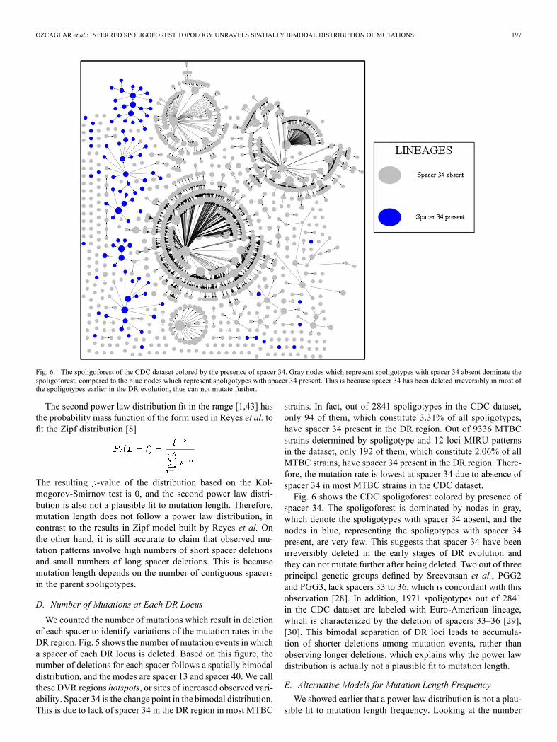
Fig. 6. The spoligoforest of the CDC dataset colored by the presence of spacer 34. Gray nodes which represent spoligotypes with spacer 34 absent dominate thespoligoforest, compared to the blue nodes which represent spoligotypes with spacer 34 present. This is because spacer 34 has been deleted irreversibly in most ofthe spoligotypes earlier in the DR evolution, thus can not mutate further.

The second power law distribution fit in the range [1,43] hasthe probability mass function of the form used in Reyes et al. tofit the Zipf distribution [8]

The resulting -value of the distribution based on the Kol-mogorov-Smirnov test is 0, and the second power law distri-bution is also not a plausible fit to mutation length. Therefore,mutation length does not follow a power law distribution, incontrast to the results in Zipf model built by Reyes et al. Onthe other hand, it is still accurate to claim that observed mu-tation patterns involve high numbers of short spacer deletionsand small numbers of long spacer deletions. This is becausemutation length depends on the number of contiguous spacersin the parent spoligotypes.

D. Number of Mutations at Each DR Locus

We counted the number of mutations which result in deletionof each spacer to identify variations of the mutation rates in theDR region. Fig. 5 shows the number of mutation events in whicha spacer of each DR locus is deleted. Based on this figure, thenumber of deletions for each spacer follows a spatially bimodaldistribution, and the modes are spacer 13 and spacer 40. We callthese DVR regions hotspots, or sites of increased observed vari-ability. Spacer 34 is the change point in the bimodal distribution.This is due to lack of spacer 34 in the DR region in most MTBC

strains. In fact, out of 2841 spoligotypes in the CDC dataset,only 94 of them, which constitute 3.31% of all spoligotypes,have spacer 34 present in the DR region. Out of 9336 MTBCstrains determined by spoligotype and 12-loci MIRU patternsin the dataset, only 192 of them, which constitute 2.06% of allMTBC strains, have spacer 34 present in the DR region. There-fore, the mutation rate is lowest at spacer 34 due to absence ofspacer 34 in most MTBC strains in the CDC dataset.Fig. 6 shows the CDC spoligoforest colored by presence of

spacer 34. The spoligoforest is dominated by nodes in gray,which denote the spoligotypes with spacer 34 absent, and thenodes in blue, representing the spoligotypes with spacer 34present, are very few. This suggests that spacer 34 have beenirreversibly deleted in the early stages of DR evolution andthey can not mutate further after being deleted. Two out of threeprincipal genetic groups defined by Sreevatsan et al., PGG2and PGG3, lack spacers 33 to 36, which is concordant with thisobservation [28]. In addition, 1971 spoligotypes out of 2841in the CDC dataset are labeled with Euro-American lineage,which is characterized by the deletion of spacers 33–36 [29],[30]. This bimodal separation of DR loci leads to accumula-tion of shorter deletions among mutation events, rather thanobserving longer deletions, which explains why the power lawdistribution is actually not a plausible fit to mutation length.

E. Alternative Models for Mutation Length Frequency

We showed earlier that a power law distribution is not a plau-sible fit to mutation length frequency. Looking at the number


TABLE IIIPOSSIBLE START AND END POINT REGIONS OF MUTATION EVENTS. THE TABLESHOWS THAT A MUTATION EVENT CAN START AND END EITHER IN REGION1 INCLUDING SPACERS [1,34], LEADING TO TYPE I MUTATION EVENT, OR ITCAN START AND END IN REGION 2 INCLUDING SPACERS [35,43], LEADING

TO TYPE II MUTATION EVENT

of mutations at each spacer shown in Fig. 5, we can see thatthe mutation length depends on the starting point of the muta-tion. Based on this observation, we built two alternative modelsfor mutation length frequency: Starting Point Model (SPM) andLongest Block Model (LBM). SPM conditions the mutationlength on the starting point of the mutation, and fits power lawdistributions to mutation length frequency. LBM conditions themutation length on the length of longest block of 1’s, or presentspacers, beyond the starting point of mutation on each mutatedspoligotype. In this section, we describe both models in detailand show that they are plausibly good fits to mutation lengthfrequency.1) Starting Point Model (SPM): The number of mutations

follows a spatially bimodal distribution as shown in Fig. 5, andspacer 34 is the change point of this distribution with the fewestnumber of mutations. We relax this assumption and separate thespacers into two regions: region 1 including spacers [1,34], andregion 2 including spacers [35,43]. Without loss of generality,we assume that a mutation event starts at a lower-indexed spacerand ends at a higher-indexed spacer. Table III shows all start andend point combinations of mutation events, and whether theyare possible or not. According to the table, both start and endpoints of a mutation event have to be in the same spacer region,either in [1,34], or in [35,43]. Therefore, no mutation event canresult in deletion of spacers in both regions. We name mutationevents which start and end at region 1 in the range [1,34] asType I mutation event, and mutation events which start and endat region 2 in the range [35,43] as Type II mutation event.

(1)

Let variable represent the mutation length, and variablerepresent the starting point of mutation. Fig. 7 shows the numberof mutations of length which start at spacer . No-tice that, at each starting point except spacers 34 and 43, themutation length frequency follows a power law distribution, asverified by goodness-of-fit test. Using maximum likelihood es-timation, we verified that the mutation length frequency followsa power law distribution with a unique power law exponent foreach starting point . At the boundarystarting spacers 34 and 43, since the mutation event can occur

Fig. 7. The number of mutations of length which start at spacer .For each starting point except 34 and 43, mutation length frequency follows apower law distribution, as verified by a goodness-of-fit test. For starting points34 and 43, the only possible mutation length is 1.

in one of the two regions, the only possible mutation length is1. These observations lead to the SPM described in (1), whereis the exponent of power law distribution for starting point .

The values are estimated from the CDC data using maximumlikelihood method to compute the values. Inorder to find the mutation length distribution, valuesare calculated as follows:

(2)

where is calculated as follows. For each spoligo-type in the dataset, present spacers are found and added to thetotal count for each spacer. Then, is the ratio of thenumber of spoligotypes with spacer present to the total numberof spacers present in all spoligotypes. Note thatvalues are derived from the spoligotype signatures of strains,without the need to find the mutation history of spoligotypesusing MakeSpoligoforest() algorithm.Given values calculated using (2), Fig. 8 shows

the cumulative distribution for the SPM on a log-logplot. In order to test the goodness-of-fit of SPM, we adapted thepower law validation procedure by Clauset et al. to this model.Table IV shows that the -value for SPM is 1, which is greaterthan 0.1, which suggests that SPM is a plausible model for themutation length frequency distribution.2) Longest Block Model (LBM): According to the con-

tiguous deletion assumption, a block of contiguous spacers canbe deleted in a mutation event. Therefore, given the startingpoint of a mutation on a spoligotype, the number of spacersthat can be deleted is limited by the number of contiguousspacers beyond the starting point. Let represent the mutationlength, and let be the upper bound on the mutation length,given the starting point of the mutation on a spoligotype. Fig. 9shows a spoligotype with present spacers in gray, and absentspacers in white. If the starting point of mutation is , then the


Fig. 8. Cumulative distribution of SPM based on the CDC dataset.SPM is a good model for mutation length frequency distribution. The good-ness-of-fit test returns a -value of 1, which verifies the accuracy of the model.

TABLE IVCANDIDATE MODELS FOR MUTATION LENGTH FREQUENCY DISTRIBUTION ANDTHEIR GOODNESS-OF-FIT TEST RESULTS BASED ON KOLMOGOROV-SMIRNOVTEST. THE -VALUE FOR BOTH SPM AND LBM IS 1, WHICH SUGGESTS THATBOTH MODELS ESTIMATE THE MUTATION LENGTH FREQUENCY DISTRIBUTION

ACCURATELY

Fig. 9. Given the starting point of mutation on a spoligotype, the contiguousblock of spacers beyond the starting point can be deleted in a mutation event. Inthe example above, given that the mutation starts at spacer , the length of themutation can be at most .

mutation length can be at most . Based on this observation,in Fig. 10, we plotted the number of mutations of length ,given the maximum possible length . In the plot, at each

value except , the mutation length frequencyfollows a power law distribution if , alsoverified by goodness-of-fit test. We verified using maximumlikelihood estimation that the mutation length frequencyfollows a power law distribution with a unique power lawexponent for each , given that . Atthe boundary case , the mutation can only be of length1. These observations are combined in the LBM described in(3),

(3)

Fig. 10. The number of mutations of length , given that the longest blockof contiguous spacers is of length . If there exists at least one blockof contiguous spacers of length , then, given the upper bound ,the mutation length frequency follows power law distribution.

Fig. 11. Cumulative distribution of LBM based on the CDC dataset.LBM is a good model for mutation length frequency distribution. The good-ness-of-fit test returns a -value of 1, which verifies the accuracy of the model.

where is the exponent of power law distribution formaximum length . The values are estimatedfrom the CDC data using maximum likelihood method, and

values are found. Mutation length distri-bution is derived from this probability as follows:

(4)

where values are calculated from the mutationhistory of spoligotypes using starting point of eachmutation andthereby the length of the longest block of contiguous spacers foreach mutation event.Given values calculated using (4), Fig. 11 shows

the cumulative distribution for LBM on a log-log


Fig. 12. Cumulative distribution for SPM and LBM based on the Institut Pasteur de Guadeloupe dataset. SPM and LBM fits the mutation lengthfrequency distribution. This shows that these models are robust and they hold for different strain datasets. (a) SPM. (b) LBM.

TABLE VGOODNESS-OF-FIT TEST RESULTS OF SPM AND LBM FOR THE DATASET FROMINSTITUT PASTEUR DE GUADELOUPE, BASED ON KOLMOGOROV-SMIRNOVTEST. THE -VALUE FOR SPM AND LBM IS 1, WHICH SUGGESTS THAT BOTHMODELS ESTIMATE THE MUTATION LENGTH FREQUENCY DISTRIBUTIONACCURATELY. THIS SHOWS THAT SPM AND LBM ARE ROBUST AND THEY

HOLD FOR DIFFERENT STRAIN DATASETS

plot. We tested the goodness-of-fit of LBM using the test weadapted from power law validation procedure by Clauset et al.As shown in Table IV, the -value of the test for LBM is 1,which is greater than 0.1. This suggests that LBM is a plausiblemodel for the mutation length frequency distribution.In both SPM and LBM, we used an extra parameter to es-

timate the mutation length frequency distribution. To test if themodels are robust, we applied SPM and LBM to another datasetfrom Institut Pasteur de Guadeloupe which is partially listed inmultimarker SITVITWEB database [31]. This dataset has 2158strains uniquely identified by (spoligotype, MIRU) pairs, andthere are 699 unique spoligotypes.We ran the MakeSpoligo-forest() algorithm on this dataset, and fit SPM and LBM tothe mutation length frequency distribution. Fig. 12(a) and 12(b)shows the cumulative distribution for SPM and LBMrespectively. The goodness-of-fit test results for both models aresummarized in Table V. The -value for both models is 1, whichis greater than 0.1, and this suggests that SPM and LBM areplausibly good models for the mutation length frequency distri-bution. Therefore, SPM and LBM are robust and they accuratelyestimate the mutation length frequency distribution independentof the dataset examined.

V. DISCUSSION AND CONCLUSION

We developed a new mutation model of MTBC spoligotypeevolution using the variations in the DR region and MIRU

patterns to disambiguate the ancestors of a spoligotype. Basedon the contiguous deletion assumption and no homoplasy, andusing three distance measures, we generated the most parsimo-nious forest of spoligotypes. The resulting spoligoforest depictsa putative history of mutation events in the DR region. Giventhe spoligotype mutations, we analyzed the biological networkof spoligotypes in terms of both network topology and numberof mutations at each DR locus.We compared our mutation model based on spoligotypes and

MIRU patterns with its counterparts using spoligotyping only,MIRU typing only and with Zipf model [8]. The mutation modelwhich incorporates both biomarkers results in the most par-simonious spoligoforest and maximizes within-lineage muta-tion events. The comparison showed that segregation accuracyvalues are high in all four models with no statistically signif-icant difference in the results. Therefore, spoligoforests cre-ated using only spoligotypes and the Zipf model are very sim-ilar to spoligoforests determined by the additional independentbiomarker MIRU-VNTR. This validates the spoligoforest algo-rithms based only on spoligotypes, showing that spoligotypeonly algorithms can be used to generate the spoligoforest whenMIRU patterns are not present.The number of descendants of a spoligotype is equivalent to

the outdegree of the corresponding node in the spoligoforest.Wetested and verified the hypothesis that the number of descendantspoligotypes follows a power law distribution. This is due to thefact that the higher the copy number of spoligotype, that is, themore spacers present in the DR region, the more spoligotypescan descend from it. In addition, the assumption of no homo-plasy favors genetic diversity rather than convergent evolution.We tested and verified that mutation length of spoligotype

deletions in a mutation event does not follow a power law dis-tribution, as opposed to the Zipf model for mutation of spoligo-types proposed by Reyes et al. [8]. However, it is still accurateto state that mutations in the DR region rarely involve long dele-tions and frequently involve short deletions.


We calculated the number of mutation events which resultedin deletion of spacer at each DR locus. The number of muta-tions at consecutive DR loci showed a pattern of spatially bi-modal distribution. The two modes are spacer 13 and spacer 40,which are hotspots of variations in the DR region. The changepoint in the bimodal distribution is spacer 34. This is due to ab-sence of spacer 34 in a large number of MTBC strains, ratherthan low mutation rate at DVR34, because this spacer has beendeleted irreversibly at the beginning of DR evolution and it cannot mutate further after being deleted. Two out of three prin-cipal genetic groups defined by Sreevatsan et al. and MTBCstrains of Euro-American lineage lack spacers 33–36, whichsupports the claim that low number of mutations in DVR34is due to lack of spacer 34 in most MTBC strains in the CDCdataset [28], [29]. Since most of the deletion events occur eitheron spacers 1–34, or spacers 35–43, resulting in accumulationof shorter deletions, longer deletions are not observed. There-fore, this bimodal distribution explains why mutation lengthdoes not follow a power law distribution. Note however thata block of contiguous spacers in the 43-spacer format may notbe contiguous in the 104-spacer format, which is a superset of43-spacer format [32]. Therefore, 43-spacer representation canbe renumbered on the 104-spacer format for further differentia-tion of spoligotypes to build a more detailed mutation history ofthe DR region. Spacer duplications can also intervene a blockof contiguous spacers during the microevolution of geneticallyrelated group of strains, and a deletion involving a duplicatedspacer can not be captured by the 43-spacer format [33].Based on the spatially bimodal distribution of mutation

events in the DR region, we built two alternative models formutation length frequency. The SPM conditions the mutationlength on the starting point of the mutation, and the LBM con-ditions the mutation length on the length of the longest blockof contiguous spacers beyond the starting point of mutation.Both SPM and LBM estimate the mutation length frequencydistribution accurately, as opposed to Zipf model suggested inearlier studies. We also tested these models on another datasetfrom Institut Pasteur de Guadeloupe, and verified that bothmodels are robust and hold for different strain datasets.Future work will involve analysis of other topological

attributes of the spoligoforest, extension of the mutationmodel to use other biomarkers, and interpretation of cladesgrouped closely in the spoligoforest. The mutation model canbe extended to include more biomarkers, e.g., RFLP, withcorresponding distance measures for the additional biomarkersto be used in the algorithm which generates the spoligoforest.Analysis of connected components in the spoligoforest can givemore insight into segregation of major lineages or sublineages.In addition, each tree or subtree in the spoligoforest can bea group of genetically related MTBC strains not classifiedas a separate clade earlier. This mutation model can also beextended to other organisms genotyped by CRISPR profiles.

ACKNOWLEDGMENT

This work was made possible by Dr. Lauren Cowan and Dr.Jeff Driscoll of the Centers for Disease Control and Prevention.The authors thank Dr. Aaron Clauset and Dr. Cosma Shalizi for

providing the implementations of the methods to fit power lawdistributions.

REFERENCES

[1] “Global tuberculosis control: Epidemiology, strategy, financing,”World Health Organization, Geneva, Switzerland, WHO Rep., 2009.

[2] A. Shabbeer, C. Ozcaglar, B. Yener, and K. P. Bennett, “Web tools formolecular epidemiology of tuberculosis,” Infection, Genet., Evol., vol.12, no. 4, pp. 767–781, 2012.

[3] B. Mathema, N. E. Kurepina, P. J. Bifani, and B. N. Kreiswirth,“Molecular epidemiology of tuberculosis: Current insights,” Clin.Microbiol. Rev., vol. 19, no. 4, pp. 658–685, 2006.

[4] C. Ozcaglar, A. Shabbeer, S. Vandenberg, B. Yener, and K. P. Bennett,“Sublineage structure analysis of Mycobacterium tuberculosis com-plex strains using multiple-biomarker tensors,” BMC Genomics, vol.12, p. S1, 2011, no. Suppl 2.

[5] R. Brosch, S. V. Gordon, M. Marmiesse, P. Brodin, C. Buchrieser, K.Eiglmeier, T. Garnier, C. Gutierrez, G. Hewinson, K. Kremer, L. M.Parsons, A. S. Pym, S. Samper, D. van Soolingen, and S. T. Cole, “Anew evolutionary scenario for the Mycobacterium tuberculosis com-plex,” PNAS, vol. 99, no. 6, pp. 3684–3689, 2002.

[6] S. T. Cole, R. Brosch, J. Parkhill, T. Garnier, C. Churcher, D. Harris, S.V. Gordon, K. Eiglmeier, S. Gas, C. E. Barry, F. Tekaia, K. Badcock, D.Basham, D. Brown, T. Chillingworth, R. Connor, R. Davies, K. Devlin,T. Feltwell, S. Gentles, N. Hamlin, S. Holroyd, T. Hornsby, K. Jagels,A. Krogh, J. McLean, S. Moule, L. Murphy, K. Oliver, J. Osborne, M.A. Quail, M. A. Rajandream, J. Rogers, S. Rutter, K. Seeger, J. Skelton,R. Squares, S. Squares, J. E. Sulston, K. Taylor, S. Whitehead, and B.G. Barrell, “Deciphering the biology of Mycobacterium tuberculosisfrom the complete genome sequence,” Nature, vol. 393, pp. 537–544,Jun. 1998.

[7] M. M. Tanaka and A. R. Francis, “Methods of quantifying and visual-ising outbreaks of tuberculosis using genotypic information,” Infection,Genet., Evol., vol. 5, pp. 35–43, 2005.

[8] J. Reyes, A. Francis, and M. Tanaka, “Models of deletion for visual-izing bacterial variation: An application to tuberculosis spoligotypes,”BMC Bioinformatics, vol. 9, no. 1, p. 496, 2008.

[9] A. Grant, C. Arnold, N. Thorne, S. Gharbia, andA. Underwood, “Math-ematical modelling of Mycobacterium tuberculosis VNTR loci esti-mates a very slow mutation rate for the repeats,” J. Mol. Evol., vol.66, pp. 565–574, 2008.

[10] E. R. Gansner and S. C. North, “An open graph visualization systemand its applications to software engineering,” Softw. Pract. Exper., vol.30, no. 11, pp. 1203–1233, 2000.

[11] J. F. Reyes andM.M. Tanaka, “Mutation rates of spoligotypes and vari-able numbers of tandem repeat loci in Mycobacterium tuberculosis,”Infection, Genet., Evol., vol. 10, no. 7, pp. 1046–1051, 2010.

[12] J. D. A. van Embden, T. van Gorkom, K. Kremer, R. Jansen, B. A. M.van der Zeijst, and L. M. Schouls, “Genetic variation and evolutionaryorigin of the direct repeat locus of Mycobacterium tuberculosis com-plex bacteria,” J. Bacteriol., vol. 182, no. 9, pp. 2393–2401, 2000.

[13] R. M. Warren, E. M. Streicher, S. L. Sampson, G. D. van der Spuy,M. Richardson, D. Nguyen, M. A. Behr, T. C. Victor, and P. D. vanHelden, “Microevolution of the direct repeat region ofMycobacteriumtuberculosis: Implications for interpretation of spoligotyping data,” J.Clin. Microbiol., vol. 40, no. 12, pp. 4457–4465, 2002.

[14] J. Zhang, E. Abadia, G. Refregier, S. Tafaj, M. L. Boschiroli, B. Guil-lard, A. Andremont, R. Ruimy, and C. Sola, “Mycobacterium tubercu-losis complex CRISPR genotyping: Improving efficiency, throughputand discriminative power of ‘spoligotyping’ with new spacers and amicrobead-based hybridization assay,” J. Med. Microbiol., vol. 59, no.3, pp. 285–294, 2010.

[15] J. Kamerbeek, L. Schouls, A. Kolk, M. van Agterveld, D. vanSoolingen, S. Kuijper, A. Bunschoten, H. Molhuizen, R. Shaw,M. Goyal, and J. van Embden, “Simultaneous detection and straindifferentiation of Mycobacterium tuberculosis for diagnosis andepidemiology,” J. Clin. Microbiol., vol. 35, no. 4, pp. 907–914, 1997.

[16] P. Supply, J. Magdalena, S. Himpens, and C. Locht, “Identificationof novel intergenic repetitive units in a mycobacterial two-componentsystem operon,” Mol. Microbiol., vol. 26, no. 5, pp. 991–1003, 1997.

[17] P. Supply, E. Mazars, S. Lesjean, V. Vincent, B. Gicquel, and C. Locht,“Variable human minisatellite-like regions in the Mycobacterium tu-berculosis genome,”Mol.Microbiol., vol. 36, no. 3, pp. 762–771, 2000.


[18] P. Supply, C. Allix, S. Lesjean, M. Cardoso-Oelemann, S.Rusch-Gerdes, E. Willery, E. Savine, P. de Haas, H. van Deutekom, S.Roring, P. Bifani, N. Kurepina, B. Kreiswirth, C. Sola, N. Rastogi, V.Vatin, M. C. Gutierrez, M. Fauville, S. Niemann, R. Skuce, K. Kremer,C. Locht, and D. van Soolingen, “Proposal for standardization ofoptimized mycobacterial interspersed repetitive unit-variable-numbertandem repeat typing of Mycobacterium tuberculosis,” J. Clin. Micro-biol., vol. 44, pp. 4498–4510, Dec. 2006.

[19] J. Camin and R. Sokal, “A method for deducting branching sequencesin phylogeny,” Evolution, vol. 19, pp. 311–326, 1965.

[20] J. Felsenstein, Inferring Phylogenies. Sunderland, MA: Sinauer,2003.

[21] M. Kimura and T. Ohta, “Stepwise mutation model and distributionof allelic frequencies in a finite population,” PNAS, vol. 75, pp.2868–2872, June 1978.

[22] T. Wirth, F. Hildebrand, C. Allix-Béguec, F. Wölbeling, T. Kubica, K.Kremer, D. van Soolingen, S. Rüsch-Gerdes, C. Locht, S. Brisse, A.Meyer, P. Supply, and S. Niemann, “Origin, spread and demographyof the Mycobacterium tuberculosis complex,” PLoS Pathogen, vol. 4,p. e1000160, Sep. 2008.

[23] M. Aminian, A. Shabbeer, and K. P. Bennett, “A conformal Bayesiannetwork for classification ofMycobacterium tuberculosis complex lin-eages,” BMC Bioinformatics, vol. 11, p. S4, 2010, no. Suppl 3.

[24] G. Pavlopoulos, M. Secrier, C. Moschopoulos, T. Soldatos, S. Kossida,J. Aerts, R. Schneider, and P. Bagos, “Using graph theory to analyzebiological networks,” BioData Mining, vol. 4, no. 1, p. 10+, 2011.

[25] G. Lima-Mendez and J. Helden, “The powerful law of the power lawand other myths in network biology,” Mol. BioSyst., vol. 5, no. 12, pp.1482–1493, 2009.

[26] A. Clauset, C. R. Shalizi, and M. E. J. Newman, “Power-law distribu-tions in empirical data,” SIAM Rev., vol. 51, p. 661+, Feb. 2009.

[27] C. Tang, J. Reyes, F. Luciani, A. R. Francis, and M. M. Tanaka,“spolTools: Online utilities for analyzing spoligotypes of the My-cobacterium tuberculosis complex,” Bioinformatics, vol. 24, no. 20,pp. 2414–2415, 2008.

[28] S. Sreevatsan, X. Pan, K. E. Stockbauer, N. D. Connell, B. N.Kreiswirth, T. S. Whittam, and J. M. Musser, “Restricted structuralgene polymorphism in the Mycobacterium tuberculosis complexindicates evolutionarily recent global dissemination,” PNAS, vol. 94,no. 18, pp. 9869–9874, 1997.

[29] S. Gagneux, K. DeRiemer, T. Van, M. Kato-Maeda, B. C. de Jong, S.Narayanan, M. Nicol, S. Niemann, K. Kremer, M. C. Gutierrez, M.Hilty, P. C. Hopewell, and P. M. Small, “Variable host-pathogen com-patibility in Mycobacterium tuberculosis,” PNAS, vol. 103, no. 8, pp.2869–2873, 2006.

[30] C. Borile, M. Labarre, S. Franz, C. Sola, and G. Refregier, “Usingaffinity propagation for identifying subspecies among clonal organ-isms: Lessons fromM. tuberculosis,” BMC Bioinformatics, vol. 12, no.1, p. 224, 2011.

[31] C. Demay, B. Liens, T. Burguiére, V. Hill, D. Couvin, J. Millet, I.Mokrousov, C. Sola, T. Zozio, and N. Rastogi, “SITVITWEB—Apublicly available international multimarker database for studyingMycobacterium tuberculosis genetic diversity and molecular epidemi-ology,” Infection, Genet., Evol., vol. 12, no. 4, pp. 755–766, 2012.

[32] A. G. M. van der Zanden, K. Kremer, L. M. Schouls, K. Caimi, A.Cataldi, A. Hulleman, N. J. D. Nagelkerke, and D. van Soolingen,“Improvement of differentiation and interpretability of spoligotypingfor Mycobacterium tuberculosis complex isolates by introduction ofnew spacer oligonucleotides,” J. Clin. Microbiol., vol. 40, no. 12, pp.4628–4639, 2002.

[33] B. Mathema, N. Kurepina, G. Yang, E. Shashkina, C. Manca, C.Mehaffy, H. Bielefeldt-Ohmann, S. Ahuja, D. A. Fallows, A. Izzo, P.Bifani, K. Dobos, G. Kaplan, and B. N. Kreiswirth, “Epidemiologicconsequences of microvariation in Mycobacterium tuberculosis,” J.Infectious Diseases, vol. 205, no. 6, pp. 964–974, 2012.

Authors’ photographs and biographies not available at the time of publication.

ieee transactions on nanobioscience, vol. 11, no. 3...

Documents