ieee transactions on robotics 1 cooperative …web.mit.edu/nsl/www/preprints/robot_sync_09.pdf ·...

IEEE TRANSACTIONS ON ROBOTICS 1

Cooperative Robot Control and ConcurrentSynchronization of Lagrangian Systems

Soon-Jo Chung, Member, IEEE, and Jean-Jacques Slotine

Abstract

Concurrent synchronization is a regime where diverse groups of fully synchronized dynamic systems stably coexist. We studyglobal exponential synchronization and concurrent synchronization in the context of Lagrangian systems control. In a networkconstructed by adding diffusive couplings to robot manipulators or mobile robots, a decentralized tracking control law globallyexponentially synchronizes an arbitrary number of robots, and represents a generalization of the average consensus problem. Exactnonlinear stability guarantees and synchronization conditions are derived by contraction analysis. The proposed decentralizedstrategy is further extended to adaptive synchronization and partial-state coupling.

I. INTRODUCTION

Distributed and decentralized synchronization of large groups of dynamic systems is an area of intensive research. Inthis article, we study cooperative control and global exponential synchronization of groups of Lagrangian systems, such asmechanical robots. Our results apply both to exact matching of all individual state variables, or, through a translation of thestate space, to convergence to specific (perhaps time-varying) formation patterns. Furthermore, we construct complex robotnetworks where multiple groups of fully synchronized elements coexist. Such concurrent synchronization seems pervasive inbiology, and in particular in the brain where multiple rhythms coexist and neurons can exhibit many qualitatively differenttypes of oscillations [34].

The objective of this paper is to establish a unified synchronization framework that can achieve both synchronization of theconfiguration variables of the robots and stable tracking of a common desired trajectory. Although an uncoupled trajectorytracking control law, in the absence of external disturbances, would achieve synchronization to a common desired trajectory,the presence of various disturbances motivates the mutual synchronization of the system variables. On the other hand, thesynchronization to the average of initial conditions is not sufficient for multi-robot or multi-vehicle systems where a desiredtrajectory is explicitly given. For example, a large swarm of robots can first synchronize their attitudes and positions to form acertain formation pattern, then track the common desired trajectory to accomplish the given mission. In production processes,such as manufacturing and automotive applications, where high flexibility, manipulability, and maneuverability cannot beachieved by a single system [38], there has been widespread interest in cooperative schemes for multiple robot manipulatorsthat track a predefined trajectory. A stellar formation flight interferometer [8], [9] is another example where precision controlof relative spacecraft motions is indispensable. The proposed synchronization tracking control law can be implemented forsuch purposes, where a common desired trajectory can be explicitly given. The proposed strategy can achieve more efficientand robust performance through local interactions, especially in the presence of non-identical external disturbances. Further,we generalize the proposed control law such that multiple dynamic systems can synchronize themselves from arbitrary initialconditions without the need for a common reference trajectory. As a result, other potential applications include oscillationsynchronization of robotic locomotion [15], [35], [39], and tele-manipulation of robots [3], [29].

The main contributions of this work can be stated as follows.• Concurrent synchronization that exploits the multiple time scale behaviors from two types of inputs (a reference trajectory

and local couplings) permits construction of a complex time-varying network comprised of numerous heterogeneoussystems.

• In contrast with prior work on consensus and flocking problems using graphs, the proposed strategy primarily deals withdynamic networks consisting of nonlinear time-varying dynamics.

• We use contraction analysis [26], [47] as our main nonlinear stability tool, thereby deriving exact and global results withexponential convergence, as opposed to asymptotic convergence of prior work.

• The proposed control laws are of a decentralized form requiring only local velocity/position coupling feedback for globalexponential convergence, thereby facilitating implementation in real systems.

• The theory is generalized and extended to multi-robot systems with non-identical dynamics, linear coupling control, partialstate coupling, uni-directional coupling, and adaptive control.

Assistant Professor of Aerospace Engineering, Iowa State University, Ames, IA 50011, E-mail: [email protected] of Mechanical Engineering & Information Sciences, Professor of Brain & Cognitive Sciences, Massachusetts Institute of Technology, Cambridge,

MA 02319, E-mail: [email protected].


A. Comparison with Related Work

The consensus problems on graph [30] and the coordination of multi-agent systems [17], [25], [31], [32] are closely relatedwith the synchronization problem. In particular, the use of graph theory and Laplacian produced many interesting results [17],[22], [25], [28], [30], [36], [37]. However, the synchronization to the average of initial conditions might not be directly applicableto multi-robot and multi-vehicle systems, where a desired trajectory is explicitly defined. A recent work [36] studied theconsensus problem with a time-varying reference state, based on a single integrator model. In essence, the aforementioned workmainly deals with simple dynamic models such as linear systems and single or double integrator models without nonlinearlycoupled inertia matrices. In contrast, we aim at addressing highly nonlinear systems (e.g. helicopters, attitude dynamics ofspacecraft, walking robots, and manipulator robots). As shall be seen later, the proof of the synchronization for network systemsthat possess nonlinearly coupled inertia matrices is more involved. This paper focuses on such dynamic networks consistingof highly nonlinear systems.

One notable work [38] introduced a nonlinear tracking control law that synchronized multiple robot manipulators in order totrack a common desired trajectory. Due to its all-to-all coupling requirement, the number of variables to be estimated increaseswith the number of robots to be synchronized, which imposes a significant communication burden. Additionally, the feedbackof estimated acceleration errors requires unnecessary information and complexity. Thus, a method to eliminate both the all-to-allcoupling and the feedback of the acceleration terms is explored in this paper. Another nice approach to the synchronizationof robot networks is to exploit the passivity of the input-output dynamics [3], [4]. Its property of robustness to time delays isparticularly attractive, while robot dynamics are passive only with velocity outputs unless composite variables are employed. Inaddition, the mutual synchronization problem, which not only synchronizes the sub-members but also enforces them to followa common reference trajectory, is not addressed. In particular, it shall be shown that our proposed control law generalizesthe robot control law presented in [4], while our convergence result is stronger (exponential). One recent work [16] usedthe passivity property for the path-following system to synchronize the path variables. The passive decomposition [21], [22]describes a strategy of decoupling into the internal group formation shape and the total group maneuver. Due to its dependencyon a centralized control architecture, the decoupling is not generally ensured under the decentralized control. [22] considerslinear double integrator models. Another work [12] proposed a nice control framework for controlling and coordinating agroup of nonholonomic mobile robots, although the exact synchronization of individual vehicles was not pursued. One recentwork [33] presented a framework called particles with coupled oscillator dynamics so that collective spatial patterns emerge.Our recent work [9] also discussed more complex spacecraft dynamics to achieve the phase synchronization of spiral or circulartranslational trajectories in three dimensions as well as the synchronization of rotational dynamics. Also, it is important to notethat the adaptive synchronization of multiple robotic manipulators in a single local coupling configuration was studied in [45],[46].

The proposed synchronization framework using contraction analysis, first reported in [6], has a clear advantage in its broadapplications to a larger class of identical or nonidentical nonlinear systems even with complex coupling geometry includinguni-directional couplings and partial degrees-of-freedom couplings, non-passive input-output, and time delays [7], [48], whileensuring a simple decentralized coupling control law (see Figure 1 for network structures permitted here). The proofs and newresults from [6] are expanded in this paper. In particular, concurrent synchronization that exploits two different types of inputshas not been studied in the literature.

B. Organization

Section II describes modeling of robots based on the Lagrangian formulation, and summarizes the key stability theorems.While Section III presents the main control law and its tracking stability, the proof of exponential synchronization is moreinvolved and treated separately in Section IV. The remainder of the paper further highlights the unique contributions of thiswork. Section V elucidates the concurrent synchronization of complex networks and the leader-follower problem. The mainidea of this paper is extended to linear Proportional-Derivative (PD) couplings, and limited partial-state couplings in SectionVI. Key simulation results are also presented in Section VI.

II. MODELING AND NONLINEAR STABILITY TOOLS FOR MULTI-ROBOT NETWORKS

A. Lagrangian Systems

This paper is devoted to the use of the Lagrangian formulation for its simplicity in dealing with complex systems involvingmultiple dynamics. The equations of motion for a robot with multiple joints (qi ∈ Rn) can be derived by exploiting theEuler-Lagrange equations:

Li =12qT

i Mi(qi)qi − Vi,d

dt

∂Li(qi, qi)∂qi

− ∂Li(qi, qi)∂qi

= τi (1)

where i, (1 ≤ i ≤ p) denotes the index of robots or dynamic systems comprising a network, and p is the total number of theindividual elements. Equation (1) can be represented as

Mi(qi)qi + Ci(qi, qi)qi + gi(qi) = τi (2)


where gi(qi) = ∂Vi

qi, and, τi is a generalized force or torque acting on the i-th robot.

Note that we define Ci(qi, qi) such that (Mi − 2Ci) is skew-symmetric [40], and this property plays a central role in ourstability analysis using contraction theory [7].

The following key assumptions are used throughout this paper. Since the main applications of the present paper includefully actuated robot manipulators and spacecraft [9], the robot system in (2) is fully actuated. In other words, the number ofcontrol inputs is equal to the dimension of their configuration manifold (= n). The mass-inertia matrix M(q) is assumed tobe uniformly positive definite, for all positions q in the robot workspace [40].

B. Contraction Analysis for Global and Exponential Stability

(1) Modular Stability Analysis: Although one popular method for modular stability analysis is to exploit the passivity for-malism [40], we use contraction theory [26], [34], [41], [47] as an alternative tool for analyzing modular stability of couplednonlinear systems. In particular, contraction analysis has more general and intuitive combination properties (e.g., hierarchies)than the passivity method, since it involves a state-space rather than an input-output method.(2) Differential State-State Analysis: Lyapunov’s linearization method indicates that the local stability of the nonlinear systemcan be analyzed using its differential approximation. What is new in contraction theory is that a differential stability analysiscan be made exact, thereby yielding global results on the time-varying nonlinear system.(3) Stronger Stability Results (Exponential and Global): For a robot dynamic model in (2) and a time-varying tracking controllaw, the straightforward use of Barbalat’s lemma or LaSalle-Yoshizawa theorem [20] yields asymptotic convergence results.While global exponential stability can be proven by using a Lyapunov function with a cross-term and additional constraints [1],[2], [19], such a method is ad hoc, as compared to contraction theory. While exact exponential convergence might not beachievable in real systems due to the modeling errors, we believe that finding an explicit convergence rate with exponentialstability, if possible, is important due to its superior tracking performance and property of robustness with respect to perturbations(e.g., see p. 339–350 in [19]).

A brief review of the results from [26], [41], [47] is presented in this section. Note that contraction theory is a generalizationof the classical Krasovskii’s theorem [40], and that approaches closely related to contraction, although not based on differentialanalysis, can be traced back to [10], [11], [14] and even to [24].

Consider a smooth nonlinear systemx(t) = f(x(t),u(x, t), t) (3)

where x(t) ∈ Rn, and f : Rn × Rm × R+ → Rn. A virtual displacement, δx is defined as an infinitesimal displacement at afixed time– a common supposition in the calculus of variations.

Theorem 1: For the system in (3), if there exists a uniformly positive definite metric,

M(x, t) = Θ(x, t)T Θ(x, t) (4)

where Θ is some smooth coordinate transformation of the virtual displacement, δz = Θδx, such that the associated generalizedJacobian, F is uniformly negative definite, i.e., ∃λ > 0 such that

F =(

Θ(x, t) + Θ(x, t)∂f∂x

)Θ(x, t)−1 ≤ −λI, (5)

then all system trajectories converge globally to a single trajectory exponentially fast regardless of the initial conditions, witha global exponential convergence rate of the largest eigenvalues of the symmetric part of F.Such a system is said to be contracting. The proof is given in [26]. Equivalently, the system is contracting if ∃λ > 0 such that

M +(∂f∂x

)T

M + M∂f∂x≤ −2λM (6)

Equation (6) is useful for the stability proof of a Lagrangian system, since the inertia matrix M(q) of the robot dynamics in(2) can be chosen as the metric M in (6).

The key advantage of contraction analysis is its superior combination property as follows.

C. Contraction of Coupled Systems

The following theorems are used to derive stability and synchronization of coupled Lagrangian systems.Theorem 2: Hierarchical combination [41]. Consider two contracting systems, of possibly different dimensions and metrics,

and connect them in series, leading to a smooth virtual dynamics of the form

d

dt

(δz1

δz2

)=(

F11 0F21 F22

)(δz1

δz2

)Then, the combined system is contracting if F21 is bounded.


Proof: see [7], [41], [42].Theorem 3: Partial contraction [47]. Consider a nonlinear system of the form x = f(x,x, t) and assume that the auxiliary

system y = f(y,x, t) is contracting with respect to y. If a particular solution of the auxiliary y-system verifies a specificsmooth property, then all trajectories of the original x-system verify this property exponentially. The original system is said tobe partially contracting.

Proof: See [47] for the virtual observer-like y system.Theorem 4: Synchronization [47]. Consider two coupled systems. If the dynamics equations verify

x1 − f(x1, t) = x2 − f(x2, t)

where the function f(x, t) is contracting in an input-independent metric, then x1 and x2 will converge to each other exponen-tially, regardless of the initial conditions. Mathematically, stable concurrent synchronization corresponds to convergence to aflow-invariant linear subspace of the global state space [34].

Proof: This can be proven by constructing the virtual system y − f(y, t) = u(t) and using Theorem 3 (see [47]).Remark 1: Whereas Theorem 2 can be proven for different metrics, Theorem 4 requires the same metric (e.g., inertia matrix)

among the coupled systems. Hence, Theorem 4 cannot be directly applied to coupled Lagrangian systems. This is one of themotivations of the current paper, and elucidated in Section IV.

III. CONTROL LAW AND ITS TRACKING STABILITY

A tracking controller introduced in this section achieves not only global exponential synchronization of the configurationvariables, but also global exponential convergence to the desired trajectory.

A. Proposed Synchronization Control Strategy

Let us first consider the robot networks shown in Fig. 1(a-d). The following control law, adopted from the single robotcontrol law in [40], is proposed for the i-th robot in a network comprised of p robots (p ≥ 3).

τi =M(qi)qi,r + C(qi, qi)qi,r + g(qi) (7)

−K1(t)(qi − qi,r) +m∑

j∈Ni(t)

2m

K2(t)(qj − qj,r)

which also permits the uni-directional couplings shown in Figures 1 (c) and (d). Note that m, which is the same for eachrobot, is the number of its neighbors that send the coupling signals to the i-th member, and the constant or time-varying setNi(t) consists of such neighbors. This generalized form will be discussed again in Section V.

Equation (7) reduces to the following tracking control law for a two-way-ring symmetric structure, as shown in Figure 1(a)

τi =M(qi)qi,r + C(qi, qi)qi,r + g(qi)−K1(t)(qi − qi,r)+ K2(t)(qi−1 − qi−1,r) + K2(t)(qi+1 − qi+1,r) (8)

where a uniformly positive definite matrix K1(t) ∈ Rn×n is a feedback gain for the i-th robot, and another uniformly positivedefinite matrix K2(t) ∈ Rn×n is a coupling gain with the adjacent members (i− 1 and i+ 1). While (8) constructs a closedgraph (e.g., ring), an inline configuration is also permitted since the first and last robot can simply connect the K2(t) gain fromitself (see Fig. 1(f) and Section V-A). The above control law can also be applied to a network consisting of p non-identicalrobots (Figure 1(b)), as shall be seen in Section V-B.

While the common desired time-varying trajectory (or the virtual leader dynamics) is denoted by qd(t), the reference velocityvector, qi,r is given by shifting the common desired velocity qd with the position error:

qi,r = qd −Λqi = qd −Λ(qi − qd) (9)

where Λ is a positive diagonal matrix.In contrast with [38], the proposed control law requires only the local coupling feedback of the most adjacent robots (i − 1and i+ 1) for exponential convergence (see Figure 1). Note that the last (p-th) robot is connected with the first robot to forma ring network as suggested in [47]. Moreover, estimates of q are no longer required.

The closed-loop dynamics using (2) and (8) become

M(qi)si + C(qi, qi)si + K1si −K2si−1 −K2si+1 = 0 (10)

where si denotes the composite variable si = qi − qi,r.


211

54 3

4

21 2

3

(a) with bi-directional couplings

4

1

4 3

121

223

5(b) heterogeneous robots

2

1

4

21

3 31

5 4

2

3

(c) with uni-directional couplings

2

1

3 4

6

5

4

21

3

(d) with uni-directional and bi-directional couplings

4 3

21

8 7

65

2

1

3

4

7

5

6

(e) unbalanced graphs with feedback hierarchies

5

3

21

6 4

9

10

8

7

1

2

3

(f) inline configuration

Fig. 1. Network structures permitted in this paper. Networks in (a-d) are on balanced graphs, and each element has the same number of neighbors (i.e, regulargraph). More complex structures, such as the unbalanced graphs shown in (e), can be constructed by concurrent synchronization presented in Section V. Thesolid lines indicate the local couplings, whereas the dash lines indicate the reference input commands.

B. Modified Laplacian

Let us define the following p× p block square matrices:

[LpA,B] =

A B 0 ··· BB A B ··· 0...

. . . . . ....

0 B A BB ··· 0 B A

p×p

, [UpA] =

A A ··· AA A ··· A...

.... . .

...A A ··· A

p×p

For a ring structure, defined from the controller in (8), [LpA,B] has only three nonzero matrix elements in each row (i.e.,

A,B,B). Then, we can write the closed-loop dynamics in (10) in the following block matrix form

[M]x + [C]x +([Lp

K1,−K2] + [Up

K2])

x = [UpK2

]x (11)

where [M] = diag (M(q1), · · · ,M(qp)),[C] = diag (C(q1, q1), · · · ,C(qp, qp)), x =

(sT1 , · · · , sT

p

)T.

Definition [LpK1,−K2

] can be viewed as the modified Laplacian of the network in the context of graph theory. In other words,[Lp

K1,−K2] indicates the connectivity with adjacent systems as well as the strength of the coupling by K2. Note that [Lp

K1,−K2]

can be time-varying due to time-varying K1 and K2, or due to the switching topology, Ni(t) in (7).

Remark 2: The network graphs illustrated in Figure 1(a-d) are balanced since the in-degree of each node is equal to the out-degree [30]. The additional requirement for the stability analysis in this section is that the robots should be on a regular graph,where each member has the same number of neighbors. While this paper permits popular local coupling configurations [9], [17]from regular graphs, we will show that the assumption of a regular balanced graph can be relaxed in Section V. In particular,unbalanced or non-regular graphs due to feedback hierarchies, as shown in Figure 1(e), can be employed by concurrentsynchronization discussed in Section V.

Remark 3: It should be noted that the matrix [LpK1,−K2

] is different from the standard Laplacian found in [30]. By definition,every row sum of the Laplacian matrix on a balanced graph is zero. Hence, such Laplacian matrix always has a zero eigenvaluecorresponding to a right eigenvector, 1 = (1, 1, · · · , 1)T . In contrast, a strictly positive definite [Lp

K1,−K2] is required for

exponential tracking convergence for the proposed control law in this paper. In other words, unless otherwise noted, [LpK1,−K2

]


is assumed to have no zero eigenvalue. For example, the block matrix for p = 4 becomes

[L4K1,−K2

] =

[+K1 −K2 0 −K2−K2 +K1 −K2 0

0 −K2 +K1 −K2−K2 0 −K2 +K1

](12)

which is positive definite for K1 − 2K2 > 0. This condition is also true ∀p, p ≥ 3.

C. Tracking Stability Analysis

The following condition should be true for exponential tracking convergence to the common desired trajectory qd(t).Theorem 5: If [Lp

K1,−K2] is uniformly positive definite:

[LpK1,−K2

] > 0, ∀t (13)

then every robot follows the desired trajectory qd(t) exponentially fast from any initial condition.Proof: We can cancel out the [Up

K2] matrix term in (11) to obtain

[M]x + [C]x + [LpK1,−K2

]x = 0. (14)

Equation (14) corresponds to a conventional tracking problem with a block diagonal matrix of nonlinearly coupled inertiamatrices, [M]. We use contraction theory to prove that x tends to zero exponentially and globally with [Lp

K1,−K2] > 0.

Consider the virtual system of y obtained by replacing x with y in (14).

[M]y + [C]y + [LpK1,−K2

]y = 0 (15)

This virtual y system has two particular solutions: x = (sT1 , · · · , sT

p )T and 0. The squared-length analysis with respect tothe positive-definite metric [M] yields

d

dt

(δyT [M]δy

)= 2δyT [M]δy + δyT [M]δy (16)

= −2δyT([C]δy + [Lp

K1,−K2]δy)

+ δyT [M]δy

= −2δyT [LpK1,−K2

]δy

where we used the skew-symmetric property of [M]− 2[C].Accordingly, [Lp

K1,−K2] > 0 will make the system contracting (δy → 0), thus all solutions of y converge to a single

trajectory globally and exponentially fast (Theorems 1 and 3). This in turn indicates that the composite variable of each robottends to zero exponentially (si → 0). By definition of si = qi − qd + Λ(qi − qd), this show global exponential convergenceof qi to the common reference trajectory qd(t) (see also Theorem 2).

Given K1 > 0,K2 > 0, it can be shown that a sufficient condition for the positive-definiteness of [LpK1,−K2

] is K1−K2 > 0for p = 2, and K1 − 2K2 for p ≥ 3.

The next question to be addressed is how to guarantee the synchronization of the individual dynamics.

IV. SYNCHRONIZATION WITH/WITHOUT TRACKING

We prove the exponential synchronization of multiple Lagrangian systems in this section. First, we describe the difficultiesinherent in proving the synchronization of Lagrangian systems in Section IV-A. We then present the synchronization proof inSections IV-C. We also show that our method is more general than prior work by reducing our control law to the standardsynchronization problem without trajectory tracking in Section IV-D. The adaptive synchronization is presented in Section IV-E.

A. Challenges with Nonlinear Inertia Matrix

The difficulties associated with nonlinear time-varying inertia matrices can be easily demonstrated with the following two-robot example. The closed-loop dynamics of two identical robots from (10) becomes

M(q1)s1 + C(q1, q1)s1 + (K1 + K2)s1 = u(t)M(q2)s2 + C(q2, q2)s2 + (K1 + K2)s2 = u(t)

(17)

Note that u(t) = K2(s1 + s2) and that si, i = 1, 2 is the composite variable defined in (10).Direct application of synchronization (Theorem 4) appears elusive since we have to prove that (17) are contracting in the

same metric while preserving the input symmetry [34]. Hence, this can be viewed as a higher order contraction problem [27].For example, multiplying (17) by M−1 breaks the input symmetry: i.e., M−1(q1)u(t) 6= M−1(q2)u(t). In essence, M(q1) 6=M(q2) makes this problem intractable in general.

Instead, assume that M(q) becomes a constant matrix, thereby making C(q, q) zero. Then, we can easily prove s1 and s2

tend to each other fromMs1 + (K1 + K2)s1 = u(t), Ms2 + (K1 + K2)s2 = u(t) (18)


The following virtual y-system with the common input u(t)

My + (K1 + K2)y = u(t) (19)

is partially contracting with K1 + K2 > 0 (see Theorem 3). Hence, its particular solutions s1 and s2 tend to each otherexponentially fast according to the synchronization theorem (Theorem 4). Without loss of generality, this result can easilybe extended to arbitrarily large networks. The synchronization of a large network with a constant metric, as seen in (18), isalready discussed in [47] using contraction analysis.

We now turn to a more difficult problem focused on the synchronization of two robots with non-constant nonlinear metrics(M(q1) 6= M(q2)).

B. Contraction with Multiple Time Scales

In this section, we show that we can render the system synchronized first, then follow the common trajectory by tuningthe gains properly. This indicates that there exist two different time scales in the closed-loop systems constructed with theproposed controllers. This multi-time-scale behavior will be exploited in the subsequent sections.

Recall the closed-loop dynamics given in (14). Since [LpK1,−K2

] is a real symmetric matrix, we can perform the spectraldecomposition [5]. This is a special case of the concurrent synchronization [34] that corresponds to convergence to a flowinvariant subspace (the eigenspace).

[LpK1,−K2

] = V[D]VT (20)

where [D] is a block diagonal matrix, and the square matrix V is composed of the orthonormal eigenvectors such thatVT V = VVT = Ipn, since the symmetry of [Lp

K1,−K2] gives rise to real eigenvalues and orthonormal eigenvectors [44].

Pre-multiplying (14) by VT and setting VT x = z result in(VT [M]V

)z +

(VT [C]V

)z + [D]z = 0 (21)

Then, we can develop the squared-length analysis, as in (16). This follows from the fact that(VT [M]V

)is always symmetric

positive definite due to a symmetric positive definite [M].Since the modified Laplacian [Lp

K1,−K2] represents a regular graph, where each member has the same number of neighbors

(= 2 for p ≥ 3),

[1] =1√p[In, In, · · · , In]T (22)

is the pn × n block column matrix of eigenvectors associated with the eigenvalues λ(K1 − 2K2) for p ≥ 3. Note that In

denotes the n × n identity matrix, and the [1] matrix consists of p matrices of In. The eigenvector matrix [1] represents thecommon reference trajectory tracking state.

We can define a pn× (p− 1)n matrix Vsync that consists of the orthonormal eigenvectors other than [1] such that

VT V =(

[1]T

VTsync

)([1] Vsync

)(23)

=[

[1]T [1] [1]T Vsync

VTsync[1] VT

syncVsync

]=[

In 0n×(p−1)n

0(p−1)n×n I(p−1)n

]where we used the orthogonality between [1] and Vsync.

Hence, the block diagonal matrix [D], which represents the eigenvalues of [LpK1,−K2

], can be partitioned from (20)

[D] = VT [LpK1,−K2

]V

=[

[1]T [LpK1,−K2

][1] [1]T [LpK1,−K2

]Vsync

VTsync[L

pK1,−K2

][1] VTsync[L

pK1,−K2

]Vsync

]=[

D1 0n×(p−1)n

0(p−1)n×n D2

](24)

It should be emphasized that D1, which equals K1 − 2K2 for p ≥ 3, represents the tracking gain, while D2 correspondsto the synchronization gain. We can choose the diagonal control gain matrices K1 and K2 such that

D2 = VTsync[L

pK1,−K2

]Vsync > D1 = [1]T [LpK1,−K2

][1],

thereby ensuring that the robots synchronize faster than they follow the common desired trajectory.This multi timescale behavior is graphically illustrated in Figure 2. The figure depicts that s1 and s2 synchronize first, thenthey converge to the desired trajectory while staying together. This observation motivates separation of the two different timescales, namely D1 for tracking and D2 for synchronization.


S1S2

S1=S2

S1=S2=0

synchronization

tracking

Fig. 2. Multiple timescales of synchronization (faster) and tracking (slower). The dashed line indicates the desired trajectory, and arrows indicate increasingtime. The drawing is conceptual, since strictly speaking s1 and s2 synchronize exponentially.

C. Stability Analysis of Exponential Synchronization

Using the results from the previous sections, we present the main theorem on synchronization.Theorem 6: Assume that the conditions in Theorem 5 are true, so that the individual dynamics are exponentially tracking the

common desired trajectory. A swarm of p robots synchronizes exponentially from any initial conditions if ∃ diagonal matricesK1 > 0, K2 > 0, Λ > 0 such that

D2 = VTsync[L

pK1,−K2

]Vsync > 0, ∀t (25)

Proof: Consider the virtual system of y from (21):(VT [M]V

)y +

(VT [C]V

)y + [D]y = 0, (26)

This has y = VT x and y = 0 as particular solutions, which can be written in terms of y =(yT

t ,yTs

)T:(

yt = [1]T xys = VT

syncx

)and

(yt = 0ys = 0

)(27)

For [D] > 0, we can show that the above virtual system is contracting (i.e., δy → 0 globally and exponentially). We takethe symmetric positive definite block matrix VT [M]V as our contraction metric.

Performing the squared-length analysis with respect to this metric yields

d

dtδyT

(VT [M]V

)δy = −2δyT

((VT [C]V

)δy + [D]δy

)+ δyT

(VT [M]V

)δy = −2δyT [D]δy (28)

where we used the skew-symmetric property of(VT [M]V

)− 2

(VT [C]V

).

The above equation can be rewritten in terms of two different time scales

d

dt

(δyt

δys

)T [ [1]T [M][1] [1]T [M]Vsync

VTsync[M][1] VT

sync[M]Vsync

](δyt

δys

)(29)

= −2(δyt

δys

)T [D1 00 D2

](δyt

δys

)If D1 > 0 and D2 > 0, the combined virtual system in (26) is contracting. In other words, δy→ 0 exponentially fast. This

in turn implies that all solutions of y tend to the single trajectory. In particular, the tracking (δyt → 0) is associated with D1,and synchronization (δys → 0) is associated with D2.

As a result, [1]T x = 1/√p(s1 + · · ·+ sp) and VT

syncx from (27) tend to zero exponentially. Note that s1, · · · , sp → 0 hasalready been proven with D1 > 0 for Theorem 5, which is a sufficient condition to make the sum of the composite variablesalso tend to zero (i.e., [1]T x→ 0). What is new in this section is the synchronization VT

syncx→ 0 and its convergence ratewith D2 > 0.

It is straightforward to show that VTsyncx → 0 and Λ > 0 also hierarchically make q1, · · · ,qp synchronize globally

exponentially fast (see Theorem 2). This can be verified by the following contracting dynamics constructed from (10)

VTsync{q}+

(VT

sync[Λ]Vsync

)VT

sync{q} = VTsyncx→ 0 (30)

where {q} = (qT1 , · · · ,qT

p )T . Note that the orthonormal vectors Vsync canceled the common input term qd +Λqd. Also, [Λ]is a block diagonal matrix of Λ > 0, thereby yielding VT

sync[Λ][1] = 0 from

VsyncVTsync{q}+ [1][1]T {q} = {q} (31)


Consequently, VTsync{q} → 0 implies the synchronization of the original state variable qi, i = 1, · · · , p. This also implies

that the diagonal terms of the metric, VTsync[M][1], tend to zero exponentially, thereby eliminating the coupling of the inertia

term VT [M]V in (28–29). This completes the proof of Theorem 6.Remark 4: We assume here that qd(t) is identical for each member. If qd(t) were different for each dynamics, si → sj

would imply the synchronization of qi − qj to the difference of the desired trajectories, which would be useful to constructphase synchronization of oscillatory trajectories (e.g., see [9], [34]). More generally, through a translation of the state space,the results can be applied to convergence to specific (perhaps time-varying) formation patterns [34].

We can use Theorem 6 without finding Vsync as follows.Corollary 1: The following condition, in lieu of (25), verifies Theorem 6.

[LpK1,−K2

] + [UpK2

] > 0, ∀t (32)

Proof: The block matrix [UpK2

] also has [1] as its eigenvector. We multiply [Ksync] = [LpK1,−K2

] + [UpK2

] by itsorthonormal eigenvectors other than [1]:

[Ksync]Vsync = [LpK1,−K2

]Vsync = VsyncD2 (33)

which shows that Vsync also represents the orthonormal eigenvectors of [Ksync] = [LpK1,−K2

] + [UpK2

]. In other words, D2

corresponds to the eigenvalues of [Ksync]. The remaining eigenvalue of [Ksync] that is associated with [1] is K1 +(p−2)K2,which is greater than the tracking eigenvalue D1 = K1−2K2 for p ≥ 3. Hence, the synchronization occurs with [Lp

K1,−K2]+

[U2K2

] > 0.Theorem 6 and Corollary 1 correspond to synchronization with stable tracking. As shall be seen in Section V-B, multiple

dynamics need not be identical to achieve stable synchronization. It is useful to note that the above condition corresponds toK1 + K2 > 0 for two-robot and three-robot networks (p = 2, 3).

Remark 5: Robust Synchronization. By extending [26], we can show that coupled contracting dynamics have the property ofrobustness to bounded disturbances [7], [9]. It should be emphasized that exponential stability of contraction analysis facilitatessuch a perturbation analysis. In general, the proof of robustness with asymptotic convergence is more involved, or even leadsto instability with respect to a certain class of perturbations (see p. 350 in [19]).

In the next section, we show that a network of multiple robots can synchronize even without stable tracking.

D. Synchronization Without a Common Reference Trajectory

We now turn into the more standard synchronization problem where the tracking gain is zero (D1 = K1 − 2K2 = 0 forp ≥ 3), which fails the exponential tracking stability condition in Theorem 5. In this case, the modified Laplacian [Lp

K1,−K2]

reduces to the standard weighted Laplacian whose row sum is zero. For synchronization to the weighted average of the initialconditions, we do not require the common desired trajectory qd, and qd can simply be set to zero as follows:

qi,r = −Λqi, si = qi + Λqi (34)

In other words, our control strategy represents a more generalized framework for the synchronization of multiple Lagrangiansystems.

Theorem 7: Suppose that the individual tracking dynamics are indifferent. Hence, the conditions in Theorem 5 are nottrue. Nevertheless, a swarm of p identical robots asymptotically synchronize from any initial conditions if ∃ diagonal matricesK1 > 0, K2 such that

[LpK1,−K2

] + [UpK2

] > 0, ∀t (35)

For indifferent tracking, a common desired trajectory qd(t) is no longer required.Proof: The combined virtual system per se is then semi-contracting (see [26]) since the squared-length analysis in (28-29)

yields the negative semi-definite matrix:

V = −2(δyt

δys

)T [0 00 D2

](δyt

δys

)≤ 0 (36)

While δyt, representing the tracking dynamics, remains in a finite ball due to D1 = 0, δys tends to zero asymptotically due toD2 > 0. This result can be proven as follows. Note that V = −4δyT

s D2δys. V is uniformly continuous since a bounded δys

from (26) leads to a bounded V . Due to V ≤ 0, the use of Barbalat’s lemma [40] verifies that V → 0 as t→∞. This impliesthat δys tends to zero asymptotically fast. As a result, VT

syncx tends to zero asymptotically. From the hierarchical combinationdiscussed in (30), this also implies VT

sync{q} → 0. This completes the proof of Theorem 7 with indifferent tracking.This will eventually decouple the metric matrix with Λ > 0, as seen in (29), since VT

sync[M][1] tends to zero simultaneouslyas VT

sync{q} → 0. As a result, when M(qi)−M(qj) is sufficiently close to zero, the convergence of δys → 0 turns exponential.Remark 6: Fast Inhibition. The dynamics of a large network with semi-contracting stability as in (36) can be instantaneously

transformed to contracting dynamics by the addition of a single inhibitory coupling link. In other words, a single inhibitory


link will also make δyt → 0. For instance, we can add a single inhibitory link between two arbitrary elements a and b whilewe keep the rest of the elements the same: [47]

τa =M(qa)qar + C(qa, qa)qar + g(qa)− 2K2sa + K2sa−1 + K2sa+1 −K(sa + sb) (37)

τb =M(qb)qbr + C(qb, qb)qbr + g(qb)− 2K2sb + K2sb−1 + K2sb+1 −K(sa + sb)

where 2K2 is substituted for K1, and K > 0.Hence, we can straightforwardly show that [Lp

K1,−K2] is now strictly positive definite, in contrast with the original semi-

contracting system. As a result, the closed-loop system is contracting, resulting in si → 0 and qi → 0 from (34). This fastinhibition is useful to rapidly destroy unwanted synchronized oscillation of robots.

E. Adaptive Synchronization

We present the adaptive version of the proposed control law that adapts to the unknown parametric uncertainties of the robotdynamic models. Consider the following adaptive control law [18], [40], [41] that has the same local coupling structure as theproposed control law in (8):

τi = Mi(qi)qi,r + Ci(qi, qi)qi,r + gi(qi)−K1si (38)+ K2si−1 + K2si+1 = Yiai −K1si + K2si−1 + K2si+1

where si = qi − qi,r. Also, the parameter estimate ai for the i-th member is updated by the correlation integral

˙ai = −ΓYTi si (39)

where Γ is a symmetric positive definite matrix. Hence, the closed-loop system for a network comprised of p non-identicalrobots can be written as [

[M] 00 [Γ−1]

](x{ ˙a}

)+[[C] 00 0

](x{a}

)(40)

+[[Lp

K1,−K2] −[Y]

[Y]T 0

](x{a}

)= 0

where [M] and [C] are the block diagonal matrices of Mi(qi) and Ci(qi, qi), i = 1, · · · , p, as defined in (11). The additionalblock diagonal matrices are defined from (39) such that [Γ−1] = diag(Γ−1,Γ−1 · · · ,Γ−1)p, [Y] = diag(Y1,Y2, · · · ,Yp).Also, x = (sT

1 , sT2 , · · · , sT

p )T , and {a} = (aT1 , a

T2 , · · · , aT

p )T where ai denotes an error of the parameter estimate such thatai = ai − ai. Note that ai is a constant vector of the true parameter values for the i-th robot, resulting in ˙ai = ˙ai. If eachrobot is identical, ai = a for 1 ≤ i ≤ p.

Theorem 8: The adaptive synchronization law in (38) globally asymptotically synchronizes the states of multiple dynamicsin the presence of parametric model uncertainties if the condition (35) holds.

Proof: Similar to Section IV-C, applying the spectral transformation, using the augmented Va = diag (V, Ipn) andVT [Lp

K1,−K2]V = [D], to (40) leads to the following virtual system of (yT

1 ,yT2 )T [18], [41][

VT [M]V 00 [Γ−1]

](y1

y2

)+[VT [C]V 0

0 0

](y1

y2

)(41)

+[

[D] −VT [Y][Y]T V 0

](y1

y2

)= 0

The virtual system has two particular solutions:y1 = VT x, y2 = {a}, and y1 = 0, y2 = 0The virtual length analysis indicates that (41) is semi-contracting by the negative semi-definite Jacobian with [D] > 0:

dV

dt= −2

(δy1

δy2

)T [[D] 00 0

](δy1

δy2

)(42)

Using Barbalat’s lemma (see Section IV-D), it is straightforward to show that δy1 tends asymptotically to zero from anyinitial condition. Also, [D] can be decomposed to the tracking and synchronization gains, and the rest of the proof followsTheorems 6 and 7. Consequently, the adaptive synchronization law in (38) synchronizes the states of multiple dynamics in thepresence of parametric model uncertainties.

While the synchronization of the estimates of the physical parameters (δy2 → 0) is not automatically guaranteed due to thesemi-contracting stability, the additional condition of the persistency of excitation [40] leads to the convergence of a to zero.Results of the simulation are presented in Section VII-C.


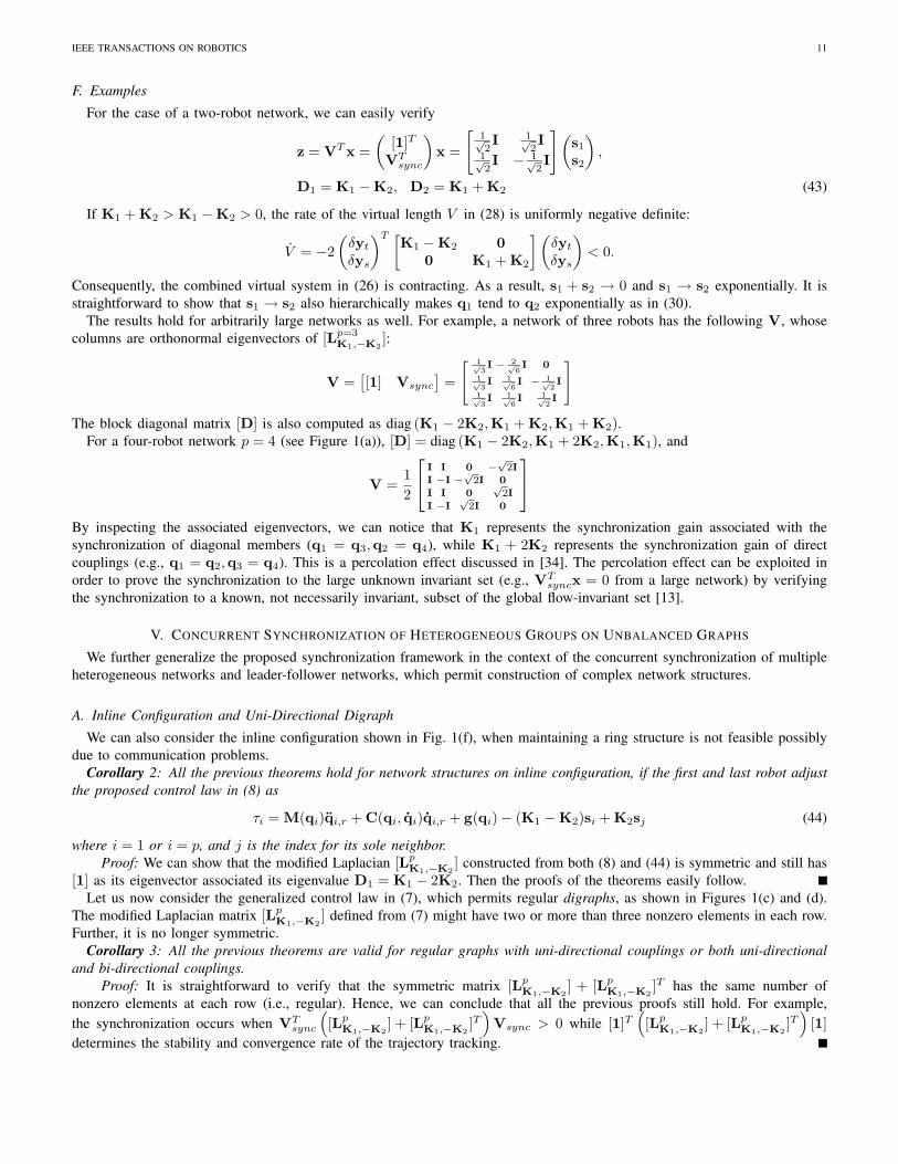
F. Examples

For the case of a two-robot network, we can easily verify

z = VT x =(

[1]T

VTsync

)x =

[1√2I 1√

2I

1√2I − 1√

2I

](s1

s2

),

D1 = K1 −K2, D2 = K1 + K2 (43)

If K1 + K2 > K1 −K2 > 0, the rate of the virtual length V in (28) is uniformly negative definite:

V = −2(δyt

δys

)T [K1 −K2 00 K1 + K2

](δyt

δys

)< 0.

Consequently, the combined virtual system in (26) is contracting. As a result, s1 + s2 → 0 and s1 → s2 exponentially. It isstraightforward to show that s1 → s2 also hierarchically makes q1 tend to q2 exponentially as in (30).

The results hold for arbitrarily large networks as well. For example, a network of three robots has the following V, whosecolumns are orthonormal eigenvectors of [Lp=3

K1,−K2]:

V =[[1] Vsync

]=

[ 1√3I − 2√

6I 0

1√3I 1√

6I − 1√

2I

1√3I 1√

6I 1√

2I

]The block diagonal matrix [D] is also computed as diag (K1 − 2K2,K1 + K2,K1 + K2).

For a four-robot network p = 4 (see Figure 1(a)), [D] = diag (K1 − 2K2,K1 + 2K2,K1,K1), and

V =12

I I 0 −√

2I

I −I −√

2I 0

I I 0√

2I

I −I√

2I 0

By inspecting the associated eigenvectors, we can notice that K1 represents the synchronization gain associated with thesynchronization of diagonal members (q1 = q3,q2 = q4), while K1 + 2K2 represents the synchronization gain of directcouplings (e.g., q1 = q2,q3 = q4). This is a percolation effect discussed in [34]. The percolation effect can be exploited inorder to prove the synchronization to the large unknown invariant set (e.g., VT

syncx = 0 from a large network) by verifyingthe synchronization to a known, not necessarily invariant, subset of the global flow-invariant set [13].

V. CONCURRENT SYNCHRONIZATION OF HETEROGENEOUS GROUPS ON UNBALANCED GRAPHS

We further generalize the proposed synchronization framework in the context of the concurrent synchronization of multipleheterogeneous networks and leader-follower networks, which permit construction of complex network structures.

A. Inline Configuration and Uni-Directional Digraph

We can also consider the inline configuration shown in Fig. 1(f), when maintaining a ring structure is not feasible possiblydue to communication problems.

Corollary 2: All the previous theorems hold for network structures on inline configuration, if the first and last robot adjustthe proposed control law in (8) as

τi = M(qi)qi,r + C(qi, qi)qi,r + g(qi)− (K1 −K2)si + K2sj (44)

where i = 1 or i = p, and j is the index for its sole neighbor.Proof: We can show that the modified Laplacian [Lp

K1,−K2] constructed from both (8) and (44) is symmetric and still has

[1] as its eigenvector associated its eigenvalue D1 = K1 − 2K2. Then the proofs of the theorems easily follow.Let us now consider the generalized control law in (7), which permits regular digraphs, as shown in Figures 1(c) and (d).

The modified Laplacian matrix [LpK1,−K2

] defined from (7) might have two or more than three nonzero elements in each row.Further, it is no longer symmetric.

Corollary 3: All the previous theorems are valid for regular graphs with uni-directional couplings or both uni-directionaland bi-directional couplings.

Proof: It is straightforward to verify that the symmetric matrix [LpK1,−K2

] + [LpK1,−K2

]T has the same number ofnonzero elements at each row (i.e., regular). Hence, we can conclude that all the previous proofs still hold. For example,the synchronization occurs when VT

sync

([Lp

K1,−K2] + [Lp

K1,−K2]T)

Vsync > 0 while [1]T([Lp

K1,−K2] + [Lp

K1,−K2]T)

[1]determines the stability and convergence rate of the trajectory tracking.


Leader

2nd Network

1st

Network

Fig. 3. Concurrent synchronization between two different groups. The desired trajectory inputs are denoted by the dashed-lines whereas the solid linesindicate mutual diffusive couplings. The independent leader sends the same desired trajectory input to the first network group. If we view the dashed-lines asedges of the graph, the network is on an unbalanced graph.

B. Synchronization of Heterogeneous Robots

Consider the proposed control law for a network comprised of heterogeneous dynamics as follows:

τi = Mi(qi)qi,r + Ci(qi, qi)qi,r + gi(qi) (45)−K1(qi − qi,r) + K2(qi−1 − qi−1,r) + K2(qi+1 − qi+1,r)

where Mi, Ci, and gi(qi) represent the i-th robot dynamics, which can be different from robot to robot. Each robot has thesame number of configuration variables (qi ∈ Rn).

Corollary 4: The proposed tracking and synchronization control law in (8) can easily be applied to a network consistingof heterogeneous robots in (2) if the stable tracking condition in Theorem 6 is true.

Proof: The M and C matrix notations used in the previous sections can be interpreted as M(q1) → M1(q1) andM(q2)→M2(q2) with M1(·) 6= M2(·) (the same for the C matrices). Hence, the assumption of non-identical dynamics doesnot alter the proof of exponential tracking in Theorem 5 and stable synchronization in Theorem 6. However, the synchronizationwith indifferent tracking (Theorem 7) is no longer true for non-identical robots since VT

syncx = 0 is not a flow-invariantmanifold, and q1 = q2 does not cancel the off-diagonal terms 1/2 [M1(q1)−M2(q2)] in the metric matrix VT [M]V.

C. Concurrent Synchronization of Heterogeneous Groups

We present a new method of achieving the concurrent synchronization of multiple heterogeneous networks in this section.Such a method can be used to apply the main results in the previous sections to more complex networks, as shown inFigure 1(e). The networks in the figure are neither regular nor balanced due to the reference input couplings. In [34],concurrent synchronization is defined as a regime where the ensemble of dynamical elements is divided into multiple groupsof fully synchronized elements, but elements from different groups are not necessarily synchronized and can exhibit entirelydifferent dynamics.

As discussed in the previous sections, we pay particular attention to the fact that there exist two different time scales ofthe proposed synchronization tracking control law. In particular, one rate is associated with the trajectory tracking (D1), whilethe other represents the convergence rate of the synchronization (D2). This implies that there are two different inputs to thesystem, namely, the common reference trajectory qd(t) and the diffusive couplings with the adjacent members. Accordingly,we exploit a desired trajectory qd(t) to create multiple combinations of different dynamics groups.

For instance, Figure 3 represents the concurrent synchronization of two different dynamic networks. The first network,consisting of four heterogeneous robots, has the diffusive coupling structure proposed by the tracking control law in (8). Theindependent leader sends a desired trajectory command qd(t) to each member of the first network. Note that the dimension ofthe leader dynamics need not be equal to that of the first network, since a signal from the leader can be pre-conditioned. Withan appropriate selection of gains, each dynamics in the first network synchronize while exponentially following the leader.Therefore, the proposed scheme can be interpreted in the context of the leader-follower problem ([17], [23], [49]).

The second network consists of three heterogeneous dynamics, also different from those of the first group. Each elementreceives a different desired trajectory input from the adjacent element of the first network. Again, the desired trajectory inputfor the second group can be pre-conditioned from the first network, resulting in

q2d(t) = f(q1, t) (46)

where q1 is the state vector of the member in the first network that sends in the desired command and f is a differentiablenonlinear function of q1. As a result, the dynamics of the two networks can be entirely different (i.e., q1 ∈ Rm, q2 ∈ Rn,and m 6= n). Note that q2d, needed for the proposed control law in (7), can be obtained from a nonlinear observer [40]. Theconcurrent synchronization between the first and second networks can be proven as follows.


Corollary 5: Consider the network structures that are unbalanced (i.e., the in-degrees are not equal to the out-degrees) dueto the directional reference input connections among the regular balanced graphs, shown as the dashed lines in Figures 1(e)and 3. The robots on such graphs globally exponentially synchronize if the individual groups synchronize from Theorems 5and 6.

Proof: For the example shown in Figure 3, once the first network synchronizes, the second network also ends up receivingthe same desired trajectory to follow, while they interact to synchronize exponentially fast. Accordingly, we can achieveconcurrent synchronization between two different network groups. The proof of Theorem 6 holds until (30), where now thedesired trajectory inputs are different for each robot. Then, we can conclude that the robots in the second network synchronize,if the desired reference inputs q2d,i, 1 ≤ i ≤ p, sent from the first network, synchronize:

VTsync{q2}+

(VT

sync[Λ]Vsync

)VT

sync{q2} (47)

−(VT

sync[rT1 , · · · , rT

p ]T → 0)

= VTsyncx2 → 0

where ri = q2d,i + Λq2d,i, and x2 is the vector of the composite variables (si) of the second network. If the first networksynchronizes, the reference trajectory term vanishes (VT

sync[rT1 , · · · , rT

p ]T → 0), thereby ensuring the synchronization ofthe second network (i.e., VT

sync{q2} → 0). This can be extended to arbitrarily large groups of synchronized dynamics byappropriately assigning the desired trajectory inputs and the diffusive couplings.

Remark 7: The previous example in Figure 3 and Corollary 5 can be interpreted in terms of feedback hierarchies (seeTheorem 2). The first network in the figure provides feedforward commands to the second network, but does not receiveany command from the second network. Note that the dynamics at each level can be very different, in order to construct adynamic concurrent combination of heterogeneous networks. Since the feedforward inputs can be appropriately scaled andconditioned, the dimensions between hierarchical layers can also be very different. For example, the dynamics higher in thehierarchy need not be oscillators, but could be systems with multiple equilibria (e.g., x = −∇V , with local minima in V [41]),with synchronization corresponding to convergence toward a common minimum. Concurrent synchronization discussed in thissection can be exploited to construct a large complex network consisting of heterogeneous dynamics such as robots, groundvehicles, and unmanned aerial vehicles.

VI. EXTENSIONS

Let us further extend the proposed control law.

A. Synchronization of Robots Using Linear PD Control

One may consider the following Proportional and Derivative (PD) coupling control law for two identical robots from (2)with p = 2,

τ1 = −K1(q1 + Λq1) + K2(q2 + Λq2)τ2 = −K1(q2 + Λq2) + K2(q1 + Λq1)

(48)

where qi = qi − qd and the bounded reference position qd has zero velocity such that ˙qi = qi.For simplicity, the gravity term in (2) is assumed to be zero or canceled by a feed-forward control law. Then, the closed-loopdynamics satisfy

M(q1)q1 + C(q1, q1)q1 + Kq1 + KΛq1 = u(t)M(q2)q2 + C(q2, q2)q2 + Kq2 + KΛq2 = u(t)

(49)

where K = K1 + K2 and u(t) = K2(q1 + q2) + K2Λ(q1 + q2).Similar to Section IV-C, we can perform a spectral decomposition:(

VT [M]V)VT x +

(VT [C]V

)VT x (50)

+(VT [Lp

K1,−K2]V)

VT x +(VT [Lp

K1Λ,−K2Λ]V)

VT x = 0

Using the following Lyapunov function, it is straightforward to show that this PD coupling control law drives the system tothe desired rest state qd globally and asymptotically while tending to the synchronized flow-invariant manifold:

V =12

(qp

qm

)T [M1+M22

M1−M22

M1−M22

M1+M22

](qp

qm

)(51)

+12

(qp

qm

)T [(K1 −K2)Λ 00 (K1 + K2)Λ

](qp

qm

)where M1 = M(q1), M2 = M(q2), VT x =

(qp

qm

)= 1√

2

(q1 + q2

q1 − q2

), qp = 1√

2(q1 + q2).


The rate of V can be computed as

dV

dt= −

(qp

qm

)T [K1 −K2 00 K1 + K2

](qp

qm

)≤ 0 (52)

which implies that V is negative semi-definite with K1 + K2 > 0 and K1 −K2 > 0.By invoking LaSalle’s invariant set theorem [40], we can conclude that qp, qp, qm, and qm tend to zero with global and

asymptotic convergence. This implies that q1 and q2 will follow qd while q1 and q2 synchronize asymptotically from anyinitial condition. This can be extended to arbitrarily large networks as shown in Figure 1.

Note that if Λ = 0, the PD coupling control law in (48) reduces to velocity coupling

τ1 = −K1q1 + K2q2, τ2 = −K1q2 + K2q1 (53)

This velocity coupling control can also be derived from the exponential tracking control law in (8) by setting qd = 0, qd = 0,and Λ = 0. Therefore, the proof of the linear PD synchronization with Λ = 0 is the same as Section IV-C whereas theconvergence rate is now exponential compared with the asymptotic convergence of the PD control. On the other hand, we canfind that positions do not synchronize in the absence of the gravity term even though the velocities synchronize exponentiallyfast.

B. Synchronization with Limited Communication Bandwidth

We now consider multiple dynamics with partially coupled joints (or partially coupled variables). For example, we can assumethat only the lower joint is coupled in a two-robot system having two joint variables with q = (x1, x2)T for (i = 1, j = 2) or(i = 2, j = 1):

τi = M(qi)qi,r + C(qi, qi)qi,r + g(qi)−K1si

+ K2

( ˙x1

0

)qj

+ K2Λ(x1

0

)qj

(54)

Nevertheless, Theorems 5 and 6 are true with diagonal matrices, K1, K2 and Λ, which can be verified by writing theclosed-loop system as in (17):

M(q1)s1 + C(q1, q1)s1 + (K1 + K2P)s1 = u(t) (55)M(q2)s2 + C(q2, q2)s2 + (K1 + K2P)s2 = u(t)

u(t) = K2P(s1 + s2), P = diag(1, 0)

It is straightforward to prove that Theorems 5 and 6 still hold. This is because (K1+K2P) and (K1−K2P) are still uniformlypositive definite, enabling exponential synchronization and exponential convergence to the desired trajectory, respectively.Hence, we did not break any assumption in the proof of Theorem 6. This partial-state coupling also works for the semi-contracting case with (34), as presented in Section IV-D. While the coupled variables synchronize to the weighted average ofthe initial conditions, the uncoupled variables synchronize to zero.

C. Synchronization with Time-Delays

The results may be extended to time-delayed couplings (see also [4]). Consider for instance the two-robot dynamics (17),which becomes

M(q1)s1 + C(q1, q1)s1 + (K1 −K2)s1 = τ21

M(q2)s2 + C(q2, q2)s2 + (K1 −K2)s2 = τ12

τ21 = K2(s2(t− T )− s1(t)) (56)τ12 = K2(s1(t− T )− s2(t))

where the constant T > 0 denotes the communication delay between the two robots. The robots are programmed to followthe same predefined trajectory qd(t) such that si(t− T ) = qi(t− T ) + Λqi(t− T )− (qd(t) + Λqd(t)) for any i.

Theorem 9: The robots in (56) synchronize globally asymptotically ∀T > 0 under the assumptions of Theorem 6.Proof: Similar to [42], [48], consider the differential length

V = δzT(VT [M]V

)δz +

∫ t

t−T

δzT (ε)[

K2 00 K2

]δz(ε)dε (57)


0 1 2 3 4 5 6 7 8.5

1

.5

0

.5

1

.5

2

s[m]

Robot 1

Robot 2

Robot 3

Robot 4

(a) Simulation result.

0 5 10 15 20 25 30 35 40

−0.4

−0.2

0

0.2

0.4

s [m

]

Tracking errors of four−robot network

0 5 10 15 20 25 30 35−1.5

−1

−0.5

0

Join

t 1 [r

ad]

Robot1Robot2Robot3Robot4

0 5 10 15 20 25 30 35 40

0

0.5

1

1.5

2

time [s]

Join

t 2 [r

ad]

(b) Tracking error of each robot

Fig. 4. Synchronization of a four-robot network

Using (56) shows that V is negative semi-definite,

V =− 2δzT[

K1−K2 00 K1−K2

]δz (58)

− δτT21K

−12 δτ21 − δτT

12K−12 δτ12

Note that K1 + K2 > K1 −K2 > 0 implies K2 > 0.Also, V is bounded. By Barbalat’s lemma, V tends to zero globally asymptotically, which in turn implies δz→ 0, δτ21 →

0, δτ12 → 0. Hence, the solutions converge to a single trajectory asymptotically. Since s1(t− T ) = s2(t− T ) is a particularsolution of (56) and the desired trajectory qd(t) is the same for each robot, q1(t) and q2(t) globally asymptotically synchronizeregardless of T .

D. A Perspective on Model Reduction by Synchronization

Another benefit of exponential synchronization is its implication for model reduction [8]. Exponential synchronization ofmultiple nonlinear dynamics allows us to reduce the dimensionality of the stability analysis of a large network. As notedearlier, the synchronization rate (D2) is faster than the tracking rate (D1). Assuming that the dynamics are synchronized, theaugmented dynamics in (14) reduces to

M(q)s + C(q, q)s + (K1 − 2K2)s = 0 (59)

where q = q1 = · · · = qp, and D1 = K1 − 2K2 is replaced by K1 −K2 for p = 2.This implies that once components of a network are shown to synchronize, we can regard them as a single dynamics of reduceddimension, which simplifies any additional stability or perturbation analysis.

VII. SIMULATION RESULTS

A. Tracking Synchronization of Four Robots

Even though the local coupling structure of (7) and (8) has been emphasized, the difference from all-to-all coupling is notevident in a network comprised of less than four members (p ≤ 3). To illustrate the effectiveness of the proposed scheme for arobot network with p ≥ 4, a network of four identical 3-DOF robots is considered here (see Fig 1(a)). The dynamics modelingof the 3-DOF robot is based upon the double inverted pendulum robot on a cart (see Fig. 4(a)), and each joint is assumed tobe frictionless. The physical parameters of each robot are given in [7].

The simulation result is presented in Figure 4. The four identical robots, initially at some arbitrary initial conditions, aredriven to synchronize as well as to track the time-varying desired trajectory: sd(t) = 0.2t, θ1d(t) = cos(0.02πt), θ2d(t) =π/4(1 − cos(0.08πt)). For the control gains in the control law (8), we used K1 = 5I, K2 = 2I, and Λ = 5I. Accordingto Theorems 5 and 6, the tracking gain K1 − 2K2 is smaller than the corresponding synchronization gains K1 + 2K2 andK1. Figure 4(b) shows the tracking errors of the four robots. We can see that the robots synchronize exponentially fast fromarbitrary initial conditions, and this synchronization occurs faster than the exponential convergence of tracking errors. Sucha result can be useful to rapidly achieve a collective motion of multiple robots in the presence of external disturbances. IfK1 = 2K2 instead, we can easily show that the robots synchronize with global exponential convergence, although the trackingerrors will not tend to zero.


5

3

21

6 4

9

10

8

7

2

1

3

(a) Three networks connected by feedback hierarchies.

0 5 10 15 20 25 30 35 40−0.6−0.4−0.2

00.20.4

s [m

]

Tracking errors of ten−robot network

0 5 10 15 20 25 30 35 40−1.5

−1

−0.50

Join

t 1 [r

ad]

0 5 10 15 20 25 30 35 40

0

1

2

time [s]

Join

t 2 [r

ad]

(b) Tracking error of each robot

Fig. 5. Synchronization of ten robots on three heterogeneous networks

B. Simulation of Concurrent Synchronization for Ten Robots

Let us consider three heterogeneous networks connected by feedback hierarchies shown in Fig. 5(a). If we view the referencetrajectory inputs (dashed lines in the figure) as edges of the graph, as discussed in Section V, this graph is unbalanced. The firstnetwork (robot 1 through 4) is identical to the network of four 3-DOF robots in the previous section. All the physical parametersof the second network (robot 5 through 7) are twice larger than those of the first network while those of the third network are1.5 times larger. Also, note that the third network is on an inline configuration by connecting the second feedback gain K2 ofthe control law in (8) back to itself. All the previous theorems still hold for such an inline configuration (see Corollary 2). Asseen in Fig. 5(b), the first, second, and third network individually synchronize robots within each network from arbitrary initialconditions. The first and second network also follow the reference trajectory command from the adjacent members. For thereference trajectory commands, we assume that we can send the position and velocity values (qd, qd). Then, qd is estimated bya high pass filter. Eventually, all the robots exponentially synchronize and then follow the desired trajectory staying together.This concurrent synchronization can be used to construct a complex and large-scale dynamic network consisting of an arbitrarynumber of heterogeneous robots and networks.

C. Simulation of Adaptive Synchronization

We assess the effectiveness of the proposed adaptive synchronization control law presented in Section IV-E. Consider atwo-robot network, comprised of the two-link manipulator robots given in page 396 of [40]. The desired trajectory for thefirst joint is θ1d(t) = sinπt and for the second joint is θ2d(t) = 2(1 − cos 0.6πt). The initial parameter estimates for bothrobots are defined as a(0) = (3, 1, 1, 1)T , and Γ = diag(0.03, 0.05, 0.1, 0.3). Figure 6(a) shows the synchronization of thetwo robots with stable tracking by K1 = 20I, K2 = 15I, and Λ = 10I. Hence, the synchronization gain K1 + K2 is largerthan the tracking gain K1 −K2. Note that the synchronization of the tracking errors implies the synchronization of the statevariables (i.e., joint 1 and joint 2). As discussed before, the synchronization occurs faster than the tracking. This simulationresult indicates that the proposed adaptive control law can be used to synchronize motions of robots with unknown physicalparameters.

In contrast, Figure 6(b) shows the synchronization with indifferent tracking by the gains of K1 = K2 = 20I and Λ = 10I.The tracking dynamics then have zero gain (indifferent). So the two robots synchronize asymptotically, while the tracking errorsremain within a finite ball. In both cases (Figs. 6(a) and (b)), the proposed adaptive control law ensures neither the asymptoticconvergence nor the synchronization of the physical parameter estimates ai, unless the persistency of excitation condition is met.Nevertheless, the robots synchronize asymptotically from any initial condition in the presence of such parametric uncertainty.This adaptive version makes the proposed synchronization framework more practical. It should also be obvious to readers thatthe proposed control law can be straightforwardly extended to robust adaptive control schemes based on sliding control [40].

VIII. CONCLUSIONS

We have presented the new synchronization tracking control law that can be directly applied to cooperative control ofmulti-robot systems and oscillation synchronization in robotic manipulation and locomotion. We have also shown that complexdynamic networks can be constructed by exploiting concurrent synchronization such that multiple groups of fully synchronizedelements coexist. The proposed decentralized control law, which requires only local coupling feedback for global exponentialconvergence, eliminates both the all-to-all coupling and the feedback of the acceleration terms, thereby reducing communicationburdens and complexity. Furthermore, in contrast with prior work which used simple single or double integrator models, theproposed method permits highly nonlinear systems. Providing exact nonlinear stability results constitutes one of the maincontributions of this paper; global and exponential stability of the closed-loop system has been derived by using contraction


0 5 10 15 20 25

−1

−0.5

0

0.5

time[s]

Tra

ckin

g E

rror

[rad

]Synchronization with Asymptotic Tracking

0 5 10 15 20 25−6

−4

−2

0

2

4

time[s]

Par

amet

er E

stim

ates

#1:θ1 #1:θ2 #2:θ1 #2:θ2

#1: a1 a2 a3 a4 #2:a1 a2 a3 a4

(a) with asymptotically stable tracking

0 5 10 15 20 25

−1

−0.5

0

0.5

time[s]

Tra

ckin

g E

rror

[rad

]

Synchronization with Indifferent Tracking

0 5 10 15 20 25−6

−4

−2

0

2

4

6

time[s]

Par

amet

er E

stim

ates

#1:θ1 #1:θ2 #2:θ1 #2:θ2

#1: a1 a2 a3 a4 #2:a1 a2 a3 a4

(b) with indifferent tracking

Fig. 6. Adaptive synchronization of two two-link manipulator robots

theory. Contraction analysis, overcoming a local result of Lyapunov’s indirect method, yields global results based on differentialstability analysis. While we have focused on the mutual synchronization problem where synchronization and trajectory trackingtake place simultaneously, the proposed method has also been shown to be a generalization of the average consensus problemthat does not address trajectory tracking. It has been emphasized that there exist multiple time scales in the closed-loopsystems: the faster convergence rates represents the transient boundary layer dynamics of synchronization while the slowerrate determines how fast the synchronized systems track the common reference trajectory. Exponential synchronization with afaster convergence rate enables reduction of multiple dynamics into a simpler form, thereby simplifying the stability analysis.

Simulation results show the effectiveness of the proposed control strategy. The proposed bi-directional coupling has alsobeen generalized to permit partial-state coupling and uni-directional coupling. Further extensions to proportional-derivativecoupling, adaptive synchronization, time-varying network topology, and concurrent synchronization of multiple heterogeneousnetworks on unbalanced graphs exemplify the benefit of the proposed approach based on contraction theory.

ACKNOWLEDGEMENTS

This paper benefited from constructive comments from the associate editor, anonymous reviewers, Dr. Keehong Seo, andProf. David W. Miller at MIT.

REFERENCES

[1] S. Arimoto, F. Miyasaki, H. G. Lee, and S. Kawamura, “Revival of Lyapunovs direct method in robot control and design,” in Proc. American ControlConf., Atlanta, GA, June 1988, pp. 1764–1769.

[2] S. Arimoto, Control Theory of Nonlinear Mechanical Systems: A Passivity-based and circuit-theoretic approach, Oxford University Press, Oxford, UK,1996.

[3] N. Chopra and M. W. Spong, “On synchronization of networked passive systems with time delays and application to bilateral teleoperation,” Proceedingsof the SCIE Annual Conference, Okayama, Japan, August 8-10, 2005, pp. 3424-3429.

[4] N. Chopra and M. W. Spong, “Passivity-based control of multi-agent systems,” in Advances in Robot Control: From everyday physics to human-likemovements, Sadao Kawamura and Mikhail Svinin, Editors, Springer-Verlag, Berlin, 2006, pp. 107–134.

[5] F. Chung, Spectral Graph Theory, Number 92 in CBMS Regional Conference Series in Mathematics, American Mathematical Society, 1997.[6] S.-J. Chung and J.-J. E. Slotine, “Cooperative robot control and synchronization of Lagrangian systems,” Proc. 46th IEEE Conf. on Decision and Control,

New Orleans, LA, Dec. 2007, pp. 2504–2509.[7] S.-J. Chung, “Nonlinear control and synchronization of multiple Lagrangian systems with application to tethered formation flight spacecraft,” Doctor of

Science Thesis, Dept. of Aeronautics and Astronautics, Massachusetts Inst. of Technology, Cambridge MA, 2007.[8] S.-J. Chung, J.-J. E. Slotine, and D. W. Miller, “Nonlinear model reduction and decentralized control of tethered formation flight,” Journal of Guidance,

Control, and Dynamics, Vol. 30, No. 2, pp. 390–400, Mar.–Apr. 2007.[9] S.-J. Chung, U. Ahsun, and J.-J. E. Slotine, “Application of synchronization to formation flying spacecraft: Lagrangian approach,” to be published.,

Journal of Guidance, Control and Dynamics, Vol. 32, No. 2, Mar.–Apr. 2009.[10] B. P. Demidovich, “Dissipativity of a nonlinear system of differential equations,” ser. matematika mehanika, part I N.6, pp. 19–27, Vestnik Moscow

State University, 1962.[11] B. P. Demidovich, “Dissipativity of a nonlinear system of differential equations,” ser. matematika mehanika, part II N.1, pp.3–8, Vestnik Moscow State

University, 1962.[12] R. Fierro, P. Song, A. Das, and V. Kumar, “Cooperative control of robot formations,” in Cooperative Control and Optimization: Series on Applied

Optimization, Kluwer Academic Press, pp. 79–93, 2002.[13] L. Gerard and J.-J. E. Slotine, “Neuronal networks and controlled symmetries, a generic framework,” arXiv:q-bio/0612049v4 [q-bio.NC], 29 March

2008. Available: http://arxiv.org/abs/q-bio/0612049[14] P. Hartmann, Ordinary Differential Equations, John Wiley & Sons, New York, 1964.


[15] A. J. Ijspeert, A. Crespi, and J.-M. Cabelguen, “Simulation and robotics studies of salamander locmotion: applying neurobiological principles to thecontrol of locomotion in robotics,” Neuroinformatics, Vol. 3, No. 3, pp. 171–196, Sept. 2005.

[16] I.-A. F. Ihle, M. Arcak, and T. I. fossen, “Passivity-based designs for synchronized path-following,” Automatica, Vol. 43, No. 9, pp. 1508–1518, Sept.2007.

[17] A. Jadbabaie, J. Lin, and A. S. Morse, “Coordination of groups of mobile autonomous agents using nearest neighbor rules,” IEEE Trans. on AutomaticControl, Vol. 48, No. 6, pp. 988–1001, June 2003.

[18] J. Jouffroy and J.-J. E. Slotine, “Methodological remarks on contraction theory,” IEEE Conf. on Decision and Control, Atlantis, Paradise Island, Bahamas,Vol. 3, Dec. 2004, pp. 2537–2543.

[19] H. K. Khalil, Nonlinear Systems, 3rd Ed., Prentice Hall, Upper Saddle River, NJ, 2002, pp. 339–350.[20] K. Krstic, I. Kanellakopoulos, and P. Kokotovic, Nonlinear and Adaptive control Design, John Wiley and Sons, New York, NY, 1995, pp. 21–29.[21] D. Lee and P. Y. Li, “Formation and maneuver control of multiple spacecraft,” Proc. of the 2003 American Control Conf., Vol. 1, June 2003, pp. 278–283.[22] D. Lee and M. W. Spong, “Stable flocking of multiple inertial agents on balanced graph,” Proc. of the 2006 American Control Conf., Vol. 52, June

2006, pp. 1469–1475.[23] N. E. Leonard and E. Fiorelli, “Virtual leaders, artificial potentials and coordinated control of groups,” Proc. 40th IEEE Conf. on Decision and Control,

2001, pp. 2968–2973.[24] D. C. Lewis, “Metric properties of differential equations,” American Journal of Mathematics, Vol. 71, pp. 294–312, 1949.[25] Z. Lin, M. Broucke, and B. Francis, “Local control strategies for groups of mobile autonomous agents,” IEEE Trans. on Automatic Control, Vol. 49,

No. 4, pp. 622–629, Apr. 2004.[26] W. Lohmiller and J.-J. E. Slotine, “On contraction analysis for nonlinear systems,” Automatica, Vol. 34, No. 6, pp. 683-696, June 1998.[27] W. Lohmiller and J.-J. E. Slotine, “High-order nonlinear contraction analysis,” MIT Nonlinear Systems Laboratory (NSL) Report, NSL-050901.[28] M. Mesbahi and F. Y. Hadaegh, ”Formation flying of multiple spacecraft via graphs, matrix inequalities, and switching,” Journal of Guidance, Control,

and Dynamics, Vol. 24, No. 2, pp. 369–377, Mar.–Apr. 2001.[29] G. Niemeyer and J.-J. E. Slotine, “Telemanipulation with time delays,” Int. J. of Robotics Research, Vol. 23, No. 9, pp. 873–890, Sept. 2004.[30] R. Olfati-Saber and R. M. Murray, “Consensus problems in networks of agents with switching topology and time-delays,” IEEE Trans. on Automatic

Control, Vol. 49, No. 9, pp. 1520–1533, Sep. 2004.[31] P. Ogren, M. Egerstedt, and X. Hu, “A control Lyapunov function approach to multiagent coordination,” IEEE Trans. on Robotics and Automation, Vol.

18, No. 5, pp. 847–851, Oct. 2002.[32] P. Ogren, E. Fiorelli, and N. E. Leonard, “Cooperative control of mobile sensor networks: adaptive gradient climbing in a distributed environment,”

IEEE Trans. on Automatic Control, Vol. 49, No. 8, pp. 1292–1302, Aug. 2004.[33] D. A. Paley, N. E. Leonard, R. Sepulchre, D. Grunbaum, and J. K. Parrish, “Oscillator models and collective motion: spatial patterns in the dynamics

of engineered and biological networks,” IEEE Control Systems Magazine, Vol. 27, No. 4, pp. 89–105, Aug. 2007.[34] Q.-C. Pham and J.-J. E. Slotine, “Stable concurrent synchronization in dynamic system networks,” Neural Networks, Vol. 20, No. 1, pp. 62–77, Jan.

2007.[35] A. Pitti, M. Lungarella, and Y. Kuniyoshi, “Synchronization: adaptive mechanism linking internal and external dynamics,” Proc. of the 6th Int. Workshop

on Epigenetic Robotics, Paris, France, Sept. 2006.[36] W. Ren, “Multi-vehicle consensus with a time-varying reference state,” Systems & Control Letters, Vol. 56, No. 7-8, pp. 474–483, July 2007.[37] W. Ren, R. W. Beard, and E. Atkins, “Information consensus in multivehicle cooperative control: collective group behavior through local interaction,”

IEEE Control Systems Magazine, Vol. 27, No. 2, pp. 71–82, Apr. 2007.[38] A. Rodriguez-Angeles and H. Nijmeijer, “Mutual synchronization of robots via estimated sate feedback: a cooperative approach,” IEEE Trans. on Control

Systems Technology, Vol. 12, No. 4, pp. 542–554, July 2004.[39] K. Seo, S.-J. Chung, and J.-J. E. Slotine, “CPG-based control of a turtle-like underwater vehicle,” Proc. of the Robotics: Science and Systems (RSS),

Switzerland, June 2008.[40] J.-J. E. Slotine and W. Li, Applied Nonlinear Control, Prentice Hall,. New Jersey, 1991.[41] J.-J. E. Slotine, “Modular stability tools for distributed computation and control,” Int. J. Adaptive Control and Signal Processing, Vol. 17, No. 6, pp.

397–416, 2003.[42] J.-J. E. Slotine and W. Lohmiller, “Modularity, evolution, and the binding problem: a view from stability theory,” Neural Networks, Vol. 14, No. 2, pp.

137–145, Mar. 2001.[43] J.-J. E. Slotine, W. Wang, and K. El Rifai, “Synchronization in networks of nonlinearly coupled continuous and hybrid oscillators,” Proc. of the 6th

International Symposium on Mathematical Theory of Networks and Systems (MTNS 2004), Katholieke Universiteit Leuven, Leuven, Netherlands, Jul.5–9, 2004.

[44] G. Strang, Introduction to Applied Mathematics, Wellesley-Cambridge Press, Wellesey, MA, 1986.[45] D. Sun and J. K. Mills, “Adaptive synchronized control for coordination of multi-robot assembly tasks,” IEEE Trans. on Robotics and Automation, Vol.

18, No. 4, pp. 498–510, Aug. 2002.[46] D. Sun, L. Ren, J. K. Mills, and C. Wang, “A synchronous tracking control of parallel manipulators using cross-coupling approach,” Int. J. of Robotics

Research, Vol. 25, No. 11, pp. 1137–1147, Nov. 2006.[47] W. Wang and J.-J. E. Slotine, “On partial contraction analysis for coupled nonlinear oscillators,” Biological Cybernetics, Vol. 92, No. 1, pp. 38-53, Jan.

2005.[48] W. Wang and J.-J. E. Slotine, “Contraction analysis of time-delayed communications and group cooperation,” IEEE Trans. on Automatic Control, Vol.

51, No. 4, pp. 712–717, Apr. 2006.[49] W. Wang and J.-J. E. Slotine, “A theoretical study of different leader roles in networks,” IEEE Trans. on Automatic Control, Vol. 51, No. 7, pp. 1156–1161,

Jul. 2006.

Soon-Jo Chung (M’06) received the B.S. degree “summa cum laude” from Korea Advanced Institute of Science and Technology,Daejeon, Korea, in 1998, and the S.M. degree in aeronautics and astronautics and the Sc.D. degree in estimation and control fromMassachusetts Institute of Technology (MIT), Cambridge, in 2002 and 2007, respectively. He is currently an Assistant Professor ofaerospace engineering and electrical and computer engineering at Iowa State University, Ames. His current research interests includebio-inspired aerospace robotics, nonlinear control theory, unmanned aerial vehicles, formation flying spacecraft, multivehicle control,and vision-based navigation. Prof. Chung received an Air Force Office of Scientific Research Young Investigator Award in 2008 forhis research on flapping flying microaerial vehicles.


Jean-Jacques E. Slotine was born in Paris, in 1959. He received the Ph.D. degree from Massachusetts Institute of Technology (MIT),Cambridge, in 1983. After working in the Computer Research Department at Bell Labs, in 1984, he joined the faculty at MIT, wherehe is now Professor of Mechanical Engineering and Information Sciences, Professor of Brain and Cognitive Sciences, and Directorof the Nonlinear Systems Laboratory. He is the coauthor of the textbooks Robot Analysis and Control (Wiley, 1986) and AppliedNonlinear Control (Prentice-Hall, 1991). Prof. Slotine was a Member of the French National Science Council from 1997 to 2002.

ieee transactions on robotics 1 cooperative …web.mit.edu/nsl/www/preprints/robot_sync_09.pdf ·...

Documents