ieee transactions on visualization and computer … · mediate visualization, the wavelet clusters...

Multiscale Time Activity Data Exploration viaTemporal Clustering Visualization Spreadsheet

Jonathan Woodring and Han-Wei Shen

Abstract—Time-varying data is usually explored by animation or arrays of static images. Neither is particularly effective for classifying

data by different temporal activities. Important temporal trends can be missed due to the lack of ability to find them with current

visualization methods. In this paper, we propose a method to explore data at different temporal resolutions to discover and highlight

data based upon time-varying trends. Using the wavelet transform along the time axis, we transform data points into multiscale time

series curve sets. The time curves are clustered so that data of similar activity are grouped together at different temporal resolutions.

The data are displayed to the user in a global time view spreadsheet, where she is able to select temporal clusters of data points and

filter and brush data across temporal scales. With our method, a user can interact with data based on time activities and create

expressive visualizations.

Index Terms—Time-varying, time histogram, filter banks, wavelet, animation, transfer function, clustering, K-means, visualization

spreadsheet.

Ç

1 INTRODUCTION

DATA points in a time-varying data set exhibit differentactivities over time, which characterize the temporal

trends of underlying features. We define a temporal trendas the characterization of the change in value of a data pointover time in a series. This can be classified in a variety ofways, such as when a trend begins, when it ends, the rate ofchange, and the value over time. This is true for all time-varying data sets, and it seems natural to classify datapoints based upon their activity to find temporal hot spots.

Traditional data exploration deals with classificationbased upon temporally static value quantities. When time isnot considered, patterns and correlations based on temporalactivity can be missed. For example, in animation ofvolumes, if the transfer function does not map a changeover time to a visible range or the mapping does nothighlight the dynamic activity, the user will miss thechange, or it will go ignored. It has been noted that changeblindness can occur when visually perceptual phenomenachange too slowly to be detected [23]. For rendering a singletime step, most methods do not have a concept of mappingbased on time activities or intercorrelated time activities.

Only until recently has scientific visualization attemptedto tackle classification based upon temporal activity. Fanget al. developed a system to classify and segment medical databased on a distance metric from the time activity curve vector[5]. Akiba et al. [1], [2] use the time histogram to create time-varying transfer functions based upon the time profile of adata set. Our method builds upon these concepts to facilitate

time-varying data exploration, such that the data areexplored and classified based upon multiscale temporalactivities.

Our goal is to allow explorative capability to find trends ofdifferent temporal scales in data to create visualizations basedon temporal activity. Similar to multiscale spatial classifica-tion [20], temporal activity can occur at different temporalscales. To explore the data, we utilize the wavelet [19] totransform data points into a set of time series curves groupedinto different wavelet or filter bank levels. By filtering the datainto different frequency bands, a user is able to visualize herdata at different scales of activity and find data that sharesimilar temporal trends at particular time scale.

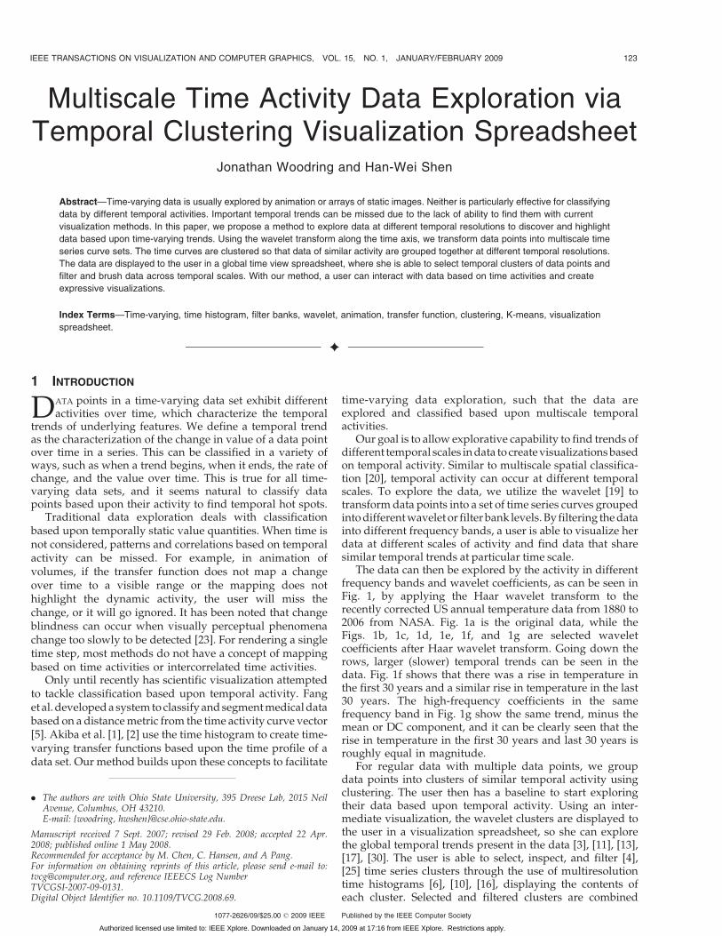
The data can then be explored by the activity in differentfrequency bands and wavelet coefficients, as can be seen inFig. 1, by applying the Haar wavelet transform to therecently corrected US annual temperature data from 1880 to2006 from NASA. Fig. 1a is the original data, while theFigs. 1b, 1c, 1d, 1e, 1f, and 1g are selected waveletcoefficients after Haar wavelet transform. Going down therows, larger (slower) temporal trends can be seen in thedata. Fig. 1f shows that there was a rise in temperature inthe first 30 years and a similar rise in temperature in the last30 years. The high-frequency coefficients in the samefrequency band in Fig. 1g show the same trend, minus themean or DC component, and it can be clearly seen that therise in temperature in the first 30 years and last 30 years isroughly equal in magnitude.

For regular data with multiple data points, we groupdata points into clusters of similar temporal activity usingclustering. The user then has a baseline to start exploringtheir data based upon temporal activity. Using an inter-mediate visualization, the wavelet clusters are displayed tothe user in a visualization spreadsheet, so she can explorethe global temporal trends present in the data [3], [11], [13],[17], [30]. The user is able to select, inspect, and filter [4],[25] time series clusters through the use of multiresolutiontime histograms [6], [10], [16], displaying the contents ofeach cluster. Selected and filtered clusters are combined

IEEE TRANSACTIONS ON VISUALIZATION AND COMPUTER GRAPHICS, VOL. 15, NO. 1, JANUARY/FEBRUARY 2009 123

. The authors are with Ohio State University, 395 Dreese Lab, 2015 NeilAvenue, Columbus, OH 43210.E-mail: {woodring, hwshen}@cse.ohio-state.edu.

Manuscript received 7 Sept. 2007; revised 29 Feb. 2008; accepted 22 Apr.2008; published online 1 May 2008.Recommended for acceptance by M. Chen, C. Hansen, and A Pang.For information on obtaining reprints of this article, please send e-mail to:[email protected], and reference IEEECS Log NumberTVCGSI-2007-09-0131.Digital Object Identifier no. 10.1109/TVCG.2008.69.

1077-2626/09/$25.00 � 2009 IEEE Published by the IEEE Computer Society

Authorized licensed use limited to: IEEE Xplore. Downloaded on January 14, 2009 at 17:16 from IEEE Xplore. Restrictions apply.

together into a visualization by using Boolean operations,time series operators, and animation [29], [30], [31].

2 RELATED WORK

We utilize the wavelet to decompose time series data into aseries of wavelet or filter bank levels. Wavelets have beenused previously as a compression and level-of-detailreduction [19] scheme for large data sets. Recently, Lumand Ma have used filter banks as a method to classifyspatial data based on different frequency ranges [20]. Ininformation visualization, the Fourier transform is used todecompose line graphs into different scales to do optimalbanking to 45 at different temporal resolutions, wherebanking to 45 attempts to find an optimal aspect ratio for2D graphs to maximize the angles between line segments to45 degrees for perceptual visualization enhancement. [8].We use the wavelet transform to extract multiresolutiontemporal trends. There has been a use of multiresolutionhistograms for image recognition and matching [6], [10].Jain and Merchant apply the wavelet transform to the colorhistograms for images to build multiresolution histogrampyramids for image retrieval. Hadjidemetriou et al. applyspatial image filtering to acquire multiresolution histogramsfor image matching. Our use of multiscale time histogramsis most like the latter, we filter the data along the time axisand use clustering [7], [15] to match temporal trends.

Brushing, linking, and multiple data views have beenused in the visualization as a means to be able to draw

conclusions between multivariate data. GGobi and the likeare the latest incarnations of multivariate data brushing andlinking [4], [25]. Our use of brushing and linking is appliedin the selection of data points across temporal scales. Theuse of spreadsheet formats are likewise used throughoutvisualization to simultaneously display multiviews of data[3], [11], [13], [17], [30]. We use visualization spreadsheets topresent the data that are acquired through wavelettransformation and clustering. The use of graphical widgetsand user interfaces for are prevalent in classification andtransfer function design [14]. The combination of wavelettransformation, clustering, time histograms, and brushingand linking create a complete user interface to explore andclassify data by temporal activity.

There have been various research efforts in visualizingtime series data in the area of information visualization. Forinstance, van Wijk and van Selow combined cluster analysisand calendar based visualization to identify standard dailypatterns throughout the year [28]. Weber et al. [27]proposed a method to visualize time-series data based onspirals. The spiral graphs are effective for detecting periodicpatterns for large-scale data sets. Hochheiser and Shneider-man [9] proposed a Timebox widget to specify queryconstrains on time series data. Lin et al. [18] introducedVisTree, a time series pattern discovery and visualizationsystem to help analyze data from aerospace applications.

Creating transfer functions and visualizing time-varyingvolumetric data is one recent interest [21]. There has alsobeen other work in automatic and semiautomatic methodsof transfer function creation for time varying data sets [12],[22], [26]. More recently, Akiba et al. have used timehistograms to be able to classify data based upon their timeseries profile [1], [2], [16]. Their method is better at featuretracking over space. Akiba et al.’s assumption is that datapoint populations will aggregate in value space and movetogether in value space. In this paper, we make theassumption that interesting data points have similartemporal trends. While our method is better at findingand isolating data points based on similar activity, weutilize their method for creating dynamic transfer functionsfor data points based on extracted temporal features. Ourassumption is more closely linked to that by Fang et al. [5].They use a method to segment medical data based uponcalculating distance metrics from a time series profile curve[5]. We also extract data points based on time activity butacross several temporal scales with the ability to query andexplore at different resolutions. This work of temporalactivity selection provides the data input to volumecombination methods over space and time to create finalvisualizations [29], [30], [31].

3 METHODOLOGY

In order to allow the user to find temporal trends in herdata, we model each data point or position in time seriesdata as a 1D time signal. A time series curve, time activitycurve [5], or time curve is a vector representing the value overtime at a particular data point. The time series vector for adata point is a vector of t elements ordered by time, where tis the number of time steps in the data set, and the value ofeach element is the value at a time step of that data point.Assuming the data value is scalar over time, if we were toplot the value over time in a 2D graph, the line curve would

124 IEEE TRANSACTIONS ON VISUALIZATION AND COMPUTER GRAPHICS, VOL. 15, NO. 1, JANUARY/FEBRUARY 2009

Fig. 1. The corrected annual US temperature data from 1880 to 2006.(a) The original data. (b)-(g) Selected wavelets from applying the Haarwavelet transform to the original data, showing a 2-year, a 7.875-year,and a 31.5-year trend. The (b), (d), and (f) are low-frequency waveletcoefficients, and the (c), (e), and (g) are high-frequency waveletcoefficients.


comprise its graphically representative time curve like thetop graph in Fig. 1.

In a 2D time curve line graph, the user is more likely tobe able to detect changes in value over time or detect trendsand anomalies present in the time signal, compared toanimation or volume visualization. This is due to the globaltime awareness and value change that is displayed by2D plotting. The entire time sequence is available forviewing at a glance. In volume rendering, comparatively,the user has one slice in time displayed at any givenmoment. Value change or trend detection depends heavilyon the capability of the transfer function to display thetrends, the speed that an animation is played at and thememory of the user. Furthermore, trend detection inanimation can be easily missed due to opacity, occlusion,visual memory, change blindness [23], or any number ofother perceptual factors.

To further aid the user, we decompose each time seriescurve into wavelet levels or a series of filter bank levels, asin the bottom graphs in Fig. 1. By using the wavelettransform, we filter the time activity curve of each datapoint into several scales of temporal activity. This allows theuser to explore the activity that takes place at differenttemporal scales. In the displayed wavelet coefficients inFig. 1, we show a 2-year, a 7.875-year, and a 31.5-year trendthat are present in the single data point. The user can thenexplore and classify the data based on various trends thatoccur at different scales in the data. As in Fig. 1, thedifferent 2-year, 7.875-year, and 31.5-year trends that aremasked by high-frequency spikes in value are revealedthrough filtering, like multiscale banking to 45 and multi-scale volume exploration [8], [20].

One data point is easy to plot, like the aggregate USannual temperature data, but when dealing with millions of

data points such as in time-varying volumetric data, itbecomes intractable for a user to visualize the time curve forevery data point. To expedite the user search process, weutilize clustering [7], [15] to form temporal summary datafor each frequency band and wavelet coefficient type.Clustering is run on groups of wavelet vectors separated byfrequency band and wavelet coefficient type to form clustergroups. This means that each data point will be groupedwith other data points that share similar temporal activityin a particular frequency band and wavelet category.

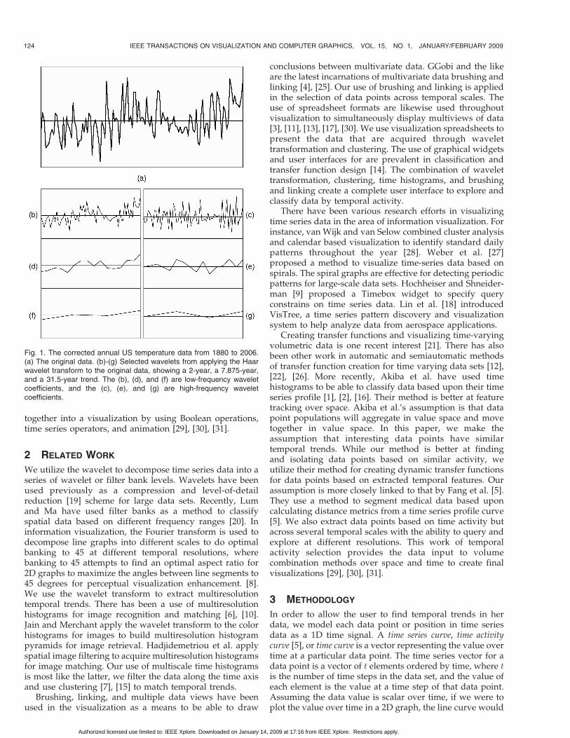
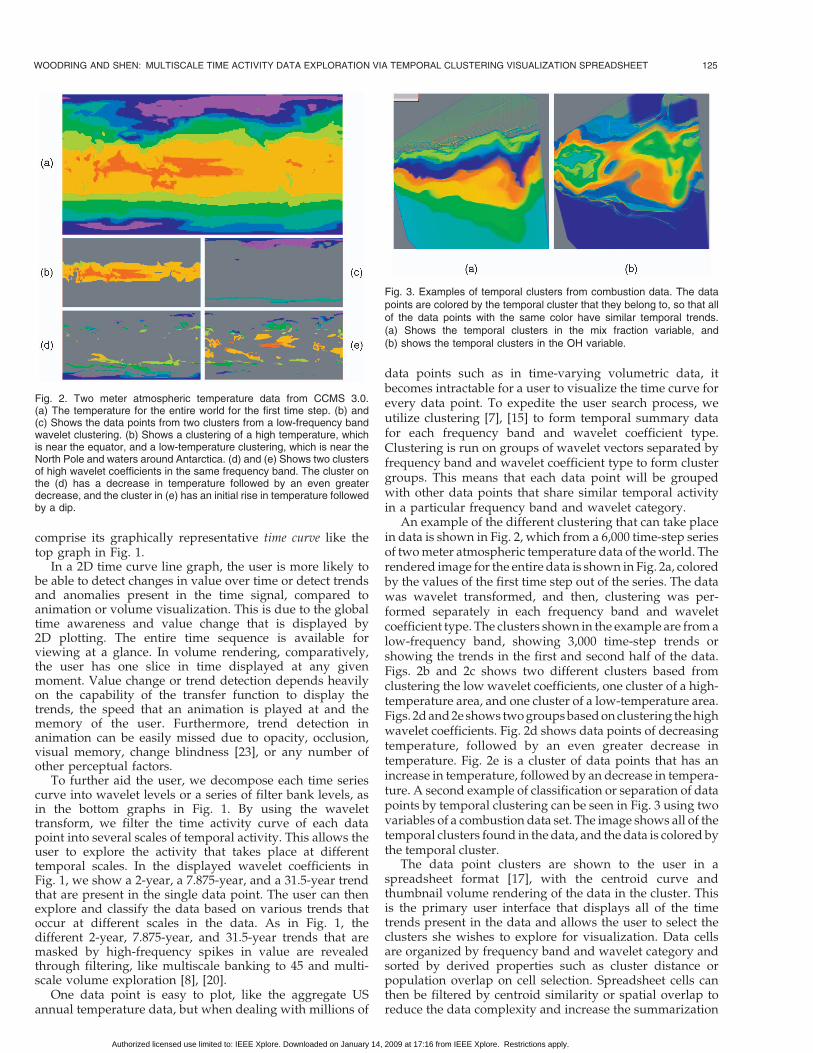
An example of the different clustering that can take placein data is shown in Fig. 2, which from a 6,000 time-step seriesof two meter atmospheric temperature data of the world. Therendered image for the entire data is shown in Fig. 2a, coloredby the values of the first time step out of the series. The datawas wavelet transformed, and then, clustering was per-formed separately in each frequency band and waveletcoefficient type. The clusters shown in the example are from alow-frequency band, showing 3,000 time-step trends orshowing the trends in the first and second half of the data.Figs. 2b and 2c shows two different clusters based fromclustering the low wavelet coefficients, one cluster of a high-temperature area, and one cluster of a low-temperature area.Figs. 2d and 2e shows two groups based on clustering the highwavelet coefficients. Fig. 2d shows data points of decreasingtemperature, followed by an even greater decrease intemperature. Fig. 2e is a cluster of data points that has anincrease in temperature, followed by an decrease in tempera-ture. A second example of classification or separation of datapoints by temporal clustering can be seen in Fig. 3 using twovariables of a combustion data set. The image shows all of thetemporal clusters found in the data, and the data is colored bythe temporal cluster.

The data point clusters are shown to the user in aspreadsheet format [17], with the centroid curve andthumbnail volume rendering of the data in the cluster. Thisis the primary user interface that displays all of the timetrends present in the data and allows the user to select theclusters she wishes to explore for visualization. Data cellsare organized by frequency band and wavelet category andsorted by derived properties such as cluster distance orpopulation overlap on cell selection. Spreadsheet cells canthen be filtered by centroid similarity or spatial overlap toreduce the data complexity and increase the summarization

WOODRING AND SHEN: MULTISCALE TIME ACTIVITY DATA EXPLORATION VIA TEMPORAL CLUSTERING VISUALIZATION SPREADSHEET 125

Fig. 2. Two meter atmospheric temperature data from CCMS 3.0.(a) The temperature for the entire world for the first time step. (b) and(c) Shows the data points from two clusters from a low-frequency bandwavelet clustering. (b) Shows a clustering of a high temperature, whichis near the equator, and a low-temperature clustering, which is near theNorth Pole and waters around Antarctica. (d) and (e) Shows two clustersof high wavelet coefficients in the same frequency band. The cluster onthe (d) has a decrease in temperature followed by an even greaterdecrease, and the cluster in (e) has an initial rise in temperature followedby a dip.

Fig. 3. Examples of temporal clusters from combustion data. The datapoints are colored by the temporal cluster that they belong to, so that allof the data points with the same color have similar temporal trends.(a) Shows the temporal clusters in the mix fraction variable, and(b) shows the temporal clusters in the OH variable.


of the time series data. A small spreadsheet is shown inFig. 4. This spreadsheet shows all of the low waveletcoefficient clusters in the frequency band that represents15.25 time-step trends for a 122 time-step data set.

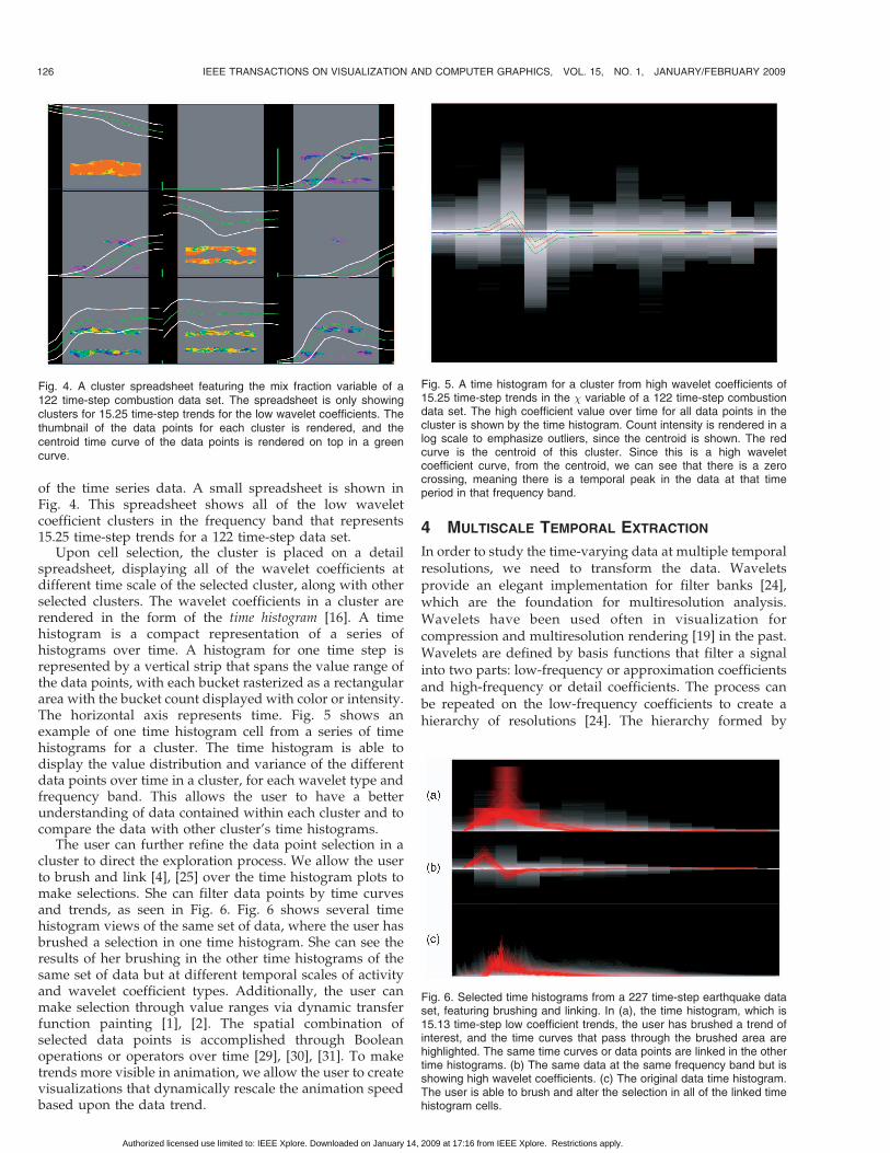
Upon cell selection, the cluster is placed on a detailspreadsheet, displaying all of the wavelet coefficients atdifferent time scale of the selected cluster, along with otherselected clusters. The wavelet coefficients in a cluster arerendered in the form of the time histogram [16]. A timehistogram is a compact representation of a series ofhistograms over time. A histogram for one time step isrepresented by a vertical strip that spans the value range ofthe data points, with each bucket rasterized as a rectangulararea with the bucket count displayed with color or intensity.The horizontal axis represents time. Fig. 5 shows anexample of one time histogram cell from a series of timehistograms for a cluster. The time histogram is able todisplay the value distribution and variance of the differentdata points over time in a cluster, for each wavelet type andfrequency band. This allows the user to have a betterunderstanding of data contained within each cluster and tocompare the data with other cluster’s time histograms.

The user can further refine the data point selection in acluster to direct the exploration process. We allow the userto brush and link [4], [25] over the time histogram plots tomake selections. She can filter data points by time curvesand trends, as seen in Fig. 6. Fig. 6 shows several timehistogram views of the same set of data, where the user hasbrushed a selection in one time histogram. She can see theresults of her brushing in the other time histograms of thesame set of data but at different temporal scales of activityand wavelet coefficient types. Additionally, the user canmake selection through value ranges via dynamic transferfunction painting [1], [2]. The spatial combination ofselected data points is accomplished through Booleanoperations or operators over time [29], [30], [31]. To maketrends more visible in animation, we allow the user to createvisualizations that dynamically rescale the animation speedbased upon the data trend.

4 MULTISCALE TEMPORAL EXTRACTION

In order to study the time-varying data at multiple temporalresolutions, we need to transform the data. Waveletsprovide an elegant implementation for filter banks [24],which are the foundation for multiresolution analysis.Wavelets have been used often in visualization forcompression and multiresolution rendering [19] in the past.Wavelets are defined by basis functions that filter a signalinto two parts: low-frequency or approximation coefficientsand high-frequency or detail coefficients. The process canbe repeated on the low-frequency coefficients to create ahierarchy of resolutions [24]. The hierarchy formed by


Fig. 4. A cluster spreadsheet featuring the mix fraction variable of a122 time-step combustion data set. The spreadsheet is only showingclusters for 15.25 time-step trends for the low wavelet coefficients. Thethumbnail of the data points for each cluster is rendered, and thecentroid time curve of the data points is rendered on top in a greencurve.

Fig. 5. A time histogram for a cluster from high wavelet coefficients of15.25 time-step trends in the � variable of a 122 time-step combustiondata set. The high coefficient value over time for all data points in thecluster is shown by the time histogram. Count intensity is rendered in alog scale to emphasize outliers, since the centroid is shown. The redcurve is the centroid of this cluster. Since this is a high waveletcoefficient curve, from the centroid, we can see that there is a zerocrossing, meaning there is a temporal peak in the data at that timeperiod in that frequency band.

Fig. 6. Selected time histograms from a 227 time-step earthquake dataset, featuring brushing and linking. In (a), the time histogram, which is15.13 time-step low coefficient trends, the user has brushed a trend ofinterest, and the time curves that pass through the brushed area arehighlighted. The same time curves or data points are linked in the othertime histograms. (b) The same data at the same frequency band but isshowing high wavelet coefficients. (c) The original data time histogram.The user is able to brush and alter the selection in all of the linked timehistogram cells.


repeated applications of the wavelet transform forms a filterbank or a set of band limited signals based upon the originalsignal. Among the different types of discrete wavelettransforms, the Haar wavelet and the Daubechies waveletare commonly used. The Haar wavelet is very fast tocalculate and has a simple support, and from the user pointof view, the calculation of the wavelet and its meaning issimple to understand. We have a series of increasingly low-pass signals based upon the original signal, representing thedata at different time scales. Also, we have the derivativesof each of the low-pass signals, showing the rate of changeof the data over different time scales.

4.1 Haar Wavelet

Assuming that the time sampling rate for the data is regularor can be converted to a uniform sampling rate, we use theHaar wavelet to transform the data into a multiscaletemporal format. The Haar wavelet has several differentnotational forms. The version that we use is the low-frequency coefficients being the mean of two adjacentsamples, and the high-frequency coefficients being thedifference of two adjacent samples. The reason for thisnotation and is for the ease of understanding from the userpoint of view, rather than reconstruction support. In thiswork, the wavelet transform is used to represent the timeseries at different temporal scales for user exploration. Byreasoning on the wavelet transform in this way, to the user,the low-frequency wavelet coefficients are the average orvalue signal, and the high-frequency wavelet coefficientsare the rate-of-change or derivative signal. The Haartransform is given in (1) and (2), where O is the originalsignal, L are the low-frequency coefficients, and H are thehigh-frequency coefficients:

Li ¼ ðO2iþ1 þO2iÞ=2; ð1Þ

Hi ¼ O2iþ1 �O2i: ð2Þ

The recursive process of applying the Haar transform onthe L coefficients results in a cascading filter bank ofdlog2ðtÞe levels of low-frequency coefficients and high-frequency coefficients, where t is the number of samples.For reconstruction, strictly speaking, a level l filter bank hasdt=2le low-frequency coefficients and dt=2le high-frequencycoefficients.

Though in our visualization, we use dt=2l�1 � 1e high-frequency coefficients to display the difference betweenevery adjacent time step. Strictly speaking, if we were usingthe wavelet as a compression or back-end level-of-detailmethod, the additional coefficients are extraneous forreconstruction. The additional coefficients are for visualiza-tion and user analysis to show the difference between everytime point. For example, given eight data points, 12233445,the strict Haar high-frequency coefficients would be 1111.Instead of visualizing those coefficients, we increase thenumber and show the user 1010101, which is much moreinformative in terms of showing the rate of change of thesignal. This is on the order of a 2ðnlognÞ transformation,because of the extra set of coefficients.

For our data transformation, for a data point x in a timevarying data set, it has t samples over time, where t is the

number of steps in the time series. The t samples of x form atime series vector v, where the elements of v are ordered bytime. The Haar transform is applied to every time vector inthe data set, such that for every v, HaarðvÞ is a Haar wavelethierarchy representing data point x at different frequencybands and wavelet coefficient types. Alternatively, it can bethought of as filtering a data point x across time to extractits characteristic signal across frequency bands and signaltypes. This wavelet transformation is used to display a datapoint’s temporal trend at various temporal scales to theuser. Assuming that the data is scalar, the multiscaletemporal trend of a data point can be displayed by drawingthe 2D curve of each wavelet vector.

Fig. 1 is an example of applying the Haar wavelettransform to one data point. Fig. 1a is the originaltemperature over time. Figs. 1b, 1c, 1d, 1e, 1f, and 1g arethe wavelet transformed data plots.

4.2 Temporal Activity Clustering

It is not possible to be able to draw every 2D wavelet graph forevery data point in a data set of realistic size. There would besimply be too many line graphs to plot and explore. In order toreduce the data set size and to create summary information,we employ clustering on the wavelet data. Clustering is amethod for grouping a set of high-dimensional vectors intosemantic sets. In the most general terms, a similarity ordistance metric is repeatedly applied to the input set ofvectors to separate the data into semantic groups or clusters.Common methods for clustering include energy minimiza-tion solutions like K-Means and machine learning algorithmslike the self-organizing map (SOM) [7], [15].

Our use of clustering is employed on the time vectorsthat are generated through the wavelet transform to formsets of data points that exhibit similar time activities. Foreach data point x in a time series data set, it will have2 � dlog2ðtÞe þ 1 vectors representing the original data andthe low-frequency and high-frequency wavelets from theHaar transform. For each of the vector types, we clusterthe data points in the time-varying data set. Since wehave 2 � dlog2ðtÞe þ 1 groups of frequency band and signaltype, a data point x will belong to one cluster in each ofthe groups as a result of this clustering process.

By performing clustering on each signal type separately,a data point is grouped with other data points that havesimilar temporal activity in a particular frequency band andwavelet type. By clustering by low coefficients, temporalactivity grouping is dominated by value over time. Whengrouping by high coefficients, data points are clustered bythe rate-of-change over time. This allows the user to explorethe range of possibilities of temporal trends over eachfrequency band and signal type. We assume that there willbe population separation in the clustering, such that clustersacross frequency bands and wavelet coefficient types willhave different data point populations. This is whereinteresting temporal trends should appear in exploration.

Fig. 2 displays several clusters in a low-frequency band.The second row shows data points that were groupedtogether because they had similar low wavelet coefficientactivity over time in that frequency band. If we cluster byhigh wavelet coefficients, we obtain clusters, seen inFigs. 2d and 2e, that contain some of the same data points



in the first two clusters. Therefore, the user can make a morerefined selection by taking the intersection, through Booleanoperations, between two clusters. For example, if the userintersects the cluster in Fig. 2b with the cluster in Fig. 2e, sheis able to visualize a region that not only has hightemperature value but also is raised and then dipped intemperature.

The clustering method that we use is a hybrid SOM and K-Means with kd-tree acceleration. While K-Means and kd-treeare well known, the SOM is an AI learning network thatprojects high-dimensional vectors to a lower dimensionalspace, while trying to preserve the topology of the higherdimension space. We use the SOM to quickly arrive at aninitial, hopefully globally optimal, centroid set for clusteringand then use K-Means to refine the set to a convergentanswer. The drawback is that the K-Means and SOM requirethe number of clusters as input; therefore, it may under orovercluster because the number of clusters picked may not bethe number of natural clusters in the data. The initial use ofSOM attempts to shake K-Means into a global minimumrather than a local minimum. There may be utility in using analternative clustering method for creating temporal summa-ries, compared to the clustering we have used.

One drawback or limitation that we have in our method isthat we are able to classify data points into temporal hotspotssuch as regions in space that share the same activity, but weare not able to do spatial tracking of values or temporal phaseshift. For example, in the case studies found later in the paper,our method is able to classify the weather data intogeographical regions by their temperature patterns overtime. Though, for data such as the combustion data set, weclassify volumetric regions that have spatially moving datavalues that are moving through a region, rather than trackingthe value over space. This is because a value moving throughspace appears as an impulse time curve as it passes throughdifferent regions of space.

5 USER INTERFACE

The goal of the user interface is to display the time activityof a data set and to allow the user to select data points basedon the visualized temporal activity. A cluster spreadsheet isformed from data acquired through wavelet transform andclustering on the input. From the clusters, the user is able toexplore and find data that have interesting temporalactivity. To get further detail, the user can select the clustersof interest and place them on a time histogram spreadsheet.From the cluster selection and refinement, the visualizationis formed, highlighting the data of user selected temporalactivity, which in turn can lead to further refinement andexploration.

5.1 Cluster Spreadsheet

The cluster spreadsheet is the primary interface that formsthe temporal trend exploration. Each cell of the spreadsheetrepresents a cluster formed from the clustering of waveletdata, explained in the previous sections. The cells are sortedby spreadsheet columns, such that each column containsclusters of one wavelet level (frequency band), and sortedleft to right by the lowest detail to the highest detail.

Low wavelet coefficients are on the left half of thespreadsheet, while high wavelet coefficients are on theright half of the spreadsheet, so that comparisons can bemade between wavelets of the same type. Given thatthere are dlog2ðtÞe wavelet levels (frequency bands) fromthe Haar wavelet transformation, two wavelet coefficienttypes from the low and high coefficients, and a fixednumber of clusters k per wavelet category type, thenthere will be 2 � dlog2ðtÞe � k cells in the spreadsheet,where there are k rows and 2 � dlog2ðtÞe columns. Anexample full cluster spreadsheet can be seen in Fig. 7.

To show the summary information, each cell graphs thecentroid time curve of the cluster, the average variance ofthe cluster members from the centroid, and a thumbnailrendering of the data points in the cluster, giving a temporaland spatial summary of the data that is contained in eachcluster, as seen in Fig. 8. On the right edge of the cell is a barindicating the ratio of population of data points in thecluster to the total data point population, so the user can seethe size of the cluster. Next to that, there is an additional barindicating either intersecting population count or centroiddistance from a reference cluster that is selected by the user.The quantity that this bar shows is used in relevancereorganization, as is explained below.

One point of mention is that this spreadsheet interfacecan have a problem with data explosion or overwhelmingthe user with too much information. Since we extractseveral different time scales and multiple clusters of data, itcan be a daunting task for the user to be able to search andexplore the data. The clustering was a first pass at datareduction, and we have several different user interfacecontrols sorting and simplify the amount of data shown tothe user. Our user interface makes a good attempt forvisualizing multiscale temporal data, but there is room forfuture improvement, beyond what we have done here.

5.2 Relevance Reorganization

When the user selects a particular cluster cell, the entirespreadsheet is reorganized to display the relative relevanceof other clusters to the selected cluster. The basic rules forreorganization is that a cell will stay in its own column, ascolumn is an indication of frequency band and waveletcoefficient type. A cell can move up or down within itscolumn. The goal of sorting in the column is to move cellsvertically closer to the picked cell so that closer cells willhave higher relevance. Therefore, when the user is brows-ing the spreadsheet, after choosing a cell, she is presentedwith a spatial reorganization of the spreadsheet to displayclusters with similar temporal or cluster populationcharacteristics. We note that all the following reorganizationmethods can be inverted to reorganize the cluster spread-sheet to highlight dissimilar cells when necessary.

5.2.1 Same Column Reorganization

Within the column that a picked cell resides, other cells inthat column are reorganized based on the cluster centroiddistance from the picked cell. The effect is that when a userpicks a cell, clusters in the same column are moved closer ifthey have a smaller distance using the clustering distancemetric between their temporal centroids and moved fartheraway if there is a larger distance. The first columns of the



images in Fig. 9 show an example of resorting cells in thecolumn of the picked cell. Cells that are temporally similarhave moved closer, in this case, similar cold temperatures tothe picked cell (please see the figure caption for detail). Bymoving cells that have similar centroids closer to a targetcluster, we emphasize the clusters that have the same

temporal trend as the picked cluster. In addition toresorting the cells, we always show the relative normalizedtemporal centroid distance in a cell with a red vertical baron the right of the cell.

5.2.2 Other Column Reorganization

The other columns, which are not the column of a pickedcell, are sets of clusters in different frequency bands andwavelet coefficient types. In order to show their relevance toa picked cell, we can re-sort the cells vertically such thattheir relative vertical distance from a picked cell is equal tothe percentage of shared population from the picked cell.This is equal to COCðA;BÞ ¼ jA

TBj=jAj, where A is the

picked cell, and B is the cell to be sorted, which we callcrossover count. The second and third columns in Fig. 9ashows an example of how other column reorganizationworks. The user has picked cell 1 with cold temperatures,and cells with the highest overlapping data point popula-tion in other columns are moved vertically closer. Clustercells with smaller crossover count will be moved relativelyfarther away from the center row. By moving cells with thehighest shared percentage population vertically closest to apicked cell, we emphasize how data point populationsrecluster across frequency bands and where temporaltrends diverge across frequency bands. In this example,we can see that there is a split in the cluster population aswe increase in the detail of temporal scales. For thisparticular data set, we can reason that this is due to the


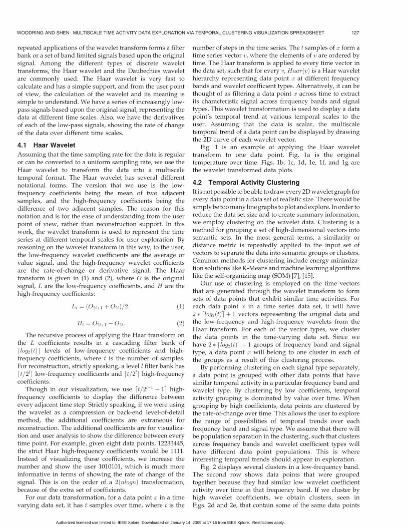
Fig. 7. A cluster spreadsheet of the OH variable of 122 time-step combustion data set. After the data has been wavelet transformed and clustered, itis organized into a spreadsheet. The left half of the spreadsheet shows low wavelet coefficients, while the right half shows high wavelet coefficients.The columns are organized from the lowest frequency band (long-term trends) to the highest frequency band (short-term trends), reading left to right.Each cell is one cluster of a particular frequency band and wavelet coefficient type. The spreadsheet gives a global view of the different trends thatare present in the time varying data.

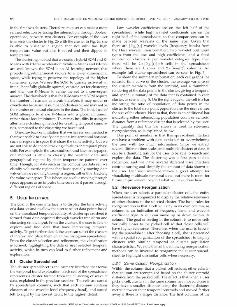
Fig. 8. A close up of a cluster cell from Fig. 7. The background of a cell (1)contains a thumbnail rendering of the data points in the cluster. In theforeground, the green curve (2) represents the centroid temporal trend ofthe data contained in the cluster. The white curves (3) indicate theaverage temporal variance around the centroid time curve. The green barin the lower right (4) indicates the population size of the cluster. Theyellow bar in the lower right (5) is for showing the data point overlap withanother cluster or the centroid distance from another cluster.


northern and southern hemisphere monthly temperature

cycle. In short term temporal trends, data points are

temporally similar to regions in the same hemisphere. In a

longer term trends, data points are similar to regions in the

same latitude, ignoring monthly trends. We always show

the crossover count between a picked cell and every other

cell by a yellow vertical bar on the right of a cell.

5.2.3 Row Sensitive Reorganization

To emphasize similarity across all rows, we can sort the

cells in each column based on a greedy crossover-count

selection compared with the cells in the column that the

picked cell resides. To do this, the picked cell first movesthe cell with the highest crossover count in each columnvertically into its row. Then, the cell with the smallestcentroid distance to the picked cell in the same column doesthe same, i.e., it moves the cell with the highest crossovercount with itself in each column vertically into its row. Thisis repeated for the next smallest centroid distance clusteruntil there are no more cells to reorganize. Fig. 9b shows anexample of using this reorganization method on thespreadsheet. Rows A and B are populationally similar tothe clusters 2 and 3, respectively, in the column where thepicked cell resides. This tries to ensure that there isrelevance across columns as well, such that the user readsacross rows, all of the clusters are from similar data pointpopulation, although this is not always guaranteed due tothe greedy selection method we use. We can see a shift inthe other cluster populations over temporal scales, as wellas the picked cell. The user can still see the crossover countwith the picked cell by the yellow bar on each other cell. Asan alternative for using crossover count as a reorganizationmetric, the centroid distance between clusters can be usedas well in the previous two methods for sorting columns toemphasize temporal trend similarity between clustersrather than population similarity.

5.3 Spreadsheet Simplification

The user interface visualization can be complex due to thefact that many cells are displayed at once, like in Fig. 7.Further simplification can be done by only showing a fewcolumns of interest, like we have done in Fig. 9. Alter-natively, we can use similarity metrics to automatically cullcells or reduce the number of cells. Clustering acrossdifferent frequency bands results in clusters with differentpopulations, but there will still be overlap in the populationof data points. Like in Fig. 9, there is a shift in clusterpopulation indicating a shift or change in temporal trends,but many of the clusters have similar populations acrosstemporal scales. By culling clusters that have similarpopulations but retaining ones with different populations,we reduce the complexity of the spreadsheet but preservethe information.

5.3.1 Cell Culling

After the user selects an initial set of clusters, instead ofshowing clusters thatmight be considered redundant becausethey have similar data point populations, cells can be culled ifthe cluster population does not exceed a percentage popula-tion difference threshold from the closest cluster populationin the selection set. This percentage population crossovercount is the maximum of the size of the intersection setbetween two clustersAandBdivided byA for allA in the userselection set U , MCOCðBÞ ¼ maxð8A 2 U : jA

TBj=jAjÞ.

This is performed incrementally in a greedy manner, addingnew cells to the user selection set U as they exceed thepopulation threshold. An example can be seen in Fig. 10. Cellculling tends to be able to discard low wavelet coefficientclusters, because clusters tend to be similar over temporalscales. On the other hand, high wavelet coefficients, by theirvery nature, retain the detail information of every temporalscale and thus are unlikely to carry the same clusterpopulation over temporal scales.


Fig. 9. Two sorted views of a portion of a cluster spreadsheet for 2-metermonthly temperature data of 6,000 time steps, showing clusters of datapoints that have similar (left to right) 32-month, 16-month, and 8-monthtrends. In (a), the user has picked cell 1. Cells in the same column aresorted by the centroid time curve distance to the selected cell, so thatclusters 2 and 3 of similar temperatures over time have moved closer tothe picked cell. This is also indicated by the length of the red bar in thecells. Cells in the other columns are sorted, such that cells that has agreater population overlap with cell 1 are moved vertically closer butstays in the same column. This can also be quantitatively seen by thelength of the yellow bar in the cells. In (b), the difference is that cells inrow A have the highest overlap with cell 2, and cells in row B have thehighest overlap with cell 3.


5.3.2 Cell Merging

Additionally, we can use the distance metric used in the

clustering algorithm to merge cells in the same column

based on the centroid difference. Cell merging is a type of

user based clustering to reduce the screen area occupied by

the spreadsheet. If two clusters have similar centroids, such

that the distance between two cluster centroids is under a

threshold, we merge the cells to an overlay cell. The user

can manually merge cells together to form a cell union if she

decides that the data is similar or belongs together. All of

the centroids merged together are rendered in the overlay

cell, and the rendered thumbnail of the clusters is a spatial

union of the combined cluster data. The user is allowed to

resplit the clusters into individual cells of their own, if she

only wishes to pick one cluster or to see the data of each

cluster individually.

5.4 Time Histogram Spreadsheet

When the user selects a cluster, it is added to a secondary

spreadsheet, a time histogram spreadsheet, as in Fig. 11. The

column layout is the same, such that there are two halves

corresponding to low and high wavelet coefficients, and

each column corresponds to one frequency band. Initially,

the time histogram spreadsheet is empty. When a cluster is

selected, it is added as a new row to the time histogram

spreadsheet, and the time histogram of the cluster across

frequency bands is displayed in each column for a row. Thetime histogram in each frequency band provides asummary of the time curves that are contained within acluster, so that the user can see the details of distribution ofvalues over time. If there is more than one row, thespreadsheet is resorted to show the relevance betweenclusters, as was mentioned in the previous section.Essentially, the time histogram spreadsheet is to displaydetails for the selected clusters. It also provides a good


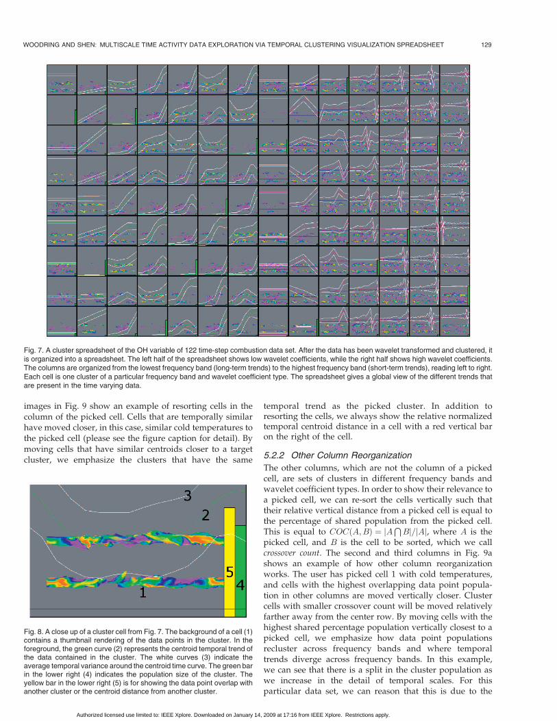
Fig. 10. An example of culled spreadsheet of � variable from 122 time-step combustion data set. The culling order was performed from the highest

detail to the lowest detail at a 75 percent population threshold. There were 35 cells that have been culled out of 126, resulting in a 27-percent space

savings. By culling cluster cells that do not change populations over temporal scales, the essence of the temporal trends in are retained and even

highlighted since they are the only cells that remain.

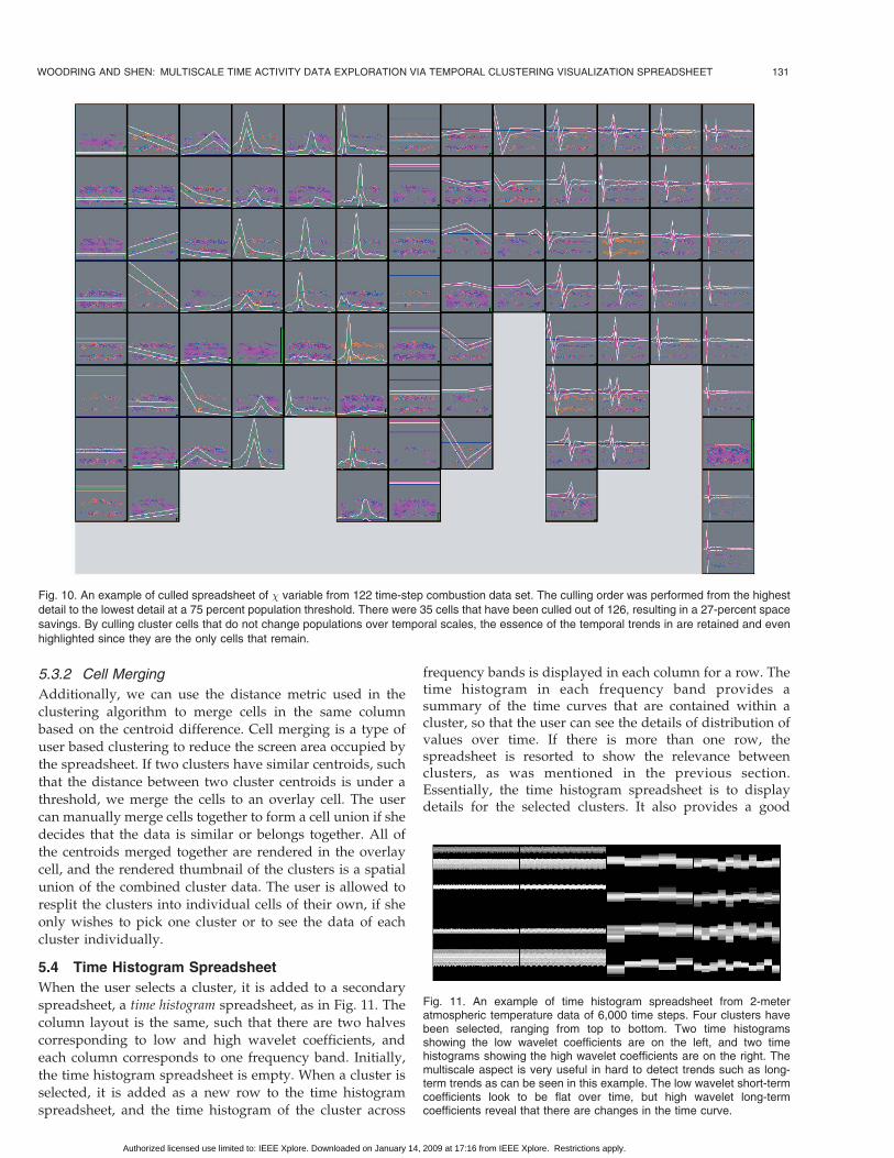
Fig. 11. An example of time histogram spreadsheet from 2-meteratmospheric temperature data of 6,000 time steps. Four clusters havebeen selected, ranging from top to bottom. Two time histogramsshowing the low wavelet coefficients are on the left, and two timehistograms showing the high wavelet coefficients are on the right. Themultiscale aspect is very useful in hard to detect trends such as long-term trends as can be seen in this example. The low wavelet short-termcoefficients look to be flat over time, but high wavelet long-termcoefficients reveal that there are changes in the time curve.


interface for the user to be able to make fine tuningadjustments of the data points within a cluster, as describedbelow.

5.4.1 Time Curve Brushing and Linking

Our manipulation of the data contained within a cluster is abrush widget. There are two modes of operation with thebrush widget. In the first mode, the user paints an area intime histogram she wants to explore, and time curves thatpass through the selected bucket on the time histogram areselected. Any time curves that fall within the user paintedarea are selected, drawn as polylines, and linked [4], [25]across the time histogram columns, seen in Fig. 6. Bydrawing the curves as continuous polyline rather thanplotting the data points, the change in value over timebecomes more apparent. The user can make refinedselections by using intersection, union, and differencebrushes, such that the different brushes remove or adddata points from the selection set based on the operation ofa brush. By linking time curves across frequency bands, theuser can see the temporal profile of the data and potentiallymake fine tuning adjustments in another frequency space.Brushing and linking is restricted to the data within acluster or a merged cluster. To make clear the relationshipsbetween clusters, the user can use spatial Boolean operatorsto combine clusters into one visualization.

5.4.2 Dynamic Transfer Function Brushing and Linking

The second mode of operation uses value space selection[1], [2], rather than time curve selection. By painting on thetime histogram with color and opacity brushes, the user cancreate a temporally dynamic transfer function. She paintsthe value of the transfer function over time by using thetime histogram as a guide for value ranges. The paint islinked across all time histograms within a row, such that ifthe user paints in another frequency band, the transferfunction is updated. The paint can also be linked acrossrows, such that the transfer function can be shared acrossseveral clusters.

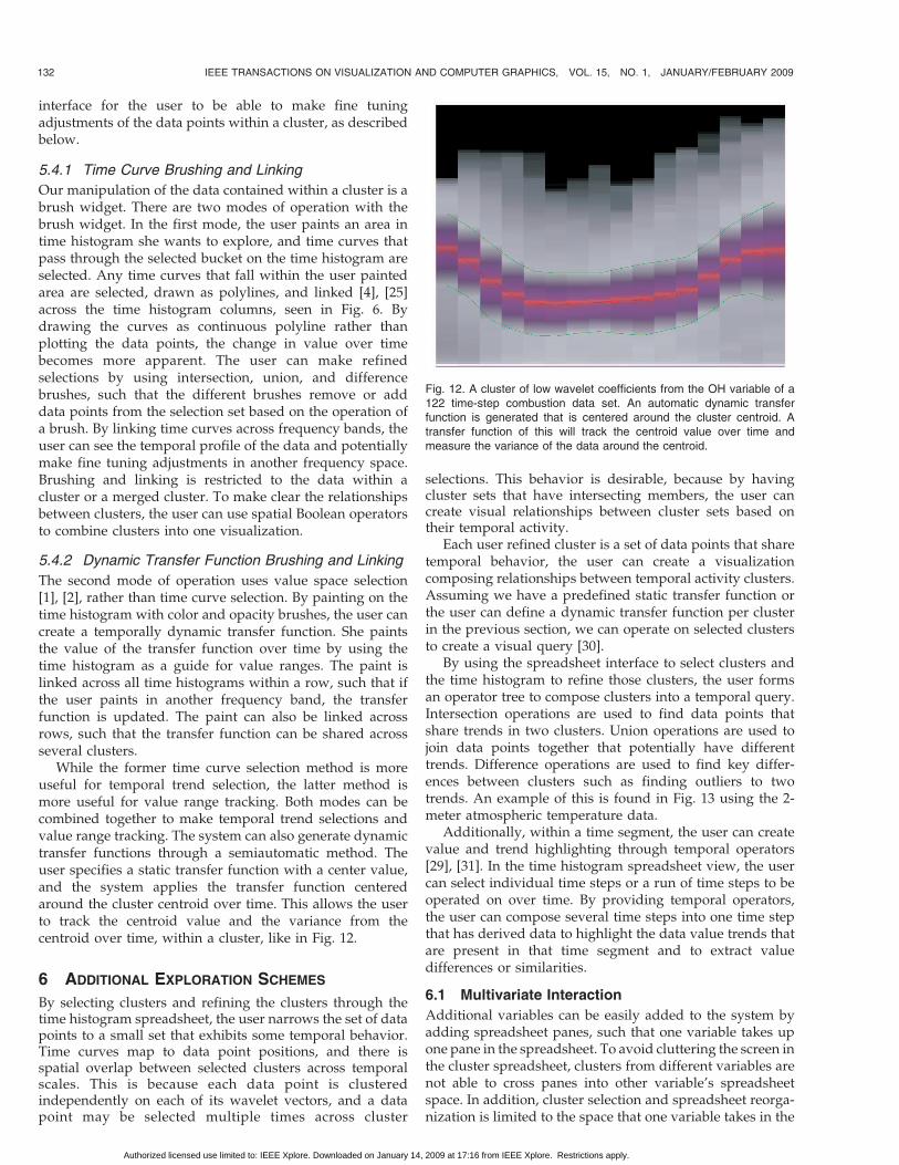
While the former time curve selection method is moreuseful for temporal trend selection, the latter method ismore useful for value range tracking. Both modes can becombined together to make temporal trend selections andvalue range tracking. The system can also generate dynamictransfer functions through a semiautomatic method. Theuser specifies a static transfer function with a center value,and the system applies the transfer function centeredaround the cluster centroid over time. This allows the userto track the centroid value and the variance from thecentroid over time, within a cluster, like in Fig. 12.

6 ADDITIONAL EXPLORATION SCHEMES

By selecting clusters and refining the clusters through thetime histogram spreadsheet, the user narrows the set of datapoints to a small set that exhibits some temporal behavior.Time curves map to data point positions, and there isspatial overlap between selected clusters across temporalscales. This is because each data point is clusteredindependently on each of its wavelet vectors, and a datapoint may be selected multiple times across cluster

selections. This behavior is desirable, because by havingcluster sets that have intersecting members, the user cancreate visual relationships between cluster sets based ontheir temporal activity.

Each user refined cluster is a set of data points that sharetemporal behavior, the user can create a visualizationcomposing relationships between temporal activity clusters.Assuming we have a predefined static transfer function orthe user can define a dynamic transfer function per clusterin the previous section, we can operate on selected clustersto create a visual query [30].

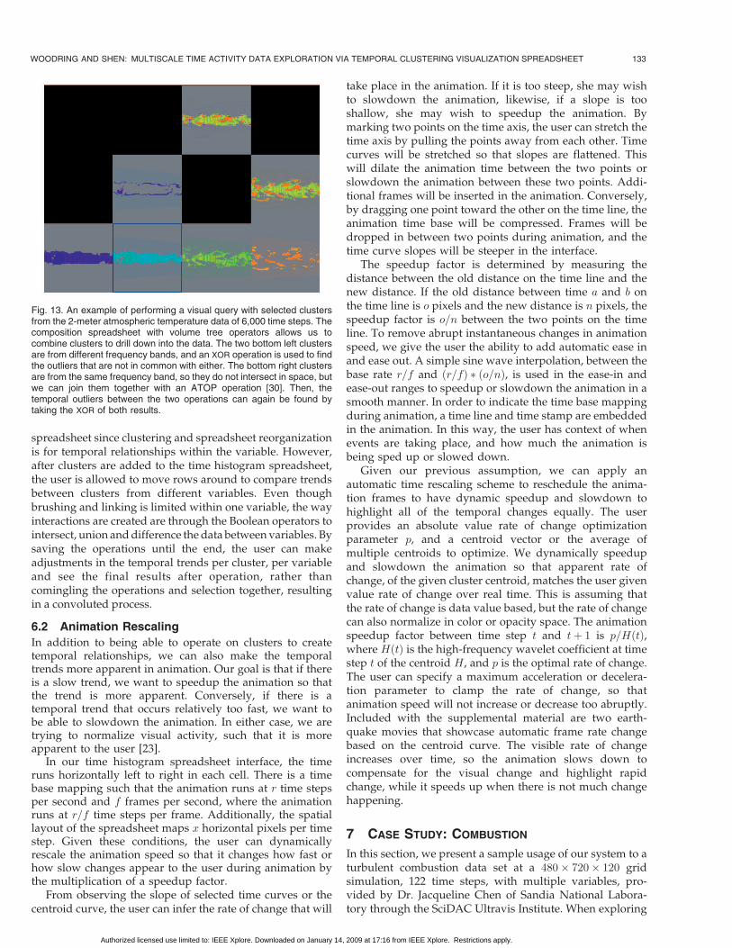
By using the spreadsheet interface to select clusters andthe time histogram to refine those clusters, the user formsan operator tree to compose clusters into a temporal query.Intersection operations are used to find data points thatshare trends in two clusters. Union operations are used tojoin data points together that potentially have differenttrends. Difference operations are used to find key differ-ences between clusters such as finding outliers to twotrends. An example of this is found in Fig. 13 using the 2-meter atmospheric temperature data.

Additionally, within a time segment, the user can createvalue and trend highlighting through temporal operators[29], [31]. In the time histogram spreadsheet view, the usercan select individual time steps or a run of time steps to beoperated on over time. By providing temporal operators,the user can compose several time steps into one time stepthat has derived data to highlight the data value trends thatare present in that time segment and to extract valuedifferences or similarities.

6.1 Multivariate Interaction

Additional variables can be easily added to the system byadding spreadsheet panes, such that one variable takes upone pane in the spreadsheet. To avoid cluttering the screen inthe cluster spreadsheet, clusters from different variables arenot able to cross panes into other variable’s spreadsheetspace. In addition, cluster selection and spreadsheet reorga-nization is limited to the space that one variable takes in the


Fig. 12. A cluster of low wavelet coefficients from the OH variable of a122 time-step combustion data set. An automatic dynamic transferfunction is generated that is centered around the cluster centroid. Atransfer function of this will track the centroid value over time andmeasure the variance of the data around the centroid.


spreadsheet since clustering and spreadsheet reorganizationis for temporal relationships within the variable. However,after clusters are added to the time histogram spreadsheet,the user is allowed to move rows around to compare trendsbetween clusters from different variables. Even thoughbrushing and linking is limited within one variable, the wayinteractions are created are through the Boolean operators tointersect, union and difference the data between variables. Bysaving the operations until the end, the user can makeadjustments in the temporal trends per cluster, per variableand see the final results after operation, rather thancomingling the operations and selection together, resultingin a convoluted process.

6.2 Animation Rescaling

In addition to being able to operate on clusters to createtemporal relationships, we can also make the temporaltrends more apparent in animation. Our goal is that if thereis a slow trend, we want to speedup the animation so thatthe trend is more apparent. Conversely, if there is atemporal trend that occurs relatively too fast, we want tobe able to slowdown the animation. In either case, we aretrying to normalize visual activity, such that it is moreapparent to the user [23].

In our time histogram spreadsheet interface, the timeruns horizontally left to right in each cell. There is a timebase mapping such that the animation runs at r time stepsper second and f frames per second, where the animationruns at r=f time steps per frame. Additionally, the spatiallayout of the spreadsheet maps x horizontal pixels per timestep. Given these conditions, the user can dynamicallyrescale the animation speed so that it changes how fast orhow slow changes appear to the user during animation bythe multiplication of a speedup factor.

From observing the slope of selected time curves or thecentroid curve, the user can infer the rate of change that will

take place in the animation. If it is too steep, she may wishto slowdown the animation, likewise, if a slope is tooshallow, she may wish to speedup the animation. Bymarking two points on the time axis, the user can stretch thetime axis by pulling the points away from each other. Timecurves will be stretched so that slopes are flattened. Thiswill dilate the animation time between the two points orslowdown the animation between these two points. Addi-tional frames will be inserted in the animation. Conversely,by dragging one point toward the other on the time line, theanimation time base will be compressed. Frames will bedropped in between two points during animation, and thetime curve slopes will be steeper in the interface.

The speedup factor is determined by measuring thedistance between the old distance on the time line and thenew distance. If the old distance between time a and b onthe time line is o pixels and the new distance is n pixels, thespeedup factor is o=n between the two points on the timeline. To remove abrupt instantaneous changes in animationspeed, we give the user the ability to add automatic ease inand ease out. A simple sine wave interpolation, between thebase rate r=f and ðr=fÞ � ðo=nÞ, is used in the ease-in andease-out ranges to speedup or slowdown the animation in asmooth manner. In order to indicate the time base mappingduring animation, a time line and time stamp are embeddedin the animation. In this way, the user has context of whenevents are taking place, and how much the animation isbeing sped up or slowed down.

Given our previous assumption, we can apply anautomatic time rescaling scheme to reschedule the anima-tion frames to have dynamic speedup and slowdown tohighlight all of the temporal changes equally. The userprovides an absolute value rate of change optimizationparameter p, and a centroid vector or the average ofmultiple centroids to optimize. We dynamically speedupand slowdown the animation so that apparent rate ofchange, of the given cluster centroid, matches the user givenvalue rate of change over real time. This is assuming thatthe rate of change is data value based, but the rate of changecan also normalize in color or opacity space. The animationspeedup factor between time step t and tþ 1 is p=HðtÞ,where HðtÞ is the high-frequency wavelet coefficient at timestep t of the centroid H, and p is the optimal rate of change.The user can specify a maximum acceleration or decelera-tion parameter to clamp the rate of change, so thatanimation speed will not increase or decrease too abruptly.Included with the supplemental material are two earth-quake movies that showcase automatic frame rate changebased on the centroid curve. The visible rate of changeincreases over time, so the animation slows down tocompensate for the visual change and highlight rapidchange, while it speeds up when there is not much changehappening.

7 CASE STUDY: COMBUSTION

In this section, we present a sample usage of our system to aturbulent combustion data set at a 480� 720� 120 gridsimulation, 122 time steps, with multiple variables, pro-vided by Dr. Jacqueline Chen of Sandia National Labora-tory through the SciDAC Ultravis Institute. When exploring


Fig. 13. An example of performing a visual query with selected clustersfrom the 2-meter atmospheric temperature data of 6,000 time steps. Thecomposition spreadsheet with volume tree operators allows us tocombine clusters to drill down into the data. The two bottom left clustersare from different frequency bands, and an XOR operation is used to findthe outliers that are not in common with either. The bottom right clustersare from the same frequency band, so they do not intersect in space, butwe can join them together with an ATOP operation [30]. Then, thetemporal outliers between the two operations can again be found bytaking the XOR of both results.


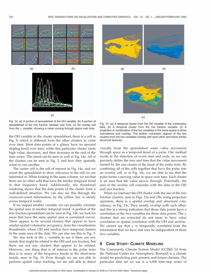
the OH variable in the cluster spreadsheet, there is a cell inFig. 8, which is different from the other clusters in valueover time. Most data points at a glance have an upwardsloping trend over time, while this particular cluster startshigh value, decreases, and then increases at the end of thetime series. This trend can be seen as well in Fig. 14a. All ofthe clusters can be seen in Fig. 3, and how they spatiallyrelate to one another.

The center cell is the cell of interest in Fig. 14a, and weresort the spreadsheet to show relevance to the cell we areinterested in. When looking in the same column, we see thatthere are no other cells that have the similar temporal trendin that frequency band. Additionally, the thumbnailrendering shows that the data points of the cluster form awell-defined structure. We can also see this through thecrossover-count information, by the yellow bar, is steadyacross temporal scales.

If we inspect another variable, we can possibly correlatethe spatial area to another temporal trend. A portion of themix fraction spreadsheet can be seen in Fig. 14b, we look forareas that have the same spatial area or correlated curves.There appear to be several clusters that appear to havesimilar spatial volumetric occupancy, from the visualizationthumbnails, where OH and mixfrac have temporal clustersin the same area of the data. We can also see this in Fig. 3.

We also look at the � variable to see if there are anytrends that might be related to the OH and mix fraction, butthere are not any clusters that appear to be related.However, one thing that is of interest is the pulse trainthat is in many of the frequency bands in the short-termtrends, seen in Fig. 10. Even though we are not able toperform spatial value tracking, we are still able to detect

visually from the spreadsheet some value movementthrough space as a temporal trend of a pulse. Our methodexcels at the detection of event start and ends, so we canprecisely define the area and time that the value movementstarted by the one cluster at the head of the pulse train. Bycombining all of the cells together that have the pulse intoan overlay cell, as in Fig. 14c, we are able to see that thepulse forms a moving value in space over time. Each clusteris an area that the value moves through. Potentially, thearea of the overlay cell coincides with the data in the OHand mix fraction.

When we intersect the OH cluster with the one of the mixfraction clusters, seen in Figs. 15a and 15b, using projectionoperators, there is a spatial overlap and structural coin-cidence, in Fig. 15c. They mostly overlap with each other,and this is a strong indication that those data points have acorrelation in the two variables for those data points. The �clusters that are extracted do not seem to have valuecorrelation or spatial correlation with the OH and mixfrac.We cannot say that � is temporally correlated from theinformation that we have and may be independent of thosetwo variables.

8 CASE STUDY: CLIMATE MODELING

The Community Climate System Model (CCSM) 3.0 fromthe National Center for Atmospheric Research is a climatemodel for predicting past, present, and future climates. Theparticular data set we use is a 6,000 time-step series of


Fig. 14. (a) A portion of spreadsheet of the OH variable. (b) A portion of

spreadsheet of the mix fraction variable over time. (c) An overlay cell

from the � variable, showing a value moving through space over time.

Fig. 15. (a) A temporal cluster from the OH variable of the combustiondata. (b) A temporal cluster from the mix fraction variable. (c) Aprojection or combination of the two variables in the same space to showcoincidence and overlap. The bottom volumetric regions of the twoclusters from the two variables overlap with each other and share similarstructural features.


world wide 2-meter monthly atmospheric temperature on a

256 � 128 2D grid. This multiscale temporal methodology

works quite well with climate model data and, in particular,

for the large number of time steps in the CCSM. By using

the multiresolution wavelets to filter time, we can see long-

term trends that might otherwise be obscured. The high

wavelet coefficients are well suited to show the activity that

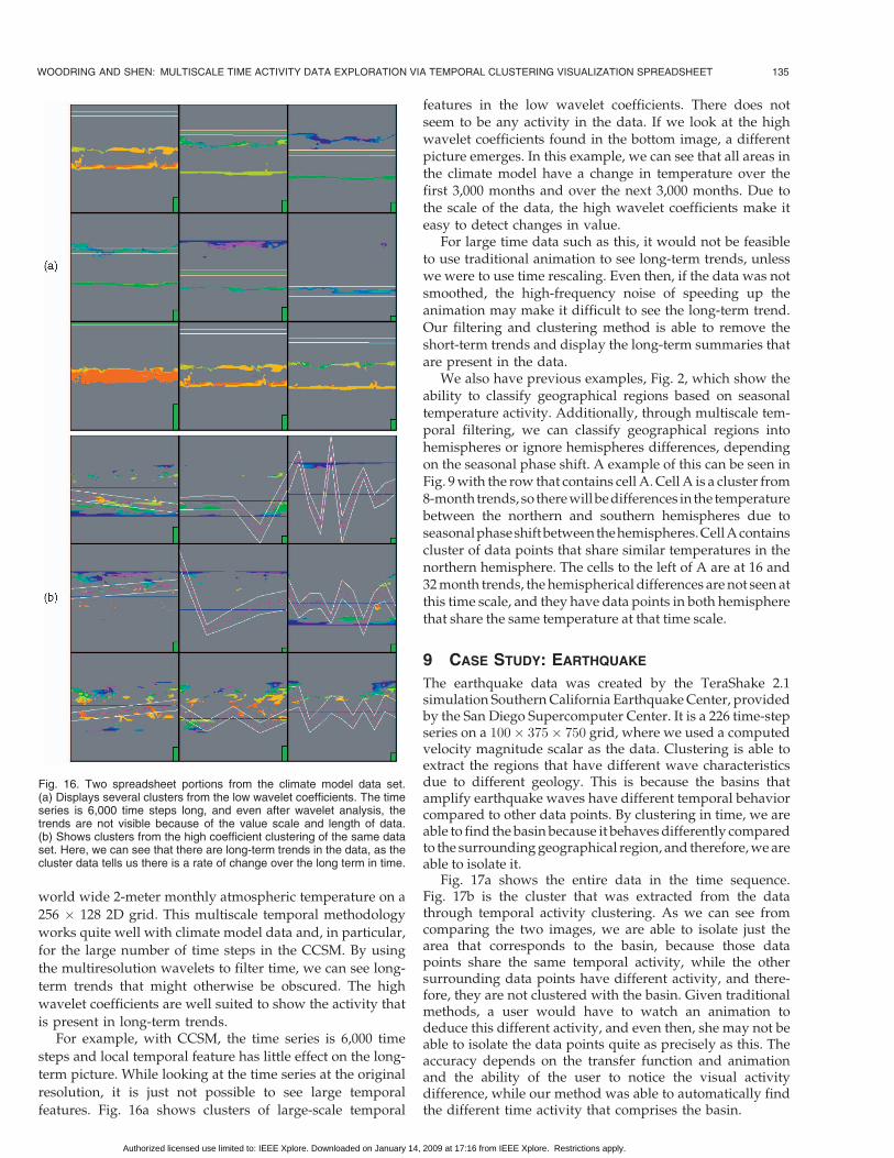
is present in long-term trends.For example, with CCSM, the time series is 6,000 time

steps and local temporal feature has little effect on the long-

term picture. While looking at the time series at the original

resolution, it is just not possible to see large temporal

features. Fig. 16a shows clusters of large-scale temporal

features in the low wavelet coefficients. There does notseem to be any activity in the data. If we look at the highwavelet coefficients found in the bottom image, a differentpicture emerges. In this example, we can see that all areas inthe climate model have a change in temperature over thefirst 3,000 months and over the next 3,000 months. Due tothe scale of the data, the high wavelet coefficients make iteasy to detect changes in value.

For large time data such as this, it would not be feasibleto use traditional animation to see long-term trends, unlesswe were to use time rescaling. Even then, if the data was notsmoothed, the high-frequency noise of speeding up theanimation may make it difficult to see the long-term trend.Our filtering and clustering method is able to remove theshort-term trends and display the long-term summaries thatare present in the data.

We also have previous examples, Fig. 2, which show theability to classify geographical regions based on seasonaltemperature activity. Additionally, through multiscale tem-poral filtering, we can classify geographical regions intohemispheres or ignore hemispheres differences, dependingon the seasonal phase shift. A example of this can be seen inFig. 9 with the row that contains cell A. Cell A is a cluster from8-month trends, so there will be differences in the temperaturebetween the northern and southern hemispheres due toseasonalphaseshift betweenthehemispheres. CellAcontainscluster of data points that share similar temperatures in thenorthern hemisphere. The cells to the left of A are at 16 and32 month trends, the hemispherical differences are not seen atthis time scale, and they have data points in both hemispherethat share the same temperature at that time scale.

9 CASE STUDY: EARTHQUAKE

The earthquake data was created by the TeraShake 2.1simulation Southern California Earthquake Center, providedby the San Diego Supercomputer Center. It is a 226 time-stepseries on a 100� 375� 750 grid, where we used a computedvelocity magnitude scalar as the data. Clustering is able toextract the regions that have different wave characteristicsdue to different geology. This is because the basins thatamplify earthquake waves have different temporal behaviorcompared to other data points. By clustering in time, we areable to find the basin because it behaves differently comparedto the surrounding geographical region, and therefore, we areable to isolate it.

Fig. 17a shows the entire data in the time sequence.Fig. 17b is the cluster that was extracted from the datathrough temporal activity clustering. As we can see fromcomparing the two images, we are able to isolate just thearea that corresponds to the basin, because those datapoints share the same temporal activity, while the othersurrounding data points have different activity, and there-fore, they are not clustered with the basin. Given traditionalmethods, a user would have to watch an animation todeduce this different activity, and even then, she may not beable to isolate the data points quite as precisely as this. Theaccuracy depends on the transfer function and animationand the ability of the user to notice the visual activitydifference, while our method was able to automatically findthe different time activity that comprises the basin.


Fig. 16. Two spreadsheet portions from the climate model data set.(a) Displays several clusters from the low wavelet coefficients. The timeseries is 6,000 time steps long, and even after wavelet analysis, thetrends are not visible because of the value scale and length of data.(b) Shows clusters from the high coefficient clustering of the same dataset. Here, we can see that there are long-term trends in the data, as thecluster data tells us there is a rate of change over the long term in time.


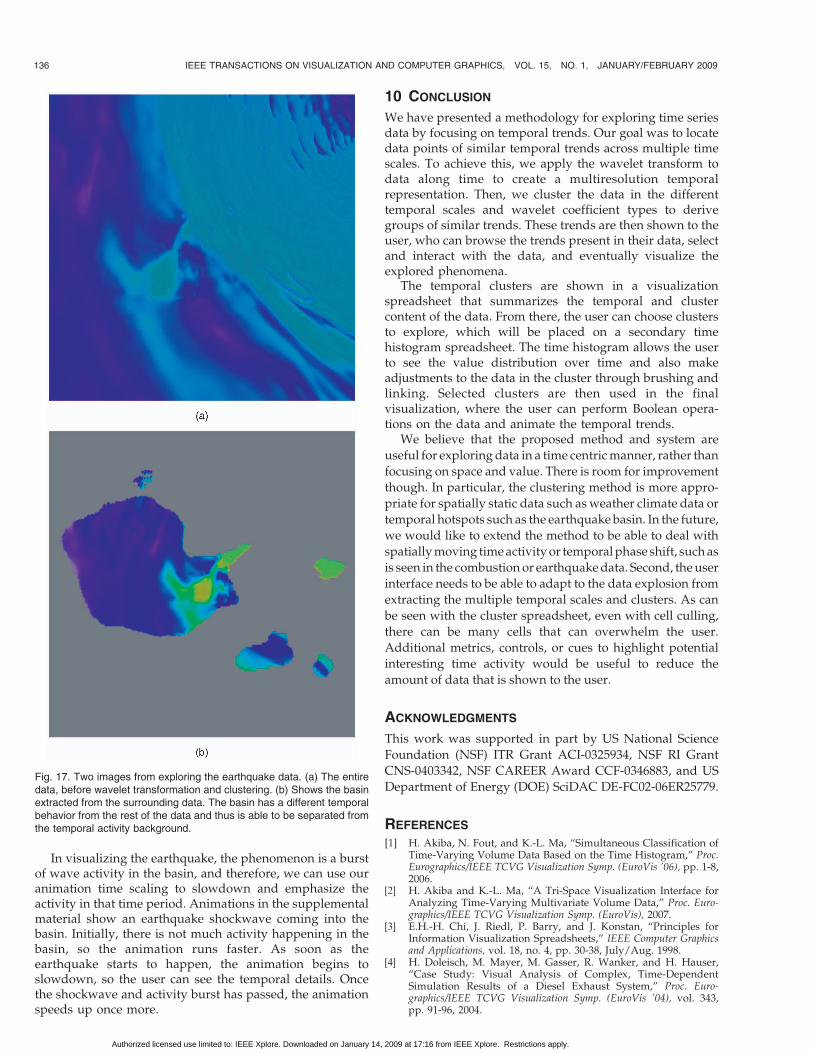
In visualizing the earthquake, the phenomenon is a burstof wave activity in the basin, and therefore, we can use ouranimation time scaling to slowdown and emphasize theactivity in that time period. Animations in the supplementalmaterial show an earthquake shockwave coming into thebasin. Initially, there is not much activity happening in thebasin, so the animation runs faster. As soon as theearthquake starts to happen, the animation begins toslowdown, so the user can see the temporal details. Oncethe shockwave and activity burst has passed, the animationspeeds up once more.

10 CONCLUSION

We have presented a methodology for exploring time seriesdata by focusing on temporal trends. Our goal was to locatedata points of similar temporal trends across multiple timescales. To achieve this, we apply the wavelet transform todata along time to create a multiresolution temporalrepresentation. Then, we cluster the data in the differenttemporal scales and wavelet coefficient types to derivegroups of similar trends. These trends are then shown to theuser, who can browse the trends present in their data, selectand interact with the data, and eventually visualize theexplored phenomena.

The temporal clusters are shown in a visualizationspreadsheet that summarizes the temporal and clustercontent of the data. From there, the user can choose clustersto explore, which will be placed on a secondary timehistogram spreadsheet. The time histogram allows the userto see the value distribution over time and also makeadjustments to the data in the cluster through brushing andlinking. Selected clusters are then used in the finalvisualization, where the user can perform Boolean opera-tions on the data and animate the temporal trends.

We believe that the proposed method and system are

useful for exploring data in a time centric manner, rather than

focusing on space and value. There is room for improvement

though. In particular, the clustering method is more appro-

priate for spatially static data such as weather climate data or

temporal hotspots such as the earthquake basin. In the future,

we would like to extend the method to be able to deal with

spatially moving time activity or temporal phase shift, such as

is seen in the combustion or earthquake data. Second, the user

interface needs to be able to adapt to the data explosion from

extracting the multiple temporal scales and clusters. As can

be seen with the cluster spreadsheet, even with cell culling,

there can be many cells that can overwhelm the user.

Additional metrics, controls, or cues to highlight potential

interesting time activity would be useful to reduce the

amount of data that is shown to the user.

ACKNOWLEDGMENTS

This work was supported in part by US National Science

Foundation (NSF) ITR Grant ACI-0325934, NSF RI Grant

CNS-0403342, NSF CAREER Award CCF-0346883, and US

Department of Energy (DOE) SciDAC DE-FC02-06ER25779.

REFERENCES

[1] H. Akiba, N. Fout, and K.-L. Ma, “Simultaneous Classification ofTime-Varying Volume Data Based on the Time Histogram,” Proc.Eurographics/IEEE TCVG Visualization Symp. (EuroVis ’06), pp. 1-8,2006.

[2] H. Akiba and K.-L. Ma, “A Tri-Space Visualization Interface forAnalyzing Time-Varying Multivariate Volume Data,” Proc. Euro-graphics/IEEE TCVG Visualization Symp. (EuroVis), 2007.

[3] E.H.-H. Chi, J. Riedl, P. Barry, and J. Konstan, “Principles forInformation Visualization Spreadsheets,” IEEE Computer Graphicsand Applications, vol. 18, no. 4, pp. 30-38, July/Aug. 1998.

[4] H. Doleisch, M. Mayer, M. Gasser, R. Wanker, and H. Hauser,“Case Study: Visual Analysis of Complex, Time-DependentSimulation Results of a Diesel Exhaust System,” Proc. Euro-graphics/IEEE TCVG Visualization Symp. (EuroVis ’04), vol. 343,pp. 91-96, 2004.


Fig. 17. Two images from exploring the earthquake data. (a) The entiredata, before wavelet transformation and clustering. (b) Shows the basinextracted from the surrounding data. The basin has a different temporalbehavior from the rest of the data and thus is able to be separated fromthe temporal activity background.


[5] Z. Fang, T. Moller, G. Harmarneh, and A. Celler, “Visualizationand Exploration of Spatio-Temporal Medical Image Data Sets,”Proc. Graphics Interface (GI ’07), pp. 281-288, 2007.

[6] E. Hadjidemetriou, M.D. Grossberg, and S.K. Nayar, “Multi-resolution Histograms and Their Use for Recognition,” IEEETrans. Pattern Analysis and Machine Intelligence, vol. 26, no. 7,pp. 831-847, July 2004.

[7] J.A. Hartigan and M.A. Wong, “Algorithm as 136: A k-MeansClustering Algorithm,” Applied Statistics, vol. 28, no. 1, pp. 100-108, 1979.

[8] J. Heer and M. Agrawala, “Multi-Scale Banking to 45 Degrees,”IEEE Trans. Visualization and Computer Graphics, vol. 12, no. 5,pp. 701-708, Sept./Oct. 2006.

[9] H. Hochheiser and B. Shneiderman, “Dynamic Query Tools forTime Series Data Sets: Timebox Widgets for Interactive Explora-tion,” IEEE Information Visualization, vol. 3, no. 1, pp. 1-8, 2004.

[10] P. Jain and S.N. Merchant, “Wavelet Based MultiresolutionHistogram for Fast Image Retrieval,” Proc. Conf. ConvergentTechnologies for Asia-Pacific Region (TENCON ’03), vol. 2, pp. 581-585, 2003.

[11] T. Jankun-Kelly and K.-L. Ma, “A Spreadsheet Interface forVisualization Exploration,” Proc. IEEE Visualization (VIS ’00),pp. 69-76, 2000.

[12] T. Jankun-Kelly and K.-L. Ma, “Study of Transfer FunctionGeneration for Time-Varying Volume Data,” Proc. Eurographics/IEEE TCVG Volume Graphics 2001, pp. 51-65, 2001.

[13] T. Jankun-Kelly and K.-L. Ma, “Visualization Exploration andEncapsulation via a Spreadsheet-Like Interface,” IEEE Trans.Visualization and Computer Graphics, vol. 7, no. 3, pp. 275-287,July-Sept. 2001.

[14] J. Kniss, G. Kindlmann, and C. Hansen, “Interactive VolumeRendering Using Multi-Dimensional Transfer Functions andDirect Manipulation Widgets,” Proc. IEEE Visualization (VIS ’01),pp. 255-562, 2001.

[15] T. Kohonen, Self Organizing Maps. Springer, 2001.[16] R. Kosara, F. Bendix, and H. Hauser, “Timehistograms for Large,

Time-Dependent Data,” Proc. Eurographics/IEEE TCVG Visualiza-tion Symp. (EuroVis ’04), vol. 340, pp. 45-54, 2004.

[17] M. Levoy, “Spreadsheets for Images,” Proc. ACM SIGGRAPH ’94,pp. 139-146, 1994.

[18] J. Lin, E. Koegh, S. Lonardi, J. Lankford, and D. Nystrom,“Visually Mining and Monitoring Massive Time Series,” Proc.ACM SIGKDD ’04, pp. 460-469, 2004.

[19] L. Linsen, V. Pascucci, M.A. Duchaineau, B. Hamann, and K.I. Joy,“Hierarchical Representation of Time-Varying Volume Data with“4th-Root-of-2” Subdivision and Quadrilinear B-Spline Wavelets,”Proc. Pacific Conf. Computer Graphics and Applications (PG ’02),pp. 346-355, 2002.

[20] E. Lum, J. Shearer, and K.-L. Ma, “Interactive Multi-ScaleExploration for Volume Classification,” Proc. Pacific Conf. Compu-ter Graphics and Applications (PG ’06), pp. 622-630, 2006.

[21] K.-L. Ma, “Visualizing Time-Varying Volume Data,” Computing inScience and Eng., vol. 5, no. 2, pp. 34-42, 2003.

[22] B. Petersch, M. Hadwiger, H. Hauser, and D. Honigmann, “RealTime Computation and Temporal Coherence of Opacity TransferFunctions for Direct Volume Rendering of Ultrasound Data,”Computerized Medical Imaging and Graphics, vol. 29, no. 1, pp. 53-63,2005.

[23] D.J. Simons and M.S. Ambinder, “Change Blindness: Theory andConsequences,” Current Directions in Psychological Science, vol. 14,no. 1, pp. 44-48, 2005.

[24] G. Strang and T. Nguyen, Wavelets and Filter Banks, first ed.Wellesley-Cambridge Press, 1996.

[25] D. Swayne, D.T. Lang, A. Buja, and D. Cook, “GGobi: Evolvingfrom XGobi into an Extensible Framework for Interactive DataVisualization,” Computational Statistics and Data Analysis, vol. 43,no. 4, pp. 423-444, 2003.

[26] F.-Y. Tzeng and K.-L. Ma, “Intelligent Feature Extraction andTracking for Visualizing Large-Scale 4D Flow Simulations,” Proc.ACM/IEEE Supercomputing (SC ’05), p. 6, 2005.

[27] M. Weber, M. Alexa, and W. Muller, “Visualizing Time-Series onSpirals,” Proc. IEEE Information Visualization (InfoVis ’01), pp. 7-14,2001.

[28] J.J.v. Wijk and E.R.v. Selow, “Cluster and Calendar BasedVisualization of Time Series Data,” Proc. IEEE InformationVisualization (InfoVis ’99), pp. 4-9, 1999.

[29] J. Woodring and H.-W. Shen, “Chronovolumes: A Direct Render-ing Technique for Visualizing Time-Varying Data,” Proc. Euro-graphics/IEEE TCVG Volume Graphics 2003, pp. 27-34, 2003.

[30] J. Woodring and H.-W. Shen, “Multi-Variate, Time Varying, andComparative Visualization with Contextual Cues,” IEEE Trans.Visualization and Computer Graphics, vol. 12, no. 5, pp. 909-916,Sept./Oct. 2006.

[31] J. Woodring, C. Wang, and H.-W. Shen, “High Dimensional DirectRendering of Time-Varying Volumetric Data,” Proc. IEEE Visua-lization (VIS ’03), pp. 417-424, 2003.

Jonathan Woodring received the BS degreefrom the Department of Computer Science andEngineering, Ohio State University, in 2000 andthe MS degree from the Department of Compu-ter Science and Engineering, Ohio State Uni-versity, in 2003. He is currently a PhD student atthe Ohio State University, majoring in computerscience and specializing in computer graphics.His research interests in graphics includescientific visualization, time-varying visualiza-

tion, large-scale visualization, perceptual issues in graphics, andnonphotorealistic rendering.

Han-Wei Shen received the BS degree from theDepartment of Computer Science and Informa-tion Engineering, National Taiwan University in1988, the MS degree in computer science fromthe State University of New York, Stony Brook,in 1992, and the PhD degree in computerscience from the University of Utah in 1998.From 1996 to 1999, he was a research scientistat NASA Ames Research Center, MountainView, California. He is currently an associate

professor at the Ohio State University. His primary research interestsare scientific visualization and computer graphics. He is a winner of USDepartment of Energy’s Early Career Principal Investigator Award andNational Science Foundation’s (NSF) CAREER Award. He also won anOutstanding Teaching Award from the Department of Computer Scienceand Engineering, Ohio State University.

. For more information on this or any other computing topic,please visit our Digital Library at www.computer.org/publications/dlib.



ieee transactions on visualization and computer … · mediate visualization, the wavelet clusters...

Documents