ieee transactions on visualization and ...turk/my_papers/rheoscopic_fluids.pdf3d velocity fields. by...

Virtual Rheoscopic FluidsFlorian Hecht, Peter J. Mucha, and Greg Turk, Member, IEEE

Abstract—We present a visualization technique for simulated fluid dynamics data that visualizes the gradient of the velocity field in an

intuitive way. Our work is inspired by rheoscopic particles, which are small, flat particles that, when suspended in fluid, align

themselves with the shear of the flow. We adopt the physical principles of real rheoscopic particles and apply them, in model form, to

3D velocity fields. By simulating the behavior and reflectance of these particles, we are able to render 3D simulations in a way that

gives insight into the dynamics of the system. The results can be rendered in real time, allowing the user to inspect the simulation from

all perspectives. We achieve this by a combination of precomputations and fast ray tracing on the GPU. We demonstrate our method

on several different simulations, showing their complex dynamics in the process.

Index Terms—Rheoscopic fluid, flow visualization, tensor field visualization, ellipsoidal particle dynamics.

Ç

1 INTRODUCTION

COMPUTATIONAL Fluid Dynamics (CFD) is a field withmany applications in engineering and problems to be

addressed in computer science. Many simulations are runbefore a real experiment is attempted, and the results areused to refine the system for the next simulation or to makesure the expensive experiment is a success. In some cases,the simulation is the final result if a real experiment isimpractical or impossible. For both situations, it is crucialthat the simulation results are interpreted correctly, whichoften requires that the simulation data are displayed to theresearcher in a way that reveals its important aspects.

In this paper, we present a method for visualizing datafrom fluid dynamics simulations. We develop a method thattakes the velocity field as input and uses the gradient tensorof that field as the basis for the visualization technique.Although our method does not make direct use of thevelocity values, the visualizations obtained neverthelessinform about the velocities of regions as the simulationdevelops, while also adding information about the gradientstrength and the boundaries between regions of differentvelocities, which are usually areas of high interest. All ofthis information is packed into an intuitive field of intensityvalues and thereby revealed in the animation. Theseintensity values can additionally be visually combined withother information that can be encoded as color or texture,e.g., densities, temperatures, etc.

The inspiration for our work comes from real rheoscopicfluids, specifically Kalliroscope, one of the more popularrheoscopic fluids, invented by artist Paul Matisse as atechnique to display convection currents (http://www.kalliroscope.com). Rheoscopic literally means “flowshowing” and this technique has become a well-known

tool of experimental fluid dynamics researchers, adoptedin many fluids laboratories to visualize flow behavior.Rheoscopic fluids consist of a liquid containing sus-pended particles. The particles are very small and cannotbe seen individually, but they are reflective and theircollective reflection can be seen. The particles aretypically thin plates that reflect light preferentially incertain directions. For example, Kalliroscope AQ1000 ismade from flat plate-like flakes of size 30� 6� 0:07 �m3

[24]. Because they are so small and have the same densityas the liquid, they do not appreciably affect the flow inthe liquid, but because of their triaxial dimensions, theywill orient themselves with the shear of the flow (a nearlyinstant process, because of their small size). That is, theirorientation depends entirely on the dynamics of the fluid.Since they primarily reflect light along the direction oftheir shortest axis, the collective reflectance of the shear-aligned particles gives a visual indication of theirorientation, and thereby, the flow behavior, as demon-strated in Fig. 1.

Our method adopts the underlying physics of rheoscopicparticle motion, reduced to a simplified model that givescomputationally fast results by avoiding simulation of thelarge number of suspended particles. Through precalcula-tion, we reduce most calculations at visualization runtimeto those parts that are dependent on the environment andnot the previously simulated velocity field. Combining asimple Lambertian reflectance model for the particles with afurther approximating simplification of the rotating particledynamics, we can create real-time visualizations wherelight position and view point can be changed interactivelyby the user. We also demonstrate a second approach wherewe relax this approximating simplification to make thevisualization more accurate with regard to the real particledynamics, at the cost of incorporating the light directioninto the precalculation, therefore fixing the light position asa trade-off between interactivity and rendering fidelity. Weapply a gradient magnitude measure to attenuate thereflectance from the particles to create smoother results,especially in areas with very low velocities and gradients.We also demonstrate that this magnitude measure itself isuseful for flow visualization.

In the following parts of this paper, we take a look atprevious work in the field of fluid dynamics visualization.

IEEE TRANSACTIONS ON VISUALIZATION AND COMPUTER GRAPHICS, VOL. 16, NO. 1, JANUARY/FEBRUARY 2010 147

. F. Hecht and G. Turk are with the Georgia Institute of Technology, Collegeof Computing, 85 5th Street NW, Atlanta, GA 30032-0760.E-mail: [email protected], [email protected].

. P.J. Mucha is with the Department of Mathematics, University of NorthCarolina at Chapel Hill, Campus Box #3250, Chapel Hill, NC 27599-3250.E-mail: [email protected].

Manuscript received 12 Sept. 2008; revised 30 Jan. 2009; accepted 27 Mar.2009; published online 17 Apr. 2009.Recommended for acceptance by G. Scheuermann.For information on obtaining reprints of this article, please send e-mail to:[email protected], and reference IEEECS Log Number TVCG-2008-09-0150.Digital Object Identifier no. 10.1109/TVCG.2009.46.

1077-2626/10/$26.00 � 2010 IEEE Published by the IEEE Computer Society

After this, we introduce the underlying physical models forrheoscopic particle dynamics. We then describe how we usethese principles to rapidly calculate the particle orientationsand the resulting reflectances. We then provide implemen-tation details and discuss the example animations oursystem created. We end with conclusions about this projectand possible future extensions.

2 RELATED WORK

In this section, we review techniques for displaying dense,fine-grained characteristics of flows. For many applications,such techniques should be complemented with the identi-fication of high-level features of the flow such as vortexcores and critical points; however, our review of relatedwork will only touch lightly on the visualization of suchhigh-level features. Because our simulated rheoscopicapproach is designed as a tool for fluid visualization, wereview previous work on flow visualization below. Inaddition, because the orientation of our virtual particles isguided by a tensor quantity (the velocity gradient), wediscuss previous methods for tensor field visualization.

2.1 Flow Visualization

One of the most common methods of displaying a vectorfield is the vector plot (sometimes called hedgehogillustrations). This is a dense collection of short-field-aligned line segments or arrows that are placed on aregular grid. Noise or jittering of the segment positions canbreak up visual artifacts due to the grid, as demonstrated byCrawfis and Max and also by Dovey [6], [9].

A different method for vector field visualization is toproduce a dense texture. The earliest example of thisapproach is van Wijk’s spot-noise, where many copies of araster shape such as a circle or square are stretched in thevector field direction and summed together [35]. Cabral andLeedom introduced the line integral convolution (LIC)technique, which integrates a white noise field along agiven vector field in order to generate long streaks in the

directions of the field [4]. van Wijk makes use of fast texturedisplay and blending in order to produce dense streaks, atechnique known as image-based flow visualization (IBFV)[36]. The IBFV technique has also been extended to surfacesby van Wijk and Laramee et al. [37], [21]. Preußer andRumpf use anisotropic diffusion to stretch noise images inthe flow direction [29]. Sanderson et al. create 2D spots thatare stretched in the flow direction using a reaction-diffusionprocess [30]. We recommend the review paper by Larameeet al. for a more detailed coverage of dense texture-basedflow visualization techniques [22]. We note that some ofthese texture-related methods have at least some similaritieswith Particle Image Velocimetry (PIV), which is reviewedby Grant [11]. This is a lab technique where small particlesare added to a flow and imaged by cameras. By analyzingthe motion of the particles, fine-grain estimates of thevelocity field can be made.

Another technique for flow visualization is to create adense set of flow-aligned streamlines. Turk and Banks use adensity-guided optimization process to produce such a densecollection of streamlines in 2D [34]. Jobard and Lefer greatlyaccelerate the formation of such streamline collections byseeding new streamlines that are near already-existingstreamlines and terminating the new ones when theyapproach old ones too closely [15]. Several research groupshave found streamline seeding strategies for 2D that speed upthis process or improve the resulting placement of stream-lines [38], [26], [23]. Illuminated streamlines have beencreated for 3D flows by Mattausch et al. using a seedingmethod similar to Jobard and Lefer [25]. Ye et al. perform ananalysis of 3D vector fields in order to seed 3D streamlines atcritical points [40].

2.2 Tensor Field Visualization

Although our work on virtual rheoscopic particles isdesigned for flow visualization, it depends on the analysisof the velocity gradient tensor. For this reason, we brieflymention some of the approaches that have been taken forvisualizing tensor fields.

Several research groups have borrowed the notion ofstreamlines from vector fields and applied them to tensorfields. Delmarcelle and Hesselink trace what they callhyperstreamlines through 3D tensor fields [7]. For diffusiontensor MRI data, Weinstein et al. use advection-diffusion totrace paths through gridded data [39]. Zhukov and Barr usea regularization process to cross over noisy regions intensor MRI data [43].

Laidlaw et al. display 2D diffusion tensor images using adense collection of ellipsoids that show the direction andmagnitude of the principal directions of the field [20]. Theirimaging model is similar to that of many fine brush strokes.Kindlmann et al. use particle repulsion to pack ellipticalglyphs in order to visualize tensor fields [19]. Jankun-Kellyand Mehta use oriented superellipsoid glyphs to show 3Dtensor fields for liquid crystal data [13]. Kindlmann et al.created elliptical tensor field aligned features in 3D using areaction-diffusion process [18]. These same authors use ananisotropic shading model for displaying surfaces that areembedded in tensor fields, where the direction of aniso-tropy is aligned with an eigenvector of the tensor at a givenposition [17], [18].

Some researchers have generalized the line integralconvolution method to tensor fields. Zheng and Pang

148 IEEE TRANSACTIONS ON VISUALIZATION AND COMPUTER GRAPHICS, VOL. 16, NO. 1, JANUARY/FEBRUARY 2010

Fig. 1. Particle sedimentation simulation shown with (a) particles only

and (b) a subset of the particles together with a rheoscopic lighting

model.

perform 2D convolution that is guided by a tensor field inorder to produce a dense texture [41]. Hotz et al. overlaytwo LIC-style textures in order to visualize the twoeigenvectors of a tensor field [12].

We end our review of tensor field techniques by notingthat there are topological approaches for the visualization oftensor fields. This line of work was begun by Delmarcelleand Hesselink for 2D symmetric tensor fields [8]. Werecommend the work of Trcioche et al. [33] and Zheng et al.[42] for more recent developments in this area.

2.3 Previous Methods for VirtualRheoscopic Visualization

Because of its potential for visual comparison with experi-ments and its applicability to a wide variety of simulatedfluid flow, it is not surprising that previous visualizationwork has considered virtual reproduction of rheoscopiceffects. Gauthier et al. compute the full dynamical motion oftriaxial ellipsoids seeded in the flow, including numericalstudy of the asymptotic trajectories and the transition timesto reach them, to simulate laser sheet visualizations of someclassical flows of interest [10]. Their resulting images werecreated by a Monte Carlo approach of randomly simulatingthe motion of many particles with various initial orientations.A drawback of this approach is that the final images are quitenoisy. More recently, Barth and Burns have developed avirtual rheoscopic fluid method that uses a simplified modelfor particle orientation [2]. Specifically, they replace theparticle dynamics by a heuristic definition for the normal tothe shear layers, which may not actually correspond to thereflecting surface normal of any real, finite-sized particle anddoes not address the commonly occurring case of continu-ously rotating particles (indeed, both unidirectional flowregimes they discuss for intuition correspond to the Jefferyorbit case for axisymmetric particles discussed below).Nevertheless, their method provides a valuable visualizationtool, producing images with many of the same visualqualities as real rheoscopic fluids.

Our own work builds on both of these previous methods,combining the best aspects of each. Like Barth and Burns,we use volume rendering to create our final images and adynamical model of particle orientation that is similar to thework of Gauthier et al.. There are several ways in which ourown work departs from these previous methods, however.First, we arrive at a closed-form description of the lightingeven for the case of particles that continue to rotate. Thus,our method is faster and less noisy than the Monte Carloapproach of Gauthier et al. and handles the dynamic motionthat is not treated by Barth and Burns. Second, we haveincluded an attenuation term that can be used to improvethe visual clarity of virtual rheoscopic visualization, andthat can also be used as a flow visualization method byitself. Finally, we have applied our new visualizationtechniques to several flow data sets that are different thanthe data that were visualized in these previous papers.

3 RHEOSCOPIC PARTICLES

Our rheoscopic visualization method is based on a physicalmodel for the orientations of nonspherical particles that aretoo small to see, but whose local aggregate orientationreflects light incoming from a particular direction. Wediscuss the dependence of the particle orientations on the

flow in this section, postponing the issues about lightreflection to a later section.

Real rheoscopic particles are typically nearly flat plates,with the flat surface much longer in one direction thananother. For the purposes of analysis, it is much easier toapproximate the particles as being ellipsoids at large aspectratio. Because of the dimensions of real rheoscopic particles,e.g., Kalliroscope AQ1000 flakes are 30� 6� 0:07 �m3 [24],we are primarily interested in cases where all three axes ofan ellipsoid are different; but we find that these large aspectratio cases are mathematically connected to those ofaxisymmetric ellipsoids (two axes of equal length).

While considering the rotation of ellipsoids under shearis not exhaustive of all possible particle behaviors, sym-metry considerations do restrict the equations of motion ofparticles with more general shape. For instance, therotational response of any particle with a 90-degree rotationsymmetry about an axis and a reflection symmetry througha plane including that same axis is characterized by a singleparameter and is equivalent to some axisymmetric ellipsoidprovided that the particle is not too long along its symmetryaxis [3]. A particle with such symmetries relative to an axisalong its thin direction thus rotates like some oblatespheroid. Without the 90-degree rotation symmetry, clearlylacking in the Kalliroscope flakes, the situation becomesmore complicated. For instance, the rotational response of aparticle with reflection symmetries through three mutuallyperpendicular planes is characterized by three independentparameters, not the two parameters of a general ellipsoid(its aspect ratios, as described below), so the rotation of sucha particle is not generally equivalent to some ellipsoid [3].Nevertheless, our analysis below eventually yields avisualization method rooted in a large aspect ratio limitwhere neither of these parameters matters. We conjecture(without proof) that this is the same limit obtained at highaspect ratio in the more general three-parameter case ofnonellipsoidal particles with such reflection symmetries(such as symmetric thin plates), with the same long-axis andshort-axis behaviors we obtain below.

Because of the dimensions of the particles and theirdensity, their Reynolds number is assumed to be very small.We assume that the particles are (sufficiently) neutrallybuoyant, neglect Brownian motion, and ignore the modifica-tion of the flow due to the ellipsoids themselves because theaggregate orientation of a sufficiently low solid volumefraction collection of particles can be obtained by the study ofthe effect of the unperturbed flow on a single particle. Thetranslational motion of the particles is therefore primarily aresult of direct advection by the prescribed flow. Assumingthat the prescribed flow is locally nearly linear on the smallscale of the particles, the instantaneous rotation and hence theorientation depends on the gradient of the flow local to theparticle. Since we are only interested in the orientation for thereflectance, and further assume that the particle orientationsrespond quickly compared to the time rate of change of thelocal gradient (due to advection and changes in the flow), wehereafter ignore particle advection and only focus on theorientation of an ellipsoid in a specified, static velocitygradient; such reasonable approximations additionally avoidtumbling and chaotic motions (e.g., [31], [10]) which wouldunnecessarily complicate the model calculation of particleorientations here.

HECHT ET AL.: VIRTUAL RHEOSCOPIC FLUIDS 149

Given a velocity field vðxÞ ¼ ðvx; vy; vzÞ, in some Carte-sian coordinate system, the gradient velocity tensor at alocation is defined in that same coordinate system as

G ¼

@vx@x

@vx@y

@vx@z

@vy@x

@vy@y

@vy@z

@vz@x

@vz@y

@vz@z

8>>>>>><>>>>>>:

9>>>>>>=>>>>>>;:

To determine the instantaneous rotation of a particle, it isconvenient to split the velocity gradient tensor into twoparts: the (antisymmetric) vorticity tensor �� ¼ ðG�GT Þ=2and the (symmetric) rate-of-strain tensor E ¼ ðGþGT Þ=2,with G ¼ ��þE. It is further convenient to work in a right-handed orthonormal reference frame built along theinstantaneous axes of the ellipsoid, notated here as a; b,and c, directed along the axes of lengths a, b, and c,respectively (where we will typically take a � b � c). Theactual lengths of the axis are unimportant for the rotationalmotion of the particle in a linear shear flow, but the aspectratios r1 ¼ b=a; r2 ¼ c=a (typically r2 � r1 � 1 per above)determine how �� and E affect the angular velocity !! of theparticle, as established by Jeffery [14], elucidated in theellipsoid-axes frame by, e.g., Gauthier et al. [10]:

!1 ¼b2G32 � c2G23

b2 þ c2¼ �32 þ

r21 � r2

2

r21 þ r2

2

E32;

!2 ¼c2G13 � a2G31

a2 þ c2¼ �13 þ

r22 � 1

r22 þ 1

E13;

!3 ¼a2G21 � b2G12

a2 þ b2¼ �21 þ

1� r21

1þ r21

E21:

ð1Þ

The above specification of !! can be used to computeevolving particle orientations by way of simple numericalintegration. Specifically, the orientation of a particle can bedescribed by a 3� 3 rotation matrix R describing therotation from the base (laboratory or simulation) coordi-nate frame to the ellipsoid-axes frame. This same rotationmatrix yields G in the particle frame from that in the labframe: Gparticle ¼ RTGlabR, from which ��, E, and finally, !!are calculated. A simple forward Euler-like integration inthe space of rotation matrices is then obtained bycalculating a rotation matrix ~R as an exponential map ofa dt multiple of the antisymmetric matrix representing theappropriate cross product with !! and updating the new Rto be R~R. Gauthier et al. use similar numerical integrationsof particle orientations over time in their visualizationcalculations. In the present work, we employ a differentapproach based on direct, though approximate calculationof the long-time statistically steady particle dynamics in aspecified gradient field.

3.1 Long-Time Orientationsof Axisymmetric Particles

Throughout the remainder of this work, we assume that thevelocity gradients in the vicinity of a given particle evolvesufficiently slowly (by changes in the fluid fields and bydirect advection of the particles) that the particle orienta-tions can be approximated as being in their statisticallysteady long-time orientational distributions given an

instantaneous, spatially localized velocity gradient G. Suchlong-time orientations of axisymmetric particles weredetermined, in a classic paper by Bretherton [3], in termsof the eigenvalues and eigenvectors of a tensor related to G.In the present notation, if we take b ¼ c, the optical behaviorof the axisymmetric particle is fully specified by thedirection a. Expressing the single remaining aspect ratioas r ¼ b=a (r < 1 corresponding to prolate spheroids, r > 1

for oblate spheroids), the instantaneous angular velocity !!

in (1) becomes

!! ¼

�32

�13 þr2 � 1

r2 þ 1E13;

�21 þ1� r2

1þ r2E21;

8>>><>>>:

and the instantaneous rate-of-change of a, ddt a ¼ !!� a, is

d

dta ¼ b �21 þ

1� r2

1þ r2E21

� �þ c �31 þ

1� r2

1þ r2E31

� �ð2Þ

because of the symmetry (antisymmetry) of E (��). Defining

�� ¼ ��þ 1� r2

1þ r2E; ð3Þ

the evolution equation (2) becomes simply

d

dta ¼ �� a� �11a: ð4Þ

Bretherton insightfully observed that a coordinate-free formfor the rate-of-change of the a-axis direction could thus beobtained by removing the constraint that it remain unitlength. That is, the �11 term in (4) is the only frame-dependent quantity in the expression, but it acts only alongthe a-axis; therefore, removing this term has no effect on thedirection of a, only its magnitude, and so one can insteadmore simply investigate the evolution of a (nonunit) vector~a that evolves according to

d

dt~a ¼ �� ~a: ð5Þ

Importantly, the above expression is coordinate-free andtrue in all coordinate frames, including the fixed “lab”frame of the simulation. Moreover, because (5) is a constant-coefficient linear system, the long-time behavior of itssolutions is dictated by the dominant eigenvalues andassociated eigenvectors of ��. That is, the eigenvalues andeigenvectors of �� determine the long-time limiting distribu-tion of orientations and how quickly the particle orientationrelaxes to this distribution.

Following, e.g., the review of Bretherton’s results in [10],noting that the roots of the (third-order, real coefficient)characteristic polynomial of �� must sum to zero fordivergence-free velocity fields, there are either three realeigenvalues or one real eigenvalue with a complex con-jugate pair. There are then four cases, considering thenumber and type of dominant (most positive) eigenvaluesof ��, as follows:

1. A single dominant real eigenvalue: The correspond-ing eigenvector indicates the long-time direction of a.


2. A dominant complex conjugate pair: The a vectorrotates in the plane spanned by the associatedeigenvectors.

3. A dominant real eigenvalue of double multiplicity:A given particle evolves toward a fixed orientation,in the plane spanned by the associated eigenvectorpair and dependent on its initial orientation or, inthe degenerate case, in the direction of the singleassociated eigenvector.

4. All eigenvalues have zero real part: Either theparticle maintains its initial orientation (no nonzeroeigenvalues) or undergoes a Jeffery orbit [14], tracingout a nonplanar closed curve that depends on itsinitial orientation.

3.2 Approximate Orientations of Triaxial(Scalene) Particles

The general triaxial (scalene) particle case is substantiallymore difficult than the axisymmetric situation elucidated byBretherton and summarized above. Much of the Brethertonaxisymmetric analysis can nevertheless be used to approxi-mately model the triaxial Kalliroscope particle orientations,because of the extreme aspect ratios of the particle axes.With r2 � 2 � 10�3 and r1 ¼ 0:2, noting that these aspectratios always appear squared in (1), we are motivated tostudy the r2 � r1 � 1 limit.

We start our consideration of this extreme aspect ratio

limit by rewriting the general triaxial-ellipsoid dynamics of

(1) in a form similar to (2), from ddt a ¼ !!� a and d

dt c ¼ !!� c:

ddt a ¼ b G21 �

2r21

1þ r21

E21

� �þ c G31 �

2r22

1þ r22

E31

� �;

ddt c ¼ a

2r22

1þ r22

E31 �G31

� �þ b

2r22

r21 þ r2

2

E32 �G32

� � ð6Þ

(b ¼ c� a by orthonormality). Neglecting Oðr2Þ terms thenindicates that the long axis a evolves approximatelyaccording to

d

dta � G21bþG31c; ð7Þ

while the short axis c approximately follows

d

dtc � �G31a�G32b: ð8Þ

Again employing Bretherton’s consideration of removingthe unit-length constraint, analogous to the development ofequations (2)-(5), the directions of the ða; cÞ pair whichexactly obey the approximate dynamics in (7) and (8) areidentical to the directions of the (nonunit) ð~a;~cÞ pair thatevolve according to

d

dt~a ¼ G � ~a ; d

dt~c ¼ �GT � ~c: ð9Þ

From these equations, the eigenvector analysis proceedssimilarly to the axisymmetric case of the previous section,with the change in detail that the long-time orientationalbehavior of the long axis ~a is determined by the eigenvaluesand eigenvectors of the velocity gradient G, while that ofthe short axis ~c follows those of the negative transpose ofthe gradient �GT .

These statements of the approximate dynamics capturethe intuitively and empirically well-known behaviors ofsuch particles that they align with the principal directions ofthe local velocity gradient G. That is, the particles “alignwith the shear layers” where such layers exist, but areallowed to rotate with the fluid motion where appropriate.Importantly, because the eigenvector analysis avoids anydirect integration of the approximate differential equationsof the dynamics (corresponding to unphysically long andthin particles), the behaviors obtained under the eigenvec-tor analysis correspond to dynamics which are structurallystable for real, finite-sized particles. We additionally remarkthat these limiting behaviors are the same as those of thehigh aspect ratio limiting approximations of the axisym-metric prolate and oblate spheroids, respectively, that is, forr� 1, (3) reduces to �� þE ¼ G, while for r 1, theapproximation becomes �� E ¼ �GT (by the symme-tries of �� and E). An eigenvector analysis similar toBretherton’s then follows, with G and �GT playing the leadroles. Alternatively, to the same degree of approximation,these can be replaced with Bretherton’s evolution tensors(3) at appropriate high aspect ratios.

Because the eigenvalues of G and GT are the same, thereare three nongeneric cases (ignoring double eigenvaluesand real parts precisely equal to zero, being structurallyunstable under the approximate dynamics) for the long-time behavior of ð~a;~cÞ.

1. Three real (unequal) eigenvalues: The (right) eigen-vector of G associated with the most positiveeigenvalue indicates the direction of ~a and theeigenvector of GT (equivalently, the left eigenvectorof G) associated with the most negative eigenvalueindicates the direction of ~c.

2. A positive-real-part complex conjugate pair: The lefteigenvector associated with the negative (real)eigenvalue indicates the direction of ~c, while the ~avector rotates in the perpendicular plane (spannedby the complex right eigenvectors).

3. A negative-real-part complex conjugate pair: The lefteigenvectors associated with the complex negativeeigenvalues indicate the plane of rotation of ~c, while~a points perpendicularly in the direction of the righteigenvector associated with the positive eigenvalue.

Because the reflectance model presented in the next Sectionrelies solely on the orientation of the short axis ~c, each of thefirst two cases above lead immediately to the required(approximately) orientation information by a direct calcula-tion of the eigenvectors of �GT . The rotation of the longaxis in the second case does not complicate the calculationof the short-axis direction at this lowest order level ofapproximation. Returning momentarily to the full dynamicsof (6), such rotation of the long axis will lead through theOðr2Þ terms to small oscillation in the “fixed” direction ofthe short axis, as easily verified in numerical solutions ofthe untruncated orientational dynamics. However, thelowest order remains a reasonably good approximation atthe aspect ratios of Kalliroscope particles, and at lowestorder, the only (generic) complicated case for the long-timedynamics of ~c is the third, rotating-short-axis case,described in more detail below.


3.3 Orientational Distributionin the Rotating-Short-Axis Case

Ignoring the nongeneric cases of double eigenvalues and realparts precisely equal to zero, the only required detailremaining from the above model calculations is the long-time distribution of orientations of ~c in the case where thisaxis is rotating. Physically, if there are many small Kalliro-scope particles near a particular point in space (e.g., a gridpoint of the simulation), then the orientations of thoseparticles at an arbitrary point in time are approximatelythose drawn randomly from the orientational distribution ofa single particle at that point, averaged over long times (asdescribed at the level of the approximate dynamics consid-ered, and assuming sufficient ergodicity from other, ignoredinteractions that particle-particle orientational correlationsare unimportant). That is, we assume that the instantaneousensemble of local orientations is the same as the temporaldistribution of the orientation of a single particle during theperiodic motion of the ~c vector at long times.

If the angular rate of rotation was uniform, independent ofthe angle of rotation, then the orientational distributionwould be uniformly drawn from the directions spanned bythe plane of the associated complex eigenvectors (perpendi-cular to the calculated long-time ~a direction). However, thisrotating motion can include very large differences in the rateof rotation during the period, in some cases with the particledirection being almost steady for some time, followed by arapid half-rotation to being nearly steady in the oppositeorientation (equivalently almost steady by symmetry). There-fore, even though we will below consider the visualizationeffect of simply assuming uniform rotation, we need firstdetermine the correct nonuniform rotational motion.

Starting from the observation that the ~a direction of thelong axis is in fixed, stable equilibrium when ~c is rotating atlong times (again, at the lowest order approximation of therotational dynamics assumed), the velocity gradient in theinstantaneous ð~a; ~b;~cÞ frame has only two nonzero ele-ments off the diagonal, G23 and G32. If we fix the framebased on an arbitrarily selected particle orientation fromamong the periodic motions, declaring Gð0Þ as the velocitygradient in that frame, the particle orientation at a differentpoint in the period is only a rotation R by angle �ðtÞ aroundthe ~a-axis. Examining the elements of the rotated velocitygradient RTGð0ÞR, it follows from (9) that �ðtÞ obeys thedifferential equation

d�

dt¼ G

ð0Þ22 �G

ð0Þ33

� �sin � cos �þGð0Þ23 sin2 ��Gð0Þ32 cos2 � :

ð10Þ

While integration then yields an implicitly defined �ðtÞ, thedifferential equation itself provides sufficient informationfor the illumination model presented below, because thefractional period of time spent near angle � is inverselyproportional to d�=dt.

4 VISUALIZATION WITH VIRTUAL PARTICLES

We have created a flow visualization system that uses thereflectance of virtual rheoscopic particles to view 3D flowdata. We assume that the velocity field is provided on aregular 3D grid. We volume render this data and use the

virtual rheoscopic particles to calculate reflectance values inthe volume. Particles in different regions will orientthemselves in different directions and this shows up asvariations in intensity across the flow. This method can beused to create static images, but it is even more effective forvisualizing time-varying flows.

We adopt the simplifying particle model assumptions ofthe previous section and its focus on the few (generic) casesof long-time particle motion. This model enables immediatecalculation of a rheoscopic response directly from the localvelocity gradient, without actually simulating any rheo-scopic particles. We also use a gradient strength measure tomodel the uniformity of particle orientations throughoutthe volume, to model interfering attenuation of therheoscopic effect. The case of rotating short axes is treatedby two models, results from which are compared with oneanother: 1) a simple uniform-rotation lighting model thatenables the fast calculation of the reflectance of rotatingparticles and 2) a full model of the nonuniform rotationspeeds through incorporating the light direction in theeigenvector analysis.

4.1 Bretherton-Like Model Adoption

Where the Bretherton model accurately describes the long-time behavior of an axisymmetric ellipsoid, the “Bretherton-like” model of the previous section achieves a similar, ifapproximate, description for high-aspect-ratio ellipsoids.Utilization of this model leads to a significant runtimeimprovement over full dynamical simulation of particlemotions (e.g., as used by Gauthier et al.), while maintainingthe connection between the physical motions of themicroscopic particles and the macroscopic imaging effect.The full simulation method requires evolving and trackingthe orientations of many particles, some of which arerotating rapidly, possibly for a large number of frames. Incontrast, the simplifying assumptions of the previoussection yield the long-time behavior of particles through asimple eigenvector analysis of the velocity gradient, at thecost of the high-aspect-ratio-limit approximation and theassumption that transition times to this limiting behaviorare not important in this model, although these could, inprinciple, also be calculated and utilized, for instance, inmodeling coherence and attenuation. Instead, we will laterdiscuss using the gradient magnitude as an attenuationmeasure to enhance the visualizations.

The enumeration of the three generic cases for triaxialparticles in Section 3.2 deliberately correspond only to thefirst two of the four cases in Bretherton’s description of themotion of axisymmetric particles (as in Section 3.1), becausethe degeneracy of the last two cases correspond to long-timedynamics that depend on the initial orientation of a particle.Handling such cases would require the tracking of thehistory of particles, which is something to avoid for fastvisualization. At the same time, such cases are rare becausethey require numerically precise equalities between theeigenvalues. Indeed, the impact of not incorporating thesecases is minimal, since they represent very specific (oftenplanar) flow situations and account for less than 2 percentof the grid points in our example data sets. Nevertheless,the eigenvector analysis identifies these cases and thisinformation can be used to mark the locations where this


happens, which might be interesting information for certaindata sets. In the absence of such degeneracies, theeigenvector analysis indicates, for an instantaneouslyspecified velocity gradient, that the short axis is eitherdriven toward a fixed orientation or rotates in a plane. Thisinformation is then used to calculate the reflectance in amanner that we will now describe.

4.2 Reflectance Model

We model reflectance from the particles as that frominfinitely thin flat plates that reflect on both sides as idealdiffuse (Lambertian) reflectors. This assumption is impor-tant for calculating a closed-form reflectance for rotatingparticles. We take the shortest axis direction of the particle(determined by the calculation of ~c in the previous section)to be the unit normal ~n of the reflecting surface incalculating the intensity

Ifixed ¼ A � j~l ~nj;

where~l is the unit vector in the direction to the light sourceand A is the albedo of the particles (see Fig. 2).

In the case where the short axis of the particle is rotating(Section 3.3), the normal ~n is rotating around an orthogonaldirection specified by unit vector ~d (specified by ~a inthis case). Simplistically replacing the true rotating motionwith a uniform rotation speed, we can find a preintegratedsolution (similar to [16]) to the reflectance from a wholerotation, and thus, avoid calculating the integral at runtime:

Irot ¼ A �1

2�

Z 2�

0

j~l TRð�; ~dÞ~njd�;

where Rð�; ~dÞ is the rotation matrix that rotates around theaxis ~d by the angle �. If we view this with regard to the lightdirection like in Fig. 3, we see that the angle � between thelight direction ~l and the axis of rotation ~d determines theamount of reflected light. Since the plates reflect on bothsides, � can always be taken between 0 and �

2 , and theexpression for intensity simplifies to

Irot ¼ A �sin�

2�

Z 2�

0

j sin �jd� ¼ A � 2 sin�

�:

The above expression provides a very simple andefficient way to calculate the reflectance from a rotatingparticle, given the axis of rotation, under the simplifyingassumption that its rotational motion is uniform. Un-fortunately, as per Section 3.3, particle rotation is notalways at approximately uniform rates, so this can be a

poor approximation, but the resulting intensities haveoften appeared to be good enough approximations in ourvisualizations. See Fig. 4 for a comparison between thetwo cases.

4.3 Nonuniform Rotation Speed

In order to treat the rotating-short-axis case with greateraccuracy, we can incorporate the nonuniformity of rotationspeed into the integral precalculation at the cost of fixingthe light source, as such calculation requires again theresults from the eigenvector analysis. Specifically, the d�

integration factor in the intensity expressions of the abovesection originated as dt (time) factors, the simplifyingassumption of uniform rotation yielding the two equivalentfor averaging purposes.

The intensity expression accounting for nonuniformrotation is

Irot ¼ A �sinð�ÞT

Z T

0

j sin �ðtÞjdt;

with T any integer multiple of the half period of therotation. This integral can be re-expressed as an averaging


Fig. 2. The reflectance model of the plates (axisymmetric). The normal is

only shown on one side, but the plate also reflects on the other side.

Fig. 3. The reflectance model oriented around the light direction.

Fig. 4. Detail pictures comparing (a) the uniform and (b) precalculated

nonuniform reflectances for rotations, in a frame where 26 percent of the

volume is in a rotating case.

integral over � by the substitution dt ¼ ðd�dtÞ�1d�. The

necessary d�dt derivative, appearing in (10) in terms of the

velocity gradient in a fixed frame corresponding to the axesof the particle at a specified time, can then be expressed as

d�

dt¼ G

ð0Þ22 �G

ð0Þ33

2sin 2��G

ð0Þ23 þG

ð0Þ32

2cos 2�þG

ð0Þ23 �G

ð0Þ32

2;

at the cost of specifying the distinguished frame for the Gð0Þ

components as that in which the surface normal isperpendicular to the direction of the light source(sin � ¼ 0). The resulting Irot below requires recalculationif the light source is moved.

Because of the arbitrariness of multiplicative factors ofangular velocity canceling in the ratio leading to Irot, we findit convenient to define ma;bð�Þ ¼ 1þ a sinð2�Þ þ b cosð2�Þ,with a and b obtained from the velocity gradient in thespecified frame as

a ¼ Gð0Þ22 �G

ð0Þ33

Gð0Þ23 �G

ð0Þ32

; b ¼ �Gð0Þ23 þG

ð0Þ32

Gð0Þ23 �G

ð0Þ32

:

Integrating over a half period at angular velocity ma;bð�Þ, thereflected intensity from the nonuniformly rotating particlebecomes

Irotð�; a; bÞ ¼ A � sinð�ÞR �

0sinð�Þd�ma;bð�ÞR �

0d�

ma;bð�Þ:

Given a specified velocity gradient, the a and b valuescan be obtained from the above definitions and theintegrals in the Irot expression can be evaluated numeri-cally. In practice, the expression can be reasonablyapproximated (�10 percent) with the integrals evaluatednumerically by a simple trapezoid approximation over asmall number of points.

4.4 Gradient Measure

In a real rheoscopic fluid, there would be many particles ineach cell of the volume. We make the assumption that if thevelocity gradient at a cell is zero (or close to zero), theorientations of the particles would be uniformly distributedover all orientations. In such a situation, there would not bea strong directional component to the particle reflectances.The stronger the gradient becomes, the more particles willhave orientations that match the result from the eigenvectoranalysis. For this reason, we provide the option of using thestrength of the velocity gradient to heuristically attenuatethe opacity of the virtual rheoscopic particles. In practice,this amounts to changing the opacity on a per-voxel basis.

As a measure of the strength of the gradient, we use

k�k ¼ j�1j2 þ j�2j2 þ j�3j2;

where �i are the complex eigenvalues of �. A more thoroughanalysis of the particles’ orientational distribution wouldinclude effects due to the locally advected changes in fluidvelocity and the time scale of relaxation to the long-timeorientations, including differences in the real parts of theeigenvalues. We additionally note that we do not directlyinclude the direction of view in modeling the intensity oflight scattered toward the viewer here. While the cross-sectional area of an individual particle drops off like j~n �~ej

as eyed from direction indicated by unit vector ~e, the totalcross-sectional particle area per unit volume does not decayappreciably if the particle density is sufficiently high, until asudden drop off when viewed edge on (ignored here).Nevertheless, the view direction plays an important indirectrole in the total intensity observed via the ray tracing(described below). If preferred, it is straightforward tofurther attenuate opacity by this j~n �~ej factor, which is thedilute-limit behavior, or by the computationally moreconvenient ð~n �~eÞ2 (as in [2]). Thus, while we find thepresent intensity model and gradient strength opacityheuristic to work well in practice, we are confident thatother choices would also be visually useful. Fig. 9 showsexamples of the same sedimentation scene visualized withunattenuated rheoscopic reflectances and with opacityattenuation according to the gradient magnitude. On theother hand, we have, on some occasions, found it useful tocreate visualizations based solely on the gradient magni-tude, without any particle orientation analysis, such as forthe von Karman vortex street in Fig. 6.

5 IMPLEMENTATION

5.1 Preprocessing

This section describes the preprocessing that we perform onour velocity field data prior to final image synthesis. Thispreprocessing step only needs to be performed once and isindependent of view position. We perform eigenvectoranalysis as a preprocessing step and this requires thecalculation of (possibly complex) eigenvalues for each cellin the volume. We use a generic method (LAPACK) tocalculate the eigenvalues and eigenvectors. A specializedmethod might speed up the process for runtime evaluation.For each cell, we store one vector that represents either thedominant orientation or the axis of rotation of the particles.We also store scalar values specifying the proper case for eachcell (1, 2, or 3, described in Section 3.2), the intensity value forthe nonuniform rotating case, the gradient magnitude, andpossibly a density value (e.g., fluid density in the internalsplash or local particle density in sedimentation). Allquantities are stored as 32-bit floating-point values.

If the resolution of the original data is not fine enough,the final images will show voxelization artifacts. Thequality of the visualization can be improved by subsam-pling the original velocity field using trilinear interpolation.This reduces the artifacts but increases the amount of datathat has to be preprocessed. We employ this technique withsome of our data sets and increase the resolution by a factorof 1.5 to 2.

Our largest data set was the internal splash simulation thatis shown in Fig. 7. This data set required about 16 seconds perframe of preprocessing time on a 3.0-GHz Core 2 Duo (E8400)processor. The resolution of this simulation was 120� 120�30 grid points and the resolution along each dimension wasincreased by a factor of 1:5� for the precalculations, whichthen becomes �34 Mbytes per frame. This sequence had126 frames and this quantity of floating point data does not fitinto main memory on a 32-bit system. In such cases when thedata are too large to hold in memory, we streamed the framesinto main memory, but our implementation is not optimizedand is hence currently not fast enough for real-time replay.The vortex street data are also too big for the main memory onour system because of its length of 300 frames and thedoubling in resolution. The sedimentation data fit into main


memory, as do versions of the previous data sets without the

resolution increase, thus allowing real-time playback. See

Table 11 for more details.

5.2 Rendering

We used an nVidia GeForce 8800 GFX graphics card for

rendering and make use of 32-bit floating-point 3D textures to

store the precalculated data. The previous generation ofgraphics cards could only store 16-bit floating-point values inthe 3D textures and this gives noticeably poorer quality in thefinal rendering. Before rendering a new frame, we transfer theprecalculated data from main memory to the graphics card.

The actual rendering is done with a large pixel shader thatdoes ray tracing through the 3D volume textures. Before that,the opaque objects are rendered and the depth buffer is storedin a texture. The volume data are rendered by drawing thesides of a cube and the depth buffer texture is then used tocalculate the actual distance a given ray travels through thevolume before hitting an object or leaving the volume. Thepixel shader then samples the volume textures at equidistantsteps along the ray, calculates the rheoscopic reflection foreach step, and blends these samples together according totheir opacity.

The opacity is either constant over the whole volume oris based on the precalculated gradient magnitude. There isalways a base reflection of transparent smoke for each step,onto which the rheoscopic reflection is added. This accountsfor any unaligned particles in a cell and helps to give visualdefinition to the volume even if the rheoscopic particleswould not reflect any light. The reflection can also becolored based on the density value to show different phasesin the fluid. This technique is used in our internal splashsequences (Figs. 5, 7, and 8). Alternatively, colors could beutilized through multiple light sources of different color, as


1. The precalculation time is the number of seconds per frame and doesnot include the time for storage to hard disk. The data per frame includesthe original velocity data, density information, and the precalculated data(dominant or rotation axis, case differentiation, and gradient measure). Theaverage frame rate is for rendering a single frame continuously (no memorytransfer from main memory to the graphics card) with the fixed view asshown in most pictures at a resolution of 800� 600 pixels. The first rate isfor the simple degenerate axis fix and the second one for the complex one.These reported frame rates are from an nVidia GTX 280 (1 GB VRAM),which was used in the final benchmarks.

Fig. 5. Internal splash, varying the light position.

Fig. 6. Vortex street visualizations. (a) Passively advected particles.

(b) Use of Line Integral Convolution to visualize the flow. (c) Variation of

the opacity of the volume based on the magnitude of the velocity

gradient.

introduced experimentally by Thoroddsen and Bauer [32]and used in the visualizations by Barth and Burns [2], bysimply repeating the reflectance intensity calculation foreach light source and mixing colors appropriately.

There is one issue that must be treated with care, regardingthe trilinear sampling of 3D textures, namely, the �arbitrariness of the dominant eigenvector, allowing changesin direction by 180 degrees from one cell to the next. To fix thisproblem, such changes in sign are detected, and then, aspecial case trilinear interpolation is performed. In thisspecial case, the eight surrounding values are sampled fromthe texture and each of the dominant directions are flipped sothat they point in the same general direction. Then, theregular trilinear interpolation is calculated. This fixes theissue, but requires eight additional samples from the volumetexture for each sample that is degenerate. Because of thespecific eigenvector calculation used, this case happensinfrequently over the whole volume but is usually presentsomewhere in each frame. If not treated properly, this issuecreates visible fissures through the volume. A cheaper way toreduce the issue is to sample at the center of a neighboringcell, when such a sign flip is detected, hence avoiding thetrilinear interpolation. This can create slight voxelizationartifacts in regions where the axis is changing its orientationrapidly, but requires only one additional sample from thevolume texture and we often found it to be an acceptablecompromise between image fidelity and rendering speed.

The rendering runs at more then 15 frames per second inviews like the ones in the video (800� 600 pixel resolution)using the simple flipped axis resolving mechanism. Theexact speed depends on the number of samples along eachray and the number of pixels that need to be ray-traced, so itis view-dependent. If the complete sequence fits into mainmemory, it can be played and viewed interactively; but whenthe data have to be streamed from hard disk, it is not possibleto maintain interactive processing. If the uniform rotationmethod is used in the preprocessing stage, the light sourcecan be moved interactively as well, otherwise the light sourceis fixed since the precalculation is done using a particularlight position. All pictures in this paper as well as the videohave been created with this renderer using the precalculatednonuniform rotation method, except for Fig. 4 and theinternal splash sequences where the camera or light sourceare moving, rendered with the uniform rotation method.

6 RESULTS AND DISCUSSION

We have used the virtual rheoscopic method to visualizedata from three different CFD simulations. We describeeach of these results below.

Our first CFD simulation considered here is the classicvon Karman vortex street, as obtained from a 2D simula-tion. Fluid enters the simulation grid from the left and flowsaround an obstacle, in this case a cube. Behind the cube,vortices form and are eventually shed and move down-stream toward the left. Fig. 6 shows three differentvisualizations of this simulation data. The top visualizationshows massless particles that have been passively advectedthrough the flow. It is hard to discern the vortices in thisstill image, but the vortices can be picked out in the video.The middle visualization is using Line Integral Convolu-tion, where a gray-scale noise pattern has been smearedalong the direction of flow. The bottom image shows thissame fluid simulation using our gradient magnitudemeasure. The opacity of the cells in the voxel grid is givenby the gradient magnitude. This visualization clearly showsthe vortices in the flow, demonstrating the value of thegradient magnitude information. In this case, because of the2D nature of the simulation, a model extension of the flow


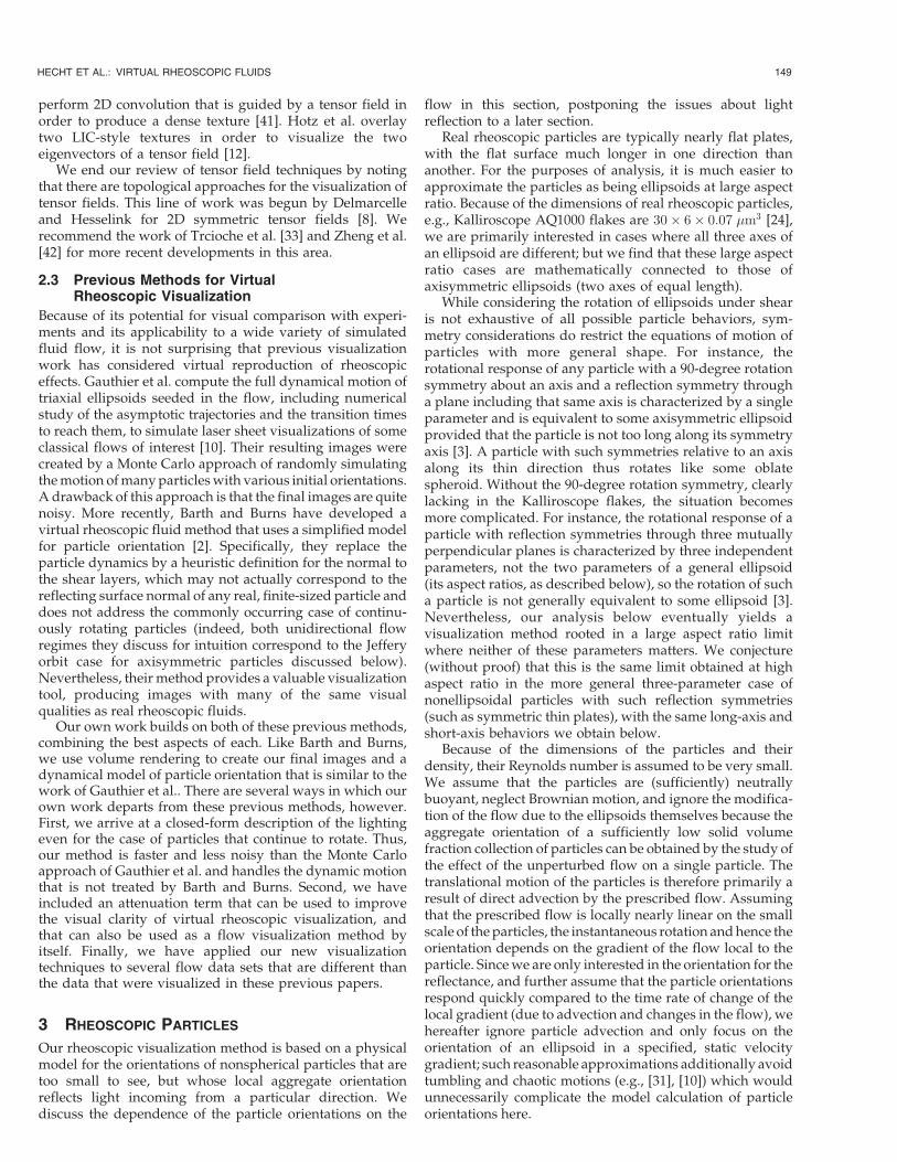
Fig. 7. Simulation of “internal splash.” Note the upward plume of fluid

that is evident in the last two frames.

to 3D data with parabolic dependence visualized using ourfull rheoscopic technique (not shown) yielded images verysimilar to those using only gradient magnitude. In the fully3D simulations of other phenomena considered below, thereflectances based on particle orientations capture morecomplicated details than gradient magnitude alone.

The next CFD simulation that we visualize is the so-called “internal splash” phenomena described by Abaidet al. [1]. When a heavier-than-fluid ball falls through theinterface between light and heavy fluid, the ball maytemporarily bounce upward. We simulated this phenomenausing an Eulerian grid simulation of fluid, using Lagran-gian constraints to cause a portion of the grid to mimic a

solid object [5], [28]. Fig. 7 shows several frames from such asimulation, with virtual rheoscopic particles used to helpvisualize the fluid flow. In the lighter fluid, the particleswere black-and-white, whereas the particles were coloredred in the heavier fluid. In the two upper frames of thefigure, the rheoscopic visualization indicates a region offluid that the ball is pushing in front of itself as it falls. Thecomplexity of the fluid motion when the green ball strikesthe light/heavy fluid interface is evident in the lower twoframes. Also, in these two frames, there is a visualindication of upward motion of fluid above the ball intothe lighter fluid. This motion is even more evident in theaccompanying video, as also are the complicated wavemotions passing though the heavy fluid after the impact.

Fig. 8 shows the 3D nature of the visualization technique.Just one time step is shown in each of these images, but thevoxel grid is rotated to different positions in these images.Fig. 5 shows the effect of moving a virtual light from left toright for a single time step. The virtual rheoscopic particlesreflect light differently depending on the position of thevirtual light source.

The final CFD simulation that we present demonstratesan instability in particle sedimentation (simulated usingdilute-limit interactions as in [27]). Many small, heavyspherical particles are suspended in fluid over a region ofclear (particle-free) liquid at the start of the simulation. Asthe simulation progresses, the spherical particles drop intothe clear liquid. The particles’ motion is not uniform, andcolumns of downward moving particles form that are atleast superficially similar to the fingering that is generatedin a Raleigh-Taylor instability (though in this case, it is amiscible interface). Fig. 9 shows three different visualiza-tions of this simulation data, with fluid velocities evaluatedon a uniform grid (Table 1) from the specified particleforces, with centered-difference evaluation of the velocitygradients on the same grid. The top two images are an earlyand later time step from the simulation showing onlyparticle positions. The motion of the particle-free fluid is notevident from this visualization.

Fig. 9b shows the same two time steps as in the first row,but uses our rheoscopic visualization method in addition toshowing the positions of the falling particles. In thisvisualization, the amount of reflected light in the rheoscopiclighting model is attenuated by the gradient magnitude. Inorder to better show the rheoscopic lighting, only 1/10 ofthe original spherical particles are included in this anima-tion. The positions of the omitted particles are indicated byred coloring of the voxels that contain or are very near thefalling particles. In these middle frames, the rheoscopiclighting of the fluid gives a clear indication of those portionsof the fluid that are in motion. Moreover, the dark and lightchannels that can be seen in the particle-filled regionsindicate that some particle-laden regions are moving fasterthan others. The light regions on top of the particles indicatecolumns of particles that are moving upward. In the


Fig. 8. Internal splash, varying the orientation of the volumetric grid.

TABLE 1Statistics for the Different Sequences Shown in This Paper

particle-only animation of this flow, this variable rate ofparticle motion can only be seen with difficulty. In the stillframes with particles alone, this motion is not evident at all.A close-up of this simulation can also be seen in Fig. 1.

Fig. 9c shows the same simulation data, this timevisualized using rheoscopic lighting alone. None of thefalling particles are shown and the rheoscopic reflectance isnot attenuated by the gradient magnitude. The only indica-tion of the positions of the falling particles is the red color ofthe region near the particles. The most striking thing aboutthese images are the repeated bands of light and dark bothabove and below the particles. It is evident from comparingthis frame to the middle left frame that these bands diminishin strength as one moves further into the particle-free fluiddomain. We were unaware of the presence of these repeatedbands from our earlier particle-based visualizations ofsedimentation. These bands, with separation comparable tothe small out-of-plane dimension of the container (and thus,above the grid scale used for the gradient calculation), appearto correspond to counter-rotating regions which are weaklydecaying in strength moving away from the particles. Suchbehavior is consistent both with the system-size correlationstypical of the velocity fluctuation problem in creeping flowsedimentation and with the well-known presence of suchcounter-rotating flow in the particle-laden region; but onlywhen we viewed this data using the rheoscopic lightingmodel did this aspect of the simulation data become clearaway from the motion of the particles themselves. Also,visible in these two lower images are the slow and fast movingcolumns of particles, coded by dark and light intensities dueto the variation in rheoscopic reflectances.

We have implemented the virtual rheoscopic visualizationmethod of Barth and Burns [2], and include images based ontheir method for comparison to our own rheoscopic lightingmodel. Fig. 10 shows a Barth and Burns style of visualization

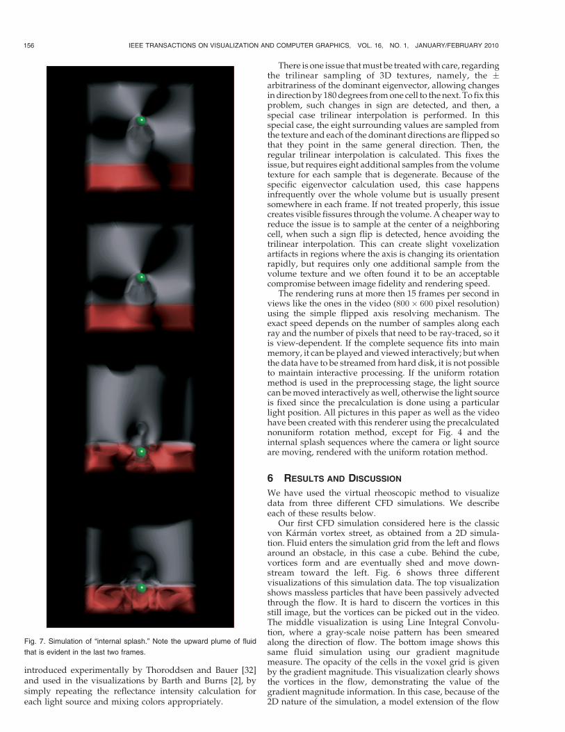
of our particle sedimentation data, which can be compared toour results in Fig. 9. Figs. 11a and 11b show a comparisonbetween our method and Barth and Burns for visualizing theinternal splash data. In each case, the qualitative appearancesof the data sets appear similar, but the actual features that arehighlighted by the two methods differ. In many visualizationsystems, users are given a broad array of visualization stylesto draw upon. Our own rheoscopic lighting model is a newadditional visualization style and it provides an alternative tothe method of Barth and Burns.

Flow visualization for 3D time-varying data is notor-iously difficult. Some of the best methods for visualizingsuch data include placing particles, glyphs, or streamlinesin the flow. Unfortunately, the use of too many suchvisualization primitives can produce cluttered and confus-ing images. Our virtual rheoscopic method offers quite adifferent form of visualization. Our method shows fine flowdetails, and the images that it produces are relativelyuncluttered when compared with most other 3D flowvisualization methods. As with any method, our approachhas some limitations. Perhaps, the biggest limitation of ourvirtual rheoscopic method is that the flow direction at agiven location cannot be determined from a single still


Fig. 9. Particle sedimentation simulation at two time steps. (a) Particles only. (b) Overlays attenuated rheoscopic lighting over the particles.

(c) Unattenuated rheoscopic lighting model. The particle colors used in (a) and (b) are purely for ease of tracking individual particles in the video.

Fig. 10. Barth and Burns style visualization of the sedimentation data.

image. When viewing a sequence of images that werecreated using our method, however, we find that themotion of the fluid is quite easy to see. This can be seenfrom the accompanying video sequences.

7 CONCLUSION

We have presented a method of visualizing 3D time-varying flow fields using a virtual rheoscopic lightingmodel. Inspired by a common fluid dynamics lab tool, ourmethod mimics the reflectance of tiny particles that alignthemselves according to the velocity gradient of a fluid.Using this approach, we produce real-time visualizations oftime-varying 3D flows that are rich in fine details.

There are a number of possible future directions for thiswork. One possibility is to use our virtual rheoscopictechnique together with other flow visualization methods.For example, it may be beneficial to embed oriented glyphs ina virtual rheoscopic simulation. Such a visualization hybridwould show off both fine details (based on the virtualrheoscopic lighting) and also clearly show the direction flowat each glyph. It would also be beneficial to undertake a user’sstudy to see how effective the virtual rheoscopic method is atconveying flow information when compared against otherflow visualization techniques. Our current model treats theparticles as too small to see except in their aggregate lightingeffects. It would be interesting to modify the approach bycreating larger visible particles that are oriented as ours, butthat are also specifically advected through the flow. Finally,many of the most successful computer techniques forperforming flow visualization have been inspired by meth-ods used in real physical experiments. Perhaps, there are stillother flow visualization techniques that are used in experi-mental fluid dynamics labs that can also inspire newcomputer-based visualization methods.

ACKNOWLEDGMENTS

The authors thank Nipun Kwatra, Chris Wojtan, and MarkCarlson for the internal splash simulation code. Thisresearch was funded by US National Science Foundation(NSF) grants CCF-0625190 and CCF-0625264 and by ahardware donation from NVIDIA.

REFERENCES

[1] N. Abaid, D. Adalsteinsson, A. Agyapong, and R.M. McLaughlin,“An Internal Splash: Levitation of Falling Spheres in StratifiedFluids,” Physics of Fluids, vol. 16, no. 5, pp. 1567-1580, May 2004.

[2] W.L. Barth and C.A. Burns, “Virtual Rheoscopic Fluids for FlowVisualization,” IEEE Trans. Visualization and Computer Graphics,vol. 13, no. 6, pp. 1751-1758, Nov./Dec. 2007.

[3] F.P. Bretherton, “The Motion of Rigid Particles in a Shear Flow atLow Reynolds Number,” J. Fluid Mechanics, vol. 14, pp. 284-304,1962.

[4] B. Cabral and L. Leedom, “Imaging Vector Fields Using LineIntegral Convolution,” Proc. ACM SIGGRAPH ’93, pp. 263-270,Aug. 1993.

[5] M. Carlson, P.J. Mucha, and G. Turk, “Rigid Fluid: Animating theInterplay between Rigid Bodies and Fluid,” Proc. ACM SIG-GRAPH ’04, pp. 377-384, Aug. 2004.

[6] R. Crawfis and N. Max, “Direct Volume Visualization of ThreeDimensional Vector Fields,” Proc. Workshop Volume Visualization,pp. 55-60, 1992.

[7] T. Delmarcelle and L. Hesselink, “Visualization of Second OrderTensor Fields and Matrix Data,” Proc. IEEE Conf. Visualization,pp. 316-323, Oct. 1992.

[8] T. Delmarcelle and L. Hesselink, “The Topology of Symmetric,Second-Order Tensor Fields,” Proc. IEEE Conf. Visualization,pp. 140-147, Oct. 1994.

[9] D. Dovey, “Vector Plots for Irregular Grids,” Proc. IEEE Conf.Visualization, pp. 248-253, Oct./Nov. 1995.

[10] G. Gauthier, P. Gondret, and M. Rabaud, “Motions of AnisotropicParticles: Application to Visualization of Three-DimensionalFlows,” Physics of Fluids, vol. 10, pp. 2147-2154, Sept. 1998.

[11] I. Grant, “Particle Image Velocimetry: A Review,” Proc. Inst. ofMechanical Engineers, Part C, vol. 211, no. 1, pp. 55-76, 1997.

[12] I. Hotz, L. Feng, H. Hagen, B. Hamann, K. Joy, and B. Jeremic,“Physically Based Methods for Tensor Field Visualization,” Proc.IEEE Conf. Visualization, pp. 123-130, Oct. 2004.

[13] T.J. Jankun-Kelly and K. Mehta, “Superellipsoid-Based RealSymmetric Traceless Tensor Glyphs Motivated by Nematic LiquidCrystal Alignment Visualization,” Proc. IEEE Conf. Visualization,pp. 1197-1204, Oct./Nov. 2006.

[14] G.B. Jeffery, “The Motion of Ellipsoidal Particles Immersed in aViscous Fluid,” Proc. Royal Soc. of London, Series A, vol. 102,pp. 161-179, 1922.

[15] B. Jobard and W. Lefer, “Creating Evenly-Spaced Streamlines ofArbitrary Density,” Proc. Eurographics Workshop Visualization inScientific Computing, pp. 43-55, Oct. 1998.

[16] J.T. Kajiya and T.L. Kay, “Rendering Fur with Three DimensionalTextures,” Proc. ACM SIGGRAPH ’89, pp. 271-280, July/Aug.1989.

[17] G. Kindlmann and D. Weinstein, “Hue-Balls and Lit-Tensors forDirect Volume Rendering of Diffusion Tensor Fields,” Proc. IEEEConf. Visualization, pp. 183-189, Oct. 1999.


Fig. 11. Internal splash comparison between (a) our rheoscopic lighting model and (b) that of Barth and Burns.

[18] G. Kindlmann, D. Weinstein, and D. Hart, “Strategies for DirectVolume Rendering of Diffusion Tensor Fields,” IEEE Trans.Visualization and Computer Graphics, vol. 6, no. 2, pp. 124-138,Apr.-June 2000.

[19] G. Kindlmann, D. Weinstein, and D. Hart, “Strategies for DirectVolume Rendering of Diffusion Tensor Fields,” Proc. IEEE Conf.Visualization, pp. 1329-1335, Oct./Nov. 2006.

[20] D.H. Laidlaw, E.T. Ahrens, D. Kremers, M.J. Avalos, R.E. Jacobs,and C. Readhead, “Visualizing Diffusion Tensor Images of theMouse Spinal Cord,” Proc. IEEE Conf. Visualization, pp. 127-134,Oct. 1998.

[21] R.S. Laramee, B. Jobard, and H. Hauser, “Image Space BasedVisualization of Unsteady Flow on Surfaces,” Proc. IEEE Conf.Visualization, pp. 131-138, Oct. 2003.

[22] R.S. Laramee, H. Hauser, H. Doleisch, B. Vrolijk, F.H. Post, and D.Weiskopf, “The State of the Art in Flow Visualization: Dense andTexture-Based Techniques,” Computer Graphics Forum, vol. 23,no. 2, pp. 203-221, 2004.

[23] Z. Liu, R.J. Moorhead, and J. Groner, “An Advanced Evenly-Spaced Streamline Placement Algorithm,” Proc. IEEE Conf.Visualization, pp. 965-972, Oct./Nov. 2006.

[24] P. Matisse and M. Gorman, “Neutrally Buoyant AnisotropicParticles for Flow Visualization,” Physics of Fluids, vol. 27, no. 4,pp. 759-760, Apr. 1984.

[25] O. Mattausch, T. Theußl, H. Hauser, and E. Groller, “Strategies forInteractive Exploration of 3D Flow Using Evenly-Spaced Illumi-nated Streamlines,” Proc. Spring Conf. Computer Graphics, pp. 213-222, Apr. 2003.

[26] A. Mebarki, P. Alliez, and O. Devillers, “Farthest Point Seeding forEfficient Placement of Streamlines,” Proc. IEEE Conf. Visualization,pp. 479-486, Oct. 2005.

[27] P.J. Mucha, S.-Y. Tee, D.A. Weitz, B.I. Shraiman, and M.P.Brenner, “A Model for Velocity Fluctuations in Sedimentation,”J. Fluid Mechanics, vol. 501, pp. 71-104, 2004.

[28] N.A. Patankar, P. Singh, D.D. Joseph, R. Glowinski, and T.-W.Pan, “A New Formulation of the Distributed Lagrange Multi-plier/Fictitious Domain Method for Particulate Flows,” Int’l J.Multiphase Flow, vol. 26, no. 9, pp. 1509-1524, 2000.

[29] T. Preußer and M. Rumpf, “Anisotropic Nonlinear Diffusion inFlow Visualization,” Proc. IEEE Conf. Visualization, pp. 325-332,Oct. 1999.

[30] A.R. Sanderson, C.R. Johnson, and R.M. Kirby, “Display of VectorFields Using a Reaction-Diffusion Model, Visualization Techni-ques,” Proc. IEEE Conf. Visualization, pp. 115-122, Oct. 2004.

[31] S. Omer, “On Flow Visualization Using Reflective Flakes,” J. FluidMechanics, vol. 152, pp. 235-248, 1985.

[32] S.T. Thoroddsen and J.M. Bauer, “Qualitative Flow VisualizationUsing Colored Lights and Reflective Flakes,” Physics of Fluids,vol. 11, pp. 1702-1705, 1999.

[33] X. Tricoche, G. Scheuermann, and H. Hagen, “Tensor TopologyTracking: A Visualization Method for Time-Dependent 2DSymmetric Tensor Fields,” Computer Graphics Forum, vol. 20,no. 3, pp. 461-470, 2001.

[34] G. Turk and D. Banks, “Image-Guided Streamline Placement,”Proc. ACM SIGGRAPH ’96, pp. 453-460, Aug. 1996.

[35] J.J. van Wijk, “Spot Noise: Texture Synthesis for Data Visualiza-tion,” Proc. ACM SIGGRAPH ’91, pp. 309-318, July 1991.

[36] J.J. van Wijk, “Image Based Flow Visualization,” Proc. ACMSIGGRAPH ’02, pp. 745-754, July 2002.

[37] J.J. van Wijk, “Image Based Flow Visualization for CurvedSurface,” Proc. IEEE Conf. Visualization ’03, pp. 123-130, Oct. 2003.

[38] V. Verma, D.L. Kao, and Alex Pang, “A Flow-Guided StreamlineSeeding Strategy,” Proc. IEEE Conf. Visualization, pp. 415-422, Oct.2000.

[39] D. Weinstein, G. Kindlmann, and E. Lundberg, “Tensorlines:Advection-Diffusion Based Propagation through Diffusion TensorFields,” Proc. IEEE Conf. Visualization, pp. 249-253, Oct. 1999.

[40] X. Ye, D.L. Kao, and A. Pang, “Strategy for Seeding 3DStreamlines,” Proc. IEEE Conf. Visualization, pp. 471-478, Oct. 2005.

[41] X. Zheng and A. Pang, “HyperLIC,” Proc. IEEE Conf. Visualization2003, pp. 249-256, Oct. 2003.

[42] X. Zheng, B. Parlett, and A. Pang, “Topological Structures of 3DTensor Fields,” Proc. IEEE Conf. Visualization, pp. 551-558, Oct.2005.

[43] L. Zhukov and A. Barr, “Oriented Tensor Reconstruction: TracingNeural Pathways from Diffusion Tensor MRI,” Proc. IEEE Conf.Visualization, pp. 387-394, Oct./Nov. 2002.

Florian Hecht received the Diplom in computerscience from the University of Karlsruhe, Ger-many, in 2008, and the MS degree in computerscience from the Georgia Institute of Technologyin 2007. He began work on his PhD degree in Fall2009 at the University of California, Berkeley. Heis interested in computer graphics, robotics, andcomputer vision.

Peter J. Mucha received the PhD degree inapplied and computational mathematics fromPrinceton University in 1998. He was an appliedmathematics instructor at the MassachussettsInstitute of Technology (MIT) for three years,followed by four years as an assistant professor inmathematics at Georgia Institute of Technology.He is currently an associate professor at theUniversity of North Carolina at Chapel Hill, wherehe is a member of the Department of Mathematics

and the Institute for Advanced Materials, Nanoscience & Technology.

Greg Turk received the PhD degree in compu-ter science from the University of North Carolinaat Chapel Hill (UNC) in 1992. He was apostdoctoral researcher at Stanford Universityfor two years, followed by two years as aresearch scientist at UNC Chapel Hill. He iscurrently a professor at the Georgia Institute ofTechnology, where he is a member of theSchool of Interactive Computing and the Gra-phics, Visualization and Usability Center. His

research interests include computer graphics, scientific visualization,and computer vision. In 2008, he was the technical papers chair forACM SIGGRAPH. He is a member of the IEEE.

. For more information on this or any other computing topic,please visit our Digital Library at www.computer.org/publications/dlib.


ieee transactions on visualization and ...turk/my_papers/rheoscopic_fluids.pdf3d velocity fields. by...

Documents