ieice communications express, vol.6, no.2, 65 low ... letter assumes a dl-mu-mimo-ofdm system in...

Low complexity non-linearpre-coding on downlinkmultiuser MIMO systems

Tomoki Murakamia), Koichi Ishihara, Hirantha Abeysekera,Yasushi Takatori, and Masato MizoguchiNTT Access Network Service Systems Laboratories, Nippon Telegraph and

Telephone Corporation, 1–1 Hikarinooka, Yokosuka, Kanagawa 239–0847, Japan

a) [email protected]

Abstract: This paper proposes low complexity non-linear pre-coding that

switching among pre-coding weights per orthogonal frequency division

multiplexing (OFDM) symbol according to the modulation scheme and

constellation point of users, for downlink multiuser multiple input multiple

output (DL-MU-MIMO) systems. In the proposed pre-coding, when some

users have the same modulation scheme and constellation point, the pre-

coding weight is calculated based on broadcast approach without inter-user

interference cancellation. If not, the pre-coding weight is calculated based on

unicast approach such as the zero-forcing (ZF) method. In addition, com-

puter simulation results show that the proposed pre-coding achieves lower bit

error rate (BER) on low signal to noise ratio (SNR) environments.

Keywords: downlink multiuser multiple input multiple output (DL-MU-

MIMO), non-linear pre-coding, wireless LAN system

Classification: Wireless Communication Technologies

References

[1] Wireless LAN Medium Access Control (MAC) and Physical Layer (PHY)Specifications, IEEE Std. 802.11ac-2013.

[2] 3GPP TS 36.913, “Evolved Universal Terrestrial Radio Access (E-UTRA);Requirements for further advancements for Evolved Universal Terrestrial RadioAccess (EUTRA) LTE-Advanced”.

[3] H. Spencer, C. B. Peel, A. L. Swindlehurst, and M. Haardt, “An introductionto the multi-user MIMO downlink,” IEEE Commun. Mag., vol. 42, no. 10,pp. 60–67, Oct. 2004. DOI:10.1109/MCOM.2004.1341262

[4] R. Fischer, C. Windpassinger, A. Lampe, and J. Huber, “Space time transmissionusing Tomlinson-Harashima precoding,” Proc. 4th ITG Conf. Source ChannelCoding, Berlin, Germany, Jan. 2002, pp. 139–147.

[5] C. Peel, B. Hochwald, and L. Swindlehurst, “Avector-perturbation technique fornear-capacity multi-antenna multi-user communication,” Proc. 41st AllertonConf. Communication, Control, Computing, IL, Oct. 1–3, 2003.

© IEICE 2017DOI: 10.1587/comex.2016XBL0177Received October 3, 2016Accepted October 24, 2016Publicized November 15, 2016Copyedited February 1, 2017

65

IEICE Communications Express, Vol.6, No.2, 65–70

http://dx.doi.org/10.1109/MCOM.2004.1341262




1 Introduction

In order to achieve high-speed and high-efficiency wireless transmission, downlink

multiuser multiple input multiple output (DL-MU-MIMO) transmission is adopted

in IEEE 802.11ac [1] and 3GPP long term evolution (LTE) advanced [2]. In DL-

MU-MIMO systems, base station (BS) simultaneously transmits to multiple users

on the same frequency channel while using pre-coding techniques to mitigate inter-

user interference [3]. Especially, it is expected that DL-MU-MIMO transmission

can improve total throughput in practical environments where most users will

utilize just a few antennas for compactness and low cost.

Maximizing the channel capacity of DL-MU-MIMO transmission demands

propagation environments with high signal to noise ratios (SNRs) between BS and

user antennas and low spatial correlation between user antennas. Therefore, it is

important to improve DL-MU-MIMO transmission in practical environments

including those with low SNR values and high spatial correlation. In order to

realize these improvements, non-linear pre-coding techniques such as Tomlinson-

Harashima precoding (THP), vector perturbation (VP), have been investigated in

[4, 5]. However, it is known that accurate channel state information (CSI) and large

computing resources are required which complicates practical realization.

In this letter, we propose low complexity non-linear pre-coding for DL-MU-

MIMO systems in low SNR conditions. In the proposed pre-coding, several pre-

coding weights, generated to suit modulation schemes and constellation points of

users, are activated for different orthogonal frequency division multiplexing

(OFDM) symbol. By applied a limited number of pre-coding weights to each

OFDM symbol, computational complexity is suppressed from that incurred by non-

linear pre-coding techniques. Our computer simulation results clarify the effective-

ness of DL-MU-MIMO with the proposed pre-coding by comparing it to conven-

tional pre-coding on low SNR conditions.

2 System model

This letter assumes a DL-MU-MIMO-OFDM system in which transmitter (TX)

transmits to N receivers (RXs). TX has M antennas while each RX has single

antenna. hnðkÞ denotes CSI of the kth (k ¼ 1 . . .K) subcarrier between TX and RX-n

(n ¼ 1 . . .N). The received signals at RX-n, ynðkÞ, are expressed by the transmit

signal, x1ðkÞ � xNðkÞ, as

ynðkÞ ¼ hnðkÞwnðkÞxnðkÞ þXN

l¼1;l≠nhlðkÞwlðkÞxlðkÞ þ nnðkÞ; ð1Þ

where wnðkÞ is the pre-coding weight of DL-MU-MIMO for RX-n, and nnðkÞ is anadditive white Gaussian noise vector with variance of �2. For DL-MU-MIMO

transmission, we assume that equal power is allocated to each RX because each RX

will demand the same communication quality. In addition, for practical use, the pre-

coding weight equivalent to the conventional pre-coding case, wnCðkÞ, is calculated

by channel inversion based on zero-forcing (ZF) [3], which is a low complexity

weight calculation method expressed by© IEICE 2017DOI: 10.1587/comex.2016XBL0177Received October 3, 2016Accepted October 24, 2016Publicized November 15, 2016Copyedited February 1, 2017

66


wCn ðkÞ ¼

w0Cn ðkÞ

kw0Cn ðkÞkF

; ð2Þ

w0C1 ðkÞ � � � w0C

n ðkÞ � � � w0CN ðkÞ� � ¼ HCðkÞHðHCðkÞHCðkÞHÞ�1; ð3Þ

where kAkF is the Frobenius norm of A, and HCðkÞ is expressed as

HCðkÞ ¼ h1ðkÞT � � � hnðkÞT � � � hNðkÞT� �T

; ð4Þwhere AT is the transpose operator of A.

3 Low complexity non-linear pre-coding

This section explains the proposed low complexity non-linear pre-coding for DL-

MU-MIMO transmission. Its chief characteristic is to assume that the modulation

schemes and constellation points of users in low SNR environments are likely to be

the same. In the proposed pre-coding, several pre-coding weights, derived accord-

ing to modulation schemes and constellation points of users, are switched for each

OFDM symbol. Fig. 1 shows an example of the proposed pre-coding using BPSK

and two users. As shown in Fig. 1(b), when a user set with the same modulation

scheme and constellation point exists, the pre-coding weight is calculated based on

broadcast without inter-user interference cancellation. In order to improve channel

capacity, the pre-coding weight on broadcast, wbBðkÞ, defines as

wBb ðkÞ ¼ VðNÞðkÞ�v1ðkÞ; ð5Þ

where b (b ¼ 1; . . . ; B) denotes the user index with the same modulation scheme

and constellation point and VðNÞðkÞ is the matrix combined from right singular

vectors on null space of matrix HBðkÞ including CSI of users with different

modulation schemes and constellation points as calculated by

HBðkÞ ¼ h1ðkÞT � � � huðkÞT � � � hUðkÞT� �T ¼ UðkÞ�ðkÞ VðSÞðkÞ VðNÞðkÞ

� �H;

ð6Þwhere AH denotes the Hermitian transpose operator of A, u (u ¼ 1; . . . ; U) is the

user index for the difference modulation scheme and constellation points, UðkÞ isthe matrix combined from the left singular vectors, �ðkÞ is the diagonal matrix in

which the diagonal elements represent the square roots of the eigenvalues, and

VðSÞðkÞ is the matrix combined from right singular vectors on signal space. �v1ðkÞ isthe right singular vector of maximum eigenvalue as calculated by

�HBðkÞVðNÞðkÞ ¼ h1ðkÞT � � � hbðkÞT � � � hBðkÞT� �T

VðNÞðkÞ¼ �UðkÞ ��ðkÞ �v1ðkÞ � � � �vbðkÞ � � � �vBðkÞ

� �H ; ð7Þ

where �HBðkÞ is the matrix including CSI of users with the same modulation scheme

and constellation points.

On the other hand, another pre-coding weight, wuUðkÞ, is calculated based on

unicast with inter-user interference cancellation such as the ZF method [3]. In this

letter, the pre-coding weight on unicast is calculated by Eq. (8)–(10).

wUu ðkÞ ¼

w0Uu ðkÞ

kw0Uu ðkÞkF

; ð8Þ© IEICE 2017DOI: 10.1587/comex.2016XBL0177Received October 3, 2016Accepted October 24, 2016Publicized November 15, 2016Copyedited February 1, 2017

67


w0U1 ðkÞ � � � w0U

U ðkÞ w0UUþ1ðkÞ � � � w0U

UþbðkÞ � � � w0UUþBðkÞ

� �¼ HUðkÞHðHUðkÞHUðkÞHÞ�1

; ð9Þ

HUðkÞ ¼�HBðkÞHBðkÞ

" #; ð10Þ

4 Simulation results

This section evaluates the effectiveness of the proposed pre-coding through com-

puter simulation based on the IEEE 802.11ac standard [1]. Table I shows the

simulation parameters. Frequency and bandwidth are 5GHz and 80MHz, respec-

tively. The numbers of TX and RX antennas are from two to four and one,

respectively. The number of RXs runs from two to four matching the number of

TX antennas. Assuming low SNR environments, the modulation scheme is set to

BPSK or QPSK. In addition, we assume that the propagation channel is channel

model B [1] and that SNR ranges from 0 to 20 dB.

Fig. 2 shows the simulation results of DL-MU-MIMO transmission with and

without the proposed pre-coding. First, Fig. 2(a) shows the average bit error rate

Table I. Computer simulation parameters

Frequency 5GHz

Bandwidth 80MHz

Number of TX antennas 2, 3, 4

Number of RX antennas 1

Number of RXs 2, 3, 4

Modulation scheme BPSK, QPSK

(a) Conventional pre-coding.

(b) Proposed pre-coding.

Fig. 1. Concept of the proposed pre-coding.


68


(BER) performance of the proposed and conventional pre-coding approaches when

SNR varies from 0 to 20 dB. In this simulation, we assume that a TX with two

antennas uses DL-MU-MIMO transmission to transmit to two RXs. Thus BER is

averaged over all RXs. As shown in Fig. 2(a), it can been seen that the proposed

pre-coding by using just two weights offers improvements of 2.5 dB under BPSK

and 1.2 dB under QPSK from the conventional pre-coding at BER ¼ 10�2. This isbecause the received power per RX is increased by using broadcast pre-coding

weight without interference cancellation. Moreover, BPSK offers greater improve-

(a) Average BER versus SNR.

(b) Number of RX versus BER=10-2 improvement performance.

Fig. 2. Computer simulation results


69


ment QPSK. This is that, BPSK doubles the probability the shared use of

modulation scheme and constellation points compared to QPSK.

Second, we elucidate the impact of the number of RXs. Fig. 2(b) shows the

performance improvements possible with BPSK and QPSK at BER ¼ 10�2 when

the number of RXs ranges from two to four. The number of TX antennas equals the

number of RXs. From the results of Fig. 2(b), we found that BER performance

improvements strengthen with the number of RXs. This is because the probability

of modulation scheme and constellation point sharing is raised by increasing the

number of RXs. Moreover, BPSK offers greater improvement than QPSK as

observed in Fig. 2(a).

5 Conclusion

In this letter, we proposed low complexity non-linear pre-coding for DL-MU-

MIMO systems. The proposed pre-coding switching among several pre-coding

weights for each OFDM symbol according to modulation schemes and constella-

tion points of users. If a set of users adopt the same modulation schemes and

constellation points, the pre-coding weight is calculated based on broadcast

approach without inter-user interference cancellation. On the other hand, if the

set adopt difference modulation schemes and constellation points, the pre-coding

weight is calculated based on the unicast approach with inter-user interference

cancellation. Computer simulations confirmed that the proposed pre-coding offers

improvements of 2.5 dB under BPSK and 1.2 dB under QPSK from conventional

pre-coding at BER ¼ 10�2. Moreover, we clarify that the proposed pre-coding can

achieve further improvements as the number of users is increased.


70


Experimental evaluation ofinterference reduction effect;Eigen-beamforming anddigital subtraction by usingMIMO-OFDM signals

Yoshiyuki Yamamoto1, Ryota Takahashi2†, Masakuni Tsunezawa2,Naoki Honma2a), and Kentaro Murata31 Faculty of Engineering, Iwate University,

4–3–5 Ueda, Morioka 020–8551, Japan2 Graduate School of Engineering, Iwate University,

4–3–5 Ueda, Morioka 020–8551, Japan3 Graduate School of Engineering, National Defense Academy,

1–10–20 Hashirimizu, Yokosuka, Kanagawa 239–8686, Japan


Abstract: In this letter, we experimentally validate an interference reduc-

tion technique that combines a digital subtraction technique, and eigen-

beam-forming with an end-fire arrangement of linear array antennas. The

eigen-beamforming significantly reduces the self-interference at the cost of

a slight drop in the degrees-of-freedom of the antenna. We experimentally

evaluate the degree of interference reduction using two linear sleeve-dipole

arrays in end-fire arrangement. This experiment uses MIMO (Multiple-Input

Multiple-Output)-OFDM (Orthogonal Frequency Division Multiplexing)

signals to evaluate the realistic performance of this technique. The results

of the experiment show the combination of eigen-beamforming and digital

subtraction can significantly reduce, −76 dB, the interference.

Keywords: full-duplex, interference, beamforming, digital subtraction

Classification: Antennas and Propagation

References

[1] S. Hong, J. Brand, J. Choi, M. Jain, J. Mehlman, S. Katti, and P. Levis,“Applications of self-interference cancellation in 5G and beyond,” IEEECommun. Mag., vol. 52, no. 2, pp. 114–121, Feb. 2014. DOI:10.1109/MCOM.2014.6736751

[2] D. Senaratne and C. Tellambura, “Beamforming for space division duplexing,”Proc. IEEE Int. Conf. Commun., pp. 1–5, Jun. 2011. DOI:10.1109/icc.2011.5962761

[3] N. Li, W. Zhu, and H. Han, “Digital interference cancellation in single channel,full duplex wireless communication,” 2012 8th Int. Conf. Wireless Commun.,

†Ryota Takahashi sadly passed away on 17th Nov. 2016

© IEICE 2017DOI: 10.1587/comex.2016XBL0175Received September 29, 2016Accepted October 25, 2016Publicized November 22, 2016Copyedited February 1, 2017

71






http://dx.doi.org/10.1109/icc.2011.5962761




Networking and Mobile Comput. (WiCOM), pp. 1–4, Sept. 2012. DOI:10.1109/WiCOM.2012.6478497

[4] T. Riihonen and R. Wichman, “Analog and digital self-interference cancellationin full-duplex MIMO-OFDM transceivers with limited resolution in A/Dconversion,” Proc. 46th Asilomar Conf. Signals, Syst. and Comput., pp. 45–49,Nov. 2012. DOI:10.1109/ACSSC.2012.6488955

[5] J. I. Choi, M. Jain, K. Srinivasan, P. Levis, and S. Katti, “Achieving singlechannel, full duplex wireless communication,” Proc. 2010 ACM MobiCom.,pp. 1–12, Sept. 2010. DOI:10.1145/1859995.1859997

[6] M. Jain, J. I. Choi, T. Kim, D. Bharadia, S. Seth, K. Srinivasan, P. Levis, S.Katti, and P. Sinha, “Practical, real-time, full duplex wireless,” Proc. 2011 ACMMobiCom., pp. 301–312, Sept. 2011. DOI:10.1145/2030613.2030647

[7] M. Tsunezawa, N. Honma, K. Takahashi, Y. Tsunekawa, K. Murata, and K.Nishimori, “Interference reduction between SDD linear array antennas usingend-fire arrangement,” 2015 IEEE International Symposium on Antennas andPropagation & USNC/URSI National Radio Science Meeting, pp. 2511–2512,Jul. 2015. DOI:10.1109/APS.2015.7305644

1 Introduction

Full-duplex communication is being studied recently for application to the 5G

wireless network [1]. Full-duplex communication establishes two-way communi-

cation using the same frequency and time resources [2]. However, full-duplex

communication cannot be realized without resolving the self-interference problem,

i.e. the strong transmitting signal is captured by its receiving antennas which

interferes with the desired receiving signals. Ideally, self-interference can be

eliminated by digital subtraction since the self-interference is known signal [3].

However, the self-interference is significantly stronger than the desired signal, and

causes RF (Radio Frequency) front-end saturation, which produces nonlinear signal

distortion. In this case, digital subtraction is unable to adequately suppress the

self-interference [4]. Therefore, the self-interference needs to be suppressed before

the RF front-end at the receiver. To combat this, three methods have been studied

[5, 6, 7]. Antenna cancellation uses an additional transmitting antenna to form a null

point at the receiving antenna [5]. Balun cancellation places a balun circuit between

the transmitting and receiving antennas to subtract the self-interference signals from

the received signals [6]. Note that these methods cannot be directly applied to

MIMO systems because the interference among all combinations of transmitting and

receiving antennas must be considered and implementation is difficult. To resolve

this problem, eigen-beamforming using linear array antennas in the end-fire arrange-

ment was proposed for self-interference reduction in the MIMO full-duplex system

[7]. This method offers very high interference reduction with the consumption of

only one degree-of-freedom of the antenna array; this antenna arrangement degen-

erates the rank of the interference channel to 1. Only the S-parameter of the antennas

has been used to verify the performance of this method, meaning that the total

cancellation performance, including signal subtraction, has yet to be evaluated.

This letter experimentally evaluates the interference cancellation performance

of the method proposed in [7] by using real MIMO-OFDM signals. A signal frame-


72


http://dx.doi.org/10.1109/WiCOM.2012.6478497





http://dx.doi.org/10.1109/ACSSC.2012.6488955




http://dx.doi.org/10.1145/1859995.1859997

http://dx.doi.org/10.1145/1859995.1859997

http://dx.doi.org/10.1145/1859995.1859997

http://dx.doi.org/10.1145/2030613.2030647

http://dx.doi.org/10.1145/2030613.2030647

http://dx.doi.org/10.1145/2030613.2030647

http://dx.doi.org/10.1109/APS.2015.7305644




format is newly developed for this experiment, and the total performance of the

self-interference reduction method including digital subtraction technique is inves-

tigated, where the remaining interference caused by the saturation of the RF front-

end and imperfection of the antenna arrangement is evaluated.

2 Self-interference reduction method using eigen-beamforming and

digital subtraction

Fig. 1(a) shows a system model of the in-house-developed full-duplex testbed with

linear array antennas in the end-fire arrangement. M and N are the number of

transmitters (Tx) and receivers (Rx), respectively, H is the interference channel,

and s is the transmission signal. Let us describe the eigen-beamforming scheme in

this experiment. The singular value decomposition of the interference channel H is

given by

H ¼ U�VH; ð1Þwhere f�gH represents Hermitian transpose. V and U are eigen-vector matrices of

Tx and Rx, respectively. The number of eigen-values is given by

Fig. 1. System model and MIMO-OFDM frame format


73


Ni ¼ minðM;NÞ; ð2Þand V and � are defined by

V ¼ ½v1; v2; � � � ; vM� ð3Þ� ¼ diagð ffiffiffiffiffi

�1p

;ffiffiffiffiffi�2

p; � � � ; ffiffiffiffiffiffi

�Ni

p Þ; ð4Þwhere vi is the i-th transmission weight vector, and �i is the i-th eigen-value. The

eigen-values correspond to the received signal strength of the eigen-modes. Eigen-

beamforming is the interference reduction technique that uses the eigen-mode

weight vector described in (3). The i-th transmission mode is formed by the i-th

transmission weight vector. In the eigen-beamforming scheme, the eigen-vectors

excluding those corresponding to several of the largest eigen-values are used. This

lowers the degree-of-freedoms of the antennas, where the number is determined

by the number of suppressed modes. When transmitting and receiving linear array

antennas are placed in an end-fire arrangement, the rank of the transmission modes

is expected to degenerate to 1. This means, the required number of the antenna-

degrees-of-freedom is minimized to 1, ideally. However, the rank of the interfer-

ence channel in the actual antenna array cannot made 1 because of the channel

imperfections created by the mutual coupling among the antennas and the finite

distance between the transmitting and receiving arrays. The self-interference

remains as the interference channel is imperfect. The remaining interference can

be digitally subtracted because the transmitted signals are known. If transmit-

beamforming is not used, the interference signals significantly impact the RF front-

end at its receiver, and subtraction become ineffective as the interfering signals are

nonlinearly distorted.

Fig. 1(b) shows the frame format of the MIMO-OFDM signals. SP (Short

Pramble) synchronizes Tx and Rx, and LP (Long Preamble) is used to estimate the

interference channel. LPi;j and DATAi;j are the signals for j-th eigen-modes

transmitted from the i-th antenna. The interference power is defined by the DATA

signals observed at the receiver. In this scheme, the first channel estimation

(w/oBF LP) is performed to get the interference channel H. Eigen-beamforming

is realized by using the transmission weight matrix consisting of eigen-vectors,

½v2; � � � ; vM�. The second channel estimation (w/BF LP) is also performed to

estimate the interference channel, where the transmission weight without the major

interference mode is used at Tx side. The received signal after digital subtraction is

given by

ySUB ¼ y �Hi~V1s; ð5Þ

where ySUB is the received signal after digital subtraction, y is the received signal,

and s is the transmitted signal.

3 Experiments using MIMO-OFDM signals

3.1 Experimental setup

Fig. 2 shows the measurement environment. The transmitting and receiving anten-

nas are linear array antennas consisting of four element half-wavelength sleeve

antennas. The center frequency is 2.47GHz. For the linear array antennas, the


74


center-to-center distance between Tx and Rx is dTx-Rx ¼ 10�0 (�0: wavelength in a

vacuum), and the element spacing delement is changed from 0:25�0 to 1:5�0. Sheet-

like microwave absorbers are placed below the antennas in order to prevent

reflection from the fixtures.

3.2 Simulation results

Fig. 3(a) shows the eigen-value distribution versus element spacing. The maximum

difference between the first and second eigen-values is 32 dB at delement ¼ 0:25�0,

and the minimum difference is 23 dB at delement ¼ 1:5�0. From this result, the eigen-

Tx Rx

dTx-Rx

dElementSleeve antennas

Microwave absorbers

Fig. 2. Measurement environment

Fig. 3. Measured results


75


weight without first eigen-mode can suppress the interference by more than 23 dB.

Further, the narrower the element spacing becomes, the more eigen-beamforming

suppresses the interference.

Fig. 3(b) shows the interference level versus element spacing. The interference

level is defined as the level of the total received power at Rx side relative to the

total input power at Tx side. Comparing the interference levels without eigen-

beamforming (w/o BF) and with eigen-beamforming (w/ BF) shows that eigen-

beamforming suppresses the interference by at least 20 dB for all element spacing’s

examined. We also found the minimum interference level, −64 dB, is achieved witheigen-beamforming at delement ¼ 0:5�0. The combination of an eigen-beamforming

and digital subtraction (w/ BF + Sub) can suppress the interference to −76 dB at

delement ¼ 0:5�0, which is 12 dB lower than that without subtraction. This result

shows that digital subtraction further suppresses the self-interference power.

4 Conclusion

Experiments confirmed that our combination of eigen-beamforming and digital

subtraction, where linear array antennas in end-fire arrangement are used, can

significantly reduce the self-interference reduction. When the element spacing is

delement ¼ 0:5�0, the interference level reduction achieved by eigen-beamforming

is −64 dB, while with eigen-beamforming and digital subtraction the reduction is

−76 dB. Further interference reduction is needed to implement this technique in

actual full-duplex systems and will be the target of future work.

Acknowledgments

This research and development work was supported by the MIC/SCOPE

#155002002.


76


Demonstration of wirelesstwo-way interferometry(Wi-Wi)

Nobuyasu Shiga1,2a), Kohta Kido1, Satoshi Yasuda1, Bhola Panta1,Yuko Hanado1, Seiji Kawamura1, Hiroshi Hanado1,Kenichi Takizawa1, and Masugi Inoue11 National Institute of Information and Communications Technology (NICT),

4–2–1 Nukui-Kitamachi, Koganei, Tokyo 184–8795, Japan2 PRESTO, Japan Science and Technology (JST),

4–1–8 Honcho Kawaguchi, Saitama 332–0012, Japan


Abstract: Wireless two-way interferometry (Wi-Wi) is the simplified ver-

sion of “carrier phase based two-way satellite time and frequency transfer,”

wherein a wireless communication technology is used instead of a satellite

communication technology. We used the carrier phase of a 2.4GHz ZigBee

module to measure the variation of two rubidium clocks at remote sites.

Since clocks in the ZigBee module are much less precise than rubidium

clocks, the carrier phase of the ZigBee signal cannot be used to compare

two rubidium clocks in a simple manner. Using a technique to cancel the

clock error of transmitters, we demonstrated picosecond-level precision

measurement of the time variation of clocks between two remote systems.

This synchronization technique at picosecond-level precision opens the door

to low-cost wireless positioning at millimeter accuracy.

Keywords: time synchronization, precision motion sensing, ranging

Classification: Wireless Communication Technologies

References

[1] D. W. Hanson, “Fundamentals of two-way time transfers by satellite,” Proc. ofthe 43rd Annual Symposium on Frequency Control, 1989.

[2] M. Fujieda, T. Gotoh, F. Nakagawa, R. Tabuchi, M. Aida, and J. Amagai,“Carrier-phase-based two-way satellite time and frequency transfer,” IEEETrans. Ultrason. Ferroelectr. Freq. Control, vol. 59, pp. 2625–2630, 2012.DOI:10.1109/TUFFC.2012.2503

1 Introduction

Time synchronization plays an important role in our lives. Many areas of informa-

tion and communication technologies, for example, modern computer networks and

wired and wireless communication networks require precise time synchronization.

Similarly, infrastructures such as smart grids and positioning systems require time

© IEICE 2017DOI: 10.1587/comex.2016XBL0181Received October 12, 2016Accepted November 1, 2016Publicized November 25, 2016Copyedited February 1, 2017

77


http://dx.doi.org/10.1109/TUFFC.2012.2503




synchronization, which shows how critical it is to have a properly synchronized

system.

Today, increasingly more devices are being equipped with wireless communi-

cation capabilities, and our goal is to demonstrate that commercial communication

modules are already capable of synchronization at picosecond (ps)-level precision

after making minor changes to their digital circuits. That is, devices can also be

“synchronized” rather than just “connected”. Time synchronization using wireless

communication modules has been overlooked because recent communication

technology is based on desynchronized methods such as serial communication.

In this paper, we demonstrate how to monitor the clock difference at ps-level

precision by measuring the carrier phase of transmitted signals. We show how to

embed time synchronization in the protocol of wireless communication networks.

The principle of Wi-Wi is the comparison of the clock time between two remote

sites using the transmitted wireless signals. To cancel the propagation delay, we

employ the two-way time transfer (TWTT) technique [1] that was originally used

in satellite time and frequency transfer (TWSTFT). Later, carrier-phase TWSTFT

(TWCP) [2] was developed to measure the variation of time at a much higher

precision. TWCP gives higher precision in tracking the variation of the time

reference but it only tells us the variation from the initial measurement since the

carrier phase itself does not contain precise time information. Wi-Wi is a combi-

nation of TWTT and TWCP. It can be used for precise node localization as well as

time synchronization. In this paper, we only focus on the synchronization aspect,

using the principles of TWCP.

2 Experiment

In this section, we introduce the concepts of TWTT and TWCP using our

experimental setup.

2.1 Two-way time transfer (TWTT) technique

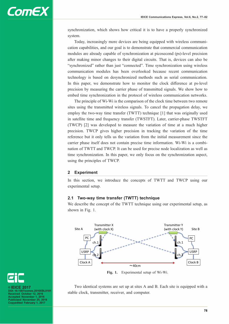
We describe the concept of the TWTT technique using our experimental setup, as

shown in Fig. 1.

Two identical systems are set up at sites A and B. Each site is equipped with a

stable clock, transmitter, receiver, and computer.

Fig. 1. Experimental setup of Wi-Wi.


78


In this paper, we denote time as T and the time interval as t. We denote the time

of clock A as TA and the time of clock B as TB. The difference between TA and TB,

tc � TB � TA, is calculated as follows.

Transmitter X at site A sends TTxA to site B. The receiver at site B receives the

signal at TRxB after a propagation delay, td. The time difference tB, between

reception at site B (TRxB) and transmission at site A (TTxA) is expressed as

tB � TRxB � TTxA ¼ tc þ td: ð1ÞTo cancel the propagation delay td, we also transmit TTxB to site A and record the

time difference from TRxA as tA:

tA � TRxA � TTxB ¼ �tc þ td: ð2ÞAssuming that variations in tc and td during the round trip of wireless communi-

cation are negligible, we subtract eq. (2) from eq. (1) and calculate tc as

tc ¼ tB � tA2

: ð3ÞThis is the basic concept of TWTT and has already been demonstrated in [1].

2.2 Carrier phase two-way time transfer (TWCP)

TWCP uses the carrier phase of the transmitted signal instead of the time signal.

Equation (3) can be rewritten using a measured phase,

tc � �c=ð4�f0Þ ¼ ð�B � �A þ 2�McÞ=ð4�f0Þ; ð4Þwhere f0 is the carrier frequency, �c is the phase difference between clocks A and

B, and �A is the phase advance of the transmitted signal after the propagation from

B to A. Likewise, �B is the phase advance of the transmitted signal after the

propagation from A to B. Since the measured phase can only be obtained as

modulo 2�, natural numberMc should be separately determined in order to measure

tc. One can, however, still measure tc repetitively, and the variation from the initial

measurement can be tracked when the variation of �c between adjacent measure-

ments is guaranteed to be smaller than π. This has already been demonstrated in [2].

2.3 TWCP using commercial transmitter

In this experiment, we used commercial, off-the-shelf transmitters for TWCP. These

transmitters are cheaper and users need not go through a cumbersome authorization

process to use them. However, since their internal clock is less stable than a

rubidium clock, they cannot be used to compare two rubidium clocks from two

remote sites in a simple manner. By measuring the phase of the same signal at

the transmitter as well as the receiver side and subtracting the phases, the trans-

mitter clock error can be cancelled. Using this technique, we were able to compare

the two rubidium clocks belonging to the two remote sites. The calculation method

is described in detail in the following sections.

2.4 Experimental setup

As shown in Fig. 1, each site consists of a personal computer (PC), a wireless

communication module, a software-defined radio with two receivers, and a rubi-

dium clock. We used a 2.4GHz ZigBee module (MoNoStick: Mono Wireless Inc.)


79


that was connected to the PC through a USB cable. The software-defined radios

(USRP-2942: National Instruments) were referenced to the 10MHz generated by

the rubidium clock (SIM940: Stanford Research Systems) through a coax cable.

The PC and USRP were connected by a PCI Express (PCIe) cable. We assigned

separate channels to each ZigBee module in the two locations for the sake of

simplicity. The USRP has two Rx channels: channel 1 received the signal from the

transmitter at the same site and channel 2 received the signal from the other site.

ZigBee communication is based on IEEE 802.15.4 (2450MHz) PHY, which

employs offset quadrature phase-shift keying (O-QPSK). The USRP digitizes the

baseband in-phase (I) and quadrature (Q) 16-bit signals at a rate of 4MSample/s

and sends them to the PC via the PCIe cable. The PC was used to decode the

signals, symbol by symbol, by taking the correlation of 16-chip sequences. The

phase was measured for each symbol and the average of all the unwrapped symbol

phases, representing the phase of each packet, was recorded.

2.5 Calculation procedure

The time sequence of Wi-Wi is illustrated in Fig. 2. Clocks X and Y are built into

the transmitters and are usually much less stable than a rubidium clock.

Commercially available wireless modules have a drawback that originates from

the fact that each wireless module has its own clock (clock X), and the transmitted

carrier phase is not easily synchronized with the clock of the transmitting site

(clock A). To eliminate the phase difference between clock X and clock A, the

carrier phase of the transmitted signal was measured at both sites. The difference

between the two measured phases reflects the phase difference between clocks A

and B. The phase of clock B with respect to clock A, �BðN Þ, was measured using

transmitter X, and the phase of clock A with respect to clock B, �AðN Þ, was

measured using transmitter Y as

Fig. 2. Time sequence of Wi-Wi.


80


�BðN Þ � �RxBðN Þ � �TxAðN Þ; ð5Þ�AðN Þ � �RxAðN Þ � �TxBðN Þ: ð6Þ

Here, �RxB denotes the phase of the clock X as received at site B and �TxA denotes

the phase of the clock X as received at site A. Similarly, �RxA denotes the phase

of the clock Y as received at site A and �TxB denotes the phase of clock Y

as received at site B. A and B denote the location of transmission or reception.

Although the phase of clock X and clock Y has no correlation with the rubidium

clocks due to its inaccuracy, �BðN Þ and �AðN Þ reflect the phase difference betweenclock A and B with the initial offset.

Finally, the time difference tc is calculated from eq. (4).

tcðN Þ � �cðN Þð4�f0Þ ¼

�BðN Þ � �AðN Þ þ 2�Mc

4�f0

; ð7Þ

This tc has ambiguity of Mc. By determining Mc by a separate technique, one can

calculate tc. Even if Mc is unknown, one can still unwrap the repetitive measure-

ment of phase to determine the variation of time from the beginning of the

measurement by keeping track of the change in Mc from the initial measurement.

2.6 Results

Fig. 3 shows the experimental results. We measured the clock variation over a

5min interval. Sites A and B are separated by about 40 cm. Transmitters X and Y

transmit the signals alternately at a rate of approximately 10 times per second.

Fig. 3 shows the case in which the antennae were stationary. The clock difference,

plotted in red, varied by about 2 ns over the 5min interval, which is reasonable for

rubidium clocks. The propagation delay, plotted in blue, varied by less than 10 ps

with a standard deviation of 2.2 ps. This 2.2 ps deviation indicates the measurement

limit of our 2.4GHz ZigBee Wi-Wi system. By connecting the same clock at the

two sites (clock A = clock B), we can directly determine the measurement noise of

tc, and we verified that the noise had the same deviation of 2 ps.

We used unwrapped º to calculate tc and td, as already mentioned in the

previous section. The unwrapping worked well because the variation between

adjacent measurements was much smaller than 0.4 ns which corresponds to 2� in

phase. The important point here is that since we use very stable clock for com-

parison, the measurement need not to be frequent. One measurement per second is

good enough with the rubidium clocks.

Fig. 3. Measurement of variation in clock difference and propagationdelay over a 5min interval using Wi-Wi.


81


3 Conclusion

We demonstrated that we can monitor the variation of the clocks and the prop-

agation delay of two remote communication devices by repeatedly measuring the

carrier phase of the transmitted signal. When the signal propagation environment is

favorable and the clocks are stable, Wi-Wi can achieve ps-level precision. Because

we used off-the-shelf transmitting devices, the licensing procedure is unnecessary.

Therefore, this setup is suitable for the research and development phase of

applications.

4 Outlook

Our technique should be immediately useful for the synchronization of two remote

clocks at ps level precision. Some of the applications of this technique include the

synchronization of wireless networks and smart grids, time-and position-tagged

data logging of sensors, and monitoring of the shape and tilt of buildings. In this

study, we used 2.4GHz ZigBee modules, but the concept of Wi-Wi can be easily

adapted to any wireless system which may employ various band and modulation

schemes.

Acknowledgments

This work was supported by the JST PRESTO program and NICT.


82


Underdetermined blindseparation of adjacentsatellite interference inmodern satellitecommunication systems

Chengjie Li1a), Lidong Zhu1b), and Zhen Zhang2c)1 National Key Laboratory of Science and Technology on Communication,

University of Electronic Science and Technology of China,

No. 2006, Xiyuan Ave, West Hi-Tech Zone, Chengdu, China2 NCS Pte. Ltd. of Singapore Telecommunications Limited,

Ang Mo Kio Street 62, NCS Hub, Singapore


b) [email protected]

c) [email protected]

Abstract: In this paper, a novel underdetermined blind source separation

algorithm guided by particle swarm optimizer (PSO) is proposed for adjacent

satellite interference in modern satellite communication systems. Different

from traditional methods, we formulate the separation problem as clustering

problem. Due to our algorithm is affected by the sparsity of source signals

and the density of mixed vectors, our algorithm is motivated by the

assumption is held that the distance between two arbitrary mixed signal

vectors is less than the doubled sum of variances of distribution of the

corresponding mixtures. In our method, we accomplish the underdetermined

blind source separation by computing the Short Time Fourier Transform

(STFT) to segment received mixtures and we use some estimates to separate

the mixed source signals by PSO where the number of the mixed signals is

unknown. In PSO, we define new parameters gather in formula (8) and cj in

formula (11). We verify the proposed method on several simulations. The

experimental results demonstrate the effectiveness of the proposed method.

Keywords: adjacent satellite interference, blind source separation, particle

swarm optimizer, Short Time Fourier Transform, sampling point

Classification: Fundamental Theories for Communications

References

[1] S. N. Livieratos, G. Ginis, and P. G. Cottis, “Availability and performance ofsatellite links suffering from interference by an adjacent satellite and rain fades,”IEE Proc., Commun., vol. 146, no. 1, pp. 61–67, 1999. DOI:10.1049/ip-com:19990285

[2] O. Tichý and V. Šmídl, “Bayesian blind separation and deconvolution of


83


http://dx.doi.org/10.1049/ip-com:19990285



dynamic image sequences using sparsity priors,” IEEE Trans. Med. Imaging,vol. 34, no. 1, pp. 258–266, Jan. 2015. DOI:10.1109/TMI.2014.2352791

[3] M. Atcheson, I. Jafari, R. Togneri, and S. Nordholm, “On the use of contextualtime-frequency information for full-band clustering-based convolutive blindsource separation,” IEEE International Conference on Acoustic, Speech andSignal Processing (ICASSP), pp. 2114–2118, 2014. DOI:10.1109/ICASSP.2014.6853972

[4] L. T. Duarte, J. M. T. Romano, C. Jutten, K. Y. Chumbimuni-Torres, and L. T.Kubota, “Application of blind source separation methods to ion-selectiveelectrode arrays in flow-injection analysis,” IEEE Sensors J., vol. 14, no. 7,pp. 2228–2229, 2014. DOI:10.1109/JSEN.2014.2318174

[5] M. A. Loghmari, M. S. Naceur, and M. R. Boussema, “A new sparse sourceseparation-based classification approach,” IEEE Trans. Geosci. Remote Sens.,vol. 52, no. 11, pp. 6924–6936, Nov. 2014. DOI:10.1109/TGRS.2014.2305724

[6] F. van den Bergh and A. P. Engelbrecht, “A cooperative approach to particleswarm optimization,” IEEE Trans. Evol. Comput., vol. 8, No. 3, pp. 225–239,June 2004. DOI:10.1109/TEVC.2004.826069

[7] T.-Y. Sun, C.-C. Liu, S.-J. Tsai, S.-T. Hsieh, and K.-Y. Li, “Cluster GuideParticle Swarm Optimization (CGPSO) for underdetermined blind sourceseparation with advanced conditions,” IEEE Trans. Evol. Comput., vol. 15,no. 6, pp. 798–811, Dec. 2011. DOI:10.1109/TEVC.2010.2049361

[8] C. C. Liu, T. Y. Sun, K. Y. Li, and S. T. Hsieh, and S. J. Tsai, “Blind sparsesource separation using cluster particle swarm optimization technique,” Proc.Int. Conf. Artif. Intell. Applicat., 549-217, 2007.

[9] Y. Ning, X. Zhu, S. Zhu, and Y. Zhang, “Surface EMG decomposition based onK-means clustering and convolution kernel compensation,” IEEE J. Biomed.Health Inform., vol. 19, no. 2, pp. 471–477, Mar. 2015. DOI:10.1109/JBHI.2014.2328497

1 Introduction

Adjacent satellite interference is same frequency interference caused by satellites in

nearby orbital location. Though people can reduce the influence by isolating wave

beam coverage area/frequency or reducing the antenna sidelobe etc., such cases of

interference happen more and more frequently due to synchronous orbit traffic get

heavier, especially for Ultra Small Apeture Terminal (USAT). Adjacent satellite

interference framework is shown in Fig. 1, the solid line is useful signal and

the dotted line is the adjacent satellite interference signal. For many years,

researches on adjacent satellite interference has been an important subject. In

1999, SLivieratos etc. adopted Crane model for adjacent interference of satellite

communication links [1].

Blind source separation (BSS) is a major research area in signal processing and

machine learning, and that has a large scope of applications in many fields, such as

image recognition, speech enhancement, biomedical signal processing, wireless

communications etc. [2, 3, 4] BSS aims to extract individual components from their

mixture samples where there is very limited, or no, prior information on mixture

samples nature or the mixing process. Recently, many BSS methods are based on

Independent Component Analysis with the assumption that the sources are inde-

pendent signals. However, if initial parameters are not given, those methods will


84


http://dx.doi.org/10.1109/TMI.2014.2352791




http://dx.doi.org/10.1109/ICASSP.2014.6853972




http://dx.doi.org/10.1109/JSEN.2014.2318174




http://dx.doi.org/10.1109/TGRS.2014.2305724




http://dx.doi.org/10.1109/TEVC.2004.826069








http://dx.doi.org/10.1109/JBHI.2014.2328497




produce a poor solution. And a suitable initial parameters is unlikely to be open

information because of the blind hypothesis. Consequently, some accurate, efficient

and robust BSS algorithms are desired.

We focus on BSS problem for adjacent satellite interference. To overcome the

above difficulties, this article proposes a novel particle swarm optimizer (PSO)

mechanism for identifying the exact mixing vector. In this article, we formulate

the separation problem as clustering problem. Due to our algorithm is affected by

the sparsity of source signals and the density of mixed vectors, our algorithm is

motivated by the fact that the assumption that the distance between two arbitrary

mixed signal vectors is less than the doubled sum of variances of distribution for

the corresponding mixtures is held.

The rest of this paper is organized as follows. In Section II, we introduce the

preparatory work of this article. In Section III, we introduce the novel BSS

algorithm with PSO. In Section IV, we introduce and discuss the experimental

results. Finally, the conclusion is drawn in Section V.

2 Preparatory work

In this section, we introduce the related preparatory work of Density Clustering

algorithm (DC-algorithm).

2.1 BSS model

BSS aims at separating a set of N unknown sources from a set of M observations.

Usually, the observations are obtained from M sensors, each sensor receives a

mixture of those sources. In this article, we only consider linear instantaneous

mixtures model, each observation is described as below [5]:

yjðtÞ ¼XNi¼1

aijsjðtÞ þ niðtÞ; j ¼ 1; 2; � � � ; M ð1Þ

Here, aij is the ði; jÞth element of the mixed matrix, niðtÞ is the ith component of the

noise. Equation (2) can also be written in matrix form,

YðtÞ ¼ ASðtÞ þ NðtÞ ð2Þ

Fig. 1. Framework of adjacent satellite interference


85


2.2 Particle swarm optimizer (PSO) model

In PSO, a goal is to minimize a objective function f, and there are three attributes,

the particles’ current position pi, current velocity vi, and local best position Pbi.

Each particle in the swarm is iteratively updated according to the aforementioned

attributes. In [6], a compact and workable PSO version is proposed, the new

velocity of every particle is updated by the following formula,

vijðg þ 1Þ ¼ �0 � vijðgÞ þ �1 � r1½PbijðgÞ � pijðgÞ�þ �2 � r2½GbjðgÞ � pijðgÞ�

ð3Þ

here, j ¼ 1; 2; . . . ; k denotes the index of dimension, i ¼ 1; 2; . . . ; sz denotes the

individual of particles, PbijðgÞ denotes the local best position of the jth dimension

of the ith particle, and GbjðgÞ denotes the global best position at the gth generation.

vijðgÞ is the velocity of the jth dimension of the ith particle. There are three

parameters that should be predefined suitably for the better performance of PSO.

�0 is the inertia weight of velocity, �1 and �2 denote the acceleration coefficients,

r1 and r2 are elements from two uniform random sequences in the range ð0; 1Þ, andg is the number of generations. The new position of a particle is calculated by the

following formula,

piðg þ 1Þ ¼ piðgÞ þ viðg þ 1Þ ð4ÞThe local best position of each particle is updated by

Pbiðg þ 1Þ ¼ PbiðgÞ; if fðpiðg þ 1ÞÞ � fðPbiðgÞÞpiðg þ 1Þ; otherwise

�ð5Þ

and the global best position (Gb) found from all particles during the previous three

steps is defined as

Gbðg þ 1Þ ¼ argminPbi

fðPbiðg þ 1ÞÞ; 1 � i � sz ð6Þ

The evolutionary process will continuously repeat (3)–(6) until some terminative

condition is reached.

3 Improved BSS algorithm with PSO

Because of only two sensors are available, the received mixtures are represented

as ½Y1ðt; fÞ; Y2ðt; fÞ�T . Since source signals are sparse, the mixtures center around

the mixing vectors on the Y1 � Y2 coordinate plane. And Yiðt; fÞ is described as

follows:

Yiðt; fÞ ¼Z 1

0

yðtÞhð� � tÞe�j2�f�d�; i ¼ 1; 2 ð7Þ

Here, yðtÞ is the received mixing signal, hð� � tÞ is the Hamming window function.

Thus, unobservable mixing vectors could emerge from these clusters of mixtures.

In fact, since local optima would reduce the performance of conventional methods

or the source signals may not be sparse enough, the mixing vectors not scattered

enough to be able to easily distinguished. In order to enhance BSS performance

and handle more advanced conditions, the improved BSS algorithm with PSO is

developed to search mixed vectors [7].© IEICE 2017DOI: 10.1587/comex.2016XBL0166Received September 13, 2016Accepted October 18, 2016Publicized November 30, 2016Copyedited February 1, 2017

86


3.1 Definition of parameter

In the development of BSS algorithm with PSO, p ¼ ½�1; �2; . . . ; �k� is a set of

estimated vectors and regarded as a particle of PSO, where 8� 2 ð� �2; �2Þ and k

denotes the dimension of each particle, that is, k is the maximal number of

estimated vectors. The elements of a particle represent the gathering angles of

mixtures. Since n mixing vectors have to be found and n is unknown, a value k

will be given, k � n. Compared with the [8], a normal angle with one dimension

replaced the original plane coordinate with two dimensions for some estimated

mixing vectors. Hence, the learning complexity can be reduced and the searching

range becomes definite.

Because the gathering directions of mixtures imply the location of the mixing

vectors, an objective function that evaluates how close the estimated mixing vectors

are to the gatherings is defined as

gather ¼XNi¼1

�2i � ��i ð8Þ

where �i ¼ffiffiffiffiffiffiffiffiffiffiffiffiffiffiffiffiffiffiffiffiffiffiffiffiy21ðiÞ þ y22ðiÞ

pdenotes the energy of the signal of the ith mixture, which

is regarded as the weight of each mixture. So, a sample with a large ξ indicates a

main signal that is regarded as important. ��i denotes the differential angle between

the ith mixture vector and the nearest estimated vector and is calculated by

��i ¼ minj�i � �jj; i ¼ 1:2; . . . ; N and j ¼ 1; 2; . . . ; k ð9Þwhere �i is the angle of the ith mixture vector. When all δ approach the center of

the mixture gathering, �� will reduce integrally. So, a particle responding with the

minimum of the objective function denotes its elements place exactly in the

direction of a gathering of mixtures. gather values of particles are evaluated by

(8). According to gather values we can update the Pb and Gb by (5) and (6).

3.2 Global best position Gb is replaced with cluster centers set CSince mixtures gather toward the mixing vectors, cluster centers are more likely to

produce a better solution than global best position (Gb). Moreover, it not only

substantially improves Gb during initial generations, but also fine tunes Gb during

final generations. Consequently, cluster information is the more preferable guide for

particles compared to Gb. The factor Gb is replaced with cluster centers set C in (7),

which could be rewritten as

vijðg þ 1Þ ¼ �0 � vijðgÞ þ �1 � r1½PbijðgÞ � pijðgÞ�þ �2 � r2½cjðgÞ � pijðgÞ�

ð10Þ

where fcjjj ¼ 1; 2; . . . ; kg 2 C is a set of cluster centers according to Gb, and each

component is evaluated by

cj ¼

Xcnji¼1

ð�2i � �iÞ

Xcnji¼1

�2i

ð11Þ


87


where j denotes the index of the cluster, cnj denotes the number of mixtures that

belong to the jth estimated vector, and i is the index of mixtures. Since the involved

signals are sparse, �i could be regarded as a weight to the angle of the ith mixture.

In other words, mixtures with a larger ξ have a greater effect upon the cluster center

that it belongs to, whereas others are noisy or even voiceless.

After the above process, the cluster centers can be found. Then, every remain-

ing sampling point is assigned to the same cluster as its nearest cluster center.

4 Simulation and blind source signal separation results

In this section, we verify the proposed method. In the simulation, the number of

source signals is three, the number of received signals is two. We aim to separate

the received mixed signals in time-frequency domain.

Each parameter is defined as follows: fb ¼ 2 � 105Hz for sample rate, Rb ¼103 bps for transmission bit rate, v ¼ 500 hop/s for hopping speed, f0 ¼ 2 � 103Hz

for modulation frequency, m ¼ 8 for bit numbers, the original signal numbers as

MK ¼ 3, and the receiving antenna numbers as RK ¼ 2.

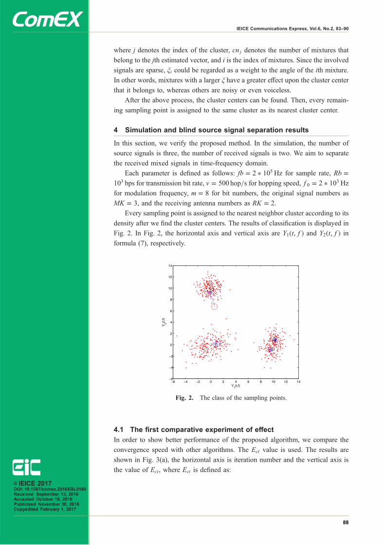
Every sampling point is assigned to the nearest neighbor cluster according to its

density after we find the cluster centers. The results of classification is displayed in

Fig. 2. In Fig. 2, the horizontal axis and vertical axis are Y1ðt; fÞ and Y2ðt; fÞ informula (7), respectively.

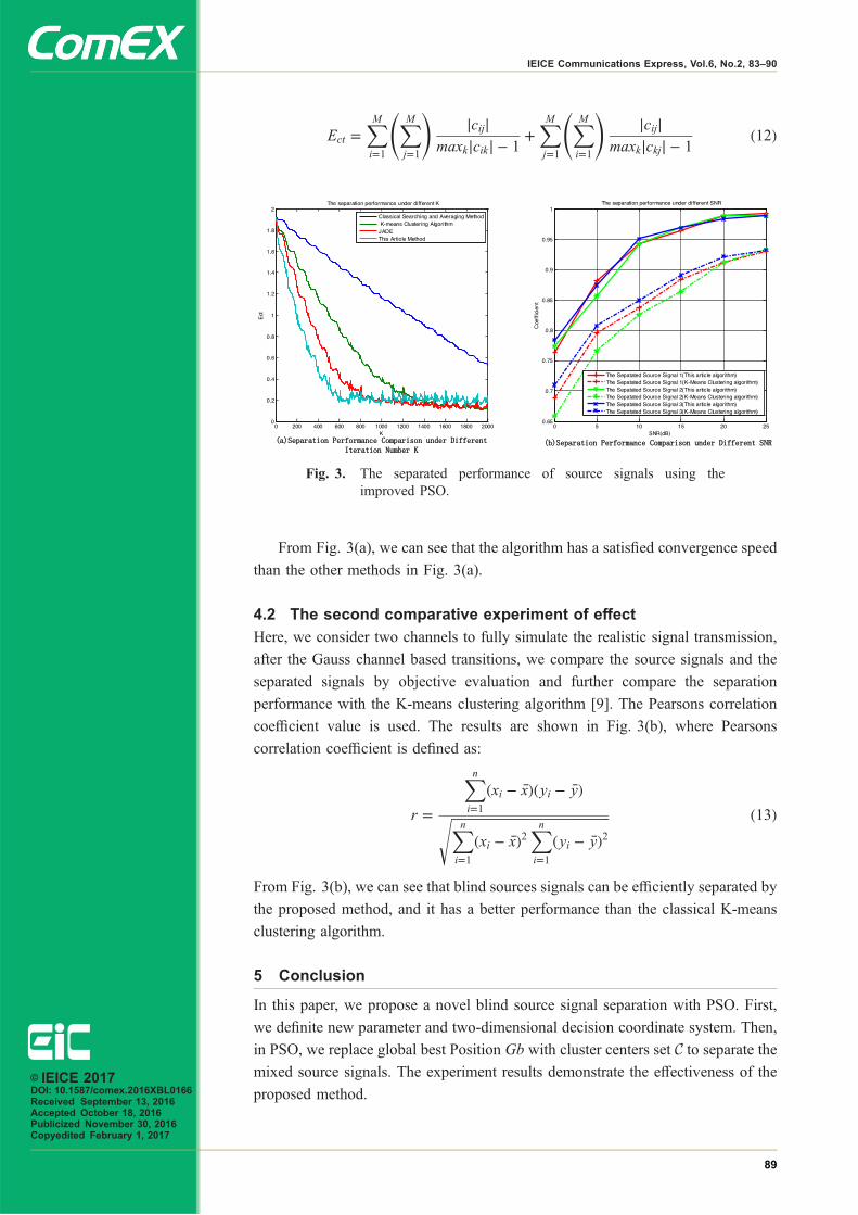
4.1 The first comparative experiment of effect

In order to show better performance of the proposed algorithm, we compare the

convergence speed with other algorithms. The Ect value is used. The results are

shown in Fig. 3(a), the horizontal axis is iteration number and the vertical axis is

the value of Ect, where Ect is defined as:

Fig. 2. The class of the sampling points.


88


Ect ¼XMi¼1

XMj¼1

!jcijj

maxkjcik j � 1þXMj¼1

XMi¼1

!jcijj

maxkjckjj � 1ð12Þ

From Fig. 3(a), we can see that the algorithm has a satisfied convergence speed

than the other methods in Fig. 3(a).

4.2 The second comparative experiment of effect

Here, we consider two channels to fully simulate the realistic signal transmission,

after the Gauss channel based transitions, we compare the source signals and the

separated signals by objective evaluation and further compare the separation

performance with the K-means clustering algorithm [9]. The Pearsons correlation

coefficient value is used. The results are shown in Fig. 3(b), where Pearsons

correlation coefficient is defined as:

r ¼

Xni¼1

ðxi � �xÞðyi � �yÞffiffiffiffiffiffiffiffiffiffiffiffiffiffiffiffiffiffiffiffiffiffiffiffiffiffiffiffiffiffiffiffiffiffiffiffiffiffiffiffiffiffiffiffiffiffiffiffiXni¼1

ðxi � �xÞ2Xni¼1

ðyi � �yÞ2s ð13Þ

From Fig. 3(b), we can see that blind sources signals can be efficiently separated by

the proposed method, and it has a better performance than the classical K-means

clustering algorithm.

5 Conclusion

In this paper, we propose a novel blind source signal separation with PSO. First,

we definite new parameter and two-dimensional decision coordinate system. Then,

in PSO, we replace global best Position Gb with cluster centers set C to separate the

mixed source signals. The experiment results demonstrate the effectiveness of the

proposed method.

Fig. 3. The separated performance of source signals using theimproved PSO.


89


Acknowledgments

This work is fully supported by a grant from the national High Technology

Research and development Program of China (863 Program) (No.

2012AA01A502), and National Natural Science Foundation of China

(No. 61179006), and Science and Technology Support Program of Sichuan

Province (No. 2014GZX0004).


90


Corrupted encoded datadetection for a CELP decoder

Hiroyuki Ehara1a), Takuya Kawashima2, and Toshiaki Sakurai11 Panasonic AVC Networks Company, Panasonic Corporation,

600 Saedo-cho, Tsuzuki-ku, Yokohama, Kanagawa 224–8539, Japan2 Panasonic System Networks R&D Lab. Co., Ltd.,

7F Confidence Kanazawa, 1–1–3 Sainen, Kanazawa, Ishikawa 920–0024, Japan


Abstract: Undetectable data corruption in wireless communication links

can occur in some cases, including cases in which a ciphering algorithm can

fail to generate the same keystream for encryption at a receiver side as it does

for a sender side. In wireless speech communication, such corruption might

trigger an explosion of decoded sound, which might in turn hurt a user’s ear.

This article presents a simple algorithm for detecting corruption for a typical

code-excited linear-prediction (CELP) speech decoder. The algorithm re-

quires no additional bits for corruption detection, but detects it by monitoring

the amplitude ratio of decoded adaptive and fixed excitation signals in CELP.

Its practicality is demonstrated by simulation.

Keywords: error detection, speech codec, CELP

Classification: Multimedia Systems for Communications

References

[1] 3GPP, “6.6.3 Ciphering method” in 3GPP TS 33.102 V12.2.0, p. 39, 2014.[2] N. Gortz, “Zero Redundancy Error Protection for CELP Speech Codecs,” Proc.

EuroSpeech’97, vol. 3, pp. 1283–1286, 1997.[3] M. R. Schroeder and B. S. Atal, “Code excited linear prediction: High quality

speech at low bit rates,” Proc. IEEE ICASSP-85, pp. 937–940, 1985. DOI:10.1109/ICASSP.1985.1168147

[4] J.-P. Adoul, P. Mabilleau, M. Delprat, and S. Morissette, “Fast CELP coding onalgebraic codes,” Proc. IEEE ICASSP-87, pp. 1957–1960, 1987. DOI:10.1109/ICASSP.1987.1169413

[5] T. Kawashima and H. Ehara, “Low bit-rate CELP decoder with corruptedencoded-data detection,” Proc. IEICE General Conference, D-14-18, Mar. 2016(in Japanese).

[6] P. J. Erdelsky, “Rijndael Encryption Algorithm,” http://www.efgh.com/software/rijndael.htm.

1 Introduction

In wireless communication systems, error protection is commonly applied to avoid

substantial degradation in communication quality caused by any error in commu-

nication links. However, in some cases, such errors are undetectable. For example,


91











http://www.efgh.com/software/rijndael.htm





some input parameters to a cipher algorithm can differ between the sender side and

the receiver side. Synchronization of an encryption keystream generated by the

cipher algorithm might be lost at the decoder side. This problem is known to occur

in some mobile communication systems using the ciphering method described in

3GPP specifications [1], which use sequence numbers counted separately at each

of the sender and receiver sides as input parameters. In this case, encoded data

received by a decoder are corrupted completely, but they are received as correct

encoded data. In speech communication systems, such corruption might trigger an

explosion of decoded sound, which might in turn hurt a user’s ear when headphone-

type listening devices are used. It is therefore desirable to detect such sound-

explosion-causing errors using corrupted data with no additional information.

An earlier study used the difference of consecutive decoded parameters for such

“zero-redundant” error detection [2]. This approach is based on the assumptions

that parameters decoded without error have some correlation in time, and that the

correlation diminishes if the data include errors. Errors can be detected by checking

whether the difference is outside of a predetermined range. A benefit of this

approach is that it enables parameter-by-parameter error detection, although some

wrong error detection is tolerated because the assumption is not always true. Our

objective is detecting corrupted data that might trigger an explosion of decoded

sound. We started with an investigation of the source of the sound explosion and

found that it was more appropriate for our objective to check excitation signals

reconstructed from the decoded parameters rather than the decoded parameters

themselves. By exploiting the excitation signals, we inferred a criterion that was

effective for detecting explosions. Using this criterion, we developed an algorithm

for corrupted encoded data detection (CED) used in a code-excited linear-prediction

(CELP) decoder. Its practicability is demonstrated by experimental simulation.

2 CELP decoder with corrupted encoded data detection

CELP [3], an algorithm for encoding speech signals at low bit-rates, is deployed

widely in wireless speech communication systems. It is based on a speech synthesis

model. Fig. 1 presents a block diagram of a CELP decoder with CED. After an

excitation signal is passed through a linear predictive synthesis filter, a synthesized

speech signal is outputted from the synthesis filter. Summing an adaptive codebook

(ACB) vector and a fixed-codebook (FCB) vector generates the excitation signal.

Fig. 1. Block diagram of a CELP decoder with CED.


92


The ACB, a buffered sequence of the excitation signal generated in the past, is used

to represent periodic components in the excitation signal. The FCB contains several

pre-fixed vectors. Such vectors can be represented in various ways. For example, in

widely deployed algebraic CELP (ACELP) [4], the pre-fixed vectors are generated

by combining some unit pulses located at pre-determined positions. The CED is

performed using both ACB and FCB vectors. Once the corrupted encoded data are

detected, attenuation is applied to the excitation signal input to the synthesis filter to

avoid explosion of synthesized sound [5]. The CED algorithm and the attenuation

of the excitation signal are explained herein in the following sections.

3 Criterion for detecting corrupted encoded data

The objective of this study is detecting corrupted encoded data for avoiding sound

explosion generation. Therefore, we have started with investigation of the sources

of sound explosions generated from corrupted encoded data. For generating

corrupted encoded data, an Advanced Encryption Standard (AES) cipher is used:

the Rijndael Encryption Algorithm [6]. A CELP-encoded bitstream is ciphered

using 256-bit AES. Then the ciphered bitstream is decrypted using a different

keystream from that used in encryption. The decrypted bitstream is then decoded by

the CELP decoder. Typical sound-explosion cases are selected and investigated

closely. Results show that the amplitude of the ACB vector (ACV) tends to be

remarkably large in those cases. However, a remarkable ACV amplitude is found

even in error-free conditions. Therefore, one cannot simply rely on the ACV

amplitude to detect sound-explosion cases. In our experience, the ratio between

the ACV amplitude and corresponding FCB vector (FCV) amplitude is useful as

a criterion for detecting abnormalities causing possible sound explosion. In CELP,

in general, the periodic component is represented with ACV. The non-periodic

component is represented with FCV. However, even if the input signal is a perfectly

periodic signal, FCV cannot be zero because a quantization error of the periodic

component always exists. Therefore, a practical upper limit of the ACV/FCV

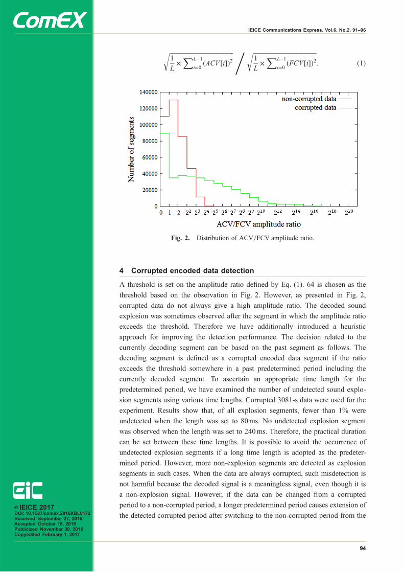
amplitude ratio must exist. We have examined the ACV/FCVamplitude ratio using

an approximately 3081-s database containing 8-language 800 short sentences with

no background noise, 8-language 80 short sentences with various background

noises (e.g. street noise, babble noise, car noise, train noise), 8-language 160 short

sentences at different input levels, and 13 music samples. Results show that the

ACB/FCB amplitude ratio never exceeds 50 for our developed CELP case.

However, when the corrupted encoded data are decoded, the ACV/FCV amplitude

ratio frequently exceeds 100. Fig. 2 presents histograms of the ACB/FCB ampli-

tude ratio for both cases. From Fig. 2, it is apparent that corrupted encoded data

segments are detectable by checking whether the ACV/FCV amplitude ratio

exceeds, for example, 64. Although the sound explosion is not always observed

in such cases, the amplitude ratio is useful as a reliable criterion for detecting the

corrupted encoded data. The amplitude ratio is defined by Eq. (1). ACV½i� and

FCV½i� respectively signify the decoded ACV and the decoded FCV, which are

scaled by corresponding quantized gains. L represents the vector length.© IEICE 2017DOI: 10.1587/comex.2016XBL0172Received September 27, 2016Accepted October 18, 2016Publicized November 30, 2016Copyedited February 1, 2017

93


ffiffiffiffiffiffiffiffiffiffiffiffiffiffiffiffiffiffiffiffiffiffiffiffiffiffiffiffiffiffiffiffiffiffiffiffiffiffiffiffiffi1

L�XL�1

i¼0 ðACV½i�Þ2

r , ffiffiffiffiffiffiffiffiffiffiffiffiffiffiffiffiffiffiffiffiffiffiffiffiffiffiffiffiffiffiffiffiffiffiffiffiffiffiffiffiffi1

L�XL�1

i¼0 ðFCV½i�Þ2

r: ð1Þ

4 Corrupted encoded data detection

A threshold is set on the amplitude ratio defined by Eq. (1). 64 is chosen as the

threshold based on the observation in Fig. 2. However, as presented in Fig. 2,

corrupted data do not always give a high amplitude ratio. The decoded sound

explosion was sometimes observed after the segment in which the amplitude ratio

exceeds the threshold. Therefore we have additionally introduced a heuristic

approach for improving the detection performance. The decision related to the

currently decoding segment can be based on the past segment as follows. The

decoding segment is defined as a corrupted encoded data segment if the ratio

exceeds the threshold somewhere in a past predetermined period including the

currently decoded segment. To ascertain an appropriate time length for the

predetermined period, we have examined the number of undetected sound explo-

sion segments using various time lengths. Corrupted 3081-s data were used for the

experiment. Results show that, of all explosion segments, fewer than 1% were

undetected when the length was set to 80ms. No undetected explosion segment

was observed when the length was set to 240ms. Therefore, the practical duration

can be set between these time lengths. It is possible to avoid the occurrence of

undetected explosion segments if a long time length is adopted as the predeter-

mined period. However, more non-explosion segments are detected as explosion

segments in such cases. When the data are always corrupted, such misdetection is

not harmful because the decoded signal is a meaningless signal, even though it is

a non-explosion signal. However, if the data can be changed from a corrupted

period to a non-corrupted period, a longer predetermined period causes extension of

the detected corrupted period after switching to the non-corrupted period from the

Fig. 2. Distribution of ACV/FCV amplitude ratio.


94


corrupted period. For consideration of such negative effects of detection perform-

ance, the F-measure was calculated for various time lengths for the predetermined

period using mixed data containing both non-corrupted and corrupted periods.

Corrupted data appear with 4 s intervals and have 2 s duration. Therefore, the

percentage of corrupted data is 50%. Again, the 3081-s data were used for

preparing mixed data. The F-measure was calculated using Eq. (2):

Recall ¼ correctly detected “corrupted segments”

actual “corrupted segments”

Precision ¼ correctly detected “corrupted segments”

detected “corrupted segments”: ð2Þ

F-measure ¼ 2 � Recall � Precision

Recall þ Precision

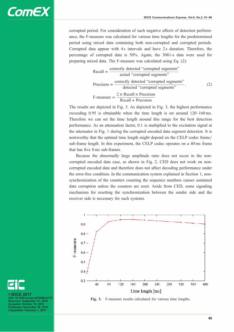
The results are depicted in Fig. 3. As depicted in Fig. 3, the highest performance

exceeding 0.95 is obtainable when the time length is set around 120–160ms.

Therefore we can set the time length around this range for the best detection

performance. As an attenuation factor, 0.1 is multiplied to the excitation signal at

the attenuator in Fig. 1 during the corrupted encoded data segment detection. It is

noteworthy that the optimal time length might depend on the CELP codec frame/

sub-frame length. In this experiment, the CELP codec operates on a 40ms frame

that has five 8ms sub-frames.

Because the abnormally large amplitude ratio does not occur in the non-

corrupted encoded data case, as shown in Fig. 2, CED does not work on non-

corrupted encoded data and therefore does not affect decoding performance under

the error-free condition. In the communication system explained in Section 1, non-

synchronization of the counters counting the sequence numbers causes sustained

data corruption unless the counters are reset. Aside from CED, some signaling

mechanism for resetting the synchronization between the sender side and the

receiver side is necessary for such systems.

Fig. 3. F-measure results calculated for various time lengths.© IEICE 2017DOI: 10.1587/comex.2016XBL0172Received September 27, 2016Accepted October 18, 2016Publicized November 30, 2016Copyedited February 1, 2017

95


5 Conclusion

This article proposes a detection algorithm using the amplitude ratio of adaptive-

codebook to fixed-codebook vectors in a code-excited linear prediction (CELP)

decoder for detecting corrupted encoded data segments without sending additional

information for error detection. The algorithm can apply to typical CELP-based

decoders without affecting the performance in an error-free condition. Moreover,

it can be integrated into an ordinary CELP decoding process without requiring a

specific signaling mechanism. It can therefore be introduced independently to any

decoder equipment without changing the entire communication system chain.


96


Decoupling stub-loadedparallel dipole array withorthogonal polarization

Kohei Omotea), Kazuhiro Honda, and Kun LiGraduate School of Engineering, Toyama University,

3190 Gofuku, Toyama-shi, Toyama 930–8555, Japan


Abstract: This paper presents a novel design for a two-element stub-loaded

dipole array antenna. The purpose is to obtain the decoupling and orthogonal

polarization characteristics using a small antenna configuration. A quarter-

wavelength stub loaded on one side of the two elements is operated as a

phase shifter to create the opposite phase of current distribution. Moreover,

the quarter-wavelength stub works as an orthogonal dipole antenna because

the in-phase currents are enhanced on the stub, leading to orthogonal

directivity. The results show that well-defined isolation and orthogonal

polarization directivity can be achieved using the proposed antenna.

Keywords: orthogonal polarization, decoupling, stub, dipole array

Classification: Antennas and Propagation

References

[1] D. Gesbert, M. Shafi, D. S. Shiu, P. J. Smith, and A. Naguib, “From theory topractice: An overview of MIMO space-time coded wireless systems,” IEEE J.Sel. Areas Commun., vol. 21, no. 3, pp. 281–302, Apr. 2003. DOI:10.1109/JSAC.2003.809458

[2] M. Nakano and H. Arai, “Orthogonal polarization base station antennatechnology at cellular systems and system evaluation,” IEICE Trans. Commun.,vol. J96-B, no. 1, pp. 1–15, Jan. 2013.

[3] D. T. Le, M. Shinozawa, and Y. Karasawa, “Wideband MIMO compact antennaswith tri-polarization,” IEICE Trans. Commun., vol. E94-B, no. 7, pp. 1982–1993, July 2011. DOI:10.1587/transcom.E94.B.1982

[4] K. Omote, H. Sato, K. Li, K. Honda, Y. Koyanagi, and K. Ogawa, “Three-axisdecoupling stub-loaded parallel dipole array with tri-orthogonal polarizationdirectivity,” IEEE iWEM 2015, Hsinchu, pp. 1–2, Nov. 2015. DOI:10.1109/iWEM.2015.7365037

[5] K. Nishizawa, H. Okegawa, H. Ohmine, Y. Sunahara, and T. Katagi, “A lineardipole antenna with crank sections suitable for an element operating at a lowerband in dual-band array antennas,” IEICE Trans. Commun., vol. J85-B, no. 6,pp. 932–940, June 2002.

[6] D. M. Pozar, Microwave Engineering, 3rd ed., p. 187, John Wiley & Sons,2005.

[7] FEKO, https://www.feko.info/.


97


http://dx.doi.org/10.1109/JSAC.2003.809458





http://dx.doi.org/10.1587/transcom.E94.B.1982





http://dx.doi.org/10.1109/iWEM.2015.7365037





https://www.feko.info/



1 Introduction

The multiple-input multiple-output (MIMO) technique was investigated to realize

ultra-high-speed and high-capacity mobile communications [1]. The polarized-

MIMO enhances the channel capacity more effectively compared with the space-

MIMO because of the low correlation between the antenna elements owing to space

orthogonality [2]. However, an orthogonally arranged antenna configuration is

disadvantageous for multi-element compactness because of its large size. There-

fore, miniaturizing the antenna is indispensable [3].

This paper presents a novel design for a two-element stub-loaded dipole array

antenna (SLDA). The feature of this proposal is that it realizes the orthogonal

polarization and decoupling characteristics simultaneously using a small antenna

configuration [4]. The current distribution on the stub generates the radiation

pattern using the common mode, whereas the nonradiation element of the stub-

loaded dipole produces well-defined isolation by using the opposite phase. The

analytical and measured results confirm that well-defined isolation and orthogonal

polarization directivity of SLDA can be achieved.

2 Operating principle of two-element stub-loaded dipole array

The stub structure is generally used to eliminate the undesired current component as

the parallel elements of the stub are nonradiation elements because of the opposite

phase mode [5]. We propose operating a stub as a radiation element with a common

mode in this paper in order to obtain orthogonal directivity.

Fig. 1 shows the operating principle of the two-element SLDA antenna for

realizing the orthogonal polarization and decoupling characteristics simultaneously.

Fig. 1(a) shows the current distribution of a two-element SLDA to illustrate the

orthogonal polarization directivity. The SLDA comprises two parallel dipole

antennas, in which one of the elements is loaded with a quarter-wavelength stub

for creating the opposite phase of the current distribution as a phase shifter.

When the stub-loaded element (Port 1) is excited, the opposite phase of the

current distribution is created with the same amplitude (I1 and �I1) on Element 1.

Thus, Element 1 is a nonradiation element because the currents cancel each other.

In this case, the radiation pattern is similar to that generated by a horizontal dipole

antenna because the in-phase currents I3 flowing on the Element Stub are enhanced

by each other. On the other hand, when the dipole element (Port 2) is excited, the

current of Element 2 (I2) is created. Consequently, the SLDA in Fig. 1(a) can be

treated as two orthogonally arranged dipoles, resulting in orthogonal polarization

directivity contributed by the current I3 on Element Stub and I2 on Element 2.

Fig. 1(b) shows the decoupling mechanism based on the current distribution of

the SLDA in Fig. 1(a). In Fig. 1(b), the separated dipole units on the right side

correspond to Element 1, whereas the single dipole on the left side represents

Element 2. Za12 and Zb

12 show the mutual impedance between Elements 1 and 2 in

the up-side and down-side, respectively.

Eqs. (1) and (2) show the matrices of the two dipoles (Element 1 and Ele-

ment 2) between the voltage V1 to V2, or �V1 to V2.© IEICE 2017DOI: 10.1587/comex.2016XBL0186Received October 19, 2016Accepted November 8, 2016Publicized November 30, 2016Copyedited February 1, 2017

98


V1

V2

" #¼

Za11 Za

12

Za21 Z22

" #I1

I2

" #ð1Þ

�V1

V2

" #¼ Zb

11 Zb12

Zb21 Z22

" # �I1I2

" #ð2Þ

Eq. (3) is obtained by transforming the plus and minus signs in Eq. (2).

V1

V2

" #¼ Zb

11 �Zb12

�Zb21 Z22

" #I1

I2

" #ð3Þ

The self-impedance and mutual impedance can be obtained by comparing

Eqs. (1) and (3) as shown below, respectively.

Zb11 ¼ Za

11 ð4ÞZb12 ¼ �Za

12 ð5ÞThe self-impedance in Eq. (4) has the same magnitude. The mutual impedance

in Eq. (5) has the same magnitude and opposite sign. Therefore, the total mutual

impedance ZT12 is zero, as expressed by the following equation.

ZT12 ¼ Za

12 þ Zb12 ¼ Za

12 � Za12 ¼ 0 ð6Þ

The isolation S12 depending on the Z parameter is defined in [6] as follows:

S12 ¼ 2ZT12Z0

ðZ11 þ Z0ÞðZ22 þ Z0Þ � ZT12Z

T21

ð7Þ

where Z0 is the load impedance, and Z11 and Z22 are the self-impedances. S12 can

be calculated as zero because ZT12 in Eq. (7) is zero, resulting in a high isolation in

theory.

The orthogonal polarization directivity and decoupling characteristics can be

simultaneously realized based on the two above-mentioned principles using two

linear elements instead of a complicated structure.

3 Design process of two-element stub-loaded dipole array

The simulation of a two-element SLDA was performed on the commercial EM

solver FEKO [7] based on the principles illustrated in Fig. 1. Fig. 2(a) shows the

Port 2

Port1 Element Stub

Element 1Element 2

I1

−I1

I2

I2

xy

zθ

φ

I3 Εφ

Εθ

I3

V2

V1

−V1

−+

I2

I2−+

−+

I1

I1

−I1

−I1bZ12

aZ12

22Z

aZ11

bZ11

(a) Current distribution (b) Decoupling mechanism

Fig. 1. Operating principle of two-element SLDA.


99


analytical model. It is designed to operate at a frequency of 2GHz. The length of

the dipole antenna is 7.5 cm (�=2 at 2GHz). The purpose of this simulation is to

determine the optimum dimension of the SLDA, including the stub length L and

element separation d, as shown in Fig. 2(a). The separation of Element Stub is

2mm. The element radius is 0.5mm.

Fig. 2(b) shows the isolation characteristics between Ports 1 and 2 for different

element separations d as a function of the phase difference. The phase difference

��, which depends on the stub length L, can be calculated by the following

equation.

�� ¼ 2L

�� 2� ð8Þ

In Fig. 2(b), the red, blue, and black lines show the cases in which the values of

element separation d are 5mm, 10mm, and 20mm, respectively.

In Fig. 2(b), the current flowing on the stub-loaded element has a distribution

opposite to that on the dipole element when the length of the stub is L ¼ �=4

(�� ¼ �), which is equal to that on an orthogonal dipole array antenna. Therefore,

an isolation greater than 30 dB can be achieved at 2GHz regardless of the antenna

separation d. As shown in Fig. 2(b), a high isolation of −32.5 dB is achieved when

the separation d is 5mm (0:03� at 2GHz).

On the other hand, the current flowing on the stub-loaded element has the same

distribution as that on the dipole element when L ¼ 0 (�� ¼ 0) or L ¼ �=2

(�� ¼ 2�), which equals that on the parallel dipole array antenna. Thus, the

currents of the two elements enhance each other, which eventually degrades the

isolation performance compared with that when L ¼ �=4.

The optimum dimension of the SLDA is determined at L ¼ �=4 and d ¼ 5mm

based on the simulation result shown in Fig. 2(b).

4 Measurement results

Fig. 3(a) shows the measurement setup of the two-element SLDA. As a preliminary

experiment, the dipole antenna with a feed structure of balun is used. Since the

balun is the additional part compared with the analytical model, they are orthog-

2mm

d

7.5cmL

Port 2 Port1x

y

zθ

φ

Element 1Element 2

Element Stub

d=λ/32=5mmd=λ/16=10mmd=λ/8=20mm

0 π 2π0 λ/4 λ/2

Δφ [rad]Length of Stub

S 21

[dB

]

(a) Antenna configuration (b) Isolation characteristics

Fig. 2. Design process of two-element stub-loaded dipole array.


100


onally-arranged along �x and �y-axis, respectively, in order to reduce the

undesired electromagnetic impact on radiation elements. The length of the stub is

3.75 cm (¼ �=4 at 2GHz). The element separation d between two elements is 5mm.

Fig. 3(b) shows the measured impedance characteristics of the SLDA. When

the specific port is excited, the other port is terminated with 50Ω. In Fig. 3(b), the

red line shows the result of the stub-loaded element (Port 1) and the blue line shows

that of the dipole (Port 2). As shown in Fig. 3(b), the impedance of Ports 1 and 2 at

Element 1Port1

Element 2Port2

x y

zθ

L=3.75cm

d=5mm

Balun

2mm 2GHz

1.8GHz

2.2GHz

2.2GHz

1.8GHz2GHz

Port2

Port1

Port1Port2

−26dB

−3dB

SLDA

dipole array

23dB

Solid Line: Measured ResultBroken Line: Analytical Result

zx-plane

EθEφ

Port 1

Port 2

f=2GHz

zy-plane xy-planez

z

z

z

x

x

y

y

x

x

y

y[dBd]

10

0

-10

-20

-10

0

10

[dBd]

10 0 -10 -20 -10 0 10

10 0 -10 -20 -10 0 1010

0

-10

-20

-10

0

10

(a) Measurement setup (b) Impedance characteristics

(c) S21 characteristics

(d) Orthogonal polarization directivity

Fig. 3. Measurement results of the proposed two-element stub-loadeddipole array.


101


2GHz is 79:4 þ j0:2Ω and 92:6 � j21:9Ω, respectively. Therefore, the VSWR of

the two elements are less than 2.5, indicating that there is no significant impedance

mismatch when the stub is loaded.

Fig. 3(c) shows the S21 characteristic of the SLDA. The red lines show the

proposed SLDA whereas the blue lines show the two-element vertical dipole array

designed at 2GHz. The solid and broken lines indicate the measured and analytical

results, respectively. As shown in Fig. 3(c), the SLDA can achieve an improvement

of 23 dB in the isolation at 2GHz compared with the result obtained using the

dipole array antenna.

Fig. 3(d) shows the radiation characteristics considering the mismatch loss. The

solid and broken lines indicate the measured and analytical results, respectively.

The blue line shows the E�-component and the red line indicates E�-component.

In Fig. 3(d), an eight-figure radiation pattern with the E�- and E�-components

in the zy- and xy-planes, respectively, can be observed when Port 1 is excited,

whereas an omnidirectional radiation pattern with the E�-component is obtained in

the zx-plane. Therefore, the radiation pattern of Port 1 is similar to a horizontal

dipole arranged along the y-axis. When Port 2 is excited, the radiation pattern is

similar to that of a vertical dipole arranged along the z-axis. These features indicate

that the proposed SLDA can realize the orthogonal polarization directivity.

In Fig. 3(d), the measurement results of the main polarization agree well with

the analytical results in all the planes. However, undesired polarization directivity

is observed. This phenomenon can be attributed to the electromagnetic coupling

between the element and the balun, and the radiation of the unnecessary current

caused by the difference in element length.

5 Conclusion

This paper presents a design example of two-element SLDA. The measured and

analytical results show that well-defined isolation and orthogonal polarization

directivity can be simultaneously realized with a small antenna configuration using

the proposed SLDA. As a future work, we are developing a practical antenna with

low-profile based on the design principle presented in this paper.


102


Temperature sensing usingan optical time domainreflectometer and mechanicallong-period fiber gratingsfabricated from a heat-shrinkable tube

Yasuhiro Tsutsumia), Masaharu Ohashi, and Yuji MiyoshiDepartment of Electrical and Information Systems, Graduate school of engineering,

Osaka Prefecture University, 1–1 Gakuen-cho, Naka Sakai, Osaka 599–8531, Japan


Abstract: We develop a simple temperature sensing using an optical time

domain reflectometer (OTDR) and a mechanical long-period fiber grating

(LPFG) fabricated from a heat-shrinkable tube and a metric screw. The

resonance loss of the fabricated LPFG is strongly dependent on temperature

as temperature-dependent heat-shrinkage of the tube produces a change in

the pressure applied to the fiber. In our proposed temperature sensor, the

LPFG insertion loss due to a change in the pressure applied to the fiber

is measured using an OTDR with a resonance wavelength. Both single-

point and multi-point temperature sensing is successfully demonstrated

experimentally.

Keywords: long period fiber gratings, optical time domain reflectometer,

temperature sensing

Classification: Sensing

References

[1] S. Nam, C. Zhan, J. Lee, C. Hahn, K. Reichard, P. Ruffin, K.-L. Deng, and S.Yin, “Bend-insensitive ultra short long-period gratings by the electric arcmethod and their applications to harsh environment sensing and communica-tion,” Opt. Express, vol. 13, pp. 731–737, 2005. DOI:10.1364/OPEX.13.000731

[2] H. Xuan, W. Jin, and M. Zhang, “CO2 laser induced long period gratings inoptical microfibers,” Opt. Express, vol. 17, pp. 21882–21890, 2009. DOI:10.1364/OE.17.021882

[3] S. W. James and R. P. Tatam, “Optical fibre long-period fiber grating sensors:characteristics and application,” Meas. Sci. Technol., vol. 14, no. 5, pp. R49–R61, 2003. DOI:10.1088/0957-0233/14/5/201

[4] V. Bhatia and A. M. Vengsarkar, “Optical fiber long-period fiber gratingsensors,” Opt. Lett., vol. 21, no. 9, pp. 692–694, 1996. DOI:10.1364/OL.21.000692

[5] Y. Wang, “Review of long period fiber gratings written by CO2 laser,” J. Appl.

© IEICE 2017DOI: 10.1587/comex.2016XBL0189Received October 31, 2016Accepted November 24, 2016Publicized December 8, 2016Copyedited February 1, 2017

103


http://dx.doi.org/10.1364/OPEX.13.000731




http://dx.doi.org/10.1364/OE.17.021882

http://dx.doi.org/10.1364/OE.17.021882

http://dx.doi.org/10.1364/OE.17.021882

http://dx.doi.org/10.1364/OE.17.021882

http://dx.doi.org/10.1088/0957-0233/14/5/201

http://dx.doi.org/10.1088/0957-0233/14/5/201

http://dx.doi.org/10.1364/OL.21.000692

http://dx.doi.org/10.1364/OL.21.000692

http://dx.doi.org/10.1364/OL.21.000692

http://dx.doi.org/10.1364/OL.21.000692

Phys., vol. 108, pp. 081101, 2010. DOI:10.1063/1.3493111[6] L. Drozin, P. Y. Fonjallaz, and L. Stensland, “Long-period fiber gratings written

by CO2 exposure of H2 loaded standard fibers,” Electron. Lett., vol. 36,pp. 742–744, 2000. DOI:10.1049/el:20000510

[7] G. Rego, O. Okhotnikov, E. Dianov, and V. Sulimov, “High-temperaturestability of long-period fibre gratings using an electric arc,” J. LightwaveTechnol., vol. 19, pp. 1574–1579, 2001. DOI:10.1109/50.956145

[8] P. Palai, M. N. Satyanarayan, M. Das, K. Thyagarajan, and B. P. Pal,“Characterization and simulation of long period gratings fabricated usingelectric discharge,” Opt. Commun., vol. 193, pp. 181–185, 2001. DOI:10.1016/S0030-4018(01)01231-7

[9] S. Savin, M. J. F. Digonnet, G. S. Kino, and H. J. Shaw, “Tunable mechanicallyinduced long-period fiber gratings,” Opt. Lett., vol. 25, pp. 710–712, 2000.DOI:10.1364/OL.25.000710

[10] H. Sakata and K. Yamashita, “Magnetic-force-induced long-period fibergratings,” Opt. Lett., vol. 37, pp. 1250–1252, 2012. DOI:10.1364/OL.37.001250

[11] Y. Tsutsumi, M. Ohashi, and Y. Miyoshi, “Temperature-sensitive mechanicalLPFG using contractive force of heat-shrinkable tube,” Opt. Fiber Technol.,vol. 19, pp. 55–59, 2013. DOI:10.1016/j.yofte.2012.11.002

[12] T. Erdogan, “Fiber grating spectra,” J. Lightwave Technol., vol. 15, no. 8,pp. 1277–1294, 1997. DOI:10.1109/50.618322

1 Introduction

A long-period fiber grating (LPFG) is formed in a single-mode fiber, which enables

light to be coupled from the fiber core to selected cladding modes at specific

resonance wavelengths. LPFGs have been extensively investigated for use in

optical communication and sensing applications because of their sensitivity to

strain, temperature, and refractive index [1, 2, 3].

Numerous techniques are available for fabricating LPFGs. Approaches that

have been demonstrated include periodic local heating of the fiber using a CO/CO2

laser [4, 5] or electric arc discharge [6, 7]. Fabrication techniques for mechanically

induced LPFGs have also been reported [8, 9, 10]. Mechanically induced LPFGs

are attractive because of their simplicity, flexibility, and cost effectiveness. In a

recent paper, we proposed a new mechanically induced LPFG fabricated from a

heat-shrinkable tube and a metric screw and reported its temperature characteristics

[11].

In the current study, we propose a simple temperature-sensing using an optical

time domain reflectometer (OTDR) and an LPFG fabricated from a heat-shrinkable

tube and a metric screw. In the proposed sensing, the OTDR senses the temperature

from the LPFG insertion loss that occurs when pressure is applied to the fiber. We

demonstrate successfully both single-point and multi-point temperature sensing.

2 Temperature sensing using an OTDR and LPFG

Fig. 1 shows the temperature measurement configuration. Temperature sensing is

achieved by monitoring the insertion loss at a wavelength near the resonance

wavelength of the LPFG. The transmitted spectrum changes significantly in line


104


http://dx.doi.org/10.1063/1.3493111

http://dx.doi.org/10.1063/1.3493111

http://dx.doi.org/10.1063/1.3493111

http://dx.doi.org/10.1049/el:20000510

http://dx.doi.org/10.1049/el:20000510

http://dx.doi.org/10.1109/50.956145

http://dx.doi.org/10.1109/50.956145

http://dx.doi.org/10.1109/50.956145

http://dx.doi.org/10.1016/S0030-4018(01)01231-7

http://dx.doi.org/10.1016/S0030-4018(01)01231-7

http://dx.doi.org/10.1364/OL.25.000710

http://dx.doi.org/10.1364/OL.25.000710

http://dx.doi.org/10.1364/OL.25.000710

http://dx.doi.org/10.1364/OL.25.000710

http://dx.doi.org/10.1364/OL.37.001250

http://dx.doi.org/10.1364/OL.37.001250

http://dx.doi.org/10.1364/OL.37.001250

http://dx.doi.org/10.1364/OL.37.001250

http://dx.doi.org/10.1016/j.yofte.2012.11.002






http://dx.doi.org/10.1109/50.618322

http://dx.doi.org/10.1109/50.618322

http://dx.doi.org/10.1109/50.618322

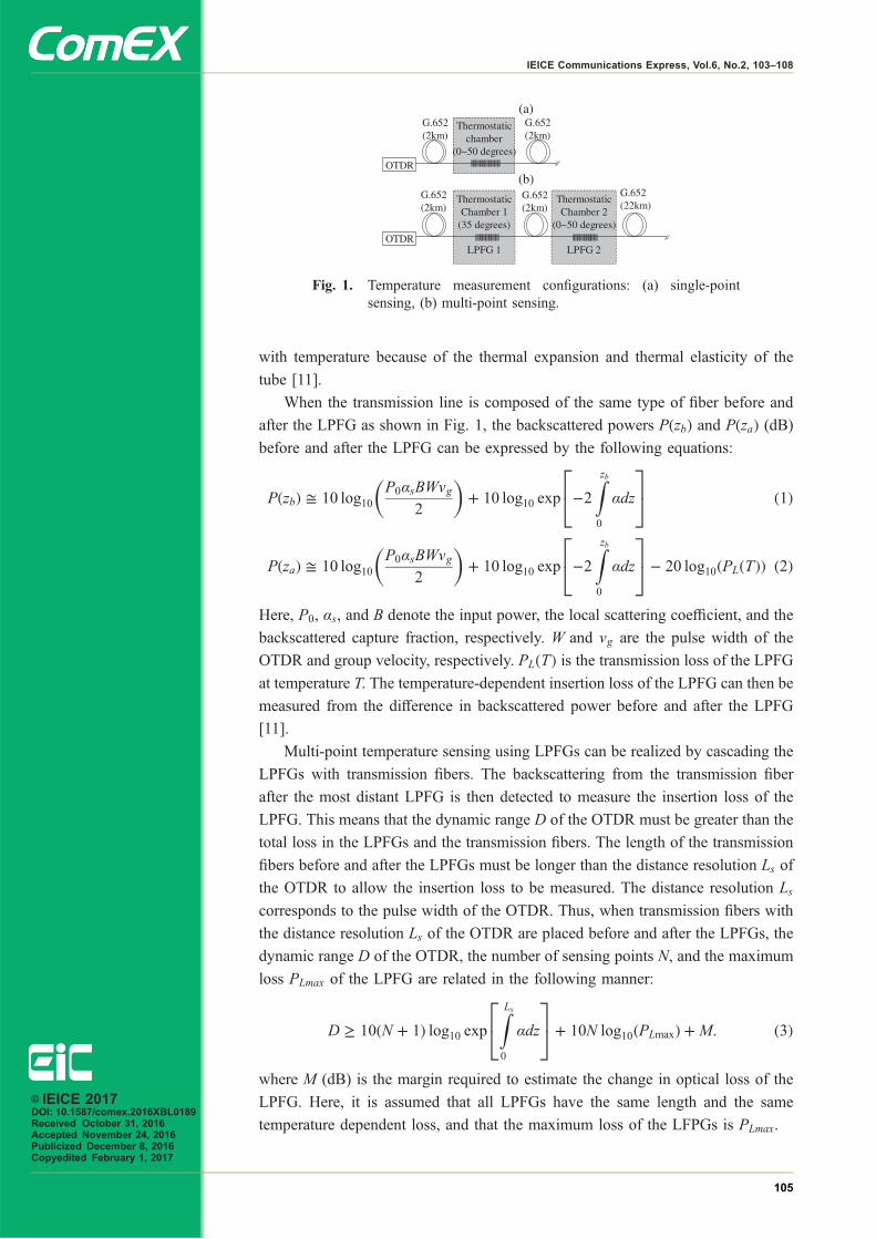
with temperature because of the thermal expansion and thermal elasticity of the

tube [11].

When the transmission line is composed of the same type of fiber before and

after the LPFG as shown in Fig. 1, the backscattered powers PðzbÞ and PðzaÞ (dB)before and after the LPFG can be expressed by the following equations:

PðzbÞ ffi 10 log10P0�sBWvg

2

� �þ 10 log10 exp �2

Zzb0

�dz

24

35 ð1Þ

PðzaÞ ffi 10 log10P0�sBWvg

2

� �þ 10 log10 exp �2

Zzb0

�dz

24

35 � 20 log10ðPLðTÞÞ ð2Þ

Here, P0, �s, and B denote the input power, the local scattering coefficient, and the

backscattered capture fraction, respectively. W and vg are the pulse width of the

OTDR and group velocity, respectively. PLðTÞ is the transmission loss of the LPFG

at temperature T. The temperature-dependent insertion loss of the LPFG can then be

measured from the difference in backscattered power before and after the LPFG

[11].

Multi-point temperature sensing using LPFGs can be realized by cascading the

LPFGs with transmission fibers. The backscattering from the transmission fiber

after the most distant LPFG is then detected to measure the insertion loss of the

LPFG. This means that the dynamic range D of the OTDR must be greater than the

total loss in the LPFGs and the transmission fibers. The length of the transmission

fibers before and after the LPFGs must be longer than the distance resolution Ls of

the OTDR to allow the insertion loss to be measured. The distance resolution Ls

corresponds to the pulse width of the OTDR. Thus, when transmission fibers with

the distance resolution Ls of the OTDR are placed before and after the LPFGs, the

dynamic range D of the OTDR, the number of sensing points N, and the maximum

loss PLmax of the LPFG are related in the following manner:

D � 10ðN þ 1Þ log10 expZLs0

�dz

24

35 þ 10N log10ðPLmaxÞ þM: ð3Þ

where M (dB) is the margin required to estimate the change in optical loss of the

LPFG. Here, it is assumed that all LPFGs have the same length and the same

temperature dependent loss, and that the maximum loss of the LFPGs is PLmax.

(a)

(b)

Fig. 1. Temperature measurement configurations: (a) single-pointsensing, (b) multi-point sensing.


105


The optical loss of the LPFG fabricated from a heat-shrinkable tube and a

metric screw comprises losses caused by periodic refractive index modulation and

by random microbending [11]. The microbending loss is negligible compared with

the loss from periodic refractive index modulation [11]. Thus, the optical loss PL at

the resonance wavelength of the LPFG can be expressed as follows [12]:

PL ffi sin2ð� lÞ: ð4Þwhere κ and l are the coupling coefficient and the length of the LPFG, respectively.

The design of the LPFG sensor was based on Eqs. (3) and (4).

Next, we describe how the number of sensors and the distance range for

multipoint sensing were determined. When the pulse width of the OTDR was set to

1 µs, Ls was found to be 0.1 km. We assumed the maximum loss PLmax of the LPFG,

the dynamic range of the OTDR, the optical loss of the fiber, and the margin M to

be 1.4 dB, 32 dB, 0.2 dB/km, and 15 dB, respectively. From Eq. (3), the maximum

number of sensing points N was found to be 11. The sensing distance range was,

therefore, 2.2 km (0:2 � 11).

3 Experimental results

Fig. 1(a) shows the experimental setup used to measure the insertion loss of the

LPFG at the temperature T. We used a commercially available metric screw (M3)

with a pitch Λ of 500µm, a length of 5 cm, and a diameter of 3mm. An LPFG was

spliced between two optical fiber bobbins with a fiber length of 2 km (ITU-T G.652

fibers), and placed in a thermostatic chamber. The temperature was then changed

from 0 to 50 °C. An OTDR (Agilent E6003C) was used to derive the LPFG

insertion loss 10 log10ðPLÞ (dB) from the backscattered power distribution. The

OTDR wavelength was set at 1,555 nm while taking the resonance wavelength of

the LPFG into account. The averaging time was 10 s and the pulse width was

300 ns, corresponding to a spatial resolution of 30m.

Fig. 2(a) shows the temperature dependence of the backscattered power dis-

tributions of the fiber link containing the LPFG. It can be seen that the back-

scattered power after the LPFG changed as the temperature in the thermostatic

chamber changed. The backscattered power variation before and after the LPFG,

corresponding to the insertion loss, was dependent on the temperature. This is

because the resonance loss is also temperature dependent [11].

Fig. 3(a) shows the relationship between the natural logarithm of the insertion

loss lnð10 log10ðPLÞÞ of the LPFG and the temperature T. The insertion loss of the

LPFG fabricated from a heat-shrinkable tube showed a good fit with the exponen-

tial temperature function [11]. We, therefore, calculated the natural logarithm of

the insertion loss. The open and filled circles show the insertion loss of the LPFG in

the heating and cooling cycles, respectively. Measurements were taken three times

in each cycle. The solid line was linearly fitted to the experimental data, measured

in the heating cycle. It can be seen that the natural logarithm of the LPFG insertion

loss decreased in direct proportion to the temperature. The experimental temper-

ature dependence of the insertion loss PL can be expressed as follows:

lnð10 log10ðPLÞÞ ¼ �0:0452 T þ 0:160 ð5Þ© IEICE 2017DOI: 10.1587/comex.2016XBL0189Received October 31, 2016Accepted November 24, 2016Publicized December 8, 2016Copyedited February 1, 2017

106


This allows the temperature T to be estimated from the natural logarithm of the

insertion loss. The temperature in the thermostatic chamber was estimated from the

insertion loss using Eq. (5), as shown in Fig. 2(a).

The temperature T was obtained as follows:

T ¼ ð0:160 � lnð10 log10ðPLÞÞÞ=0:0452 ð6ÞWe defined the estimated temperature difference as the difference between the

temperature in the thermostatic chamber and the estimated temperature obtained

by substituting the measured insertion loss into Eq. (6). Across six measurements,

the difference between the measured and estimated temperature was within 2 °C.

(a)

(b)

Fig. 2. Backscattered power distribution of the fiber link: (a) single-point sensing, (b) multi-point sensing.

(a)

(b)

Fig. 3. Natural logarithm of insertion losses of LPFGs: (a) single-pointsensing, (b) multi-point sensing.


107


To investigate multi-point sensing, the temperatures of a fiber link comprising

two LPFGs (LPFG1 and LPFG2) were measured, as shown in Fig. 1(b). The

lengths of LPFG1 and LPFG2 were 5.3 cm and 4.0 cm, respectively. Both were

placed in thermostatic chambers. LPFG1 was kept at a constant 35 °C, while

LPFG2 was heated from 0 to 50 °C. The backscattered power distribution was

measured at the different temperatures of LPFG2 using the OTDR at a pulse width

of 1 µs and an averaging time of 10 s.

Fig. 2(b) shows the backscattered power distributions of the fiber link contain-

ing the two LPFGs. The backscattered power difference before and after LPFG1

was almost unchanged because the temperature was kept constant. By contrast, the

backscattered power difference before and after LPFG2 decreased as the temper-

ature increased.

Fig. 3(b) shows the natural logarithm of the insertion losses of LPFG1 and

LPFG2. Dots represent the natural logarithm of the insertion loss of LPFG1, at

constant temperature, and the open circles represent that of LPFG2, at temperatures

ranging from 0 to 50 °C. It can be seen that the insertion loss of LPFG1 was almost

unchanged, whereas the insertion loss of LPFG2 changed in line with the temper-

ature. This confirmed that the maximum loss of the LPFG could be varied by

changing the length of the LPFG. The difference between the measured temperature

in thermostatic chamber 2 and the estimated temperature was within 2 °C, and the

experimental results showed good repeatability. This confirmed that the estimation

of temperature distributions was possible using our proposed method.

4 Conclusions

We have proposed a simple and cost-effective temperature sensing based on a

mechanical LPFG fabricated from a heat-shrinkable tube and a metric screw, both

of which are commercially available. We have confirmed that the insertion loss of

the LPFG measured using a conventional OTDR is temperature dependent. Our

proposed technique has been used to measure the temperature of a thermostatic

chamber with an accuracy of 2 °C. Multi-point temperature sensing has then been

investigated, using two LPFGs. As in the single-point temperature measurement

experiment, the accuracy has been found to be within 2 °C. The experimental

results have confirmed the potential use of LPFGs for temperature sensing.

Acknowledgments

The authors would like to thank Dr. I. Yamashita at the Kansai Electric Power Co.,

Inc. for a fruitful discussion and providing us with the thermostatic chamber. This

work was supported by JSPS KAKENHI Grant Number 16K06307.


108


ieice communications express, vol.6, no.2, 65 low ... letter assumes a dl-mu-mimo-ofdm system in...

Documents