ifcam kick-off meeting university of nice, 19-21 novenber, 2012
TRANSCRIPT

IFCAMKick-off meeting
University of Nice,19-21 Novenber, 2012
Control ofCompressible Navier Stokes System
Mythily RamaswamyTIFR Centre for Applicable Mathematics, Bangalore, India
Mythily Ramaswamy () 21st November, 2012 1 / 26

T.I.F.R Center for Applicable Mathematics
TIFR Centre for Applicable Mathematics, Bangalore
Mythily Ramaswamy () 21st November, 2012 2 / 26

Collaborators and Support
Collaborators:
Jean-Pierre Raymond (IMT, Toulouse),
Shirshendu Chowdhury, Debayan Maiti, Debanjana Mitra (TIFR-CAM)
Financial Support :
Indo-French Center for Promotion of Advanced Research, New Delhi
Project : IFC 3701-1
Mythily Ramaswamy () 21st November, 2012 3 / 26

Introduction Compressible Navier Stokes System in 1D
Compressible Navier Stokes System in 1D
The Navier-Stokes system for viscous compressible fluid in an interval of Rfor density ρ(x, t) and velocity v(x, t) for x ∈ R, t > 0
ρt(x, t) + (ρv)x(x, t) = 0,
ρ(x, t)[vt(x, t) + v(x, t)vx(x, t)] + (p(ρ))x(x, t) − νvxx(x, t) = 0,(1)
ν > 0 is the fluid viscosity;p, the pressure satisfies the constitutive law
p(ρ) = a ργ for a > 0, γ ≥ 1. (2)
Mythily Ramaswamy () 21st November, 2012 4 / 26

Introduction Scope of our work
Scope of our work
Linearize the system around constant steady states
With suitable boundary conditions get the spectrum and and aFourier basis
Study controllability : interior and boundary null controllability andapproximate controllabilty
Study stabilizability
Using this study local stabilizability of the nonlinear system
Mythily Ramaswamy () 21st November, 2012 5 / 26
Introduction Scope of our work
Known Results
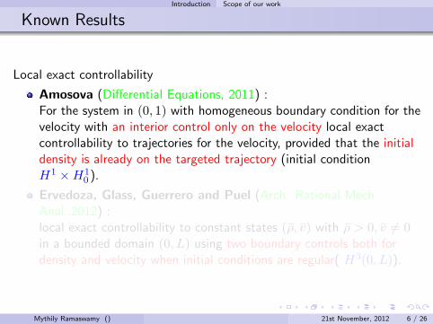
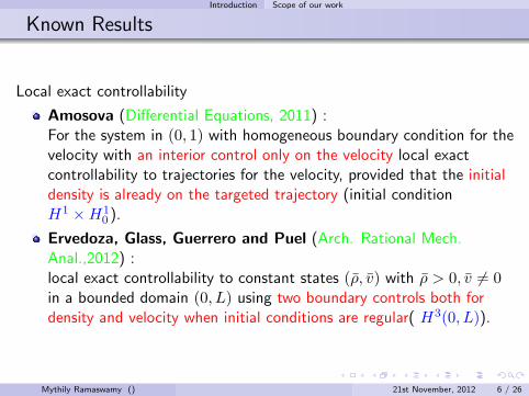
Local exact controllability
Amosova (Differential Equations, 2011) :For the system in (0, 1) with homogeneous boundary condition for thevelocity with an interior control only on the velocity local exactcontrollability to trajectories for the velocity, provided that the initialdensity is already on the targeted trajectory (initial conditionH1 ×H1
0 ).
Ervedoza, Glass, Guerrero and Puel (Arch. Rational Mech.Anal.,2012) :local exact controllability to constant states (ρ, v) with ρ > 0, v 6= 0in a bounded domain (0, L) using two boundary controls both fordensity and velocity when initial conditions are regular( H3(0, L)).
Mythily Ramaswamy () 21st November, 2012 6 / 26
Introduction Scope of our work
Known Results
Local exact controllability
Amosova (Differential Equations, 2011) :For the system in (0, 1) with homogeneous boundary condition for thevelocity with an interior control only on the velocity local exactcontrollability to trajectories for the velocity, provided that the initialdensity is already on the targeted trajectory (initial conditionH1 ×H1
0 ).
Ervedoza, Glass, Guerrero and Puel (Arch. Rational Mech.Anal.,2012) :local exact controllability to constant states (ρ, v) with ρ > 0, v 6= 0in a bounded domain (0, L) using two boundary controls both fordensity and velocity when initial conditions are regular( H3(0, L)).
Mythily Ramaswamy () 21st November, 2012 6 / 26

Introduction Linearization
Initial boundary value problem for the linearized system
Domain Ω = (0, π)(Q0, v0) : a constant steady state solution with Q0 > 0, v0 ≥ 0Linearized system around this solution :
∂tρ + v0ρx + Q0 ux = 0
∂tu − ν
Q0uxx + v0 ux + aγ Qγ−2
0 ρx = fχO
with O ⊂ ΩInitial, boundary conditions :
ρ(x, 0) = ρ0(x) ; u(x, 0) = u0(x),u(0, t) = q0(t) ; u(π, t) = q1(t) ∀ t > 0
Additional boundary conditions for ρ wherever v0 > 0Distributed (internal) control : f ; Boundary controls q0, q1
Mythily Ramaswamy () 21st November, 2012 7 / 26

Linearization around (Q0, 0)
Function space framework
Function space for the case v0 = 0 : Z = L2(Ω) × L2(Ω)Equip with innerproduct⟨(
ρu
),
(σv
)⟩z
= aγQγ−20
∫ π
0ρ(x)σ(x)dx+Q0
∫ π
0u(x)v(x)dx
A dense subspace :
D(A) = (ρ(x)u(x)
)∈ Z : u(x) ∈ H1
0 (Ω), (bρ(x)− cu′(x)) ∈ H1(Ω)
Define A : D(A)→ Z :
A =
[0 Q0
ddx
aγQγ−20
ddx
−νQ0
d2
dx2
]D(A) is dense in Z ; A is maximal monotone
(−A,D(A)) is the infinitesimal generator of C0 semigroup S(t) on Z.
Mythily Ramaswamy () 21st November, 2012 8 / 26

Linearization around (Q0, 0)
Operator Equation
Call U(x, t) =(ρ(x, t)u(x, t)
)System without controls :
dU(t)dt
+ AU(t) = 0, t > 0
U(0) = U0 ∈ Z.
For every U0 ∈ Z, there is a unique solution U in C([0,∞),Z)
Mythily Ramaswamy () 21st November, 2012 9 / 26
Linearization around (Q0, 0) Existence via semigroup theory
Spectrum of A when v0 = 0
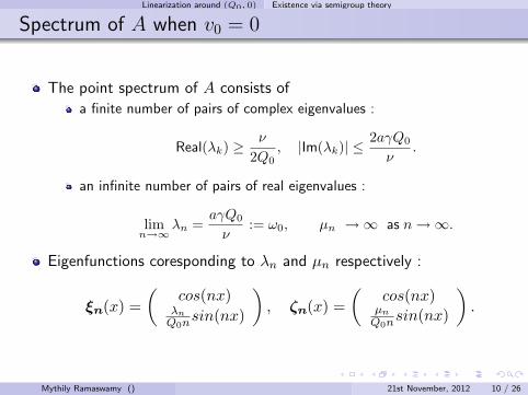
The point spectrum of A consists of
a finite number of pairs of complex eigenvalues :
Real(λk) ≥ ν
2Q0, |Im(λk)| ≤ 2aγQ0
ν.
an infinite number of pairs of real eigenvalues :
limn→∞
λn =aγQ0
ν:= ω0, µn →∞ as n→∞.
Eigenfunctions coresponding to λn and µn respectively :
ξn(x) =(
cos(nx)λnQ0n
sin(nx)
), ζn(x) =
(cos(nx)µnQ0n
sin(nx)
).
Mythily Ramaswamy () 21st November, 2012 10 / 26
Linearization around (Q0, 0) Spectral analysis
Orthonormal basis
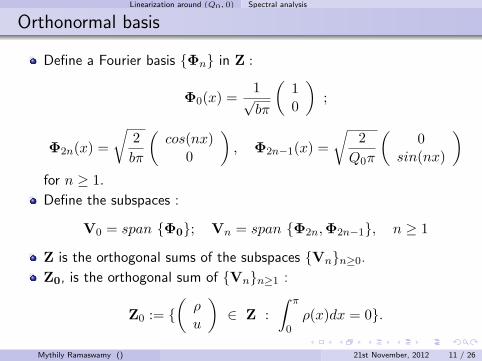
Define a Fourier basis Φn in Z :
Φ0(x) =1√bπ
(10
);
Φ2n(x) =
√2bπ
(cos(nx)
0
), Φ2n−1(x) =
√2
Q0π
(0
sin(nx)
)for n ≥ 1.Define the subspaces :
V0 = span Φ0; Vn = span Φ2n,Φ2n−1, n ≥ 1
Z is the orthogonal sums of the subspaces Vnn≥0.
Z0, is the orthogonal sum of Vnn≥1 :
Z0 := (ρu
)∈ Z :
∫ π
0ρ(x)dx = 0.
Mythily Ramaswamy () 21st November, 2012 11 / 26

Linearization around (Q0, 0) Controllability of Linearized CNS System
Interior control
Qn : Can we bring the linearized system to rest in time T bycontrolling the velocity in Ω ?
The system :
U(t) +AU(t) = F(t)U(0) = U0
F(t) =(
0f(., t)
), f ∈ L2((0,∞), L2(Ω))
Using the Fourier basis in Z0,
F(t) =∞∑n=1
fn(t)Φ2n−1.
Mythily Ramaswamy () 21st November, 2012 12 / 26

Linearization around (Q0, 0) Controllability of Linearized CNS System
Controllability
When a basis is available, one can try building a control :
Project the system on finite dimensional spaces
If the finite dimensional system is controllable, find a minimum normcontrol
Sum up these finite dimensional control to build a control for the fullspace
Mythily Ramaswamy () 21st November, 2012 13 / 26

Linearization around (Q0, 0) Controllability of Linearized CNS System
Projected system
The system projected on Vn is
Un(t) +AnUn(t) = pn(t)B, B =[
01
]Un(0) = U0,n
Un = U |Vn and U0,n = U(0) |Vn .
For any given T > 0, the finite dimensional system is controllable.
Using optimal control theory, can find minimal norm control :
fn(t) = −(B∗e−(T−t)A∗nW−1T e−TAn)U0,n,
WT =
T∫0
e−tAnBB∗e−tA∗ndt
Mythily Ramaswamy () 21st November, 2012 14 / 26
Linearization around (Q0, 0) Controllability of Linearized CNS System
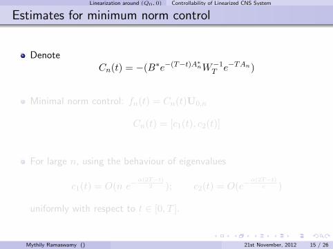
Estimates for minimum norm control
DenoteCn(t) = −(B∗e−(T−t)A∗nW−1
T e−TAn)
Minimal norm control: fn(t) = Cn(t)U0,n
Cn(t) = [c1(t), c2(t)]
For large n, using the behaviour of eigenvalues
c1(t) = O(n e−α(2T−t)
2 ); c2(t) = O(e−α(2T−t)
c )
uniformly with respect to t ∈ [0, T ].
Mythily Ramaswamy () 21st November, 2012 15 / 26

Linearization around (Q0, 0) Controllability of Linearized CNS System
Null controllability
f ∈ L2((0,∞), L2(Ω)) iff∑‖fn‖2L2(0,∞) <∞, iff∑∞n=1
∫ π0 |c1(t)U1
0,n + c2(t)U20,n|2dt < ∞
if and only if the initial value U0 ∈ H1m(Ω)× L2(Ω) .
Theorem
For T > 0, the system is null controllable in time T , using interior control
f ∈ L2((0,∞), L2(Ω)) if and only if U0 =(ρ0
u0
)∈ H1
m(Ω)× L2(Ω),
H1m(Ω) = ρ ∈ H1(Ω) :
∫ π0 ρ(x)dx = 0.
This is optimal in the sense that the system is not null controllable usingany boundary control or an interior control acting on a subset of Ω.
Mythily Ramaswamy () 21st November, 2012 16 / 26

Linearization at (Q0, v0)
Linearized system at (Q0, v0)
For the linearized system around (Q0, v0) withPeriodic boundary conditions for ρ, u and ux in (0, 2π)
The spectrum lies on the left side of the complex plane, infinite number oftwo pairs of complex eigenvalues and no accumulation point in thespectrum. Absolute value of the eigenvalues goes to infinity.Can work with Fourier basis and Moment method.
ResultsApproximately controllable for T sufficiently large.Null controllable with regular interior control and also regular boundarycontrol if T > 2π
v0.
Mythily Ramaswamy () 21st November, 2012 17 / 26

Linearization at (Q0, v0)
Dirichlet Boundary Conditions
For the linearized system around (Q0, v0) withDirichlet boundary conditions for ρ, uNo knowledge of spectrum and eigenfunctions.
Theorem
Let O = (0, l), 0 < l < L. System is approximately controllable at time T,by the localized interior control f ∈ L2(0, T, L2(O)) for the velocity if
T > (L−l)V0
.
Proof follows by showing that the adjoint problem satisfies this uniquecontinuation property if T > (L−l)
V0.
Contrasting Behaviour
Model 1 : v0 = 0, system - parabolic
Model 2 : v0 > 0, system - hyperbolic
Mythily Ramaswamy () 21st November, 2012 18 / 26
Linearization at (Q0, v0)
Controllability results
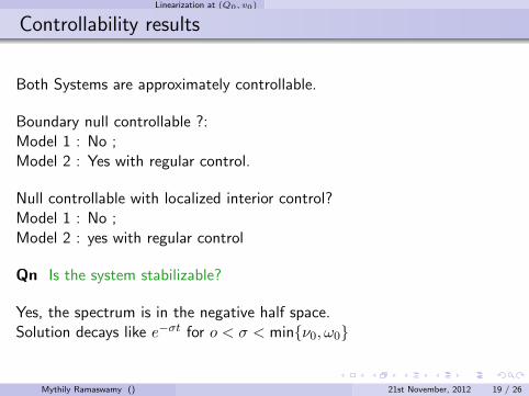
Both Systems are approximately controllable.
Boundary null controllable ?:Model 1 : No ;Model 2 : Yes with regular control.
Null controllable with localized interior control?Model 1 : No ;Model 2 : yes with regular control
Qn Is the system stabilizable?
Yes, the spectrum is in the negative half space.Solution decays like e−σt for o < σ < minν0, ω0
Mythily Ramaswamy () 21st November, 2012 19 / 26
Stabilizability
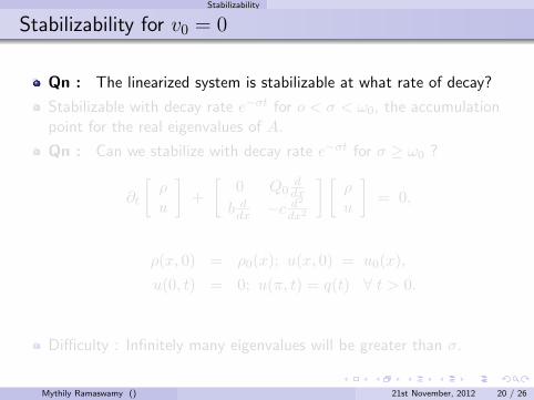
Stabilizability for v0 = 0
Qn : The linearized system is stabilizable at what rate of decay?
Stabilizable with decay rate e−σt for o < σ < ω0, the accumulationpoint for the real eigenvalues of A.
Qn : Can we stabilize with decay rate e−σt for σ ≥ ω0 ?
∂t
[ρu
]+[
0 Q0ddx
b ddx −c d2dx2
] [ρu
]= 0,
ρ(x, 0) = ρ0(x); u(x, 0) = u0(x),u(0, t) = 0; u(π, t) = q(t) ∀ t > 0.
Difficulty : Infinitely many eigenvalues will be greater than σ.
Mythily Ramaswamy () 21st November, 2012 20 / 26

Stabilizability
Projections of the system on eigenspaces
Outline of the method
Write the system as an operator equation
Project it onto one dimensional eigenspaces corresponding toeigenvalues accumulating at ω0
Find the expression for minimum norm control stabilizing this onedimensional projections
Find its limit as n tends to infinity
Mythily Ramaswamy () 21st November, 2012 21 / 26
Stabilizability
stabilizability
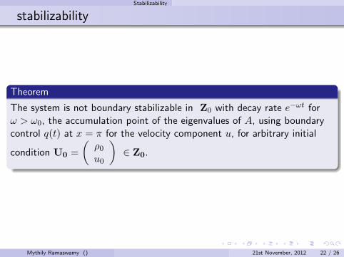
Theorem
The system is not boundary stabilizable in Z0 with decay rate e−ωt forω > ω0, the accumulation point of the eigenvalues of A, using boundarycontrol q(t) at x = π for the velocity component u, for arbitrary initial
condition U0 =(ρ0
u0
)∈ Z0.
Mythily Ramaswamy () 21st November, 2012 22 / 26
Extensions
System of equations including temperature
Equations for density, velocity and temperature
system of three equations for ρ, v, θ
Linearization around (Q0, 0, θ0)
Behaviour like parabolic system
Mythily Ramaswamy () 21st November, 2012 23 / 26

Extensions
Nonlinear system
Full nonlinear system near a stationary solution (ρ0, 0)
Can we stabilize the nonlinear system with the control found for thelinearized system?
Mythily Ramaswamy () 21st November, 2012 24 / 26

Extensions
Linearized system in a rectangle
Linearized system in 2 dimension in a rectangle
Fourier Basis for suitable boundary conditions
Null controllability for Dirichlet boundary conditions
Optimal control problem
Mythily Ramaswamy () 21st November, 2012 25 / 26

Extensions
Summary and Future work
Linearized Compressible Navier Stokes SystemCoupled system of transport and parabolic equations.
linearization at (Q0, 0) parabolic
linearization at (Q0, v0) hyperbolic
Questions
Computational aspects : Can we compute the control ?
Feedback control, observers?
Analysis of linearized system at nonconstant steady states?
Nonlinear system behaviour?
Other coupled systems?
Mythily Ramaswamy () 21st November, 2012 26 / 26
Extensions
S. Chowdhury and M. Ramaswamy, Optimal Control of LinearizedCompressible Navier-Stokes Equations, To appear in ESIAM : COCV -Control, Optimization and Calculus of Variations.
S. Chowdhury, M. Ramaswamy and J-P. Raymond, Controllability andstabilizability of the linearized compressible Navier-Stokes system inone dimension, To appear in SICON.
S. Chowdhury, D. Mitra, Controllability Results for LinearizedCompressible Navier Stokes System in One Dimension, Submitted
Mythily Ramaswamy () 21st November, 2012 26 / 26