Offi ce of Solid Waste andEmergency Response

January 2014www.epa.gov/superfund

Introduction toGroundwater Investigations

Superfund

United StatesEnvironmental ProtectionAgency

Workbook

TABLE OF CONTENTS

History of Colbert Landfill Page 1 Problem 1: Cross Section Exercise Page 3 Problem 2: Hydrogeological Exercise Page 15

Part 1: Determining Groundwater Flow Direction Page 15

Part 2: Groundwater Gradient and Seepage Velocity Calculation Page 20 Part 3: Falling Head Test Page 26

Problem 3: Performing an Aquifer Test Page 29 Problem 4: Groundwater Investigation Page 32 Glossary and Acronyms Page 45 Selected Hydrogeology Slides and Equations Page 53 Lecture Notes Page 65

HISTORY OF COLBERT LANDFILL, SPOKANE, WASHINGTON The Colbert Landfill is located 2.5 miles north of the town of Colbert near Spokane, Washington, and is owned by the Spokane County Utilities Department. This 40-acre landfill was operated from 1968 to 1986, when it was filled to capacity and closed. It received both municipal and commercial wastes from many sources. From 1975 to 1980, a local electronics manufacturing company disposed spent solvents containing methylene chloride (MC) and 1,1,1-trichloroethane (TCA) into the landfill. A local Air Force base also disposed of solvents containing acetone and methyl ethyl ketone (MEK). These solvents were trucked to the landfill in 55-gallon drums and poured down the sides of open and unlined trenches within the landfill. Approximately 300-400 gallons/month of MC and 150-200 gallons/month of TCA were disposed. In addition, an unknown volume of pesticides and tar refinery residues from other sources were dumped into these trenches.

The original site investigation was prompted by complaints from local residents who reported TCA contamination of their private wells. The population within 3 miles of the site is 1,500. In 1981, a Phase I investigation was conducted: a Phase 2 was completed in 1982. Groundwater samples collected from nearby private wells indicated TCA contamination at 5,600 µg/L, MC contamination at 2,500 µg/L, and acetone at a concentration of 445 µg/L. Investigation reports concluded that drinking groundwater posed the most significant risk to public health. EPA placed the site on the National Priority List (NPL) in 1983. Bottled water and a connection to the main municipal water system was supplied to residents with high TCA contamination (above the MCL), and the cost was underwritten by the potentially responsible parties (PRPs) involved.

Hydrogeological Investigation The site lies within the drainage basin on the Little Spokane River, and residents with private wells live on all sides of the landfill. The surficial cover and subsequent lower strata in the vicinity of the site consist of glacially derived sediments of gravel and sand, below which lie layers of clay, basaltic lava flows, and granitic bedrock. The stratigraphic sequence beneath the landfill from the top (youngest) to the bottom (oldest) is: Qa Alluvium or stream deposits composed of well-sorted and stratified silts, sands, and gravels Qfg Upper sand and gravel glacial outwash and Missoula flood deposits which together form a

water table aquifer Qglf Upper layers of glacial Lake Columbia deposits of impermeable silt and clay that serve as

an aquitard; lower layers of older glaciofluvial and alluvial sand and gravel deposits that form a confined aquifer

Mcl Impermeable and unweathered Latah Formation of silt and clay Kiat Fractured and unfractured granitic bedrock that serves as another confined aquifer

1

In the upper aquifer (Qfg), which is 8-15 feet thick, groundwater flows from 4 to 13 feet per day (ft/day). The lower confined sand and gravel aquifer (Qglf) varies from a few feet thick to 150 feet thick and is hydraulically connected to the Little Spokane River. Groundwater in this aquifer flows from 2 to 12 ft/day. To the northeast of the landfill, the upper aquifer is connected to the lower aquifer. Both of these aquifers are classified as current sources of drinking water according to EPA and are used locally for potable water. The area impacted by the site includes 6,800 acres and the contamination plume extends 5 miles toward the town of Colbert. Of the contaminants present, 90 percent occur as dense, nonaqueous-phase liquids (DNAPLs) at the bottom of the upper aquifer, and natural DNAPL degradation is slow. It has been estimated that only 10 percent of the solvents have gone into solution, whereas the remainder occurs in pore spaces and as pools of pure product above impermeable layers. The TCA plume in the upper aquifer has extended 9,000 feet in 8-10 years and it moves at a rate of 2-3 ft/day. The flow rate of the contamination plume in the lower sand and gravel aquifer (Qglf) has not been calculated because of the complexity and variability of the subsurface geology. However, TCA and MC have the highest concentrations in the lower sand and gravel aquifer.

2

PROBLEM 1: CROSS-SECTION EXERCISE

A. Student Performance Objectives

1. Draw a topographic profile of a specified area.

2. Calculate a vertical exaggeration for a topographic profile.

3. Obtain geological information from monitoring well logs.

4. Use the GSA Munsell color chart and McCulloch geotechnical gauge to identify rock sample colors and textures.

5. Given a geologic map, interpret surface elevations of geologic formations.

6. Draw a geologic cross section using monitoring well logs and a topographic

profile.

7. Interpret subsurface geology to locate aquifers of concern and identify discontinuities in geologic formations.

B. Background Information

Students will examine rock/sediment samples labeled A, B, C, E, or F. These samples represent rock/sediment samples from five different geologic formations encountered during the installation of monitoring wells at, and in the vicinity of, the Colbert Landfill site in Spokane, Washington. During the site investigation, these samples were collected from cuttings generated by Roto-Sonic drilling. Each sample is also oriented with an arrow that indicates the top.

C. Geologic Cross-Section

1. Using the GSA Munsell color chart and sample mask, match the overall color of the rocks, sand, clay, or gravel within the samples to the color chart. Do not determine every color if a sample is multicolored, but look for key sediment types or specific marker colors.

2. Using McCulloch’s geotechnical gauge, generally determine and match the grain size of the sediments with the written descriptions. For example, actual fine sand or coarse sand sizes can be found on the chart. Sediments larger than coarse sand, such as gravel and cobbles, are NOT shown on the geotechnical card. Using the geotechnical gauge and the sediment characteristics diagram depicted in Figure 1, generally determine the degree of particle rounding and sediment sorting. Well sorted means most particles are of similar size and shape, whereas poorly sorted particles are of no particular size and vary greatly in size and shape, such as sand mixed with gravel or cobbles.

3

3. Using the SAMPLES and well log together, match these descriptions and your visual observations to a geologic formation listed on the Description of Geologic Units for Cross-Section of Colbert Landfill. Then identify each formation on the well logs in the space provided under the “STRATA” column; for example, Kiat, sample F. START WITH WELL LOG #6, AND PROCEED TO LOG #1. EACH SAMPLE REPRESENTS ONLY A PORTION OF ONE ROCK FORMATION! Your instructor will discuss the correct sample identification at the end of this portion of the exercise.

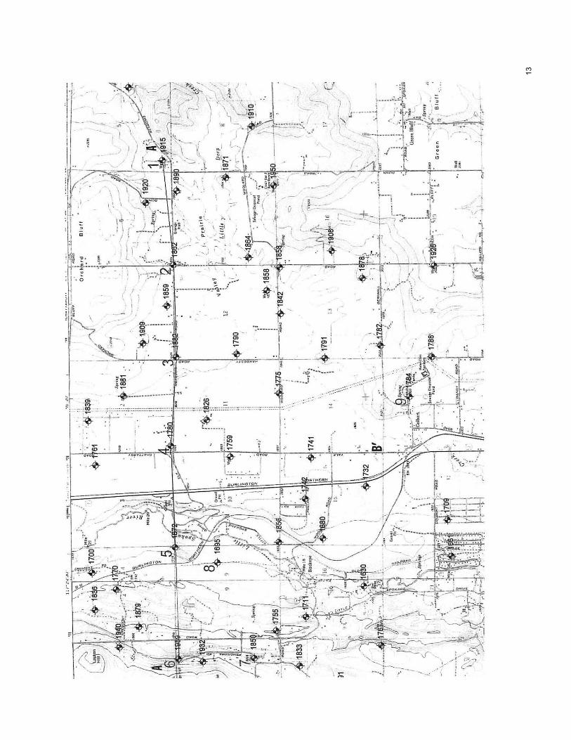
4. Using the appropriate topographic maps and graph paper provided, locate Wells 6

through 1 along the top of the graph paper from left to right along profile line A-A’. Determine the respective surface elevations of the wells (your instructor will demonstrate this technique).

5. Label the Y-axis of the graph paper to represent the elevation, starting from

2,100 feet at the top to 1,400 feet at the bottom. Each box on the graph represents 20 FEET in elevation.

6. Plot the location, depicting the correct surface elevation of each well on the

graph. Also determine and plot the elevations of SEVERAL EASILY DETERMINED POINTS on the profile line between each of the wells in order to add more detail to the profile. This will generate a series of dots representing the elevations of the six wells and the other elevations you have determined. Make sure to select contour lines that cross the profile line. The contour interval of this topographic map is 20 feet.

7. After plotting these elevations on the graph, connect them with a SMOOTH

CURVE, which will represent the shape of the topography from A-A’.

8. Using the well logs previously completed and the colored geologic map, add the existing geology and formation thickness to each well location. Each formation thickness must be determined by the depth on the left side of the well log.

9. Sketch in and interpret the geologic layers of the cross section, starting with the

lowest bedrock formation. Connect all of the same geologic formations, keeping in mind that some formations have varying thicknesses and areal extent.

10. Using available groundwater information shown on the well logs, locate the

shallow aquifer in the cross section.

11. Using the completed cross section, locate potential sites for the installation of additional monitoring wells or remediation wells and identify formation discontinuities.

12. Compare your interpretation with the “suggested” interpretation handed out by

the instructor.

4

`

5

DESCRIPTION OF GEOLOGIC UNITS IN THE AREA OF THE COLBERT LANDFILL – SPOKANE, WASHINGTON

MAP SYMBOL DESCRIPTION

Qa Alluvium or stream deposits (Holocene) – composed of silt, grayish-orange sand and gravel sediment that is well sorted and stratified. These deposits are found in flood plains, river terraces, and valley bottoms.

Qfg Flood deposits (Pleistocene) – poorly sorted, stratified mixture of boulders, gray cobbles, dark gray well-rounded gravel, and coarse sand resulting from multiple episodes of catastrophic outbursts from glacial-dammed lakes, such as glacial Lake Missoula. The Little Spokane River Valley was one of the main channelways for outburst flood waters from this ancient lake.

Qls Alluvial fan deposits (Pleistocene) – composed of unstratified and poorly sorted (heterogeneous and anisotropic) clay-, silt-, pink sand-, and gravel-size sediment. Some fan deposits contain large blocks of gray basaltic rock as much as 8 meters (26 feet) in diameter.

Qglf Lacustrine deposits (Pleistocene) – composed of crumbly sediment of white-clay, gray silt, and fine green sand, inter-bedded (mixed) with flood deposits (Pleistocene), composed of poorly sorted, but stratified mixtures of boulders, cobbles, gravel, and green sand.

Mvwp

COLUMBIA RIVER BASALT GROUP-TERTIARY (MIOCENE)

Wanapum extrusive basalt flows – composed of dense, greenish-black, and weathered basalt; some have a vesicular (mineral-filled gas bubble) texture.

Mcl Latah Formation – white to yellowish gray siltstone and claystone, grayish-green sandstone to lacustrine (lake) origin and grayish-orange sandstone from fluvial (river/stream) depositional environments.

INTRUSIVE IGNEOUS ROCK-CRETACEOUS PERIOD, MESOZOIC ERA

Kiat Mount Spokane granite – massive, medium-grained pale, reddish-brown granite that is present on Mount Spokane.

6

7

8

9

10

11

12

13

W 6

5

4

3

2

CO

LB

ER

T L

AN

DF

ILL

E

1"

= 8

0' V

ert

ical S

cale

1"

= 2

,000' M

ap S

cale

Pro

file

of

Colb

ert

Landfill,

Spokane,

Washin

gto

n

V.E

.= 2

5

V.E

.=1"/

80'

1"/

2000'

V.E

.=V

. S

ca

le

H. S

cale

14

PROBLEM 2: HYDROGEOLOGICAL EXERCISES PART 1. DETERMINING GROUNDWATER FLOW DIRECTION A. General Discussion

Methods for determining the direction of groundwater flow depend on the number of wells present on a particular site. When a site consists of only a few wells, a mathematical or graphical three-point problem can be used as shown in sections B and C. It is important to note that three-point problems can also be used to calculate the slope of the groundwater surface by dividing the difference in head (H1 - H3) by the measured map distance. When a site has a large number of wells, the slope of the groundwater surface can be calculated and depicted graphically by constructing a flow net, explained further in Part 2, section A.

B. The Mathematic Three-Point Problem for Groundwater Flow Groundwater-flow direction can be determined from water-level measurements made on

three wells at a site (Figure 1). 1. Given: Well Number Head (meters)

1 26.28 2 26.20 3 26.08

2. Procedure:

a. Select water-level elevations (head) for the three wells depicted in Figure 1. Label as H1, H2, and H3 in descending order.

b. Determine which well has a water-level elevation between the other wells (Well 2). c. Draw a line between Wells 1 and 3. Note that somewhere between these

wells is a point, labeled A in Figure 2, where the water-level elevation at this point is equal to Well 2 (26.20 m).

d. To determine the distance X from Well 1 to point A, solve the following equation (see Figure 3, 4, and 5):

H1 – H3 H1 – H2

Y = X e. Distance Y is measured directly from the map

(200 m) on Figure 3. f. After distance X is calculated, groundwater-flow direction based on the

water-level elevations can be constructed 90° to the line representing equipotential elevation of 26.20 m (Figure 6).

15

16

17

18

C. The Graphical Three-Point Problem for Groundwater Flow

Groundwater-level data can be used to determine direction of groundwater flow by constructing groundwater contour maps and flow nets. To calculate a flow direction, at least three observation points are needed. First, relate the groundwater field levels to a common datum – map datum is usually best – and then accurately plot their position on a scale plan. Second, draw a pencil line between each of the observation points, and divide each line into a number of short, equal lengths in proportion to the difference in elevation at each end of the line (Figure 7). The third step is to join points of equal height on each of the lines to form contour lines (lines of equal head). Select a contour interval that is appropriate to the overall variation in water levels in the study area. The direction of groundwater flow is at right angles to the contour lines from points of higher head to points of lower head (Figure 8).

19

PART 2. GROUNDWATER GRADIENT and SEEPAGE VELOCITY CALCULATION

A. Purpose

This part of the exercise uses basic principles defined in the determination of groundwater-flow directions. Groundwater gradients (slope of the top of the groundwater table) will be calculated as shown in the three-point problem. The three point procedure can be applied to a much larger number of water-level values to construct a groundwater-level contour map. Locate the position of each observation point on a base map of suitable scale and write the water level next to each well’s position. Study these water-level values to decide which contour lines would cross the center of the map. Select one or two key contours to draw in first. Once the contour map is complete, flow lines can be drawn by first dividing a selected contour line into equal lengths. Flow lines are drawn at right angles from this contour, at each point marked on it. The flow lines are extended until the next contour line is intercepted, and are then continued at right angles tot his new contour line. Always select a contour that will enable you to draw the flow lines in a downgradient direction.

B. Key Terms

Head – The energy contained in water mass produced by elevation, pressure, and/or velocity. It is a measure of the hydraulic potential due to pressure of the water column above the point of measurement and height of the measurement point above datum which is generally mean seal level. Head is usually expressed in feet or meters.

Contour line – A line that represents the points of equal values (e.g.,

elevation, concentration).

Equipotential line – A line that represents the points of equal head of groundwater in an aquifer.

Flow lines – Lines indicating the flow direction followed by groundwater

toward points of discharge. Flow lines are always perpendicular to equipotential lines. They also indicate direction of maximum potential gradient.

20

21

22

23

Calculation of Seepage Velocity (Vs) Vs = KI Ne Given a hydraulic conductivity (K) of 5 ft/day and an effective porosity (Ne) of 15%; solve the amount of time (in Days) for groundwater to travel from point A to point B.

Vs = KI Ne Vs = (5 ft/day) (0.017 ft/ft) 0.15 Vs = 0.56 ft/day

Given a distance between Point A to B = 600 feet and using the velocity equation of (Vs) (Time) = Distance Time = Distance Vs Time = 600 ft = 1071 Days or 2.9 Years 0.56 ft/day

24

Vs Time = 600 ft = 1071 Days or 2.9 Years 0.56 ft/day

Key

Vs = Seepage velocity K = Hydraulic conductivity I = Gradient Ne = Effective porosity

C. Groundwater Gradient, Colbert Landfill

Overlay the transparent sheet on top of the Colbert Landfill topographic map. Tape down to hold in place, and mark a few reference points to ensure correct placement throughout the exercise (i.e., make a “+” on an intersection or reference line on the map). Select an appropriate contour interval that fits the water levels available and the size of the map. Fifty-foot contour intervals should be appropriate for this problem. Draw the equipotential lines on the map interpolating between water-level measurements. Paragraph two of the Purpose also explains this technique. Construction flow lines perpendicular to the equipotential lines drawn in step 4 and discussed in paragraph three of Purpose.

25

PART 3. Falling Head Test Exercise A. Student Performance Objectives

1. Perform a falling head test on geologic materials.

2. Calculate total porosity, effective porosity, and estimated hydraulic conductivity. B. Perform a Falling Head Test

1. Set up burets using the stands and tube clamps.

2. Clamp the rubber tube at the bottom of the burets using the hose clamp. Fold the rubber hose to ensure a good seal before clamping (to help eliminate leaking water).

3. Position the small, round screen pieces in the bottom of the burets. Use the tamper

to properly position the screens.

4. Measure 250 ml of colored water in the 500 ml plastic beaker.

5. Pour the water slowly into the buret to avoid disturbing the seated screen.

6. Measure 500 ml of gravel or sand material in the 500 ml plastic beaker.

7. Pour the gravel or sand slowly into the water column in the buret to prevent the disturbance of the screen traps and to allow any trapped air to flow to the surface of the water in the buret.

8. Add additional measured quantities of water or gravel/sand as needed until both

the water and sediment reach the zero mark on the buret. To calculate the final total volumes of water and sediment, add the volumes of additional water and gravel/sand to the initial volumes of 250 and 500 ml of water and sediment. The total volumes of water and sediment are designated W and S respectively.

9. Measure the static water level in the buret to the base of the buret stand. This is

the total head of the column of water at this elevation. This measurement is designated h0.

10. Place a plastic, 500 ml graduated beaker below the buret. (The beaker will be used

to collect the water drained from the buret.) The volume of water in the beaker is designated WD.

11. Undo the clamp and simultaneously start the timer to determine the flow rate of

water through the buret. When the drained water front reaches the screen, stop the timer, clamp the buret hose, and record the elapsed time. Also record the volume of water drained during this time interval. This time is designated t.

26

12. Allow the water level in the buret to stabilize. Measure the length from this

level to the base of the buret stand. This is the total head of the water column at this elevation after drainage has occurred. This measurement is designated h1.

13. Subtract the measurement at h1 from the height measurement at h0. This length

is designated L.

14. The porosity in the sediment of each buret is the volume of water necessary to fill the column of sediment in the buret to the initial static water mark at h0

divided by the sediment volume (S). This value is total porosity and is designated N.

15. The effective porosity is estimated by dividing the volume of drained water by

the sediment volume. Effective porosity is designated n.

16. Compare the initial volume of water (W) in the column before draining with the drained volume (WD). The difference represents the volume of water retained (WR), or the specific retention. The volume drained represents specific yield. To determine the percent effective porosity, divide the volume of drained water by the volume of total sediment volume.

17. The equation to estimate the hydraulic conductivity (K) of each buret column

is derived from falling head permeameter experiments. The equations for this exercise are depicted below.

27

TABLE 2. TOTAL HEAD WORKSHEET

Sample Number

Volume Sediment (S)

Volume Water (W)

Volume Drained Water (WD)

Volume Retained Water

Total Porosity Calculated (N)

Effective Porosity Calc. (n)

Length (h0 –h1)

Time (t)

Initial Head (H0)

Final Head (H1)

ln (h0/h1)

Est. Hydraulic Conductivity (K)

Total Porosity Effective Porosity Est. Hydraulic Cond. N = W n = WD K = [2.3 x L] x ln (h0/h1) S S [ t ]

28

PROBLEM 3: PERFORMING AN AQUIFER TEST JACOB TIME-DRAWNDOWN METHOD

A. Background Information

Each student will be given a sheet of semilogarithmic graph paper. Then, they should follow these directions:

1. Orient the semi-log paper, so the three-hole punches are at the top of the page. Label the long horizontal logarithmic axis (the side with the punched holes) of the graph paper t-times (minutes). Leave the first numbers (1 through 9) as is. Mark the next series of heavy lines from 10 to 100 in increments of 10 (10, 20, 30, etc.). Mark the next series from 100 to 1000 in increments of 100 (100, 200, 300, etc.).

2. Label the short vertical arithmetic axis s-drawdown (feet). This will be

the drawdown (s) measured from the top of the casing (provided in Table 1). mark off the heavy lines by tens, starting with 0 at the top, then 10, 20, 30, 40 50, 60 and 70 (the bottom line). Each individual mark represents 1 foot.

3. Plot the data in Table 1 on the semilogarithmic paper with the values

for drawdown on the arithmetic scale and corresponding pumping times on the logarithmic scale.

4. Draw a best-fit straight line through the data points. 5. Compute the change in drawdown over one log cycle where the data

plot as a straight line. 6. Using the information given in Table 1 (Q = 109 gpm and b = 20 feet)

and Jacob’s formula shown below, calculate the value for hydraulic conductivity.

ΔS = ft T = 35Q T = ft2/day ΔS K = T K = ft/day b

29

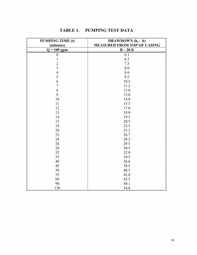
TABLE 1. PUMPING TEST DATA

PUMPING TIME (t)

(minutes) DRAWDOWN (ho – h)

MEASURED FROM TOP OF CASING Q = 109 gpm B – 20 ft

0 6.1 1 6.5 2 7.5 3 8.0 4 8.6 5 9.5 6 10.5 7 11.2 8 12.0 9 13.0 10 14.0 11 15.5 12 17.0 13 18.0 14 19.3 15 20.5 18 23.5 20 25.2 22 26.7 24 28.2 26 29.5 28 30.5 32 32.0 35 34.5 40 36.6 45 38.5 50 40.5 55 42.0 60 43.5 90 50.1 120 54.8

30

PROBLEM 3: PERFORMING AN AQUIFER TEST

HVORSLEV SLUG TEST

A slug test is performed by lowering a metal slug into a piezometer that is screened in a silty clay aquifer. The inside diameter of both the well screen and the well casing is 2 inches. The borehole diameter is 4 inches. The well screen is 10 feet in length. The following data were obtained when the slug was rapidly pulled from the piezometer:

TABLE 2. SLUG TEST DATA

ELAPSED TIME (minutes)

DEPTH TO WATER (feet)

CHANGE IN WATER LEVEL h (feet)

h/ho

Static level 13.99 0 14.87 0.88 (ho) 1.000 1 14.59 0.60 0.682 2 14.37 0.38 0.432 3 14.20 0.21 0.239 3 14.11 0.12 0.136 5 14.05 0.06 0.068 6 14.03 0.04 0.045 7 14.01 0.02 0.023 8 14.00 0.01 0.011 9 13.99 0.00 0.000

The time for the head to rise or fall to 37 percent of the initial value is To. The following values are obtained from the geometry of the piezometer:

r = 0.083 feet R = 0.166 feet L = 10.0 feet

1 cm/sec = 2835 ft/day

The ratio L/R is 60.24, which is more than 8, so the following equation is used:

r2ln(L/R) 2LTo

K =

31

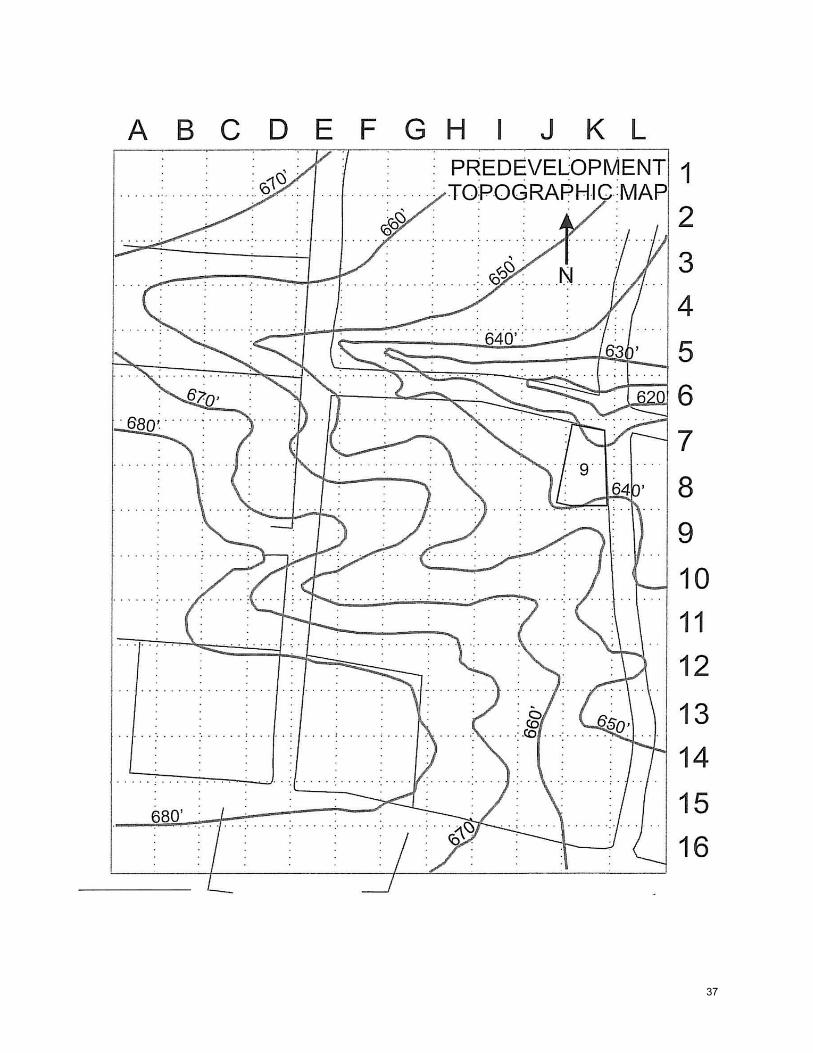
PROBLEM 4. GROUNDWATER INVESTIGTION BETTENDORF, IOWA

A. Student Performance Objectives

1. This will be your final examination. Based on your performance, you and your group will be evaluated on your findings and conclusions that you presented to your peers.

2. Perform a site investigation using soil gas surveys and monitoring wells. 3. Determine the source(s) of hydrocarbon contamination at a contaminated site. 4. Present the results of the field investigation to the class. 5. Justify the conclusions of the field investigation.

B. Desktop and Other Background Information History of the Leavings’ Residence

On October 12, 1982, the Bettendorf, Iowa, fire department was called to the Leavings’ residence with complaints of gasoline vapors in the basement of the home. On October 16, 1982, the Leavings were required to evacuate their home for an indefinite period of time until the residence could be made safe for habitation. The gasoline vapors were very strong, so electrical service to the home was turned off. Basement windows were opened to reduce the explosion potential.

32

Pertinent Known Facts

The contaminated site is in a residential neighborhood in Bettendorf, Iowa. It borders on commercially zoned property, which has only been partially developed to date. The residential area is about 10 years old and contains homes in the $40,000 to $70,000 range. There was apparently some cutting and filling activity at the time the area was developed. Within ¼ mile to the northwest and southwest, 11 reported underground storage tanks (USTs) are in use or have only recently been abandoned:

* Two tanks owned and operated by the Iowa Department of Transportation (IDOT) are located 1000 ft northwest of the site.

* Three in-place tanks initially owned by Continental Oil, and now by U-Haul,

are located 700 ft southwest of the site. According to the Bettendorf Fire Department (BFD), one of the three tanks reportedly leaked.

* Three tanks owned and operated by an Amoco service station are located 1200

ft southwest of the site. BFD reports no leaks. * Three tanks owned and operated by a Mobil Oil service station are located 1200

ft southwest of the site. BFD reports no leaks.

Neighbors that own lots 8 and 10, which adjoin the Leavings residence (Lot 9), have complained about several trees dying at the back of their property. No previous occurrences of gasoline vapors have been reported at these locations. The general geologic setting is Wisconsin loess sediments mantling Kansan and Nebraskan glacial till. Valleys may expose the till surface on the side slope. Valley sediment typically consists of alluvial silts. Previous experience by your environmental consulting firm in this area includes a geotechnical investigation of the hotel complex located west of Utica Ridge Road and northwest of the Amoco service station. Loess sediments ranged from 22 ft thick on the higher elevations of the property (western half) to 10 ft thick on the side slope. Some silt fill (5-7 ft) was noted at the east end of the hotel property. Loess was underlain by a gray, clayey glacial till which apparently had groundwater perched on it. Groundwater was typically within 10-15 ft of ground surface. This investigation was performed 8 years ago and nothing in the boring logs indicated the observation of hydrocarbon vapors. However, this type of observation was not routinely reported at that time. Other projects in the area included a maintenance yard pavement design and construction phase testing project at the IDOT facility located northwest of the Leavings residence. Loess sediments were also encountered in the shallow pavement subgrade project completed 3 years ago. Consulting firm records indicated that the facility manager reported a minor gasoline spill a year before and that the spill had been cleaned up when the leaking tank was removed and replaced with a new steel tank. The second tank at the IDOT facility apparently was not replaced at that time.

33

Results of Site Interviews

Lot 9 (THE Leavings’ residence): Observations outside the residence indicate that the trees are in relatively good condition. The house was vacant. Six inches of free product that looks and smells like gasoline was observed in the open sump pit in the basement. The power to the residence was turned off, so the water level in the sump was allowed to rise. The fluid level in the sump was about 3 feet below the level of the basement floor.

Neighbors (Lots 8 and 10): These property owners reported that several trees in

their backyards died during the past spring. They contacted the developer of the area (who also owns the commercial property that adjoins their lots) and complained that the fill that was placed there several years ago killed some of their trees. No action was taken by the developer. Both neighbors said that when the source of the as was located, they wanted to be notified so they could file their own lawsuits. The neighbors also noted that this past September and October were unusually wet (lots of rainfall).

IDOT: The manager remembers employees from your firm testing his parking lot.

He reported that one UST was replaced in 1979, whereas the other tank was installed when the facility was built in 1967. Both of the original tanks were bare metal tanks. The older replaced tank always contained gasoline, but the newer one contains diesel fuel. No inventory records or leak testing records are available. The manager stated that he has never had any water in his tanks. He will check with his supervisor to have the USTs precision leak tested.

U-Haul: The manager said that the station used to be a Continental Oil station with

three USTs. The three USTs were installed by Continental in 1970 when the station was built. Currently, only one 6000-gal UST (unleaded) remains in service for the U-Haul fleet. This tank was found to be leaking a month ago, but the manager does not know how much fuel leaked.

Mobil: The manager was pleasant until he found out the purpose of the interview.

He did state that he built the station in 1970 and installed three USTs at that time. He would not answer any additional questions.

Amoco: The manager was not in, but an assistant provided his telephone number. In

a telephone interview, the manager said he was aware of the leaking tank at the U-Haul factory and was anxious to prove the product was not from his station. He said they installed three USTs for unleaded, premium, and regular gasoline in 1972. An additional diesel UST was installed in 1978. The tanks are tested every 2 years using the Petrotite test method. The tanks have always tested tight. No inventory control system is being used at present. He stated that if monitoring wells were needed on his property, he would be happy to cooperate.

34

Developer (Mr. M. Forester): Mr. Forester bought the property in question in the 1960s. He developed the residential area first and some of the commercial development followed. About 40 acres remain undeveloped to date. He plans to build a shopping center on the remaining 40 acres in the future.

Mr. Forester obtained a lot of cheap dirt and fill when the interstate cut went through about ½ mile west of the property in the late 1960s. He filled in a couple of good-sized valleys at that time. He has a topographic map of the area after it was filled. He stated that he will cooperate fully with any investigation. If any wells are needed on the property, he would like to be notified in advance. There are no buried utilities on the property except behind the residential neighborhood.

Review of Bettendorf City Hall Records An existing topographic map and scaled land use map are included in this exercise. Ownership records indicate the land was previously owned by Mr. and Mrs. Ralph Luckless. The city hall clerk stated that she had known them prior to the sale of the farm in 1964. Zoning at that time was agricultural only. The section of the farm now in question was primarily used for grazing cattle because it was too steep for crops. The clerk remembered a couple of wooded valleys in that same field. She also remembered a muddy stream that used to run where Golden Valley Drive is now and that children used to swim in it. She also stated that one valley was between Golden Valley Drive and where all the fill is now (near U-Hal and Amoco). The current owner of the underdeveloped property is Mr. M. Forester, a developer with an Iowa City, Iowa address. There is no record of storm of sanitary sewer lines along Utica Ridge Road south of Golden Valley Drive. Storm and sanitary sewer lines run along Spruce Hills Drive.

Iowa Ecological Survey Information There are no records of any wells in the section. In an adjoining section, wells indicate top of bedrock at about 650 feet mean sea level (MSL). The uppermost usable aquifer is the Mississippian-age limestone for elevations from 350 feet to 570 feet MSL. The materials overlying the Mississippian are Pennsylvanian shales and limestone. Soil Conservation Survey Maps The 1974 edition indicates “Made Land” over nearly all of the area not designated as commercial zone. Made Land normally indicates areas of cut or fill.

35

36

37

38

ASSIGNMENT: FIELD INVESTIGATION

TABULATION OF FEES FOR FIELD INVESTIGATION GROUP__________

WORKSHEET #1 # UNITS COST TOTAL

Recommendations for making residence habitable 1 each $500 LS

(lump sum) $

Soil gas survey – mobilization fee 1 each $500 LS $

Soil gas survey $1500/ac

Monitoring wells – mobilization fee 1 each $500 LS $

2” PVC 15 ft screen – 25 ft deep

$1200 ea

2” stainless steel 15 ft screen – 25 ft deep

$1700 ea $

Well security – locking protector pipe $300 ea $

Field investigation engineering analysis and report

1 each 15%

$2000 min $

TOTAL COST

$

SITE INVESTIGATION FIELD ACTIVITIES

AT BETTENDORF, IOWA

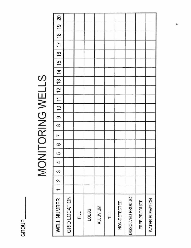
Each team is to perform a site investigation. (The instructors will select the groups.) All public written information has been provided, and we expect your team to gather field data and other information from us in order to identify the responsible parties for the contamination at the Leavings’ residence. Your group will need to select where to install monitoring wells and conduct soil gas surveys. Use the table on page 10 for monitoring well data and the base map on page 11 for soil gas survey results. The following caveats are a guide of activities for your group to follow while completing this task. 1. Teams will be determined by the instructors. 2. Review all prior desktop information. 3. Organize your effort in gathering more data and information. a. Determine the location of the groundwater table by installing monitoring wells. b. Determine source(s) of contamination and define the shape of the contaminant plume(s) on top of the groundwater table using i. Data from monitoring wells ii. Soil gas survey results c. Construct a cross section normal to groundwater flow. d. Determine hydraulic conductivity using slug test data. e. Calculate transport time of contaminants. f. Calculate cost of investigation.

39

40

41

Scale: | | = 100 ft

42

Group #:________

FINAL GROUNDWATER PROBLEM: BETTENDORF, IOWA

Each group of students will determine, identify, draw, and calculate the items below and include them in brief class presentation. Group scores (out of 100%) are based upon completion of each category below. SCORE: __________ 1. Determine groundwater flow direction by constructing a groundwater surface contour map and a flow net (not a 3-point problem) on the site map provided. __________ 2. Identify the source(s) that contributed to the Leavings’ groundwater problem. __________ 3. Sketch a contaminant plume map from your collected subsurface date on the site

map sheet provided. __________ 4. Draw a geologic cross section that lies perpendicular to the direction of the

groundwater flow; identify geologic units and groundwater level on the graph paper provided.

__________ 5. Using your groundwater surface contour map, calculate the hydraulic gradient (I)

in feet per foot between the source and the Leavings’ residence. __________ 6. Plot your slug test data on the semi-log sheet provided. Label your axes. __________ 7. Calculate the hydraulic conductivity (K) value in feet per day using the Hvorsley

Method and the slug test data provided. Show calculations on the graph paper. __________ 8. Calculate the seepage velocity (v) in feet per day using vs = KL/ne with an effective

porosity (ne) value of 0.05. __________ 9. Calculate an approximate transport time in years of the contaminant from the

source to the Leavings’ residence using the equation: vsT (time in years) = D (distance in feet).

__________ 10. Determine your final cost for conducting this hydrogeologic investigation:

$___________. __________ TOTAL GROUP SCORE: (To be filled in by Course Director.)

Print group member names below:

a. e.

b. f.

c. g.

d. h.

43

LEAVINGS’ RESIDENCE SITE, IOWA SLUG TEST RESULTS

MW-6, Grid Location at E-12

44

Introduction to Groundwater Investigations

GLOSSARY AND ACRONYMS

acre-foot enough water to cover 1 acre to a depth of 1 foot; equal to 43,560 cubic feet or 325,851 gallons adsorption the attraction and adhesion of a layer of ions from an aqueous solution to the solid mineral surfaces with which it is in contact advection the process by which solutes is transported by the bulk motion

of the flowing groundwater alluvium a general term for clay, silt, sand, gravel, or similar unconsolidated material deposited during comparatively

recent geologic time by a stream or other body of running water as sorted or semisorted sediment in the bed of the stream or on its floodplain or delta, or as a cone or fan at the base of a mountain slope

anisotropic hydraulic conductivity (“K”), differing with direction aquifer a geologic formation, group of formations, or a part of a

formation that contains sufficient permeable material to yield significant quantities of groundwater to wells and springs. Use of the term should be restricted to classifying water bodies in accordance with stratigraphy or rock types. In describing hydraulic characteristics such as transmissivity and storage coefficient, be careful to refer those parameters to the saturated part of the aquifer only.

aquifer test a test involving the withdrawal of measured quantities of water

from, or the addition of water to, a well (or wells) and the measurement of resulting changes in head (water level) in the aquifer both during and after the period of discharge or addition

aquitard a saturated, but poorly permeable bed, formation, or group of

formations that does not yield water freely to a well or spring artesian confined; under pressure sufficient to raise the water level in a

well above the top of the aquifer artesian aquifer see confined aquifer artificial recharge recharge at a rate greater than natural, resulting from

deliberate or incidental actions of man

45

Introduction to Groundwater Investigations

BTEX benzene, toluene, ethylbenzene, and xylenes capillary zone negative pressure zone just above the water table where

water is drawn up from saturated zone into matrix pores due to cohesion of water molecules and adhesion of these molecules to matrix particles. Zone thickness may be several inches to several feet depending on porosity and pore size.

capture the decrease in water discharge naturally from a ground-water reservoir plus any increase in water recharged to the reservoir

resulting from pumping coefficient of storage the volume of water an aquifer releases from or takes into storage per unit surface area of the aquifer per unit change in head cone of depression depression of heads surrounding a well caused by withdrawal

of water (larger cone for confined aquifer than for unconfined) confined aquifer geological formation capable of storing and transmitting water in usable quantities overlain by a less permeable or impermeable formation (confining layer) placing the aquifer under pressure confining bed a body of “impermeable” material stratigraphically adjacent to one or more aquifers diffusion the process whereby particles of liquids, gases, or solids intermingle as a result of their spontaneous movement caused by thermal agitation discharge velocity an apparent velocity, calculated from Darcy’s law, which

represents the flow rate at which water would move through the aquifer if it were an open conduit (also called specific discharge)

discharge area an area in which subsurface water, including both groundwater and water in the unsaturated zone, is discharged to the land surface, to surface water, or to the atmosphere

dispersion the spreading and mixing of chemical constituents in

groundwater caused by diffusion and by mixing due to microscopic variations in velocities within and between pores

46

Introduction to Groundwater Investigations

DNAPL dense, non-aqueous phase liquid drawdown the vertical distance through which the water level in a well is

lowered by pumping from the well or nearby well effective porosity the amount of interconnected pore space through which fluids

can pass, expressed as a percent of bulk volume. Part of the total porosity will be occupied by static fluid being held to the mineral surface by surface tension, so effective porosity will be less than total porosity.

evapotranspiration the combined loss of water from direct evaporation and

through the use of water by vegetation (transpiration) flow line the path that a particle of water follows in its movement

through saturated, permeable materials gaining stream a steam or reach of a stream whose flow is being increased by

inflow of groundwater (also called an effluent stream) gpm gallons per minute groundwater reservoir all rocks in the zone of saturation (see also aquifer) groundwater divide a ridge in the water table or other potentiometric surface from which groundwater moves away in both directions normal to

the ridge line groundwater system a groundwater reservoir and its contained water; includes

hydraulic and geochemical features groundwater model simulated representation of a groundwater system to aid

definition of behavior and decision-making groundwater water in the zone of saturation head combination of elevation above datum and pressure energy

imparted to a column of water (velocity energy is ignored because of low velocities of groundwater). Measured in length units (i.e., feet or meters).

heterogeneous geological characteristics varying aerially or vertically in a

given system homogeneous geology of the aquifer is consistent; not changing with

direction or depth

47

Introduction to Groundwater Investigations

hydraulic conductivity volume flow through a unit cross-section area per unit decline

in head hydraulic gradient change of head values over a distance H1 – H2 L where: H = head L = distance between head measurement points hydrogeology the study of interactions of geologic materials and processes

with water, especially groundwater hydrograph graph that shows some property of groundwater or surface

water as a function of time impermeable having a texture that does not permit water to move through it

perceptibly under the head difference that commonly occurs in nature

infiltration the flow of movement of water through the land surface into

the ground interface in hydrology, the contact zone between two different fluids intrinsic permeability pertaining to the relative ease with which a porous medium

can transmit a liquid under a hydrostatic or potential gradient. It is a property of the porous medium and is independent of the nature of the liquid or the potential field.

isotropic hydraulic conductivity (“K”) is the same regardless of direction K hydraulic conductivity (measured in velocity units and

dependent on formation characteristics and fluid characteristics)

laminar flow low velocity flow with no mixing (i.e., no turbulence) LNAPL light, non-aqueous phase liquid losing stream a stream or reach of a stream that is losing water to the

subsurface (also called an influent stream)

48

Introduction to Groundwater Investigations

mining in reference to groundwater, withdrawals in excess of natural replenishment and capture. Commonly applied to heavily pumped areas in semiarid and arid regions, where opportunity for natural replenishment and capture is small. The term is hydrologic and excludes any connotation of unsatisfactory water-management practice

MSL mean sea level non-steady state (also called non-steady shape or unsteady shape) the

condition when non-steady shape the rate of flow through the aquifer is changing and water levels are declining. It exists during the early stage of withdrawal when the water level throughout the cone of depression is declining and the shape of the cone is changing at a relatively rapid rate.

steady state (also called steady shape) is the condition that exists during

the intermediate stage of withdrawals when the water level is still declining but the shape of the central part of the cone is essentially constant

optimum yield the best use of groundwater that can be made under the

circumstances; a use dependent not only on hydrologic factors but also on legal, social, and economic factors

overdraft withdrawals of groundwater at rates perceived to be excessive

and, therefore, an unsatisfactory water-management practice (see also mining)

perched aquifer a zone of saturation in a formation that is discontinuous from

the water table and the unsaturated zones surrounding this formation. Some regulatory agencies include an upper limit on the hydraulic conductivity of the perched aquifer

permeability the property of the aquifer allowing for transmission of fluid

through pores (i.e., connection of pores) permeameter a laboratory device used to measure the intrinsic permeability

and hydraulic conductivity of a soil or rock sample piezometer a non-pumping well, generally of small diameter, that is used

to measure the elevation of the water table or potentiometric surface. A piezometer generally has a short well screen through which water can enter.

49

Introduction to Groundwater Investigations

porosity the ratio of the volume of the interstices or voids in a rock or soil to the total volume

potentiometric surface imaginary saturated surface (potential head of confined

aquifer); a surface that represents the static head; the levels to which water will rise in tightly cased wells

recharge the processes of addition of water to the zone of saturation recharge area an area in which water that enters the subsurface eventually

reaches the zone of saturation safe yield magnitude of yield that can be relied upon over a long period

of time (similar to sustained yield) saturated zone zone in which all voids are filled with water (the water table is

the proper limit) slug-test an aquifer test made by either pouring a small instantaneous

charge of water into a well or by withdrawing a slug of water from the well (when a slug of water is removed from the well, it is also called a bail-down test)

specific yield ratio of volume of water released under gravity to total volume

of saturated rock specific capacity the rate of discharge from a well divided by the drawdown in it.

The rate varies slowly with the duration of pumping, which should be stated when known.

steady-state the condition when the rate of flow is steady and water levels

have ceased to decline. It exists in the final stage of withdrawals when neither the water level nor the shape of the cone is changing.

storage coefficient “S” volume of water taken into or released from aquifer storage

per unit surface area per unit change in head (dimensionless) (for confined, S = 0.0001 to 0.001; for unconfined, equal to porosity)

storage in groundwater hydrology, refers to 1) water naturally detained

in a groundwater reservoir, 2) artificial impoundment of water in groundwater reservoirs, and 3) the water so impounded

50

Introduction to Groundwater Investigations

storativity the volume of water an aquifer releases from or takes into storage per unit surface area of the aquifer per unit change in head (also called coefficient of storage)

sustained yield continuous long-term groundwater production without

progressive storage depletion (see also safe yield) transmissivity the rate at which water is transmitted through a unit width of

an aquifer under a unit hydraulic gradient unsaturated zone the zone containing water under pressure less than that of the (vadose zone) atmosphere, including soil water, intermediate unsaturated

(vadose) water, and capillary water. Some references include the capillary water in the saturated zone. This upper limit of this zone is the land surface and the lower limit is the surface of the zone of saturation (i.e., the water table).

water table surface of saturated zone area at atmospheric pressure; that

surface in an unconfined water body at which the pressure is atmospheric. Defined by the levels at which water stands in wells that penetrate the water body just far enough to hold standing water.

51

52

Selected hydrogeology slides 

and equations

Stream Flow

Q = Av

A (cross‐sectional area)

Q (discharge)

v (velocity)

POROSITY(Nt)

The volumetric ratio between the void spaces (Vv) and total rock (Vt):

Nt = Vv

Vt

;   Nt = Sy + Sr

Sy = specific yield

Sr = specific retention

53

Porosity

TOTAL POROSITY (Nt):

CLAY

SAND

GRAVEL

EFFECTIVE  POROSITY (Ne):

40‐85%

25‐50%

25‐45%

1‐10%

10‐30%

15‐30%

Total Head(ht)

• Combination of elevation (z) and pressure head (hp)

• Total head is the energy imparted to a column of water

ht = z + hp

GROUNDWATER LEVEL

PRESSUREHEAD

HYDRAULIC

OR

TOTALHEAD

ELEVATIONHEAD

DATUM(usually sea level)

POINT OFMEASUREMENT

(hp)

(ht)

(z)

54

Unconfined Aquifer

VADOSEZONE

CONFINING UNIT ‐AQUITARD

WATERTABLE

VERTICAL EQUIPOTENTIAL LINES

GROUNDWATERFLOW

UNCONFINED AQUIFER

GROUNDWATERFLOW

100 90 70 60 50 40

Confined Aquifer

CONFINED AQUIFER

CONFINING UNIT ‐AQUITARD

POTENTIOMETRICSURFACE

CONFINING UNIT 

AQUITARD

BASE OF UPPER CONFINING UNIT

VADOSEZONE

WATER TABLE

VADOSEZONERECHARGE

CONFINING LAYERS(AQUITARDS)

55

Artesian Groundwater System

AQUITARDS

POTENTIOMETRIC SURFACE

RECHARGE AREARECHARGE AREA

AQUIFER

AQUITARDS

POTENTIOMETRIC SURFACE

FLOWINGARTESIAN WELL

OVERBURDENPRESSURE

HYDRAULICPRESSURE

GWFLOW

Artesian Groundwater System

• Q = discharge• K = hydraulic  

conductivity• I  = hydraulic gradient• A = area

Darcy's LawQ = KIA

( ) dhdl

56

• The flow rate through a porous material is proportional to the head loss and inversely proportional to the length of the flow path

• Valid for laminar flow

• Assume homogeneous and isotropic conditions

Darcy's Law

Hydraulic Conductivity(K)

The volume of flow through a unit 

cross section of an aquifer per unit 

decline of head.

Q

dh

dl

HYDRAULICCONDUCTIVITY

AQUITARD

CONFINEDAQUIFER

AQUITARD

57

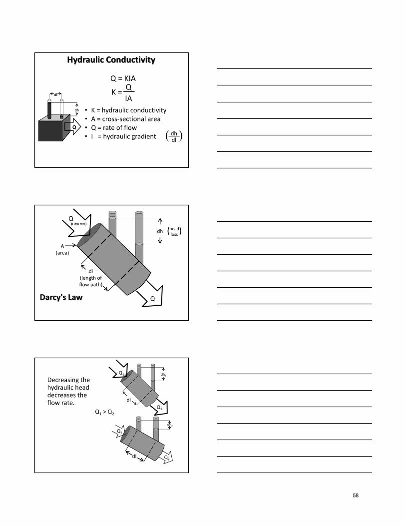
• K = hydraulic conductivity• A = cross‐sectional area• Q = rate of flow• I   = hydraulic gradient

Hydraulic Conductivity

QQ = KIA

IAK = 

( ) dhdl

Q

dh

dl

(    )

Q

Q(Flow rate)

dh

dl(length offlow path)

A(area)

headloss

Darcy's Law 

Decreasing the hydraulic head decreases the flow rate. dl

dh1

dl

dh2

Q1 > Q2

Q1

Q1

Q2

Q2

58

dh

dl1

dl2

Increasing the flow path length decreases the flow rate. Q1 > Q2

dh

Q1

Q1

Q2

Q2

• Darcy's Law     Q = KIA or         = Kl       QA

Groundwater Velocity

• Velocity equation     Q = Av  or         = v       

• v = KI   Darcian velocity      

By combining, obtain:

QA

• Because water moves only through pore spaces that are connected, porosity is a factor.

Nt =          or Nt = Sr + SyVv

Vt

ne = Sy = Nt ‐ Sr ~ effective porosity

seepage velocityKl

ne

vs =

Groundwater Velocity

59

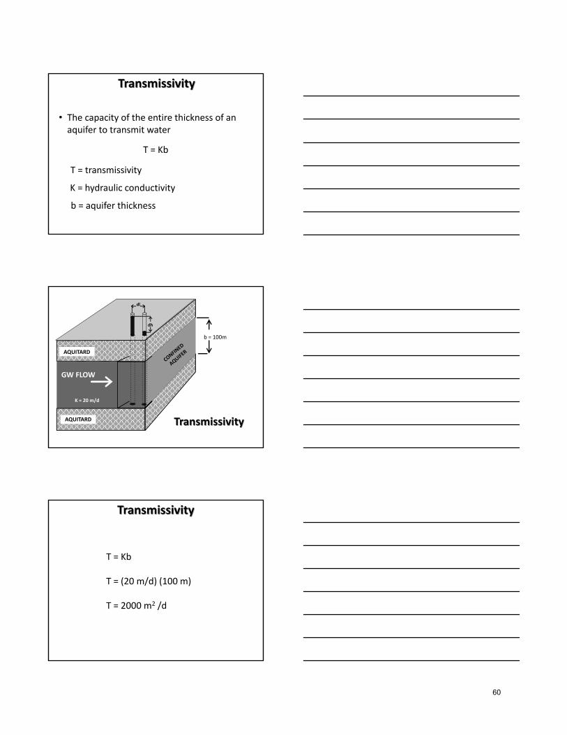
Transmissivity

• The capacity of the entire thickness of an aquifer to transmit water

T = transmissivity

K = hydraulic conductivity

b = aquifer thickness

T = Kb

AQUITARD

AQUITARD

dh

dl

GW FLOW

K = 20 m/d

Transmissivity

b = 100m

Transmissivity

T = Kb

T = (20 m/d) (100 m)

T = 2000 m2 /d

60

Storativity

• The amount of water available for "use" in an aquifer (storage coefficient)

• "Specific yield" in an unconfined aquifer

Selected aquifer stress test slides

Cooper ‐ Jacobs Method

• Advantages

– Less time to perform test; consider straight‐line drawdown over one log cycle on the semi log graphical plot

– Only one well required

– Tests larger aquifer volume than slug test

61

Cooper ‐ Jacobs Method

• Disadvantages

– Requires conductivities >10‐2 cm/s

– Tests smaller portion of the aquifer volume than multiple‐well tests

– Must handle discharge water

Cooper ‐ Jacob Semi Log Plot

D

r

a

w

d

o

w

n

Time

←Log   Cycle→

Cooper ‐ Jacob Formulas

T = transmissivity feet squared per day (ft /day)

Q = pump rate (gpm)

Δs= change in drawdown (ft/log cycle)

K = hydraulic conductivity  ft /day

b = aquifer thickness (feet)

T =T

bK =

2

35 Q

Δs

62

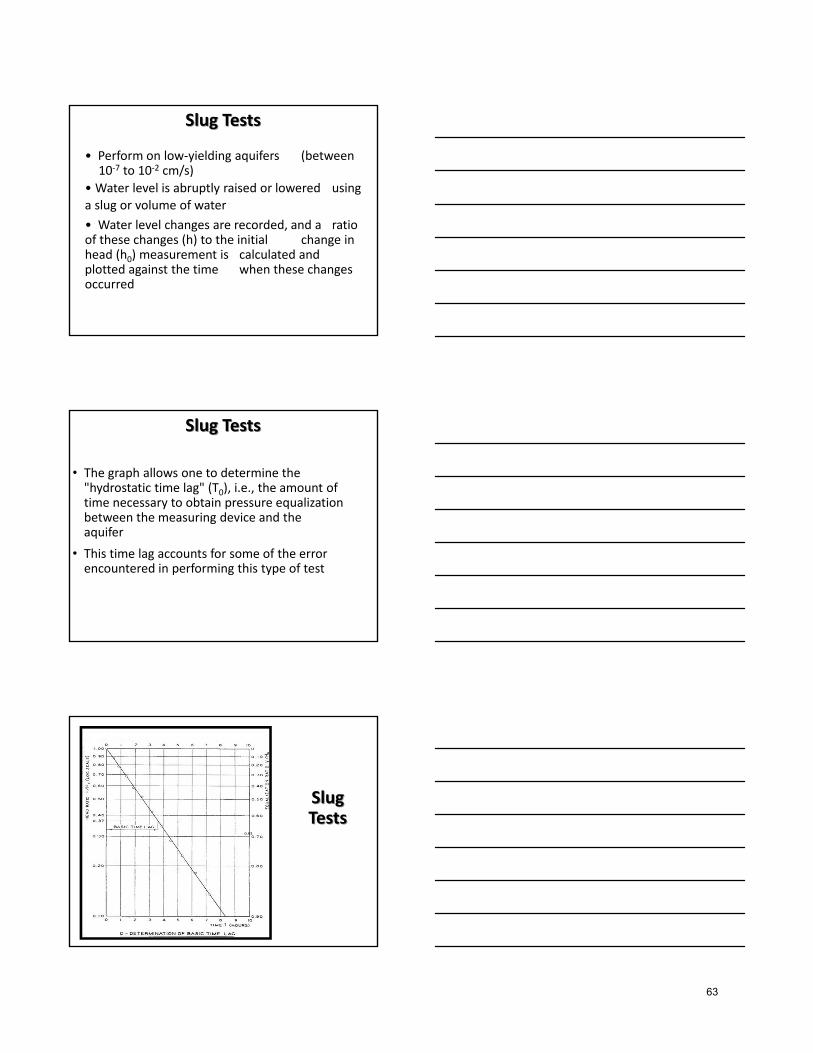
•  Perform on low‐yielding aquifers  (between 10‐7 to 10‐2 cm/s)

• Water level is abruptly raised or lowered  using 

a slug or volume of water

•  Water level changes are recorded, and a  ratio of these changes (h) to the initial  change in head (h0) measurement is  calculated and plotted against the time  when these changes occurred 

Slug Tests

• The graph allows one to determine the "hydrostatic time lag" (T0), i.e., the amount of time necessary to obtain pressure equalization between the measuring device and the aquifer

• This time lag accounts for some of the error encountered in performing this type of test 

Slug Tests

Slug Tests

o.63

63

•Can use small‐diameter well•No pumping = no discharge•Inexpensive = less equipment required•Estimate made in situ•Interpretation/reporting time is shortened

ADVANTAGES

Slug Tests

• Disadvantages

– Very small volume of aquifer tested

– Only apply to low conductivities

– Transmissivity and conductivity only estimates

– Not applicable to large‐diameter wells

– Large errors if well not properly developed

Slug Tests

64

Lecture Notes

______________________________________________________________________ ______________________________________________________________________ ______________________________________________________________________ ______________________________________________________________________ ______________________________________________________________________ ______________________________________________________________________ ______________________________________________________________________ ______________________________________________________________________ ______________________________________________________________________ ______________________________________________________________________ ______________________________________________________________________ ______________________________________________________________________ ______________________________________________________________________ ______________________________________________________________________ ______________________________________________________________________ ______________________________________________________________________ ______________________________________________________________________ ______________________________________________________________________ ______________________________________________________________________

65

Lecture Notes ______________________________________________________________________ ______________________________________________________________________ ______________________________________________________________________ ______________________________________________________________________ ______________________________________________________________________ ______________________________________________________________________ ______________________________________________________________________ ______________________________________________________________________ ______________________________________________________________________ ______________________________________________________________________ ______________________________________________________________________ ______________________________________________________________________ ______________________________________________________________________ ______________________________________________________________________ ______________________________________________________________________ ______________________________________________________________________ ______________________________________________________________________ ______________________________________________________________________ ______________________________________________________________________

66

Lecture Notes

______________________________________________________________________ ______________________________________________________________________ ______________________________________________________________________ ______________________________________________________________________ ______________________________________________________________________ ______________________________________________________________________ ______________________________________________________________________ ______________________________________________________________________ ______________________________________________________________________ ______________________________________________________________________ ______________________________________________________________________ ______________________________________________________________________ ______________________________________________________________________ ______________________________________________________________________ ______________________________________________________________________ ______________________________________________________________________ ______________________________________________________________________ ______________________________________________________________________ ______________________________________________________________________

67

Lecture Notes

______________________________________________________________________ ______________________________________________________________________ ______________________________________________________________________ ______________________________________________________________________ ______________________________________________________________________ ______________________________________________________________________ ______________________________________________________________________ ______________________________________________________________________ ______________________________________________________________________ ______________________________________________________________________ ______________________________________________________________________ ______________________________________________________________________ ______________________________________________________________________ ______________________________________________________________________ ______________________________________________________________________ ______________________________________________________________________ ______________________________________________________________________ ______________________________________________________________________ ______________________________________________________________________

68

Lecture Notes

______________________________________________________________________ ______________________________________________________________________ ______________________________________________________________________ ______________________________________________________________________ ______________________________________________________________________ ______________________________________________________________________ ______________________________________________________________________ ______________________________________________________________________ ______________________________________________________________________ ______________________________________________________________________ ______________________________________________________________________ ______________________________________________________________________ ______________________________________________________________________ ______________________________________________________________________ ______________________________________________________________________ ______________________________________________________________________ ______________________________________________________________________ ______________________________________________________________________ ______________________________________________________________________

69

Lecture Notes

______________________________________________________________________ ______________________________________________________________________ ______________________________________________________________________ ______________________________________________________________________ ______________________________________________________________________ ______________________________________________________________________ ______________________________________________________________________ ______________________________________________________________________ ______________________________________________________________________ ______________________________________________________________________ ______________________________________________________________________ ______________________________________________________________________ ______________________________________________________________________ ______________________________________________________________________ ______________________________________________________________________ ______________________________________________________________________ ______________________________________________________________________ ______________________________________________________________________ ______________________________________________________________________

70

Lecture Notes

______________________________________________________________________ ______________________________________________________________________ ______________________________________________________________________ ______________________________________________________________________ ______________________________________________________________________ ______________________________________________________________________ ______________________________________________________________________ ______________________________________________________________________ ______________________________________________________________________ ______________________________________________________________________ ______________________________________________________________________ ______________________________________________________________________ ______________________________________________________________________ ______________________________________________________________________ ______________________________________________________________________ ______________________________________________________________________ ______________________________________________________________________ ______________________________________________________________________ ______________________________________________________________________

71

Lecture Notes

______________________________________________________________________ ______________________________________________________________________ ______________________________________________________________________ ______________________________________________________________________ ______________________________________________________________________ ______________________________________________________________________ ______________________________________________________________________ ______________________________________________________________________ ______________________________________________________________________ ______________________________________________________________________ ______________________________________________________________________ ______________________________________________________________________ ______________________________________________________________________ ______________________________________________________________________ ______________________________________________________________________ ______________________________________________________________________ ______________________________________________________________________ ______________________________________________________________________ ______________________________________________________________________

72

Lecture Notes

______________________________________________________________________ ______________________________________________________________________ ______________________________________________________________________ ______________________________________________________________________ ______________________________________________________________________ ______________________________________________________________________ ______________________________________________________________________ ______________________________________________________________________ ______________________________________________________________________ ______________________________________________________________________ ______________________________________________________________________ ______________________________________________________________________ ______________________________________________________________________ ______________________________________________________________________ ______________________________________________________________________ ______________________________________________________________________ ______________________________________________________________________ ______________________________________________________________________ ______________________________________________________________________

73

Lecture Notes

______________________________________________________________________ ______________________________________________________________________ ______________________________________________________________________ ______________________________________________________________________ ______________________________________________________________________ ______________________________________________________________________ ______________________________________________________________________ ______________________________________________________________________ ______________________________________________________________________ ______________________________________________________________________ ______________________________________________________________________ ______________________________________________________________________ ______________________________________________________________________ ______________________________________________________________________ ______________________________________________________________________ ______________________________________________________________________ ______________________________________________________________________ ______________________________________________________________________ ______________________________________________________________________

74