ii. exact solution of the boltzmann equation in an … · boltzmann equation. the physics and the...
TRANSCRIPT
Nonlinear dynamics from the relativistic Boltzmann equation in theFriedmann-Lemaıtre-Robertson-Walker spacetime
D. Bazow,1 G. S. Denicol,2, 3 U. Heinz,1 M. Martinez,1 and J. Noronha4
1Department of Physics, The Ohio State University, Columbus, OH 43210, USA2Instituto de Fısica, Universidade Federal Fluminense, UFF, Niteroi, 24210-346, RJ, Brazil
3Department of Physics, Brookhaven National Laboratory, Upton, New York 11973-50004Instituto de Fısica, Universidade de Sao Paulo, C.P. 66318, 05315-970 Sao Paulo, SP, Brazil
(Dated: December 13, 2016)
The dissipative dynamics of an expanding massless gas with constant cross section in a spatiallyflat Friedmann-Lemaıtre-Robertson-Walker (FLRW) universe is studied. The mathematical prob-lem of solving the full nonlinear relativistic Boltzmann equation is recast into an infinite set ofnonlinear ordinary differential equations for the moments of the one-particle distribution function.Momentum-space resolution is determined by the number of non-hydrodynamic modes included inthe moment hierarchy, i.e., by the truncation order. We show that in the FLRW spacetime the non-hydrodynamic modes decouple completely from the hydrodynamic degrees of freedom. This resultsin the system flowing as an ideal fluid while at the same time producing entropy. The solutions tothe nonlinear Boltzmann equation exhibit transient tails of the distribution function with nontrivialmomentum dependence. The evolution of this tail is not correctly captured by the relaxation timeapproximation nor by the linearized Boltzmann equation. However, the latter probes additionalhigh-momentum details unresolved by the relaxation time approximation. While the expansion ofthe FLRW spacetime is slow enough for the system to move towards (and not away from) localthermal equilibrium, it is not sufficiently slow for the system to actually ever reach complete localequilibrium. Equilibration is fastest in the relaxation time approximation, followed, in turn, bykinetic evolution with a linearized and a fully nonlinear Boltzmann collision term.
PACS numbers: 25.75-q, 51.10.+y, 52.27.Ny, 98.80.-kKeywords: relativistic Boltzmann equation, thermalization, nonlinear dynamics, FLRW universe.
I. INTRODUCTION
The Boltzmann equation is the main theoretical frame-work for studying the dissipative out-of-equilibrium dy-namics of dilute gases. Within this approach, the trans-port and thermodynamic properties of matter are un-derstood in terms of the one-particle distribution func-tion whose phase-space evolution is determined by theBoltzmann equation. The physics and the mathemat-ics involved in the non-relativistic Boltzmann equationhave been thoroughly studied [1, 2] and, in certain limits,analytical solutions of this nonlinear integro-differentialequation are known.
For instance, Bobylev [3], Krook, and Wu (BKW) [4, 5]derived an exact solution of the Boltzmann equation thatdescribes the nonlinear relaxation of a non-expanding,non-relativistic homogeneous gas with elastic cross sec-tion inversely proportional to the relative speed. For thiscase it was shown that a generic solution to the Boltz-mann equation can be obtained in terms of the momentsof the distribution function whose temporal evolution isdictated by a coupled set of nonlinear ordinary differen-tial equations. A remarkable feature of the BKW solu-tion is the formation of transient high energy tails dueto the nonlinear mode-by-mode coupling among differentmoments of the distribution function. These high energytails show how high energy moments of the distributionare populated over time, a process that directly affectsthe relaxation of the distribution function towards global
equilibrium.The relativistic generalization of the Boltzmann equa-
tion is an active topic of research that has applications indifferent areas of physics, ranging from thermal field the-ory [6–12] to high-energy nuclear collisions [13–24], cos-mology [25–30] and astrophysics [31–34]. A major topicof interest in relativistic kinetic theory is to quantify therole of nonlinear effects in rapidly expanding plasmas,which requires a careful analysis of the type of interac-tions between the constituent particles of the system thatdefines the collision kernel. In practice, this kinetic equa-tion is solved numerically, although it is possible to findexact solutions of the relativistic Boltzmann equation forhighly symmetric systems using the relaxation time ap-proximation as a model for the collision term [27, 35–40] that describes the relaxation of the system to itsequilibrium state with a single microscopic time scale.These exact solutions have been extremely useful to un-derstand certain features of the thermalization process inrelativistic gases while also providing nontrivial ways totest the accuracy and precision of numerical algorithmsfor solving the Boltzmann equation and macroscopic hy-drodynamic approximations to the microscopic kineticevolution[36, 37, 40–43].
However, a complete understanding of the dissipativedynamics of an expanding gas can only be achieved bysolving the full nonlinear Boltzmann equation which nec-essarily embodies an entire hierarchy of microscopic re-laxation time scales and includes mode-by-mode couplingeffects. For instance, it has been shown that nonlinear
arX
iv:1
607.
0524
5v2
[he
p-ph
] 1
2 D
ec 2
016
2
effects play an important role in the hydrodynamiza-tion process of the quark gluon plasma at weak cou-pling [24, 44–55] and in the reheating process of infla-tionary cosmology [56–64]. While these effects have beenstudied only numerically, it would be extremely useful toalso investigate the nonlinear out-of-equilibrium dynam-ics of rapidly expanding systems analytically where thisis possible.
The first step towards this goal was taken in [65] byrecasting the general relativistic Boltzmann equation,in a spatially homogeneous and isotropically expand-ing Friedmann-Lemaıtre-Robertson-Walker (FLRW) uni-verse, in terms of ordinary nonlinear differential equa-tions for the energy moments of the distribution func-tion. There these moment equations were solved analyt-ically for a very specific far-from-equilibrium initial con-dition, and the corresponding distribution function wasfound. This led to a new class of analytical solutions ofthe relativistic Boltzmann equation. Moreover, as ob-served in [65], the symmetries of the FLRW spacetimerestrict the energy momentum tensor to ideal fluid form,whether or not the system is in local thermal equilibrium.The macroscopic hydrodynamic quantities (energy den-sity, temperature, and hydrodynamic flow) thus evolveaccording to the laws of ideal fluid dynamics while thesystem, if initialized in a non-equilibrium state, producesentropy. This provides an explicit counter example to thefolklore that a system must be in local thermal equilib-rium for the hydrodynamic currents to exhibit ideal fluidbehavior.
In this paper we obtain semi-analytical (numerical) so-lutions to the moment equations in FLRW spacetime forvarious initial conditions, to arbitrary accuracy. Thesenew solutions are used to investigate the domain of ap-plicability of two widely used approximation schemes forthe Boltzmann equation: the linearized Boltzmann colli-sion term and the relaxation time approximation. Sucha study not only gives insight into the physical featuresneglected in these two approximations but it also illus-trates how mode-by-mode nonlinear coupling dynamicsmanifests itself within the relativistic Boltzmann equa-tion.
This article is organized as follows: In Sec. II A webriefly review some of the basic properties of the FLRWmetric and introduce our notation. In the rest of Sec. IIwe provide a detailed derivation of the general methodthat allows one to find exact solutions to the nonlinearBoltzmann equation in the FLRW spacetime. We refer toour previous result [65] in Sec. III where we re-derive anexact solution to the Boltzmann equation valid for a spe-cific far-from-equilibrium initial condition. We discussthe entropy production of this system in Sec. IV. Resultsfrom numerical studies involving the different evolutionschemes for the distribution function and the mode-by-mode coupling effects are shown in Sec. V. A summary ofour findings and some general conclusions are presentedin Sec. VI. Some technical details of the calculations canbe found in the appendices.
II. EXACT SOLUTION OF THE BOLTZMANNEQUATION IN AN FLRW SPACETIME
The existence and uniqueness of a solution to the rel-ativistic Boltzmann equation in the spatially flat FLRWspacetime has been demonstrated in Refs. [66, 67]. How-ever, until Ref.[65], no explicit analytical solution wasknown. Building on the work performed in Ref.[65], wehere continue to study nonlinear effects in the Boltzmannequation for an expanding gas of massless particles. Ourstarting point is the Boltzmann equation for a relativis-tic massless gas that expands isotropically and homoge-neously in a FLRW spacetime. We replace the Boltz-mann equation by an infinite hierarchy of equations forits moments – a set of coupled ordinary differential equa-tions for moments of the distribution function. This hier-archy can then be solved, for any initial condition and toan arbitrary precision, by truncation at an appropriateorder. Finally, the distribution function may be recon-structed from the moments.
A. Notation and some properties of FLRWspacetime
The FLRW metric is a solution to Einstein’s equationsdescribing a spatially homogeneous and isotropically ex-panding universe [25, 26, 28, 68]. For a spatially flatuniverse the FLRW metric reads
ds2 = dt2 − a2(t) γij dxi dxj (1)
where i, j ∈ 1, 2, 3, γij is the spatial metric of the 3-dimensional space, and a(t) is a dimensionless scale fac-tor accounting for the expansion that is determined bysolving Einstein’s equations. The general form of γij de-pends on the choice of coordinates; in this work, we usespatial Cartesian coordinates, γij = δij .
1 The determi-nant of this metric is g ≡ det(gµν) = −a6(t) such that√−g= a3(t).The FLRW metric (1) is invariant under the following
transformation:
xi → xi/λ , a(t)→ λ a(t) (2)
and, due to this scaling symmetry, one can set a(t0) = 1at the initial time t0 (which we choose as t0 = 0). Thiswill be our boundary condition for the scaling factor.
We denote the scalar product between 4-vectors,aµ, bµ, as a · b ≡ aµb
µ. For massless particles
1 The FLRW metric (1) is not the most general metric for a max-imally symmetric space. For instance, in a spatially curved 3-space with constant Gaussian curvature K the line element ofFLRW spacetime is given in polar coordinates by
ds2 = dt2 − a2(t)
[dr2
1−K r2+ r2 dΩ2
].

3
with 4-momentum kµ, the on-shell condition, k · k= 0,yields k0 = a(t)
√(k1)2+(k2)2+(k3)2 where (k1, k2, k3) ≡
(kx, ky, kz) is the usual 3-momentum, given by the spatialcontravariant components of the 4-vector kµ. Following[69, 70] we find it convenient to express this instead interms of the magnitude k of a 3-vector k ≡ (k1, k2, k3)constructed from the covariant spatial components ki ofthe 4-momentum, k=
√k21+k22+k23. In terms of k the
on-shell condition for massless particles reads
k0 = k/a(t). (3)
This way of expressing k0 is rather convenient since, aswe shall see in the following section, the factor a(t) inEq. (3) will cancel in the exponent of the equilibriumBoltzmann distribution function.
Furthermore, the Lorentz-invariant momentum spaceintegration measure in curved spacetime is [69, 70]
√−g d4k ≡
√−g dk0dk1dk2dk3 =
dk0dk1dk2dk3√−g
, (4)
while the Lorentz-covariant 3-momentum integrationmeasure over on-shell distributions can be written as∫
k
≡√−g
(2π)3
∫2θ(k0) δ(k·k−m2) dk0dk1dk2dk3
=
∫dk1dk2dk3
(2π)3k0√−g≡ 1(
2πa(t))3 ∫ d3k
k0, (5)
where the last equality defines our notation d3k ≡dk1dk2dk3 in terms of the covariant spatial componentsof the momentum four-vector. Using spherical coordi-nates, this reduces for massless particles to∫
k
=1
(2π)3
∫ ∞0
k dk
a2(t)
∫dΩk, (6)
with k as defined above.
B. The relativistic Boltzmann equation in FLRWspacetime
The general relativistic Boltzmann equation for an on-shell single-particle distribution function f(x, k) is givenby [27, 29, 69, 70]
kµ(uµD+∇µ
)f(x, k) + kλk
µΓλµi∂f(x, k)
∂ki= C[f ], (7)
where C[f ] is the nonlinear collision term for binary col-lisions, and Γλµν = 1
2gλγ (∂µgγν+∂νgγµ−∂γgµν) are the
Christoffel symbols. In (7) we have decomposed thespace-time derivative ∂µ into its temporal and spatialcomponents in the comoving frame, ∂µ =uµD+∇µ, withD≡uν∂ν , ∇µ≡∆µν∂
ν . Here, uµ = (1, 0, 0, 0) is the 4-velocity of the comoving frame and ∆µν ≡ gµν − uµuν
the projection operator onto the spatial components inthis frame.2
The symmetries of the system restrict the number ofindependent variables upon which the distribution func-tion can depend [35–39]. In our case, the homogeneityof the FLRW spacetime (1) implies that, in the comov-ing frame, the distribution function f(x, k) → f(t, k)is independent of the spatial coordinates and is spher-ically symmetric in momentum space [28, 71]. For ageneral collision kernel, we define the shorthand nota-tion fk(t) ≡ f(t, k) for the distribution function and theBoltzmann equation in FLRW spacetime thus reads3
(u · k)Dfk = C[f ] , (8)
where, in the comoving frame, u · k = k0 = k/a(t).For a single particle species with classical Boltzmann
statistics, the collision term C[f ] takes the form [29]
C[f ] =1
2
∫k′pp′
Wkk′→pp′ (fpfp′ − fkfk′) , (9)
where Wkk′→pp′ is the transition rate and∫p
is defined
as in Eq. (5) in terms of the covariant spatial componentsof the momentum p in the comoving frame. The transi-tion rate can be written in terms of the differential crosssection σ(s,Θ) as follows [29, 69, 70]:
Wkk′→pp′ = s σ(s,Θs) (2π)6√−g δ4(k+k′−p−p′). (10)
Here the total energy s and the scattering angle Θs aregiven by
s = (k+k′) · (k+k′), cos Θs =(k−k′) · (p−p′)(k−k′) · (k−k′)
. (11)
The transition rate Wkk′→pp′ in (10) is a Lorentz scalarand obeys the detailed balance and crossing symmetriesWkk′→pp′ = Wpp′→kk′ =Wkk′→p′p [29, 72].
For simplicity we here assume isotropic scattering, i.e.,the differential cross section depends only on s. Then wecan express the transition rate through the total crosssection σT (s)≡π
∫dΘs sin Θs σ(s,Θs),
4 and the Boltz-mann equation in the FLRW spacetime (8) can be writ-ten as
(u · k)Dfk = Cgain − Closs, (12)
2 Note that even though a fluid filling a FLRW universe homoge-neously is locally static, the expanding FLRW geometry inducesa nonzero fluid expansion rate θ(t) ≡ ∂µ(
√−g uµ)/
√−g = 3H(t)
where g = −a6(t) is the determinant of the FLRW metric andH(t) = a(t)/a(t) is the Hubble parameter.
3 In the comoving frame the only non-zero Christoffel symbols areΓ0ij = a(t)a(t) δij and Γi0j = δij H(t). For the FLRW spacetime,
the term in (7) involving the Christoffel symbols thus cancelsexactly:
kλkµΓλµi
∂fk
∂ki=(
Γ0ji + gljΓ
l0i
)k0 kj
∂fk
∂ki= 0 .
4 Note that, due to the indistinguishability of the two particles, weintegrate here only over half the solid angle, i.e. over 2π.

4
with the gain and loss terms
Cgain =(2π)5
2
∫k′pp′s σT (s)
√−g δ4(k+k′−p−p′) fpfp′ , (13a)
Closs =(2π)5
2
∫k′pp′s σT (s)
√−g δ4(k+k′−p−p′) fkfk′ . (13b)
In the following subsections we replace all of the physi-cal information contained in the Boltzmann equation (anonlinear integro-differential equation for the distribu-tion function fk) by a set of equations for the energymoments of the distribution function.
C. Normalized energy moments and theirevolution equations
We define the energy moments ρn of the distributionfunction as follows5
ρn(t) =
∫k
(u · k)n+1 fk =1
2π2
∫ ∞0
dk kn+2
an+3(t)fk. (14)
The positivity of the distribution function implies thatρn(t) ≥ 0. The number and energy densities are givenby ρ0(t) and ρ1(t), respectively. The higher-order mo-ments ρn≥2(t) do not have an intuitive macroscopic in-terpretation but are needed to resolve additional micro-scopic details of the system. Moments of lower ordern correspond to softer momentum modes (longer wave-lengths) while moments of higher-order probe the shortwavelength structure of the local distribution function.
The collision kernel in (9) conserves particle number,energy, and momentum. In an FLRW spacetime the cor-responding moments ρ0(t) and ρ1(t) evolve by the follow-ing equations [68]:
Dρ0(t) + 3ρ0(t)H(t) = 0 , (15a)
Dρ1(t) + 4ρ1(t)H(t) = 0 . (15b)
Equations (15) follow from Einstein’s equations for a ho-mogeneous and isotropic fluid in an FLRW metric. Theycorrespond to the equations of motion of an ideal fluid,dµj
µµ = dµT
µν = 0 (where dµ denotes the covariant deriva-tive), with particle current jµ(t) =n(t)uµ and energy-momentum tensor Tµν(t) = e(t)
(43u
µuν− 13gµν). Equa-
tions (15) are solved by
ρ0(t) =n0a3(t)
=1
a3(t)
λ0T30
π2, (16a)
ρ1(t) =e0a4(t)
=1
a4(t)
3λ0T40
π2, (16b)
5 In kinetic theory, it is usually assumed that the distribution func-tion fk belongs to the Hilbert space L2(0,∞), i.e., the space ofsquare-integrable functions defined in the interval k ∈ (0,∞)[3, 29, 73]. In this case, it is then guaranteed that the momentsρn (14) are finite.
where n0 ≡ ρ0(0) and e0 ≡ ρ1(0) are the initial parti-cle and energy densities, and T0 and λ0 are the initialtemperature and fugacity assigned to the system. Thetemperature and fugacity of our nonequilibrium systemare obtained from the matching conditions
ρ0(t) = neq(t) =λ(t)T 3(t)
π2, (17a)
ρ1(t) = eeq(t) =3λ(t)T 4(t)
π2. (17b)
By comparing Eqs. (16) and (17) we find λ= constantand T (t) =T0/a(t), such that the local equilibrium dis-tribution function has the following form (remember thatu · k = k/a(t) in the comoving frame)
f eqk = λ(t) e−u·k/T (t) = λ e−k/T0 . (18)
One sees that, when f eqk is expressed in terms of the mag-nitude k of the covariant spatial components of the mo-mentum four-vector, its dependence on a(t) completelycancels (hence f eqk is time independent).6 For later con-venience we also introduce the energy moments of theequilibrium distribution function:
ρeqn (t) ≡∫k
(u · k)n+1 f eqk (t) =(n+2)!
2π2λTn+3(t) . (19)
We now use the Boltzmann equation to derive the setof equations of motion satisfied by the energy momentsρn(t). To this end we apply the comoving time derivativeD to the definition of ρn and substitute the resulting timederivative of the distribution function Dfk from Eq. (12).This results in the following evolution equation for themoments ρn:
Dρn(t) + (3 + n)H(t)ρn(t) = C(n)gain(t)− C(n)loss(t) , (20)
where the nth moments of the loss and gain terms, C(n)loss
and C(n)gain, respectively, are given by the following expres-sions:
C(n)loss =(2π)5
2
∫kk′pp′
s σT (s) (u · k)n
×√−g δ4(k+k′−p−p′) fkfk′ , (21a)
C(n)gain =(2π)5
2
∫kk′pp′
s σT (s) (u · p)n
×√−g δ4(k+k′−p−p′) fkfk′ . (21b)
6 The physics of this is the following [26, 68]: A comoving observerdefines the physical 3-momentum of a massless particle via theenergy-momentum relation k0 = Ephys = |kphys|. The discus-sion in Sec. II A shows that this physical 3-momentum kphys isrelated to the covariant spatial components of the momentum4-vector by kphys = k/a(t), and its magnitude kphys is relatedto the magnitude k of the covariant components of the momen-tum four-vector by kphys = k/a(t). Hence k/T0 = kphys/T (t) =Ephys/T (t) where T (t) = T0/a(t) is the cosmologically redshiftedtemperature of the expanding FLRW universe as seen by the co-moving observer.

5
For an energy independent total cross section σT (s) =const (“hard sphere approximation”) the integrals inEq. (21) can be done analytically (see Appendix A), withthe result
C(n)loss(t) = σT ρn(t)ρ0(t) , (22a)
C(n)gain(t) = 2σT
n∑m=0
(n+2)n!
(m+2)!(n−m+2)!ρn−m(t)ρm(t) .
(22b)
Substituting these results in Eq. (20) one obtains thefollowing set of coupled evolution equations for the mo-ments ρn, which is equivalent to the Boltzmann equation:
Dρn(t) + (3+n)H(t)ρn(t) + σT ρ0(t)ρn(t)
= 2σT
n∑m=0
(n+2)n!
(m+2)!(n−m+2)!ρn−m(t)ρm(t) .
(23)
The conservation laws (15) are recovered by setting n= 0and n= 1, respectively.
Defining the normalized moments
Mn(t) =ρn(t)
ρeqn (t), (24)
and substituting them into Eq. (23) one obtains a similarinfinite nonlinear hierarchy of coupled ordinary differen-tial equations for the Mn moments:
a3(t ) ∂tMn(t ) +Mn(t ) =1
n+1
n∑m=0
Mm(t )Mn−m(t ).
(25)Here we defined the dimensionless time variable t = t/`0where `0 = 1/(σTn0) is the mean free path at t= 0.
The solution of this infinite set of nonlinear coupleddifferential equations (25) contains the same physical in-formation as the original Boltzmann equation. At thelevel of moments, the nonlinear dependence of the col-lision kernel on the distribution function is encoded inthe mode-by-mode coupling between moments of differ-ent order, as seen on the r.h.s. of Eq. (25). The conser-vation laws (15) together with the matching conditionsimply that the only non-evolving moments are M0(t) andM1(t):
M0(t) = M1(t) = 1 for all t. (26)
It is convenient to further express the time dependenceof the moments in terms of the variable
τ(t)
=
∫ t
t0
dt′
a3(t′)(27)
since it absorbs all the information about the expansionof the universe (i.e., the scale parameter a(t)). In thiscase, the hierarchy of moment evolution equations (25)becomes
∂τMn(τ ) +Mn(τ ) =1
n+1
n∑m=0
Mm(τ )Mn−m(τ ). (28)
Interestingly enough, this equation exactly coincides withthe moment equation originally derived by Bobylev [3],Krook, and Wu [4, 5] for a non-relativistic, spatially ho-mogeneous and isotropic, non-expanding gas (see Eq.(35) in Ref. [5]). The fact that the non-equilibriumdynamics of both physical systems is governed by thesame moment equations is intriguing since the underly-ing symmetries of the two problems are quite different.BKW’s derivation is based on Galilean invariance whileours is embedded into general relativity. One shouldnote, however, that the relation between the momentsMn and the distribution function fk differs in the twocases: equations (14) and (24) here are replaced in thenon-relativistic case by Eqs. (18) and (21) in Ref. [5].
Let us mention some important properties of the mo-ment equations (28). First, the equation of motion (28)implies that if Mn(0) > 0 for all n (which is true for anypositive definite initial distribution function fk(0)) thenMn(τ) will remain positive for τ ≥ 0. Equation (28)shows that the nth moment couples only to moments ofthe same or lower order. Therefore, for a given set ofinitial values for the moments Mn(0) (or a given initialdistribution function fk(0)) we can express the solutionMn(τ) by a recursive procedure in terms of the solutionsMm(τ) of lower order moments m < n. This can beseen explicitly by writing the general solution of Eq. (28)formally as
Mn(τ) = Mn(0)e−ωnτ (29)
+1
n+1
n−1∑m=1
∫ τ
0
dτ ′ eωn(τ′−τ)Mm(τ ′)Mn−m(τ ′) ,
where
ωn = 1− 2
n+ 1=n− 1
n+ 1. (30)
If rotational symmetry is broken, the evolution equationfor Mn includes additional couplings to moments of orderm > n, rendering a recursive solution impossible [29, 46,74–76].
At sufficiently large times τ all moments Mn(τ) ap-proach unity, independently of their initial condition.This can be seen explicitly by finding the fixed pointsof the set of equations (28), i.e., by studying the con-dition ∂τMn(τ)
∣∣τ=τmax
= 0, where τmax = limt→∞ τ(t).
When imposing this condition on Eq. (28) we obtain thefollowing recursion relation:
Mn(τmax) =1
n− 1
n−1∑m=1
Mm(τmax)Mn−m(τmax) . (31)
This algebraic equation can be solved recursively as fol-lows: the matching conditions that define temperatureand fugacity impose that M0(τmax) = M1(τmax) = 1.This gives immediately M2(τmax) = 1 for n= 2. Induc-tion shows that if Mm(τmax) = 1 for m < n then alsoMn(τmax) = 1 and, consequently, the stationary point of

6
(28) is given uniquely by Mn(τmax) = 1, for all values ofn. In an FLRW universe, the Boltzmann equilibrium dis-tribution is therefore the only fixed point of the Boltz-mann equation. This analysis does not tell us whetheror not the fixed point is an attractor; however, the valid-ity of the H-theorem in FLRW spacetime [28] necessarilyguarantees that the equilibrium is stable. The numeri-cal simulations reported below show that the equilibriumdistribution is a stable (attractive) fixed point of Eq. (12).
D. Reconstructing the distribution function fromLaguerre moments
So far, the solution of the Boltzmann equation, fk(τ),has been viewed as a function of the normalized energymoments Mn(τ). In practice it is, however, easier toreconstruct the distribution function from its momentsif one uses a different set of moments, defined througha basis of orthogonal polynomials [74]. In this paper weuse the Laguerre basis [46] (see Appendix B) in whichthe distribution function can be written as
fk(τ) = f eqk
∞∑n=0
cn(τ)L(2)n
(u · kT (τ)
), (32)
where the Laguerre moments cn(τ) are given by
cn(τ) =2
(n+1)(n+2)
1
ρ0(τ)
∫k
(u · k)L(2)n
(u · kT (τ)
)fk
=
n∑r=0
(−1)r(n
r
)Mr(τ) . (33)
The second equality in this equation makes use of theclosed form (B1) of the Laguerre polynomials. For theLaguerre moments the particle number and energy con-servation laws imply that
c0(τ) = 1, c1(τ) = 0 for all τ (34)
(see Eq. (26)). The relation between cn and Mn can beinverted with the help of the binomial inverse transfor-mation identity [77]:
Mn(τ) =
n∑r=0
(−1)r(n
r
)cr(τ) . (35)
In Appendix C we show that the Laguerre momentscn obey exactly the same hierarchy of coupled ordinarydifferential equations as the normalized moments Mn:
∂τ cn(τ ) + cn(τ ) =1
n+1
n∑m=0
cm(τ )cn−m(τ ) . (36)
Only the initial conditions look different when expressedin terms of Mn or cn.
The structure of these equations has an interestingfeature: since the right-hand side couples only to mo-ments of lower order, one cannot generate low-order mo-ments dynamically from higher-order ones. If initially
all Laguerre moments up to order nmin vanish such thatcnmin
is the lowest nonvanishing moment at τ = 0, itwill remain the lowest nonvanishing moment at all times.This is useful when reconstructing the distribution func-tion. Additionally, we note that the approach to thermalequilibrium fk → f eqk is characterized by Mn(τ)→ 1 forall n and, consequently, cn(τ)→ δn0. Also, using thatc0(τ) = 1 and c1(τ) = 0 one finds that (36) can be rewrit-ten as
∂τ cn(τ ) + ωncn(τ ) =1
n+1
n−2∑m=2
cm(τ )cn−m(τ ) , (37)
which will be useful in the next section when we discussthe linearized approximation for the collision kernel.
Similar to the generic solution for the normalized en-ergy moments Mn (29), for n ≥ 2 Eq. (37) admits asolution which for generic initial conditions reads as
cn(τ) = cn(0)e−ωnτ (38)
+1
n+1
n−2∑m=2
∫ τ
0
dτ ′ eωn(τ′−τ) cm(τ ′) cn−m(τ ′) ,
The first term on the RHS corresponds to the linear con-tribution from the collision term (cf. Eq. (45) in the fol-lowing subsection) and decays exponentially with a rateωn that increases with n according to Eq. (30). The non-linear second term describes the mode-by-mode couplingof cn with moments of lower order. For small devia-tions from equilibrium (cn 1 for all n 6= 0, 1) the lin-ear, exponentially decaying terms dominate the dynam-ical evolution of the distribution function. For initiallylarge deviations from equilibrium, however, no generalstatement can be made as to which of the two terms (lin-ear or nonlinear) controls the evolution at early times.Bounds on the nonlinear contribution to the generic so-lution of the Laguerre moments have been discussed fornon relativistic systems [78]. As we will see further be-low, at late times all cn eventually become small, andthe remaining evolution is then controlled by the lin-ear first term in Eq. (38), i.e. if τl is large enough themoments cn relax for τ > τl exponentially with rate ωn,cn(τ > τl) ≈ cn(τl) e
−ωn(τ−τl).In addition to the particle number and energy conser-
vation laws c0(τ) = 1 and c1(τ) = 0, Eq. (38) yields thefollowing exact solutions for the lowest order Laguerremoments (shown here up to n= 5):
c2(τ) = c2(0)e−ω2τ , c3(τ) = c3(0)e−ω3τ ,
c4(τ) = c4(0)e−ω4τ + 3 c22(τ)[e−(ω4−2ω2)τ−1
], (39)
c5(τ) = c5(0)e−ω5τ + 2 c2(τ)c3(τ)[e−(ω5−ω2−ω3)τ−1
].
One can see that mode-by-mode coupling among the La-guerre moments may start already at n = 4, while forn < 4 the moments are either linear or completely deter-mined by conservation laws. Another interesting feature
7
of (36) is related to parity: if initially all the moments offk with odd Laguerre polynomials vanish, c2n+1(0) = 0,the recursive nature of (36) implies that this remains trueat all times: c2n+1(τ) = 0 ∀ t. The same does not holdfor initial conditions that have nonzero moments onlywith odd Laguerre polynomials. In this case, even La-guerre moments will in general be generated dynamicallyby mode-coupling between odd Laguerre moments, e.g.c6(τ) = 1
2c23(τ)
(e2τ/7−1
). This requires the full nonlin-
ear collision term and hence does not happen when thelatter is linearized as in the following subsection.
Finally, one sees from Eq. (32) that the distributionfunction at zero momentum f(τ, 0) is finite at all times aslong as the sum of the Laguerre moments remains finite.We will see later that at large times all Laguerre momentsapproach zero exponentially, rendering mode-couplingterms negligible for τ 1. However, mode-coupling ef-fects may be important if initial conditions are such thatnonlinear terms, such as c2(τ)2e−(ω4−2ω2)τ in (39), be-come of the same order as the linear contributions, inthis case ∼ c4(0)e−ω4τ . So while the moments decayexponentially at long times, their amplitudes in generalstill contain information about the nonlinear mode cou-pling at early times that cannot be obtained in linearizedapproaches such as the ones discussed in the next twosubsections.
E. Moment evolution for a linearized Boltzmanncollision term
Systems not too far from local thermal equilibrium canbe described macroscopically using viscous hydrodynam-ics. To derive such hydrodynamic equations from theunderlying Boltzmann equation one expands the distri-bution around the local equilibrium one, fk = f eqk +δfk,and linearizes the Boltzmann equation in δfk. When rep-resenting the Boltzmann equation in terms of moments,this procedure corresponds to a linearization of the mo-ment equations around the equilibrium values of the mo-ments Mn = 1 and cn = δn0, respectively:
Mn ≈ M linn = 1 + δMn , (40)
cn ≈ clinn = δn0 + δcn , (41)
with δM0 = δM1 = δc0 = δc1 = 0 due to particle and en-ergy conservation. The corresponding linearized momentevolution equations, obtained from (28) and (37), read
∂τδMn(τ) + ωnδMn(τ) =2
n+1
n−1∑m=2
δMm(τ) , (42)
∂τδcn + ωnδcn = 0 , (43)
with ωn given by Eq. (30). It is easy to check that theselinearized equations respect the relations (33) and (35),to linear order.
The general solution of Eq. (42) is
δMn(τ) = δMn(0)e−ωnτ
+2
n+1
n−1∑m=2
∫ τ
0
dτ ′eωn(τ′−τ) δMm(τ ′) ,
(44)
while Eq. (43) is simply solved by
δcn(τ) = e−ωnτ cn(0). (45)
These equations apply to moments with n≥ 2. One seesthat, in contrast to the linearized energy moments, theequations of motion for the linearized Laguerre momentsdecouple, i.e., the moments δcn are eigenfunctions ofthe linearized collision operator with eigenvalues (decayrates) ωn. The mode with the longest lifetime is the firstnon-hydrodynamic7 mode, n= 2, with τ2 = 1/ω2 = 3. Asalready noted, the decay rates increase with n, approach-ing unity for n→∞.
We can combine Eq. (45) with Eq. (35) to obtain thefollowing alternate solution of the linearized energy mo-ments (44):
δMn(τ) =
n∑r=2
(−1)r(n
r
)cr(0) e−ωrτ . (46)
This form shows that, at asymptotically long times, theexponential decay of all Mn moments is controlled bycnmin
, i.e. by the lowest initially non-vanishing Laguerremoment which has the smallest damping rate ωnmin
.With the solution (45) of the linearized moment equa-
tions one finds the solution of the linearized Boltzmannequation8 for the distribution function as follows (seeEq. (32)) :
f link (τ) = f eqk
[1 +
∞∑m=2
cm(0) e−ωmτL(2)m
( kT0
)](47)
F. Moment evolution in the relaxation timeapproximation
Due to its simplicity, one of the most widely employedmodels for the collision term is the Relaxation Time Ap-proximation (RTA) [79]. For our relativistic system itreads [80]
C[f ] = − u · kτrel(t)
[fk(t)− f eqk
], (48)
7 A non-hydrodynamic mode relaxes within a timescale that re-mains finite in homogeneous systems, in contrast to hydrody-namic modes such as sound waves.
8 In practice, in numerical calculations one truncates the infinitesums by defining a maximum number of terms nmax.
8
where τrel is the scale at which the distribution functionrelaxes to its local equilibrium state. For the FLRW uni-verse, the RTA Boltzmann equation is [27, 28]
∂tfk(t) = −fk(t)− f eqkτrel(t)
, (49)
where according to Eq. (18), f eqk is time independent.In general, the expression for the relaxation time τrel
varies according with the physical process one wants toinvestigate. For instance, the typical timescale for energyand momentum transport in the shear and bulk channelsof relativistic fluids are in general different (this is thecase in weak coupling QCD [81]). A physical prescriptionmust be given in order to meaningfully compare resultscompared within RTA and other evolution schemes. Inthis paper we choose to define τrel in such a way that theshear viscosity to entropy density ratio of the gas, η/s,computed within RTA agrees with the result found usingthe full Boltzmann equation for massless particles withconstant cross section [46]. This condition fixes
τrel(t) = αa3(t)`0 (50)
with α = 1.58375.9 In this case, RTA Boltzmann equa-tion becomes
α∂τfk(τ) = f eqk − fk(τ) , (52)
which is easily solved analytically:
fRTAk (τ) = f eqk + e−τ/α(fk(0)− f eqk
)(53)
where fk(0) is the distribution function at τ = 0. Substi-tuting this solution into the expression for the energy andLaguerre moments of the distribution function, we obtainthe following analytic expressions for these quantities:
cRTAn (τ) = cn(0)e−τ/α , (54)
MRTAn (τ) = 1 + e−τ/α
(Mn(0)− 1
). (55)
As before, we have MRTA0 =MRTA
1 = cRTA0 (0) = 1 andcRTA1 = 0 for all τ , due to the conservation laws.
Whereas for the linearized collision term studied inthe preceding subsection each moment cn relaxes withits own decay rate ωn = (n−1)/(n+1), we see that theRTA collision term causes all of them to relax at thesame decay rate 1/α. Since in the RTA the collisionterm is characterized by the single time scale τrel, this is
9 The relaxation time was calculated from the Boltzmann equationfor massless particles interacting with constant isotropic crosssection in Ref. [46, 82]:
τrel =5
4
η
ρeq0 (t)T (t). (51)
Here η= 1.267T/σT is the shear viscosity. Eq. (50) is obtainedby using this value of η together with ρeq0 (t) = n0/a3(t) in (51).
perhaps not unexpected. On the other hand, linearizingthe full Boltzmann collision term still leaves us with aninfinite hierarchy of collision time scales, causing each ofthe Laguerre moments δcn (45) to decay at its own rateωn. One sees that by requiring η/s computed in RTAto match the result from the full Boltzmann equation,the decay rate in RTA 1/α ∼ 0.631413 comes to lie inbetween ω4 and ω5.
We will show numerical comparisons between the so-lutions of the full nonlinear Boltzmann equation, its lin-earized form, and the RTA later in Sect. V. In the follow-ing section, however, we first use the methods developedin this section to rederive the exact analytical solution ofthe nonlinear Boltzmann equation presented in a previ-ous publication [65].
III. AN EXACT ANALYTIC SOLUTION OFTHE BOLTZMANN EQUATION WITH
NONLINEAR COLLISION KERNEL
A. τ-evolution of the distribution function and itsmoments
One can see by inspection that Eq. (28) admits thefollowing analytic solution of BKW type, valid for alln ≥ 0 and τ ≥ 0 [65]:
Mn(τ) = nKn−1(τ)− (n−1)Kn(τ), (56)
K(τ) = 1 − 1
4e−τ/6 . (57)
Inserting the moments above into Eq. (33) gives the cor-responding analytic solution of Eq. (36) for the Laguerremoments,10
cn(τ) = (1−n)(1−K(τ)
)n= cn(0)e−nτ/6, (59)
where the initial values for the Laguerre moments are
cn(0) =1− n
4n, (60)
which can be obtained from the initial condition for theenergy moments in (56):
Mn(0) =
(3
4
)n (1 +
n
3
). (61)
In Ref. [65] we noted that the Fourier transform of thedistribution function can be expressed in terms of thenormalized energy moments and used this to construct
10 This makes use of the combinatorial identity
n∑r=0
(−1)r(nr
) [rxr−1 − (r−1)xr
]= (1−n) (1−x)n . (58)

9
the corresponding exact analytic solution for the distri-bution function from Mn as given in (56). This methodis generalizable to any solution of the Boltzmann equa-tion whose Fourier transform exists. Here we rederive thesame analytic solution for fk from the Laguerre moments,using the orthogonality and completeness of the Laguerrepolynomials. Inserting the analytic solution (59) for theLaguerre moments into the decomposition (32) and us-ing the relations (B3) and (B4) listed in Appendix B weobtain
fk(τ) = f eqk
∞∑n=0
(1−n) (1−K(τ))n L(2)
n (k/T0) (62)
=λ e−k/(K(τ)T0)
K4(τ)
[4K(τ)− 3 +
k
K(τ)T0
(1−K(τ)
)].
This agrees with Eq. (22) in [65]. This analytic solu-tion of the nonlinear Boltzmann equation is obtained forthe following far-from-equilibrium initial conditions forthe distribution function (with energy and Laguerre mo-ments given in (60,61)):
fk(0) = λ256
243
(k
T0
)exp
(−4
3
k
T0
), (63)
The out-of-equilibrium initial condition in (63) gives theopportunity to study how different approximations forthe collision kernel affect the behavior of the Laguerremoments in an analytical manner. While all the evolu-tion schemes correctly give exponentially decaying cn’s,for the RTA solution in (55) all the moments decay withthe same scale 1/α (given by the choice for the relax-ation time). In the solution for the Laguerre momentsobtained by linearizing the collision kernel in (45) eachmoment decays exponentially at a distinct rate given bythe eigenvalues of the collision operator, which shouldbe in general a much better approximation to the multitimescale solution of the full nonlinear case in Eq. (59).We note, however, that for the exact solution studiedin this section, the linearized collision kernel approachconsiderably underestimates the decay rates of the mo-ments in which n is large. This occurs because for thelinearized moments (45) one finds limn→∞ cn(τ)/cn(0) =e−τ while taking the same large n limit in (59) giveslimn→∞ cn(τ)/cn(0) = limn→∞ e−nτ/6 → 0.11
In Fig. 1 we show the evolution of the the normalizedmoments Mn (56) (left panel) and the Laguerre moments
11 Note that Eq. (59) implies that for this exact analytical solutionall modes with n> 6 decay faster than any of the eigenmodes ωnof the linearized collision operator, even at late times when all de-viations from equilibrium cn (n≥ 2) are small. This exemplifiesto the extreme the consequences of non-linear mode-coupling ef-fects in the full Boltzmann collision operator. By linearizing thecollision operator one loses essential information that is neededto describe correctly the dynamical evolution of the Laguerremoments for the exact solution (59,60).
cn (59) (right panel) as a function of the dimensionlessvariable τ . At τ = 0 the normalized moments Mn de-crease monotonically with increasing n. This means thatthe softest modes of the system are initially more stronglypopulated than the harder ones, albeit not thermallyequilibrated (i.e. they are < 1). The initial values forthe Laguerre moments cn (59) are negative and increase(i.e. their magnitude decreases) with increasing n. BothMn and cn are seen to increase monotonically with timeτ (i.e. the magnitudes of cn decrease monotonically), ap-proaching their equilibrium values 1 and 0, respectively,at τ →∞.
This is more clearly seen in Fig. 2 where we plotthe ratio F (τ, k/T0) = fk(τ)/f eqk between the out-of-equilibrium solution (62) and its equilibrium value asa function of k/T0 for different values of τ . This ratiomeasures the deviation of the system from local equilib-rium. At τ = 0 moderately soft modes with momenta1.5 . k/T0 . 5 are overpopulated while the longest andshortest wavelength modes k/T0 < 1.5 and k/T0 > 5 areunderpopulated.
As time proceeds the distribution function approachesequilibrium: the initial overpopulation at intermediatemomenta quickly decreases, filling in first the “hole” atsmall momenta and only later the strong initial depletionat large momenta. At τ = 12 the distribution function isseen to be essentially thermalized up to k& 5T0, witha residual depletion of the high-momentum tail that in-creases with k.
Thermalization of the high-momentum modes appearsto require transporting energy from low to high momenta,similar to the “bottom-up” scenario in QCD [83] whereinteractions between the hard modes and the thermalbath created by the soft modes allows the system toeventually reach global thermal equilibrium asymptot-ically. The main difference between the QCD case andthe one at hand is that in the former the high-momentummodes are initially over-occupied whereas here the ini-tial conditions of the analytic solution imply an ini-tial under-population at high momenta. We will see inSec. V that the relatively slow thermalization of the high-momentum part of the distribution function arises frommode-by-mode-coupling effects characteristic of the non-linear Boltzmann collision term with its broad spectrumof microscopic relaxation time scales. This feature is notshared by the relaxation time approximation where colli-sions are controlled by a single, common, relaxation time.
B. A finite τ-horizon caused by cosmic expansion
In the previous sections it was convenient to use the di-mensionless variable τ (defined in Eq. (27)) as a time-likeparameter in the evolution equations for the momentsMn and cn. This was a key ingredient in demonstratingthe relation between our approach and the BKW solu-tion. In this subsection we translate the results obtainedso far back into the original coordinate system, using the

10
M0, M1
M5
M15
M25
M50
0 5 10 15 20 25 30
0.0
0.2
0.4
0.6
0.8
1.0
τ
Mn(τ
)
(a)
C1
C2
C3
C4
C5
0 5 10 15 20
-0.06
-0.04
-0.02
0.00
τ
Cn(τ
)
(b)
FIG. 1: (Color online) Evolution of the normalized moments Mn (56) (panel (a)) and the Laguerre moments cn (59) (panel(b)) as a function of the dimensionless time variable τ .
time variable t.
The dynamics of the cosmic expansion is encoded inthe scale factor a(t) of the FLRW metric (1). Its func-tional form is determined from Friedmann’s equation anddepends on the equation of state [25, 26, 28]. For aconformal equation of state consistent with our study ofmassless particles, the exact solution for the scale factora(t) defined in Eq. (1) reads [25, 26]:
a(t) =
√1 + br t , br = 2H0
√Ωr, (64)
where H0 is the Hubble parameter evaluated at the initialtime t0 = 0 and Ωr is the dimensionless density parame-ter associated with radiation. Equation (27) then relatesτ with t as follows:
τ =2
br
(1− (br t+ 1)−
12
). (65)
This implies that the infinite t interval 0 ≤ t < ∞ is
τ = 0
τ = 4
τ = 8
τ = 12
0 5 10 15 20 25 30 35 40 45 50
0.0
0.2
0.4
0.6
0.8
1.0
k /T0
F(τ
,k/T
0)
FIG. 2: (Color online) Ratio between the out-of-equilibriumsolution (62) and the equilibrium distribution as a functionof k/T0.
mapped on a finite τ interval 0 ≤ τ ≤ τmax where
τmax = limt→∞
τ(t) =2
br. (66)
Consequently, the limit of perfect local thermalizationof the distribution function at τ → ∞ is never reached:while (in contrast to the Gubser expansion studied in thecontext of relativistic heavy-ion collisions [36, 37, 84]) amassless gas in equilibrium in FLRW spacetime wouldremain so despite the expansion of the universe, its cos-mic expansion is not slow enough to allow the system toever reach complete local thermal equilibrium if it is ini-tially out of equilibrium, fk(0) 6= f eqk . Instead, the sys-tem approaches a quasi-stationary off-equilibrium statecharacterized by the distribution
limt→∞
fk(t) = fk(τmax) (67)
=λ e−k/Tlim
K4max
[4Kmax − 3 +
k
Tlim
(1−Kmax
)].
Here we defined the “limiting temperature” Tlim =KmaxT0, with Kmax = 1 − 1
4 exp [−τmax/6].12 Figure 2shows that this spectrum is suppressed at high mo-menta relative to the asymptotic thermal distributionλ exp(−k/T0). The large-k tail of the distribution is es-sentially exponential, with inverse slope parameter start-ing at 3
4T0 at time t= 0 and increasing with time until it
reaches Tlim = KmaxT0 at time t→∞. Kmax approaches1 as the initial Hubble constant (initial cosmic expansionrate) H0 approaches zero.
12 Recall that in terms of the physical momentum kphys seen bya comoving observer we have k = a(t)kphys such that k/Tlim =kphys/Tlim(t) where Tlim(t) ≡ Tlim/a(t) is the time-dependent(cosmologically redshifted) “limiting temperature” seen by thatobserver. Since the temperature seen by the comoving ob-server keeps redshifting we characterize the state (67) as quasi-stationary.

11
IV. ENTROPY PRODUCTION BYNON-HYDRODYNAMIC MODES
The entropy density current Sµ defined in terms of thesingle particle distribution function in FLRW
Sµ ≡ −∫k
kµ fk (ln fk−1) (68)
obeys Boltzmann’s H-theorem [28], i.e. dµSµ ≥ 0, with
the equality only being satisfied in equilibrium. Becauseof the symmetries of FLRW, one can write Sµ = s uµ
with
s = −∫k
(u · k) fk (ln fk−1) (69)
being the entropy density. Defining S = a3s and noticingthat a6 dµS
µ = ∂τS, we find (using the decomposition(32))
∂τS = −n02
∞∑n=2
hn(τ)∂τ cn(τ) (70)
where
hn(τ) =
∫ ∞0
dxx2e−xL(2)n (x) ln
(1+
∞∑m=2
cm(τ)L(2)m (x)
).(71)
Equation (70) shows that entropy production onlyceases when the Laguerre moments become time inde-pendent, i.e., when equilibrium is reached. The low-est order moments c0 and c1, associated with hydrody-namic modes, do not participate in the entropy produc-tion which is entirely given by the non-hydrodynamicdegrees of freedom cn≥2. In FLRW spacetime, localequilibrium is an attractor of the Boltzmann equation,i.e., a system initially prepared in local equilibrium willremain in local equilibrium (in spite of the cosmologi-cal expansion) while an initially non-equilibrated systemwill evolve towards local equilibrium, producing entropyalong the way. What is different from other situationsis that the evolution of the macroscopic hydrodynamicobservables such as the energy and particle number den-sities follows the laws of ideal fluid dynamics even if thesystem is out of equilibrium. This happens because, inthe present situation which has an exceptional degree ofsymmetry, the non-hydrodynamic modes completely de-couple from the energy momentum tensor, thereby pre-serving its ideal fluid form. Similar systems were studiedbefore in [38, 39].
In dissipative fluid dynamics entropy production is ex-pressed in terms of the non-equilibrium corrections tothe energy-momentum tensor and particle 4-current. Forexample, in the widely used Israel-Stewart formulationof dissipative fluid dynamics [75], entropy productionis expressed in terms of the shear stress tensor πµν asdµS
µ = πµνπµν/(2ηT ), where η is the shear viscosity.The shear stress tensor reflects the excitation of non-hydrodynamic modes of the Boltzmann equation [46, 82],
and such a formulation is expected to work if the sys-tem is sufficiently close to thermodynamic equilibrium.However, the entropy production derived in (70) can ob-viously never be expressed in a hydrodynamic form evenif the system is close to equilibrium. Therefore, the typeof system discussed here gives an example in which thesymmetries of the system always forbid the descriptionof dissipative processes (such as entropy production) interms of the laws of fluid dynamics.
Based on the discussion above, one can use (37) to findanother expression for the entropy production
∂τS =n02
[ ∞∑n=2
ωn hncn −∞∑n=2
hnn+1
n−2∑m=2
cn−mcm
]. (72)
This expression shows that, at late times when the La-guerre moments cn are small, entropy production in thefull nonlinear case (in which the moments follow (37))should be very well approximated by the correspondingexpression computed in the linearized Boltzmann colli-sion approximation. In fact, one can expand the loga-rithm in (71) to linear order to find
hn(τ) = (n+1)(n+2) cn(τ) +O(c2n) (73)
and, thus,
∂τS =n02
∞∑n=2
(n+1)(n+2)ωnc2n(τ) +O(c3n). (74)
In this limit the fact that entropy increases with timeis manifest, and each moment is seen to contribute toentropy production an amount proportional to its de-cay rate. If the higher order corrections in Eq. (74) aresmall (as they are for the initial conditions studied in thiswork), one expects that the linearized Boltzmann colli-sion approximation should give an accurate descriptionof the entropy produced in the full nonlinear problem.This is confirmed in the numerical studies performed inSection V C. Also, using (73) one finds that
S(τ) = Seq −n04
∞∑n=2
(n+1)(n+2) c2n(τ) + . . . (75)
where Seq is the corresponding equilibrium expression.This shows explicitly that the maximum entropy value isachieved in equilibrium.
Equation (72) expresses the entropy production interms of the time evolution of the Laguerre moments ofthe distribution function. In Sec. II we studied their evo-lution for the full nonlinear Boltzmann collision terms aswell as for a linearized version and for the relaxation timeapproximated collision term. In the next section we willshow numerical results for these different types of micro-scopic evolution. Following the production of entropy ineach of these three cases will yield valuable insights intothe dynamics that underlies the thermalization processesin the Boltzmann equation.
12
V. NUMERICAL RESULTS
In this section we compare the solutions to the fullnonlinear Boltzmann equation (32), its linearized ver-sion (47) and the RTA (49). For simplicity we assumethat the fugacity is λ = 1. We consider the followinginitial conditions of the distribution function fk(0), theLaguerre moments cn(0), and the normalized momentsMn(0):
• The exact solution initial condition (ES-IC) alreadygiven in Eqs. (59)-(61):
fk(0) = λ256
243
(k
T0
)e−
43
kT0 , (76a)
cn(0) =1− n
4n, (76b)
Mn(0) =
(3
4
)n (1 +
n
3
). (76c)
• The one mode initial condition (1M-IC):
fk(0) = λ e−kT0
[1 +
3
10L(2)2
(k
T0
)], (77a)
cn(0) = δn0 +3
10δn2 (77b)
Mn(0) = 1 +3
10
(n
2
). (77c)
• The two-mode initial condition (2M-IC):
fk(0) = λ e−kT0
[1− 1
10L(2)3
(k
T0
)(78a)
+1
20L(2)4
(k
T0
)], (78b)
cn(0) = δn0 −1
10δn3 +
1
20δn4 , (78c)
Mn(0) = 1 +1
10
(n
3
)+
1
20
(n
4
). (78d)
All of these initial conditions satisfy the requirementMn(0) ≥ 0 for all n, which ensures positivity of the dis-tribution function fk. Notice also that for 1M-IC (77)and 2M-IC (78) the normalized moments Mn(0) divergewhen n→∞, which should be contrasted with the ES-ICcase(63) where Mn(0) vanishes in this limit.
In this section we will compare for each of these initialconditions the evolution of the moments of the distribu-tion function, the phase-space evolution of the distribu-tion function reconstructed from the Laguerre moments,and the amount of entropy produced in the evolution, forthe evolution schemes defined by the full nonlinear Boltz-mann collision kernel, its linearized version, and also therelaxation time approximation.
A. Evolution of the moments
The infinite set of differential equations (28) for thenormalized moments Mn is truncated at a finite nmax
and then solved numerically. The evolution of the lin-earized moments M lin
n = 1 + δMn is obtained by solvingthe differential equations (42) for δMn, with initial con-ditions fixed by δMn(0) = Mn(0) − 1. Within the RTAthe evolution of the moments MRTA
n is determined byEq. (55).
Figure 3 shows the numerical solutions for the mo-ments M10 (left column) and M20 (right column) as func-tions of the dimensionless variable τ for the three initialconditions listed above. We observe that the differencebetween the values of the moments Mn, M lin
n , and MRTAn
gets larger as one increases the order n of the moment.Since higher-order moments are more strongly weightedat higher momenta, these differences indicate that theRTA and the linear approximation of the Boltzmann col-lision term provide descriptions of the microscopic dy-namics that degrade at short distance scales.
At large times, all Mn moments relax exponentially totheir equilibrium value of 1. In the insets in Fig. 3 weplot the difference between Mn(τ) and their asymptoticvalue on a logarithmic scale, in order to visualize the rateof approach to equilibrium of each moment. We see thatin RTA the moments MRTA
n relax much faster to theirasymptotic value than for both the full and linearizedBoltzmann collision terms. In RTA all modes relax ex-ponentially at the same rate ω = 1/α (defined by ourchoice for the relaxation time) while for both the full andlinearized Boltzmann collision term the energy momentsMn mix Laguerre moments of different orders that decaywith different rates ωn < 1. At large times τ , their decayis dominated by the moment with the smallest decay rate,namely the first non-vanishing non-hydrodynamic modenmin. For ES-IC and 1M-IC, the lowest non-vanishingnon-hydrodynamic mode is c2, and correspondingly forboth the full and linearized Boltzmann collision termsthe Mn modes decay asymptotically with ω2 = 1/3. For2M-IC the lowest non-vanishing non-hydrodynamic modeis c3, and correspondingly for both the full and linearizedBoltzmann collision terms the Mn modes decay asymp-totically somewhat faster, with ω3 = 1/2. We also notethat at large times the deviations of the moments fromtheir asymptotic values become small, and the time evo-lutions of the linearized and full moments converge.
At early times the faster relaxation of the MRTAn mo-
ments to their equilibrium values compared to their re-laxation for the full and linearized collision term is mostevident. However, Fig. 3 also shows that for some ofthe initial conditions the early-time evolution of the Mn
moments exhibits dramatic differences even between thefull and linearized collision terms. These differences arisefrom mode coupling effects which are generically largeas long as the moments Mn deviate strongly from theirequilibrium values.
We point out that for the initial condition ES-IC the

13
Exact
Linear
RTA
0 5 10 15 20 25
-1.4
-1.0
-0.6
-0.2
0.2
0.6
1.0
τ
M10
(τ)
(a)
ES-IC
6 8 10 12 14
-4
-3
-2
-1
0
τlo
g 10|M
10(τ
)-1|
0 5 10 15 20 25-5.0
-4.2
-3.4
-2.6
-1.8
-1.0
-0.2
0.6
τ
M20
(τ)
(b)
ES-IC
6 8 10 12 14
-4
-3
-2
-1
0
τ
log 1
0|M
20(τ
)-1|
0 5 10 15 20 25
1
3
5
7
9
11
13
15
τ
M10
(τ)
(c) 1M-IC
5 10 15
-4
-3
-2
-1
0
1
τ
log 1
0|M
10(τ)-
1|
0 5 10 15 20 250
25
50
75
100
τM
20(τ
)
(d) 1M-IC
5 10 15
-4
-3
-2
-1
0
1
τ
log 1
0|M
20(τ)-
1|
0 5 10 15 20 25
0
5
10
15
20
25
τ
M10
(τ)
(e) 2M-IC5 10 15
-3
-2
-1
0
1
τ
log 1
0|M
10(τ)-
1|
0 5 10 15 20 250
50
100
150
200
250
300
350
τ
M20
(τ)
(f ) 2M-IC
5 10 15-3
-2
-1
0
1
τ
log 1
0|M
20(τ)-
1|
FIG. 3: (Color online) Evolution of the moments M10 (left column) and M20 (right column) as a function of the dimensionlesstime τ according to the nonlinear evolution equation (28), its linearized version (42), and within the RTA (55) for the ES-IC (76)(panels (a)-(b)), 1M-IC (77) (panels (c)-(d)), and 2M-IC (78) (panels (e)-(f)). See text for further details.
moment M lin20 becomes negative at early times, specifi-
cally in the interval 0 . τ . 7 (see panel (b) in Fig. 3).13
From their definition it is clear that this cannot hap-pen for a distribution function that is positive definite.This dynamical behavior resulting from the linearizationof the moments around their thermal equilibrium valuesis thus unphysical. We will see later that, for the initialconditions of the exact solution discussed in Sec. III, thisunphysical dynamics causes the distribution function toturn negative at large momenta as time proceeds, some-what reminiscent of a similar phenomenon observed forthe exact solution of the RTA Boltzmann equation in asystem undergoing Gubser expansion [36, 85].
13 We have checked numerically that for 20≤n≤ 100 all the mo-ments M lin
n turn negative somewhere in the interval τ ∈ (0, 7).
In Fig. 4 we present the logarithm of the magnitudeof the Laguerre moments |cn| as a function of n for a setof fixed τ values, τ = 0.5, 4, 8 for the left, middle andright column, respectively, and for the initial conditionsmentioned above. As shown in Eqs. (39), the solutionsfor the moments with n ≤ 3 are the same in the nonlin-ear case as in the linearized Boltzmann approximation,and this is observed in Fig. 4. For the ES-IC at earlytimes there is basically no distinction among the differ-ent evolution schemes (since the initial cn are alreadyall nonzero while nonlinear mode-coupling effects havenot yet had a chance to manifest themselves). As timeevolves the cn’s with large n quickly distinguish nonlin-ear evolution (red circles) from linear evolution schemes(denoted by the blue triangles and green squares); how-ever, only at late times can clearly distinguish (especiallyat large n) between the results from the RTA and the lin-earized Boltzmann approach.

14
2 3 4 5 6 7 8 9 10 11 12 13 14 15-18
-14
-10
-6
-2
n
log 10
|cn(τ
)|
(a )
τ = 0.5ES-IC
Exact
Linear
RTA
2 3 4 5 6 7 8 9 10 11 12 13 14 15-18
-14
-10
-6
-2
n
log 10
|cn(τ
)|
(b )
τ = 4ES-IC
2 3 4 5 6 7 8 9 10 11 12 13 14 15
-18
-14
-10
-6
-2
n
log 10
|cn(τ
)|
(c )
τ = 8ES-IC
2 3 4 5 6 7 8 9 10 11 12 13 14 15-12
-10
-8
-6
-4
-2
0
n
log 10
|cn(τ
)|
(d )
τ = 0.51M-IC
2 3 4 5 6 7 8 9 10 11 12 13 14 15-10
-8
-6
-4
-2
0
n
log 10
|cn(τ
)|
(e )
τ = 41M-IC
2 3 4 5 6 7 8 9 10 11 12 13 14 15-10
-8
-6
-4
-2
0
n
log 10
|cn(τ
)|
(f )
τ = 81M-IC
2 3 4 5 6 7 8 9 10 11 12 13 14 15
-10
-8
-6
-4
-2
0
n
log 10
|cn(τ
)|
(g )
τ = 0.52M-IC
2 3 4 5 6 7 8 9 10 11 12 13 14 15
-10
-8
-6
-4
-2
0
n
log 10
|cn(τ
)|
(h )
τ = 42M-IC
2 3 4 5 6 7 8 9 10 11 12 13 14 15
-10
-8
-6
-4
-2
0
n
log 10
|cn(τ
)|
(i )
τ = 82M-IC
FIG. 4: (Color online) Evolution of the Laguerre moments as a function of n according to the nonlinear Boltzmann equation(red circle), linear approximation (blue triangle) and RTA (green square) for fixed values of τ = 0.5, 4, 8 (left, middle and rightcolumn respectively). For the initial conditions of the distribution function we use the ES-IC (76) (panels (a,b,c)), 1M-IC (77)(panels (d,e,f)), and 2M-IC (78) (panels (g,h,i)).
λ e-k /T0
τ = 0
τ = 2
τ = 4
τ = 8
0 5 10 15 20
-10
-8
-6
-4
-2
0
k / T0
log 1
0f(τ
,k/T
0)
(a)ES-IC
0 5 10 15 20
-10
-8
-6
-4
-2
0
k / T0
log 1
0f(τ
,k/T
0)
(b)1M-IC
0 5 10 15 20
-10
-8
-6
-4
-2
0
k / T0
log 1
0f(τ
,k/T
0)
(c)2M-IC
FIG. 5: (Color online) Snapshots of the full nonlinear distribution function as a function of k/T0 at different values of τ =0, 2, 4, 8 (with fugacity λ = 1). For the initial conditions of the distribution function we use the ES-IC (76) (panel a),1M-IC (77) (panel b), and 2M-IC (78) (panel c).
For the 1M-IC only c0 and c2 are initially nonzero (par-ity even), and one can see that c2n+1(τ) = 0 for all τ , asexplained in Sec. II D. Also, this case clearly shows theeffect of mode-by-mode coupling responsible for excitingfor τ > 0 modes with n > 2 even though they were ini-tially zero,. This should be contrasted with the linearevolution schemes that give cn>2(τ) = 0 for all τ . Thedifference in the decay rate for c2 between the RTA and
the nonlinear (and linearized) case is evident in panel fof Fig. 4.
Since c2(0) = 0 for 2M-IC, Eq. (39) implies that c4(τ)obtained in the nonlinear evolution is identical to the re-sult computed within the linearized Boltzmann approx-imation, i.e. c4(τ) = c4(0)e−ω4τ . This can be seen inFig. 4g,h,i. Once again mode-by-mode coupling in thefull nonlinear evolution is responsible for exciting for 2M-

15
IC moments with n > 4 which become nonzero alreadyafter a short time τ = 0.5. The higher moments can onlybe excited by nonlinear coupling with lower modes whichis an effect not included in either the RTA or the linearBoltzmann approximation.
The Laguerre moments cn contain all the infor-mation about the solutions of the Boltzmann equa-tion. However, the way cn encodes this informationis not at all trivial. For instance, in the deep infraredf(τ, k→ 0) = f eqk
∑∞n=0 cn(τ). Also, the complicated
time evolution of the analytical solution in Eq. (62) istranslated into a simple exponential decay of the La-guerre modes described by (59).
B. Evolution of the distribution function
The recursive structure of the evolution equations (36),(45) and (55) for the Laguerre moments of the distribu-tion function makes it easy to systematically improve thedescription of the distribution function by increasing thetruncation order nmax (the total number of moments)until convergence is achieved.14
1. Evolution of non-thermal energy tails
In Sec. III we saw for the exact analytical solution (62)of the full Boltzmann equation that, while it approachesequilibrium at large τ , hard momenta are being occupiedvery slowly and large deviations from equilibrium persistfor high values of k/T0 at very large τ . Here we study nu-merically how fk(τ) evolves towards equilibrium with thefull nonlinear Boltzmann collision term for the two otherinitial conditions listed at the beginning of this sectionand compare it with the evolution of the ES-IC initialcondition for which we have an exact analytic result.
Figure 5 shows that the other initial conditions cor-respond to initial distribution functions which deviatefrom equilibrium even more strongly than the one cor-responding to the exact solution, albeit in different mo-mentum regions. In these initial conditions hard modesare separated from soft modes by a “kink” (located, e.g.,near k/T0 = 9 for 2M-IC) that is more distinct in the2M-IC case than in the 1M-IC (where it also occurs ata lower value of k/T0). Taking all three panels of thefigure together one observes that the low-momentum re-gion k/T0 . 5 relaxes to equilibrium very quickly, reduc-ing deviations from equilibrium occupancy to below 20%
14 For the initial conditions studied in this work we were able to en-sure convergence of the series (32) at all times with a small num-ber nmax of associated Laguerre polynomials. However, for other(still well-behaved) initial conditions (e.g. a Gaussian bump
added to a thermal distribution) the polynomials L(2)n are notwell-adapted to describe the high-momentum tail of the distri-bution function, and we found it necessary to include a very largenumber nmax of these polynomials to ensure convergence of theseries for fk(τ).
already at τ ∼ 2 while at k/T0> 20 deviations from equi-librium by up to a factor 5 persist up to τ ∼ 10. TheBoltzmann collision terms thus thermalizes the systemdifferentially: first the system reaches approximate equi-librium at thermal length scales whereas thermalizationat sub-thermal length scales takes much longer.
2. Comparing the evolution of the distribution function fordifferent approximations of the collision kernel
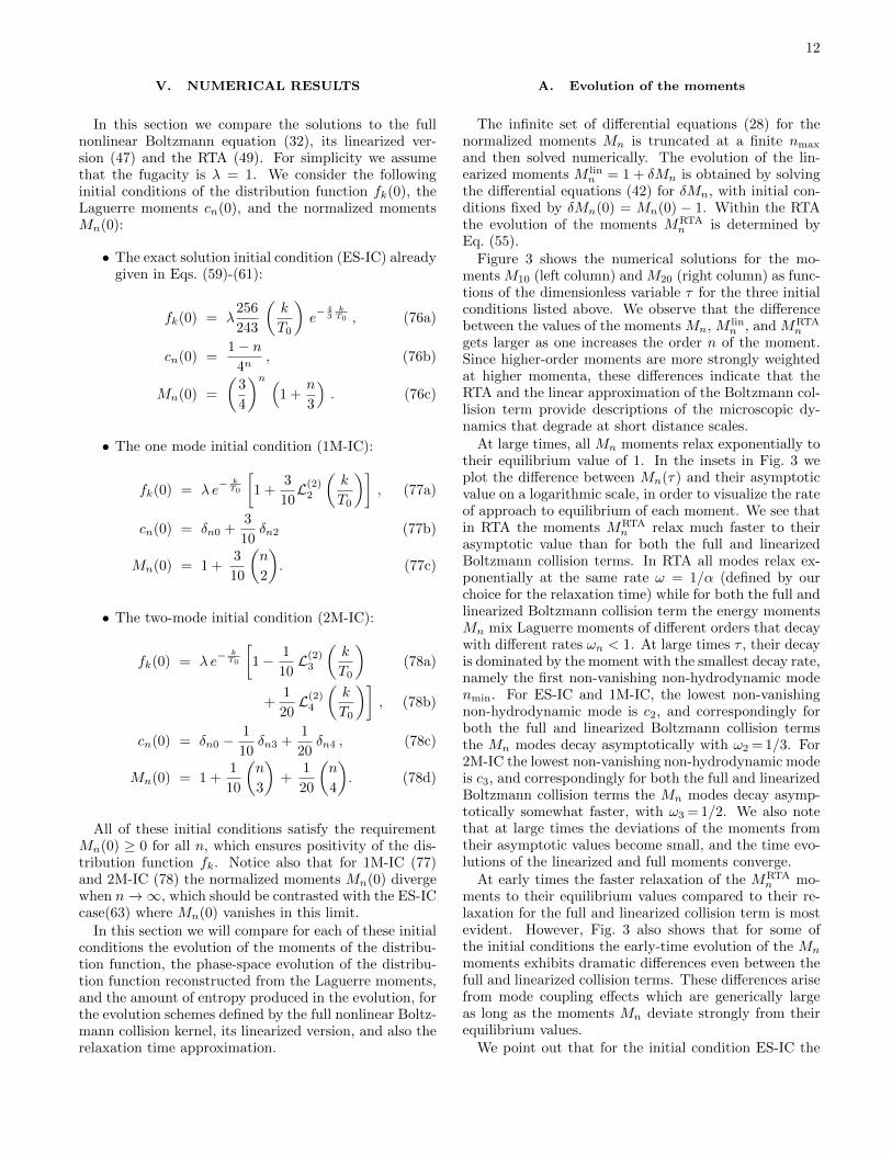
In Figs. 6 and 7 we compare numerical results for thephase-space evolution of the distribution function for thefull nonlinear solution to the Boltzmann equation (32),its linear approximation (47), and the RTA (53) for allthree sets of initial conditions. In Fig. 6 we plot thelogarithm of the ratio F (τ, k/T0)≡ fk(τ)/f eqk (τ) of thenon-equilibrium distribution function to its equilibriumvalue as a function of k/T0, for a set of fixed τ values,τ = 1, 8, 15 (left, middle, and right column). In thefirst row, we plot the magnitude |F | of this ratio be-cause, for the linearized collision term, the distributionfunction evolves to negative values at large momenta astime proceeds. This behavior was already anticipated inSec. V A where we saw that some of the energy momentsMn became unphysically negative when evolved with thelinearized evolution equations. Fig. 6a, b, c shows thatthe pathological region of negative distribution functionsappears to move to larger momenta as time proceeds.This is consistent with the observation that at large τthe deviations from equilibrium get smaller and the lin-ear approximation to the full Boltzmann collision term(which does not cause the distribution function to be-come negative) thus can be expected to work better. Wenote once again that with our choice for the relaxationtime the RTA evolved distribution function reaches equi-librium much more quickly than both the nonlinear caseand the linearized Boltzmann collision approximation;the slowest approach to equilibrium is observed when thesystem is evolved with the full nonlinear collision term.The three lower rows of panels further show that themomentum range in which the dynamically evolved dis-tribution function closely approaches equilibrium growswider, extending to larger momenta as time proceeds.
Figure 7 shows the time evolution of the same ratio Fplotted in 6 at two different momenta (k/T0 = 10 and 20,respectively). Similar to what we saw for the evolutionof its energy moments, one observes a rapid approach tothermal equilibrium in the RTA evolution, compared tothe much slower thermalization found using the nonlin-ear collision term. At the lower of the two selected k/T0values, differences between the time evolution for the fulland the linearized Boltzmann collision term are hardlynoticeable. For the larger k/T0 = 20, the early-time evo-lution differs significantly between the full nonlinear andthe linearized collision terms for ES-IC and 1M-IC; inparticular, for the exact analytic solution the linearizedtime evolution leads to unphysical negative values of thedistribution function at early times.
16
Exact
Linear
RTA
0 5 10 15 20 25 30 35 40 45 50
-4
-3
-2
-1
0
k / T0
log 1
0|F
(τ,k
/T0)|
ES-IC
τ = 1
(a)
0 5 10 15 20 25 30 35 40 45 50
-4
-3
-2
-1
0
k / T0
log 1
0|F
(τ,k
/T0)|
ES-IC
τ = 8
(b)
0 5 10 15 20 25 30 35 40 45 50
-0.15
-0.10
-0.05
0.00
k / T0
log 1
0|F
(τ,k
/T0)|
ES-IC
τ = 15
(c)
0 5 10 15 20 25 30 35 40 45 50
0
1
2
3
4
k / T0
log 1
0F(τ
,k/T
0)
1M-IC
τ = 1(d)
0 5 10 15 20 25 30 35 40 45 50
0
1
2
3
k / T0
log 1
0F(τ
,k/T
0)
1M-IC
τ = 8(e)
0 5 10 15 20 25 30 35 40 45 50
0.0
0.2
0.4
0.6
0.8
1.0
k / T0
log 1
0F(τ
,k/T
0)
1M-IC
τ = 15(f )
0 5 10 15 20 25 30 35 40 45 50
0
1
2
3
4
k / T0
log 1
0F(τ
,k/T
0)
2M-IC
τ = 1(g )
0 5 10 15 20 25 30 35 40 45 50
0.0
0.5
1.0
1.5
2.0
2.5
3.0
k / T0
log 1
0F(τ
,k/T
0)
2M-IC
τ = 8(h)
0 5 10 15 20 25 30 35 40 45 50
0.0
0.2
0.4
0.6
0.8
1.0
k / T0
log 1
0F(τ
,k/T
0)
2M-IC
τ = 15(i )
FIG. 6: (Color online) Snapshots of the ratio F (τ, k/T0)≡ fk(τ)/feqk (τ) as a function of k/T0 for τ = 1, 8, 15 (left, middle
and right column) according to the nonlinear Boltzmann equation (red line), linear approximation (blue dashed line) and RTA(green dotten line). For the initial conditions of the distribution function we use the ES-IC (76) (panels (a,b,c)), 1M-IC (77)(panels (d,e,f)), and 2M-IC (78) (panels (g,h,i)).
At late times, the difference between the value at agiven momentum of the evolving non-equilibrium distri-bution function and its thermal limit decreases exponen-tially. The rate of approach to equilibrium is ω= 1/α inRTA, as is expected because all its Laguerre momentsdecay exponentially with this rate. For the full Boltz-mann collision term, the thermalization rate convergesat late times to ω2 = 1/3 for ES-IC and 1M-IC and toω3 = 1/2 for 2M-IC, i.e. at large times thermalizationis controlled by the lowest (and slowest) non-vanishingnon-hydrodynamic moment (which is n= 2 for ES-IC and1M-IC and n= 3 for 2M-IC). This asymptotic late-timebehavior is universal in the sense that it applies at allmomenta.
C. Entropy production
We quantify the total entropy produced during thethermalization process by the fractional increase
∆S(τ) =S(τ)− S(0)
S(0). (79)
The time evolution of ∆S is studied in Fig. 8 for the threeinitial conditions for the distribution function listed atthe beginning of this section.15 All cases have the sameinitial energy and particle density which evolve accordingto ideal fluid dynamics to the same final equilibrium stateat τ → ∞. What is different in each case is the initialentropy of the system. The different initial conditionscorrespond to non-equilibrium configurations and, thus,their initial entropy is lower than the equilibrium value.Since equilibrium is a global attractor of the dynamics,the relative difference
∆Seq ≡Seq − S(0)
Seq(80)
gives the amount of entropy produced over all time foreach initial condition. We find ∆Seq = 0.51% for ES-IC,
15 We do not show the entropy production for the linearized evolu-tion of the initial conditions ES-IC, Fig (8)a, since this leads tonegative distribution functions in part of momentum space forwhich the entropy integral is not defined.

17
0 5 10 15 20 25
-1.8
-1.4
-1.0
-0.6
-0.2
0.2
0.6
1.0
τ
F(τ
,k/T
0)
5 10 15
-4
-3
-2
-1
0
τk / T0 = 10 ES-IC
(a)
log 1
0|F
(τ,k
/T0)-
1|
0 5 10 15 20 25-5.0
-4.2
-3.4
-2.6
-1.8
-1.0
-0.2
0.6
τ
F(τ
,k/T
0)
5 10 15
-4
-3
-2
-1
0
τk / T0 = 20
(b)
ES-IC
log 1
0|F
(τ,k
/T0)-
1|
0 5 10 15 20 250.51.01.52.02.53.03.54.04.55.05.56.0
τ
F(τ
,k/T
0)
5 10 15
-3
-2
-1
0
1
τk /T0 = 10
(c)
1M-IC
log 1
0|F
(τ,k
/T0)-
1|
0 3 6 9 12 15 18 21 24
0
5
10
15
20
25
30
35
40
45
τF(τ
,k/T
0)
5 10 15
-3
-2
-1
0
1
τ
k /T0 = 20
1M-IC
(d)
log 1
0|F
(τ,k
/T0)-
1|
0 5 10 15 20 250.60
0.65
0.70
0.75
0.80
0.85
0.90
0.95
1.00
τ
F(τ
,k/T
0)
5 10 15
-4
-3
-2
-1
0
1
τ
(e)
k /T0 = 10
2M-IC
log 1
0|F
(τ,k
/T0)-
1|
0 5 10 15 20 250
10
20
30
40
50
60
70
80
90
100
110
120
τ
F(τ
,k/T
0)
5 10 15
-4
-3
-2
-1
0
1
τ
k /T0 = 20
2M-IC(f )
log 1
0|F
(τ,k
/T0)-
1|
FIG. 7: (Color online) (Color online) Evolution of the ratio F (τ, k/T0)≡ fk(τ)/feqk (τ) as a function of τ , for fixed values of
momentum k/T0 = 10 (left column) and k/T0 = 20 (right column), for the full nonlinear (red line), linear (dotted blue line)and RTA collision term (green dotten line). For the initial conditions we use the ES-IC (76) (panels (a,b)), 1M-IC (77) (panels(c,d)), 2M-IC (78) (panels (e,f)).
0 3 6 90.000
0.001
0.002
0.003
0.004
0.005
τ
ΔS(τ
)
(a) ES-IC
0 3 6 90.00
0.01
0.02
0.03
0.04
0.05
τ
ΔS(τ
)
(b) 1M-IC
Exact
Linear
RTA
0 3 6 9
0.001
0.004
0.007
τ
ΔS(τ
)
(c) 2M-IC
FIG. 8: (Color online) Time evolution of the produced entropy as a fraction of its initial value, ∆S(τ) as defined in Eq. (79),for initial conditions (a) ES-IC (76), (b) 1M-IC (77), and (c) 2M-IC (78).
∆Seq = 4.7% for 1M-IC, and ∆Seq = 0.74% for 2M-IC. Thus, we see that 1M-IC is the initial condition that
is the farthest from equilibrium and, consequently, pro-duces the largest amount of entropy during the evolution.

18
As should be expected from the thermalization studiesof the distribution function and its moments in the pre-ceding subsections, the initial rate of entropy productionand the approach of the total entropy towards its finalequilibrated value is fastest in the relaxation time approx-imation. When the kinetic evolution is controlled by thefull or linearized Boltzmann collision term, the rate of en-tropy production slows down to an asymptotic exponen-tial approach at the rate ωnmin = (nmin−1)/(nmin+1),where nmin is the order of the lowest initially non-zeroLaguerre moment of fk. In Fig. 7 one can clearly distin-guish between the different rates towards thermal equilib-rium between panel (b) where initially the lowest nonzeronon-hydrodynamic moment is c2 which relaxes to equi-librium with the rate ω2 = 1/3, and panels (c,d) whereinitially the lowest nonzero non-hydrodynamic momentis c3, which in turn relaxes to equilibrium at a faster rateω3 = 1/2.
As expected from the discussion in Section IV, thereare no noteworthy differences in the entropy productionrate for the full and the linearized Boltzmann collisionterm. High momentum particles are too rare to signif-icantly contribute to the total entropy of the system,which means that long before the high-momentum tailsof the distribution function become thermal the overallentropy production has already essentially ceased. Inother words, the total entropy is dominated by particleswith thermal momenta, and entropy production essen-tially stops when those thermal particles have reachedan equilibrium state.
VI. CONCLUSIONS
In this work we solved the full nonlinear Boltzmannequation for an expanding massless gas with constantcross section in FLRW spacetime. The problem of solv-ing the nonlinear Boltzmann equation is mapped ontosolving recursively a set of coupled ordinary differentialequations of moments of the distribution function. Theprecision of the solution can be improved systematicallyto any desired value by increasing the number of moments(which results in better resolution of the high-momentumtail of the distribution function). The same method canbe applied to the Boltzmann equation with a linearizedcollision term or using the relaxation time approxima-tion (RTA), which allowed us to investigate the impor-tance for the thermalization process of non-linear mode-by-mode couplings inherent in the Boltzmann collisionterm.
The cosmological expansion in FLRW spacetime wasfound to be slow enough to allow the distribution functionto move towards local equilibrium for any initial condi-tion. Local equilibrium is reached in the asymptotic limitτ → ∞ when expressed in the dimensionless time vari-able τ defined in Eq. (27). This asymptotic limit can,however, only be reached for FLRW universes with in-finitesimally small initial values of the Hubble constant.For finite initial expansion rates, the limit t → ∞ in
physical time is reached after a finite interval in τ , whichleaves the distribution function in a non-equilibrium fi-nal state that becomes approximately stationary at latephysical times.
Our work exhibited a characteristic difference betweenthe rates at which the system approaches thermal equi-librium in RTA and for the full or linearized Boltzmanncollision term. For both the full and linearized collisionterms, the asymptotic thermalization rate for the distri-bution function is ωnmin = nmin−1
nmin+1 , which is the dampingrate of the slowest initially occupied non-hydrodynamiceigenmode nmin of the Boltzmann equation. In RTA,on the other hand, if the relaxation time is calculatedwith standard methods using the same (constant) crosssection as in the Boltzmann collision term, the distribu-tion function approaches equilibrium at the larger rateω= 1/α which falls between ω4 and ω5.
The approach to equilibrium is fastest for typical ther-mal momenta whereas the high-momentum tail of thedistribution function takes much longer to thermalize.As time proceeds the window in which the distributionis well approximated by the asymptotic equilibrium dis-tribution widens towards larger momenta. The late ther-malization of the high energy tails is caused by non-linearmode-by-mode couplings that couple higher moments tolower ones and transport energy from low to high mo-menta. It is consistent with the simple intuitive picturethat high-momentum particles require multiple collisionsto thermalize whereas soft particles thermalize alreadyafter a few collisions [5].
Although the dynamics generated by the full collisionterm exhibits non-linear mode-coupling effects, we foundonly very small differences in the evolution towards equi-librium between the full and linearized Boltzmann colli-sion terms as long as we restricted our attention to thedominant thermal momentum region; significant differ-ences between the linear and nonlinear thermalizationdynamics were, however, observed at large momenta orshort length scales. Since high-momentum particles con-tribute very little to the total entropy of the system, therate of entropy production during the thermalization pro-cess was found to be almost indistinguishable between thenonlinear and linearized dynamics. In RTA, however, en-tropy was was found to be produced at much higher rate,leading to faster thermalization.
An interesting aspect of this model is that it com-bines ideal fluid dynamical evolution with dissipation andentropy production. This means that the rate of en-tropy production cannot be expressed in the standardway through dissipative flows (such as the shear stresstensor), which vanish in our model exactly by symme-try. Dissipative effects, while definitely present, do notmanifest themselves hydrodynamically, i.e., they do notaffect the (relatively slow) evolution of the hydrodynamicmodes whose dynamics is controlled by the conservationlaws. For a given initial particle and energy density, theamount of entropy produced depends exclusively on thehow far the initial phase-space distribution is away from

19
thermal equilibrium; all initial configurations with thesame particle and energy density eventually evolve to thesame equilibrium state at τ →∞.
The dramatically different thermalization time scalesfor the RTA and full nonlinear Boltzmann collision termsraise the question whether one could not simply bringthe Boltzmann equation in RTA in congruence with thefull nonlinear Boltzmann equation by appropriate “renor-malization” of the relaxation time τrel used in the RTA.However, this does not work: as our analysis shows, forthe full Boltzmann collision term the relaxation time to-wards thermal equilibrium is not universal, but dependson which of the non-hydrodynamic modes are initiallyoccupied. Thermalization happens asymptotically at therate ωnmin
where nmin is the order of the slowest initiallynon-zero non-hydrodynamic mode. Using in RTA a re-laxation time that depends on the initial condition for thedistribution function (i.e. on which non-hydrodynamicLaguerre moments are initially non-zero) does not makesense.
It will be interesting to try to extend the techniques de-veloped in this work to physically interesting anisotropi-cally expanding systems. Finding an exact solution of thefull nonlinear Boltzmann equation for (0+1)-dimensionalBjorken [86] and/or the (1+1)dimensional Gubser [84]flows in Minkowski space would be of particular practicaland conceptual interest for relativistic heavy-ion physics,and in the cosmological context one would like to be ableto solve the Boltzmann equation in anisotropic space-times such as the Bianchi universes [87]. We leave theseissues for future studies.
Acknowledgements
We gratefully acknowledge inspiring discussions withS. Schlichting, S. Konig, Y. Mehtar-Tani, S. Ozonderand A. Dumitru. MM thanks C. Plumberg for pointingout Ref. [77] on combinatorial identities. JN thanksConselho Nacional de Desenvolvimento Cientıfico e Tec-nologico (CNPq) and Fundacao de Amparo a Pesquisado Estado de Sao Paulo (FAPESP) for financial support.UH and MM express their gratitude to the Institute forNuclear Theory, where part of this work was realized, forits hospitality. GSD was supported by DOE ContractNo. DE-SC0012704. DB, UH and MM are supportedby the U.S. Department of Energy, Office of Science,Office for Nuclear Physics under Award DE-SC0004286.UH, MM, and JN acknowledge support through abilateral travel grant from FAPESP and The Ohio StateUniversity.
Appendix A: Moments of the collision kernel
In this Appendix we describe the procedure to performthe integrals (21) for the case of a constant cross sec-tion. We start by calculating the term C(n)loss (21a). Werecall from Sec. II A that we formulate all momentumintegrals in terms of the covariant components of thefour-momenta. For massless particles in FLRW space-time we have s = (k+k′) · (k+k′) = 2 (1− cos θ) k k′2
and u · k = k0 = k/a(t).
The term C(n)loss (21a) is calculated as follows
C(n)loss =(2π)5
2σT
∫kk′pp′
s (u·k)n
×√−g δ4(k+k′−p−p′) fkfk′ ,
=σTan+2
∫kk′
kn+1 k′ (1− cos θ) fkfk′ (A1)
= σT
[1
2π2
1
an+3
∫ ∞0
dk kn+2 fk
]×[
1
4π2
1
a3
∫ ∞0
dk′ k′2 fk′
∫ 1
−1d(cos θ)(1− cos θ)
]= σT ρn ρ0 .
In the second line we used the identity∫pp′
√−g δ4(k+k′−p−p′) =
1
(2π)5, (A2)
and in the last equality we recalled the definition (14) ofthe energy moments. This completes the computational
details of the loss term C(n)loss (21a).
The calculation of C(n)gain (22a) is harder. Let us start
by rewriting Eq. (22a) as follows
C(n)gain =(2π)5
2σT
∫kk′
s fkfk′ Pn , (A3)
where we define the scalar quantity
Pn =
∫p p′
(u·p)n√−g δ4(k+k′−p−p′) . (A4)
We calculate Pn in the center of mass frame wherek+k′= 0, where k = (k1, k2, k3) is constructed from thecovariant spatial components of the 4-vector kµ. (Thesame applies to all 3-vectors below, see discussion inSec. II A.) In this frame the total energy of the systemis√s = k0 + k′0. In this reference frame the fluid ve-
locity is not static, i.e. uµ = (u0, ui) has nonzero spatialcomponents. Pn is then calculated as follows:
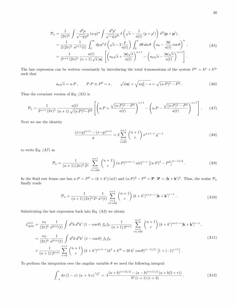
20
Pn =1
(2π)6
∫d3p√−g p0
(u·p)n∫
d3p′√−g p′0
δ
(√s− 1
a(t)(p+ p′)
)δ3(p + p′) ,
=1
2 (2π)51
an+1(t)
∫ ∞0
dp pnδ
(√s− 2
p
a(t)
) ∫ π
0
dθ sin θ
(u0 −
|u|a(t)
cos θ
)n,
=1
2n+1 (2π)5a(t)
(n+ 1)√s |u|
[(u0√s+|u|√s
a(t)
)n+1
−(u0√s− |u|
√s
a(t)
)n+1].
(A5)
The last expression can be written covariantly by introducing the total 4-momentum of the system Pµ = kµ + k′µ
such that
u0√s = u·P , P ·P ≡ P 2 = s ,
√s|u| =
√su20 − s =
√(u·P )2 − P 2 . (A6)
Thus the covariant version of Eq. (A5) is
Pn =1
2n+1 (2π)5a(t)
(n+ 1)√
(u·P )2−P 2
(u·P +
√(u·P )2 − P 2
a(t)
)n+1
−
(u·P −
√(u·P )2 − P 2
a(t)
)n+1 , (A7)
Next we use the identity
(x+y)n+1 − (x−y)n+1
y= 2
n+1∑r=1rodd
(n+ 1
r
)xn+1−r yr−1 (A8)
to write Eq. (A7) as
Pn =1
(n+ 1) (2π)5 2n
n+1∑r=1r∈ odd
(n+ 1
r
)(u·P )n+1−r a(t)1−r
[(u·P )2 − P 2
](r−1)/2. (A9)
In the fluid rest frame one has u·P = P 0 = (k + k′)/a(t) and (u·P )2 − P 2 = P ·P = (k + k′)2. Thus, the scalar Pnfinally reads
Pn =1
(n+ 1) (2π)5 2n1
an(t)
n+1∑r=1r∈ odd
(n+ 1
r
)(k + k′)n+1−r |k + k′|r−1 . (A10)
Substituting the last expression back into Eq. (A3) we obtain
C(n)gain =σT
(2π)61
a6+n(t)
∫d3k d3k′ (1− cos θ) fkfk′
1
(n+ 1) 2n+1
n+1∑r=1r∈ odd
(n+ 1
r
)(k + k′)n+1−r|k + k′|r−1 ,
=σT
(2π)61
a6+n(t)
∫d3k d3k′ (1− cos θ) fkfk′
× 1
(n+ 1) 2n+1
n+1∑r=0
(n+ 1
r
)(k + k′)n+1−r(k2 + k′2 + 2k k′ cos θ)(r−1)/2
[1 + (−1)r+1
].
(A11)
To perform the integration over the angular variable θ we need the following integral:∫ 1
−1dx (1− x) (a + b x)
r−12 = 4
(a+ b)(r+3)/2 − (a− b)(r+1)/2 (a+ b(2 + r))
b2 (r + 1) (r + 3), (A12)
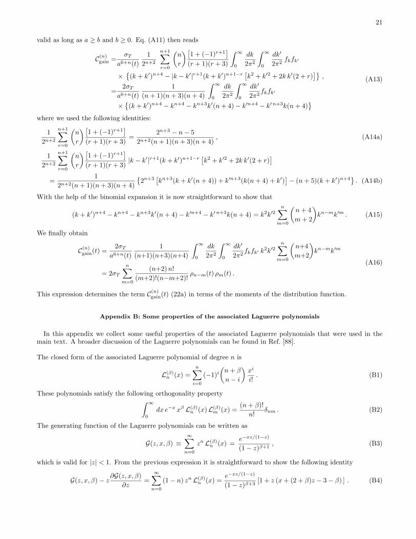
21
valid as long as a ≥ b and b ≥ 0. Eq. (A11) then reads
C(n)gain =σT
a6+n(t)
1
2n+2
n+1∑r=0
(n
r
)[1 + (−1)r+1
](r + 1)(r + 3)
∫ ∞0
dk
2π2
∫ ∞0
dk′
2π2fkfk′
×
(k + k′)n+4 − |k − k′|r+1(k + k′)n+1−r [k2 + k′2 + 2k k′(2 + r)]
,
=2σT
a6+n(t)
1
(n+ 1)(n+ 3)(n+ 4)
∫ ∞0
dk
2π2
∫ ∞0
dk′
2π2fkfk′
×
(k + k′)n+4 − kn+4 − kn+3k′(n+ 4)− k′n+4 − k′n+3k(n+ 4)
(A13)
where we used the following identities:
1
2n+2
n+1∑r=0
(n
r
)[1 + (−1)r+1
](r + 1)(r + 3)
=2n+3 − n− 5
2n+2(n+ 1)(n+ 3)(n+ 4), (A14a)
1
2n+2
n+1∑r=0
(n
r
)[1 + (−1)r+1
](r + 1)(r + 3)
|k − k′|r+1(k + k′)n+1−r [k2 + k′2 + 2k k′(2 + r)]
=1
2n+2(n+ 1)(n+ 3)(n+ 4)
2n+3
[kn+3(k + k′(n+ 4)) + k′n+3(k(n+ 4) + k′)
]− (n+ 5)(k + k′)n+4
. (A14b)
With the help of the binomial expansion it is now straightforward to show that
(k + k′)n+4 − kn+4 − kn+3k′(n+ 4)− k′n+4 − k′n+3k(n+ 4) = k2k′2n∑
m=0
(n+ 4
m+ 2
)kn−mk′m . (A15)
We finally obtain
C(n)gain(t) =2σT
a6+n(t)
1
(n+1)(n+3)(n+4)
∫ ∞0
dk
2π2
∫ ∞0
dk′
2π2fkfk′ k
2k′2n∑
m=0
(n+4
m+2
)kn−mk′m
= 2σT
n∑m=0
(n+2)n!
(m+2)!(n−m+2)!ρn−m(t) ρm(t) .
(A16)
This expression determines the term C(n)gain(t) (22a) in terms of the moments of the distribution function.
Appendix B: Some properties of the associated Laguerre polynomials
In this appendix we collect some useful properties of the associated Laguerre polynomials that were used in themain text. A broader discussion of the Laguerre polynomials can be found in Ref. [88].
The closed form of the associated Laguerre polynomial of degree n is
L(β)n (x) =
n∑i=0
(−1)i(n+ β
n− i
)xi
i!. (B1)
These polynomials satisfy the following orthogonality property∫ ∞0
dx e−x xβ L(β)n (x)L(β)
m (x) =(n+ β)!
n!δnm . (B2)
The generating function of the Laguerre polynomials can be written as
G(z, x, β) ≡∞∑n=0
zn L(β)n (x) =
e−xz/(1−z)
(1− z)β+1, (B3)
which is valid for |z| < 1. From the previous expression it is straightforward to show the following identity
G(z, x, β)− z ∂G(z, x, β)
∂z=
∞∑n=0
(1− n) zn L(β)n (x) =
e−xz/(1−z)
(1− z)β+3[1 + z (x+ (2 + β)z − 3− β) ] . (B4)
22
Appendix C: Derivation of Eq. (36)
In this appendix we present the details of the derivation of the Laguerre moments cn (36). From their definition (33)we can find their evolution by taking the derivative respect to τ
n∑r=0
(−1)r(n
r
)∂τMr =
n∑r=0
(−1)r(n
r
)[−Mr +
1
r+1
r∑m=0
Mm(τ )Mr−m
], (C1)
where we used explicitly the equation for the normalized moments (28). The last expression can be rewritten as
∂τ cn + cn =
n∑r=0
(−1)r(n
r
) [1
r+1
r∑m=0
MmMr−m
]. (C2)
Now all that remains to be proven is that the RHS of the previous expression corresponds exactly to the RHSof the Laguerre moment equation (36). In order to see the equivalence we substitute the definition of the Laguerremoments (33) on the RHS of Eq. (36):
1
n+ 1
n∑r=0
cr cn−r =1
n+ 1
n∑r=0
[r∑s=0
(−1)s(r
s
)Ms
] [n−r∑t=0
(−1)t(n−rt
)Mt
],
=1
n+ 1
n∑s=0
n∑t=0
(−1)t+sMsMt
[n∑r=0
(r
s
)(n−rt
)],
=
n∑s=0
n∑t=0
(−1)t+sn!
(s+t+1)! (n−s−t)!MsMt =
n∑q=0
(−1)q(n
q
) [1
q + 1
q∑s=0
MsMq−s
].
(C3)
This shows that the RHS of Eqs. (C2) and (C3) agree, and thus that the equation for the Laguerre moments (36)holds for any value of n ≥ 2. In Eq. (C3) we used the fact that
(nk
)= 0 if k > n and the combinatorial identity
n∑r=0
(r
s
)(n− rt
)=
(n+ 1
s+ t+ 1
)(C4)
which is valid if s, t ≥ 0 and s+ t ≤ n.
[1] C. Cercignani, R. Illner, and M. Pulvirenti, The Math-ematical Theory of Dilute Gases (Springer-Verlag, NewYork, (1994)).
[2] C. Cercignani, The Boltzmann Equation and Its Applica-tions (Springer-Verlag, New York, (1988)).
[3] A. V. Bobylev, Sov. Phys. Dokl. 20, 820 (1976).[4] M. Krook and T. T. Wu, Phys. Rev. Lett. 36, 1107
(1976).[5] M. Krook and T. T. Wu, Physics of Fluids 20, 1589
(1977).[6] S. Jeon and L. G. Yaffe, Phys. Rev. D53, 5799 (1996),
hep-ph/9512263.[7] J.-P. Blaizot and E. Iancu, Phys. Rept. 359, 355 (2002),
hep-ph/0101103.[8] J. I. Kapusta and C. Gale, Finite temperature field theory
Principles and applications (Cambridge University Press(New York), 2006).
[9] M. Le Bellac, Thermal Field Theory (Cambridge Univer-sity Press (New York), 1996).
[10] D. F. Litim and C. Manuel, Phys. Rept. 364, 451 (2002),
hep-ph/0110104.[11] D. F. Litim and C. Manuel, Nucl. Phys. B562, 237
(1999), hep-ph/9906210.[12] J.-P. Blaizot and E. Iancu, Nucl. Phys. B557, 183 (1999),
hep-ph/9903389.[13] V. Mathieu, A. H. Mueller, and D. N. Triantafyllopoulos,
Eur. Phys. J. C74, 2873 (2014), 1403.1184.[14] S. Jeon, Phys. Rev. C72, 014907 (2005), hep-
ph/0412121.[15] T. Epelbaum, F. Gelis, N. Tanji, and B. Wu, Phys. Rev.
D90, 125032 (2014), 1409.0701.[16] U. Heinz, Annals Phys. 168, 148 (1986).[17] U. Heinz, Phys. Rev. Lett. 51, 351 (1983).[18] H.-T. Elze and U. Heinz, Phys. Rept. 183, 81 (1989).[19] A. H. Mueller and D. T. Son, Phys. Lett. B582, 279
(2004), hep-ph/0212198.[20] F. Gelis, S. Jeon, and R. Venugopalan, Nucl. Phys.
A817, 61 (2009), 0706.3775.[21] S. A. Bass et al., Prog. Part. Nucl. Phys. 41, 255 (1998).[22] D. Molnar and M. Gyulassy, Nucl. Phys. A697, 495

23
(2002), [Erratum: Nucl. Phys.A703,893(2002)].[23] Z. Xu and C. Greiner, Phys. Rev. C71, 064901 (2005).[24] T. Epelbaum, F. Gelis, S. Jeon, G. Moore, and B. Wu,
JHEP 09, 117 (2015), 1506.05580.[25] S. Weinberg, Gravitation and Cosmology: Principles and
Applications of the General Theory of Relativity (JohnWiley & Sons, 1972).
[26] S. Weinberg, Cosmology (Oxford University Press, 2008).[27] C. Cercignani and G. Medeiros Kremer, The rela-
tivistic Boltzmann Equation: Theory and Applications(Birkhauser Verlag (Basel, Switzerland), 2002).
[28] J. Bernstein, Kinetic Theory in the Expanding Universe(Cambridge University Press, 1988).
[29] S. R. de Groot, W. A. van Leewen, and C. G. van Weert,Relativistic Kinetic Theory: principles and applications(Elsevier North-Holland, 1980).
[30] S. Dodelson, Modern Cosmology (Academic Press, 2003).[31] C.-P. Ma and E. Bertschinger, Astrophys. J. 455, 7
(1995).[32] M. Liebendoerfer, M. Rampp, H. T. Janka, and A. Mez-
zacappa, Astrophys. J. 620, 840 (2005).[33] H.-T. Janka, K. Langanke, A. Marek, G. Martinez-
Pinedo, and B. Mueller, Phys. Rept. 442, 38 (2007).[34] I. M. Oldengott, C. Rampf, and Y. Y. Y. Wong, JCAP
1504, 016 (2015).[35] G. Baym, Phys. Lett. B138, 18 (1984).[36] G. S. Denicol, U. Heinz, M. Martinez, J. Noronha, and
M. Strickland, Phys. Rev. D90, 125026 (2014).[37] G. S. Denicol, U. Heinz, M. Martinez, J. Noronha, and
M. Strickland, Phys. Rev. Lett. 113, 202301 (2014).[38] J. Noronha and G. S. Denicol, Phys. Rev. D92, 114032
(2015), 1502.05892.[39] Y. Hatta, M. Martinez, and B.-W. Xiao, Phys. Rev. D91,
085024 (2015).[40] M. Nopoush, R. Ryblewski, and M. Strickland, Phys.
Rev. D91, 045007 (2015).[41] G. Welke, R. Malfliet, C. Gregoire, M. Prakash, and
E. Suraud, Phys. Rev. C40, 2611 (1989).[42] W. Florkowski, R. Ryblewski, and M. Strickland, Phys.
Rev. C88, 024903 (2013), 1305.7234.[43] H. Marrochio, J. Noronha, G. S. Denicol, M. Luzum,
S. Jeon, and C. Gale, Phys. Rev. C91, 014903 (2015),1307.6130.
[44] J. Berges, A. Rothkopf, and J. Schmidt, Phys. Rev. Lett.101, 041603 (2008).
[45] K. Dusling, T. Epelbaum, F. Gelis, and R. Venugopalan,Nucl. Phys. A850, 69 (2011), 1009.4363.
[46] G. S. Denicol, H. Niemi, E. Molnar, and D. H. Rischke,Phys. Rev. D85, 114047 (2012), [Erratum: Phys. Rev.D91, 039902(E) (2015)].
[47] J. Berges, K. Boguslavski, S. Schlichting, and R. Venu-gopalan, Phys. Rev. D89, 074011 (2014), 1303.5650.
[48] J. Berges, K. Boguslavski, S. Schlichting, and R. Venu-gopalan, Phys. Rev. D89, 114007 (2014), 1311.3005.
[49] J. Berges, K. Boguslavski, S. Schlichting, and R. Venu-gopalan, JHEP 05, 054 (2014), 1312.5216.
[50] T. Epelbaum and F. Gelis, Phys. Rev. Lett. 111, 232301(2013), 1307.2214.
[51] E. Molnar, H. Niemi, G. S. Denicol, and D. H. Rischke,Phys. Rev. D89, 074010 (2014).
[52] A. Kurkela and E. Lu, Phys. Rev. Lett. 113, 182301(2014), 1405.6318.
[53] J. Berges, K. Boguslavski, S. Schlichting, and R. Venu-gopalan, Phys. Rev. Lett. 114, 061601 (2015).
[54] A. Kurkela and Y. Zhu, Phys. Rev. Lett. 115, 182301(2015), 1506.06647.
[55] J. Berges, K. Boguslavski, S. Schlichting, and R. Venu-gopalan, Phys. Rev. D92, 096006 (2015), 1508.03073.
[56] D. Polarski and A. A. Starobinsky, Class. Quant. Grav.13, 377 (1996), gr-qc/9504030.
[57] S. Yu. Khlebnikov and I. I. Tkachev, Phys. Rev. Lett.77, 219 (1996), hep-ph/9603378.
[58] T. Prokopec and T. G. Roos, Phys. Rev. D55, 3768(1997), hep-ph/9610400.
[59] D. T. Son, Phys. Rev. D54, 3745 (1996), hep-ph/9604340.
[60] D. T. Son (1996), hep-ph/9601377.[61] R. Micha and I. I. Tkachev, Phys. Rev. Lett. 90, 121301
(2003).[62] R. Micha and I. I. Tkachev, Phys. Rev. D70, 043538
(2004), hep-ph/0403101.[63] A. V. Frolov, JCAP 0811, 009 (2008), 0809.4904.[64] R. Allahverdi, R. Brandenberger, F.-Y. Cyr-Racine, and
A. Mazumdar, Ann. Rev. Nucl. Part. Sci. 60, 27 (2010),1001.2600.
[65] D. Bazow, G. S. Denicol, U. Heinz, M. Martinez,and J. Noronha, Phys. Rev. Lett. 116, 022301 (2016),1507.07834.
[66] H. Lee, Journal of Differential Equations 255, 4267(2013).
[67] H. Lee and A. D. Rendall (2013), 1301.0106.[68] D. Baumann, Cosmology Part III: Mathematical Tripos,
available at http://www.damtp.cam.ac.uk/user/db275/Cosmology/Lectures.pdf .
[69] F. Debbasch and W. van Leeuwen, Physica A: StatisticalMechanics and its Applications 388, 1079 (2009).
[70] F. Debbasch and W. van Leeuwen, Physica A: StatisticalMechanics and its Applications 388, 1818 (2009).
[71] S. Weinberg, Astrophys. J. 168, 175 (1971).[72] M. E. Peskin and D. V. Schroeder, An Introduction to
quantum field theory (Addison-Wesley (USA), 1995).[73] M. H. Ernst, Phys. Rep. 78, 1 (1981).[74] H. Grad, Commun. Pure Appl. Math. 2, 331 (1949).[75] W. Israel and J. M. Stewart, Annals Phys. 118, 341
(1979).[76] A. Muronga, Phys. Rev. C76, 014910 (2007).[77] J. Riordan, Combinatorial Identities (John Wiley &
Sons, New York, (1968)).[78] H. Cornille and A. Gervois, Journal of Statistical Physics
23, 167 (1980).[79] P. L. Bhatnagar, E. P. Gross, and M. Krook, Physical
Review 94, 511 (1954).[80] J. Anderson and H. Witting, Physica 74, 466 (1974).[81] P. B. Arnold, C. Dogan, and G. D. Moore, Phys. Rev.
D74, 085021 (2006), hep-ph/0608012.[82] G. S. Denicol, J. Noronha, H. Niemi, and D. H. Rischke,
Phys. Rev. D83, 074019 (2011), 1102.4780.[83] R. Baier, A. H. Mueller, D. Schiff, and D. T. Son, Phys.
Lett. B502, 51 (2001), hep-ph/0009237.[84] S. S. Gubser, Phys. Rev. D82, 085027 (2010).[85] U. Heinz and M. Martinez, Nucl. Phys. A943, 26 (2015).[86] J. D. Bjorken, Phys. Rev. D27, 140 (1983).[87] A. Krasinski, Inhomogeneous Cosmological Models
(Cambridge University Press, 1997).[88] G. B. Arfken, H. J. Weber, and F. E. Harris, Mathemat-
ical Methods for Physicists (Seventh Edition) (AcademicPress, Boston, 2013), seventh edition ed.