i

ii

EXECUTIVE SUMMARY The coastline of Chennai with a hinterland of 20km offer a variety of

environmental issues and problems, which need integrated management. These include

the coastal erosion and accretion, pollution from human settlement and industries, loss

of aesthetics in tourism beaches and declining fishery resources. The ICMAM Project

Directorate undertook the task of analysing above problems and prepared integrated

management solutions, which will help to solve these problems and also avoidance of

occurrence of such problems in future.

It is well known that the shoreline along Chennai coast is subjected to oscillations

due to natural and man made activities. After construction of Chennai port, coast north of

port is eroded and 350 hectares land is lost into sea. The river Cooum that carries

domestic sewage is closed due to accretion of sand south port. State Government

resorted to short term measures for protecting coastal stretch of length 6 km at

Royapuram with sea wall and the erosion problem shifted to further north. Now with the

construction of Ennore port, 16 km North of Chennai port, another erosion problem was

emerged and similar issues like Chennai port are on the way. If, no intervention is

planned, threat to ecologically sensitive Pulicat Lake is inevitable. North Ennore Coast is

already experiencing increased wave action and the naturally formed protection barriers,

the “Ennore Shoals”, may likely to be disturbed by construction of Port. Baseline data

reveal that the Ennore creek on south of Ennore port is experiencing increased siltation.

Since the available information on Ennore coast is not sufficient for working out

suitable measures, a research project entitled “Shoreline management along Ennore”

has been formulated to conduct detailed field and model investigations on various

dynamical aspects (water level variations, currents & circulation, tides, waves,

bathymetric variations, sediment transport, shoreline changes etc) of Ennore coast

covering Ennore creek to Pulicat mouth. The objective of the project is to develop

hindcast, nowcast and forecast models on shoreline changes in priority areas for

identification of vulnerable areas of erosion/ accretion to arrive at remedial measures for

protection of coastline from natural and human perturbations. The strategy proposed in

the present study aims at obtaining a comprehensive picture on shoreline changes along

Ennore coast and to take remedial measures for shoreline management along the

stretch.

iii

Coastal processes responsible for shoreline changes were monitored in

4 phases during the period 2004-2006. Field measurements on winds, waves, tides,

currents, sediments, beach profiles, bathymetry etc were conducted at selected

locations between Pulicat and Ennore creek. Seasonal variations on water levels, wave

climate, currents and circulation, sediment transport, shoreline changes etc were

studied. The measurements indicate that the tide propagates from south to north and

variation of tide range along the coast is insignificant. Currents are seasonal, northerly

during SW monsoon and southerly during NE monsoon. Wave climate indicate that 90%

of the waves approach the coast from SE direction and the remaining 10% from NE

direction. Sediment characteristics monitored at Ennore shoals indicate that the coarse

sediment occupied along the offshore boundary of the shoal and finer sediments

adjacent to the coastline. This aspect clearly demonstrates that the shoals while

interacting with large waves, reduces the energy of the incoming waves which results in

deposition of coarser sediment along the offshore boundary of the shoals. Finer

fragments of the sediment are carried over the shoal by relatively low energy waves and

deposit adjacent to the coastline. The simultaneous wave observations at shoals

indicate the wave energy is attenuated when they travel over shoals and the adjacent

coast is naturally protected by shoals. Beach profiles and shoreline positions were

monitored for two years for the coastal stretch between Pulicat and Ennore creek. The

observations at Pulicat indicated complete closure of bar mouth due to failure of

monsoon in recent years. The immediate 1 km length of coastal stretch abutting south

breakwater (updrift coast) accreted at a rate of 45 m per year, a 300 m wide beach

formed at south breakwater. The zone of accretion extended south upto 2.6 km that

eventually lead to rapid silting of Ennore Creek used to draw cooling water by power

plants mentioned earlier. North of Port, the coastline (beach fill area) eroded at 50 m per

year upto 1 km from the north breakwater and showed accretion thereafter due to

material originating from the fill region. After 2003, the coastline beyond nourishment

area (3 km) near Kattupalli village underwent readjustment that resulted in moderate

erosion of the order of 50 m.

Keeping in view of processes identified from filed investigations, model

investigations on hydrodynamical aspects, nearshore wave transformation processes,

sediment transport pattern and shoreline changes have been carried out. The models

are calibrated with the field data collected during the four phases of project work. By

iv

integrating the results of field and model investigations, the sediment budget for Ennore

coast was estimated. The existing sediment transport rates of the coast were also

determined. The areas prone to erosion and deposition (hot spots) have been identified.

Possible interventions for protection of Erosional hot spot located just immediate 1.5 km

north of Ennore port were tested for preparation of shoreline management plan.

Earlier, by anticipating erosion on north coast, the Ennore port authorities have

adopted the soft shore protection measure the “beachfill”, over a length of 4 km and

width 500 m. The present study indicated that the measure taken by port authorities

worked well. Modelling studies indicate that beach fill with a length of 1000 m plus

transitional length of 800m and width 600 m, resulted in increase in the life of the project

by one more year.

As a part of the study, the functional performance of the hard protection

measures like groins were tested through model simulations. Adoption of these options

helps to prevent erosion along the stretch under consideration, but the erosion problem

may likely to be shifted further north as there is no adequate sediment supply available

to north of Ennore Port due to trapping of sediments in the entrance channel.

Finally, the submerged reefs with sand bypassing seems to be a good option for

protection of Ennore coast since it not only reduced the wave energy but also provides

wave rotation which reduces convergence of energy on lee side of the reef. There may

not be a problem of shifting in erosion zone, that too, the option is more environmental

friendly. The present study recommends fabrication of submerged reefs with periodical

renewal as a long term solution to deal with the present and future problem of erosion on

north of Ennore coast. It is also strongly suggested that immediate initiation of such

remedial measures will help in non-repentance of delayed response leading to large loss

of land as occurred along the Royapuram coast of Chennai. The detailed structural

design of finalized option needs to be taken up, as it is not included under the present

scope of study.

v

Acknowledgements

We are thankful to the support extended by Ennore Port Authorities in terms of

utilizing their facilities for operation of survey vessels and the Public Works Department,

chennai for providing crest of berm data for the present work.

Contents

1 INTRODUCTION 2

1.1. Coastal Protection Measures – Experiences from other countries 3

1.2. Status of coastal Protection Measures along the Chennai and its relevance to study area

4

1.3. Brief description of the Project 10

1.4. Objectives 13

1.5. Project components/ tasks 13

1.6. Participating Institutions and their responsibilities 16

1.7. Present report 16

2 FIELD INVESTIGATIONS 29

2.1. Sea bed morphology/ Bathymetry 29

2.2. Winds 32

2.3. Waves 34

2.4. Tides 35

2.5. Currents and circulation 44

2.6. Suspended sediment distribution 59

2.7. Beach and Bedload sediment distribution 61

2.8. Littoral Environmental Observations 66

2.9. Beach profile changes 73

2.10. Shoreline changes 81

3 MODELLING 89

3.1. Hydrodynamic model 89

3.2. Wave model 94

3.3. Sediment transport model 104

3.4. Shoreline model 110

4 INTERVENTIONS 117

4.1. Artificial beach nourishment 118

4.2. Sand Nourishment 121

4.3. Groins 122

4.4. Offshore submerged reefs 131

5 RECOMMENDATIONS 152

REFERENCES 155

2

1. INTRODUCTION

Environmentally friendly solutions that are compatible with ever-changing needs of

the society are major challenges in coastal zone management today. Political, social and

technical issues must be considered, and possible solutions must balance the likely positive

and negative impacts. For centuries, the coastline has been a focus for a variety of activities

including industry, agriculture, recreation and fisheries. These national economic assets

have been developed and flourished despite constant changes in the physical characteristics

of the coast. The coastline is a national heritage and in order to sustain it for future

generations, proper management of coastal zone is essential. 'Coastal defence' means

protecting the coastline from erosion by the sea and defending low lying ground from

flooding by the sea.

Traditionally, coast and flood protection works have been implemented in a

piecemeal fashion, either in response to a recognized threat to an existing village or town, or

as part of a new development scheme. The authorities responsible for coastal defence and

flood protection tend to look at the issue within their own boundaries. The measures taken in

response to a problem, sometimes lead, often unintentionally, to adverse effects on both

adjoining and distant stretches of coastline.

Therefore, there is need for a well-defined plan that seek to treat the shoreline and

the defence requirements in a more integrated, sustainable and strategic manner. This can

be achieved by Shoreline Management Plan (SMP), which considers the issues at a

reasonable scale. The policy adopted should ensure adequate protection against flooding

and erosion in a manner that is technically, environmentally and economically acceptable,

both at the time any associated measures are implemented, and in the future.

For preparation of SMP, the boundaries of the region have to be identified properly to

avoid adverse impacts, arising from the interventions planned as a part of the Plan. The

processes along the shoreline vary spatially and temporarily. The inputs and outputs of the

region have to be assessed carefully depending on underlying processes. There are few

questions which still need to be answered by scientific experiments. They are

i) The coastal stretch considered is dominated by onshore - offshore transport

or along shore transport

3

ii) The magnitude of the sediment transport in onshore, offshore and along

shore

iii) The modification of sediment pathways along the coastal stretch resulting

from man made interventions. These include construction of dams on upstream of the river,

major harbour installation along the coast, sand mining etc.

1.1 Coastal Protection Measures - Experiences from other countries

The mitigation measures implemented along the coastal areas in Europe and

USA clearly indicate that the functional performance of the measures could not be met

due to lack of understanding of underlying of coastal processes, as it requires

continuous monitoring of various parameters (tides, waves, currents, sediment

transport etc.). The key environmental and structural parameters governing shoreline

response to structures are yet to be elucidated. Before engineering design guidelines

can be developed for coastal protection structures, a fundamental research challenge

is to establish the mechanisms that cause erosion or accretion in their lee or adjacent

to the structure. The experiences from the few cases where structures (Groins,

Offshore breakwater) built for the coastal protection are briefed below:

The groins are built to stabilize a beach, where erosion is generated by a net

longshore loss of sand. Groins are most effective where the longshore transport has a

strong predominant direction and where this action will not create unacceptable

downdrift erosion (USACE, 2001). A well-designed groin field will fill and allow natural

sand bypassing at nearly pre-groin conditions, thus reducing downdrift erosion.

Nonetheless, groin projects have met with varied success in part because of vague

definitions of functional design criteria (CERC, 1984). With few exceptions, functional

design criteria are defined in relative terms. Furthermore, earlier design practices were

limited because ascertaining proper functional design was usually an exercise in trial-

and-error. However, recent advances in numerical computer simulation can be used to

approximate performance and shoreline behaviour in response to discrete groin design

characteristics (USACE, 1995), for which information on coastal processes and

shoreline changes is required.

Functional design criteria refer to those critical design factors that must be

considered in order for a groin system to offer an acceptable solution to a discrete

erosion problem; yet not instigate accelerated erosion along adjacent beaches

(USACE, 1995). According to BALSILLIE and BERG, (1972) there are three groin

4

design considerations; i) littoral processes (wind and wave data, beach slope, sediment

type etc.); ii) functional design criteria (length, height, spacing etc.); and iii) structural

design criteria (material types, construction procedures etc.). Among the three design

considerations, the first part was addressed completely as part of this project and

second aspect which deals with dimensions of the structure was partially dealt.

Structural design was not addressed in the present scope of the project.

Shoreline response to the structures along different parts of the world was

reviewed by Turner (1994) in terms of its functional performance. Six such cases were

reviewed based on the field monitoring studies conducted at respective places. The

objective of this review is to assess the critical parameters for design of coastal

structures. Of the reported parameters of breakwater length, crest submergence level,

crest width, nearshore slope, littoral drift rates, and the presence or absence of

concurrent sand nourishment, none appears to be critical in governing shoreline

response characteristics of submerged breakwaters. It may be specific combinations

of these parameters that are important, but it is reported that additional design and

environmental factors must be considered.

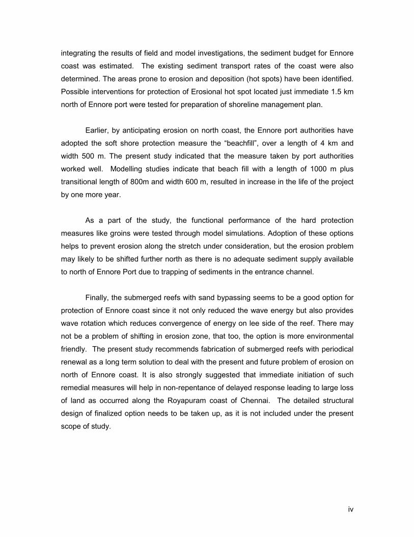
1.2 Status of coastal protection measures along the Chennai and its relevance to study area Sediment inputs to the Ennore coast depends on the geomorphology of the coast

and man-made interventions made on adjacent coast. The status of coast, south of

Ennore creek to Adayar river (Fig. 1.1) was studied for shoreline changes. The 11 km in

length of the coast extending from fishing harbour to Ennore creek is under enormous

stress due to an increased industrial growth combined with harbour facilities, resulted

changes in coastal dynamics. The rate of sediment transport (Chandramohan et al.

1990) is towards the north from March to October and towards the south from November

to February. The net drift towards north is in the order of 0.3 x 106 m3 per year. Ever since

the Chennai harbour was constructed, the coast north of the harbour has been

experiencing erosion at the rate of about 8 meters per year. It is estimated that 500

meters of beach has been lost between 1876 and 1975 and another 200 meters between

1978 and 1995. History reveals that in the year 1876 a jetty projecting into the sea was

constructed at Chennai for unloading of the cargo. Later, breakwaters were constructed

on either side of the jetty (with the harbour entrance located on the eastern side), to

protect the facility from wave disturbance, without realizing the effect of east entrance on

5

tranquility in the harbour basin. Subsequently, the entrance to the harbour was shifted to

the north and the harbour expanded further parallel to the coast for operational reasons.

Schematic diagram (Fig. 1.1) shows the present day configuration of the Chennai port

and the growth of the beach on the southern side over the years. Marina Beach has been

formed as a result of arresting the littoral drift by the breakwater. The north Chennai

coast, extending from the fisheries harbour is fragile and is very sensitive for change in

the environmental conditions. One of the main reasons for this delicate response of the

coastal stretch is the disruption in sediment supply induced by the Chennai port causing

extensive erosion over the years. This has been aggravated by the rough sea conditions

during the northeast monsoon. Wave overtopping and undermining of the coast due to

unprecedented wave actually has caused substantial damage to the coastal region.

6

Fig. 1.1 - Present day configuration of Chennai coast

7

The consequences of the construction of Chennai port and Fishing harbour on the North

Chennai coast are detailed below.

The shoreline has recessed by about 1000 m with respect to the original shoreline in

1876. The villages, hutment and the Royapuram-Ennore express highway connecting the Manali

Refineries and Thermal Power Station to Chennai are subjected to sea erosion during both

Southwest and Northeast monsoons every year. The erosion in the coast which became very

pronounced, affected the coastline up to the 13/150 KM stone near Bharathi Nagar and

necessitated constant attention and protective works in response to the cry of the fishermen

living in this stretch.

In order to protect the coastline, the State authorities resorted to construction of short-

term protective structures. They have recommended the use of sand dredged at Chennai port to

nourish North Chennai-Royapuram as a long-term measure and construction of Rubble Mound

Stone wall and groins as short-term measures. Part of this protected coastal stretch experiences

undermining of the seabed due to large-scale wave action. The erosion along this coast has

reached an alarming stage requiring immediate attention (Kalisundram et. al, 1991). It is

estimated that an area of 260 hectares of land was lost between the years 1893 and 1955 and

that an area of about 30 hectares was destroyed by the wave action between the years 1980 and

1989. Overall loss between the period 1893 and 1989 is estimated to be of the order of 350

hectares. The cost of land alone, lost to the sea, is of the order of approx. Rs.200 crore (US $40

million). During and after 1990 this stretch of coastline was threatened by severe waves and the

authorities resorted to new techniques involving erection of concrete pipes to protect the

shoreline. However, this did not provide much of remedy and about 50m wide beach must have

been lost after 1990. Devastating effects due to the wave overtopping and severe erosion led to

the destruction of the coastal highway and compulsory rehabilitation of fishermen (about 200

families) to safer places. The shoreline receded by about 100 m between 1978 and 1995.

Though the short-term measures taken up by authorities gave temporary solution to the

villages in protected areas, the problem is not resolved completely. Due to the construction of

stone wall (Fig. 1.2), the natural beach available is lost and the downdrift villages, north of

protected areas started experiencing erosion. The village Chinnakuppam near Ennore fly ash

outfall is experiencing severe erosion.

8

Fig. 1.2 - Sea wall along Rayapuram Highway The figures of dredging quantities provided by the Dredging Corporation of India indicate

a variation between 0.27 million m3 and 1.10 m3. It has been reported that the annual

maintenance dredging at Chennai port is in the order of 0.5 million m3. This dredged material is

being dumped to the east of harbour, as dredgers are unable to reach nearer to the shore due to

shallow draft.

The short-term protection to the coastline by dumping stones is found to be ineffective for

the reasons that (i) the nearshore coastal processes in the region are not clearly understood, (ii)

inadequate funds usually restrict the required quantity of rubble for the protection and

maintenance, which make remedial measures as ineffective and (iii) lack of continuous

monitoring (Mani, J.S 2001).

The above case, clearly stressed the need for a shoreline comprehensive plan to manage

the multiple resources and uses of shorelines in a manner that is consistent with requirement

and purposes and addresses the needs of the public. The management plan should ensure a

9

balance that supports local economic interest, protect environmental resources and allows the

public to enjoy those resources and all these are vital for the long-term success of a Shoreline

Management Plan (SMP).

Similarly, due to the newly emerged Ennore satellite port, the north coast near Kattupalli

village is under severe erosion and the Ennore creek located 2.6 km south of port is experiencing

siltation. Ennore creek carries industrial effluents generated from adjoining land based activities.

The decreased flushing characteristics due to siltation leads to degradation of water quality and

causing major environmental problems and the Enore coast has become a hot spot in relation to

coastal zone management.

10

Fig. 1.3 – Chennai – Ennore coast

1.3 Brief Description of the project

The critical analysis of issues related to shoreline management along the chennai coast

reveals that the impacts are due to natural aspects, e.g. change in wave climate, failure of

monsoon and sediment depletion and man made activities viz., development of ports, coastal

structures and activities at upstream of estuaries. Measures attempted to protect the coast from

erosion and free from siltation could not give fruitful solutions due to lack of understanding of

11

coastal processes. Creation of another (Ennore) port in a region that is already highly sensitive

to sediment transport is bound to lead to further complexities in terms of coastal erosion and/or

accretion. At present, the southern coast of Ennore is witnessing accretion (attributable to

breakwater) and, a tidal creek some 2.6 km away is silting up rapidly causing concern to nearby

Power Plants drawing cooling water from it. Artificial beach nourishment (to prevent downdrift

erosion) was therefore taken up in the year 2000 by placing 3.5x106 m3 of sand dredged from the

harbour basin and the approach channel through capital dredging. Under these circumstances, a

careful assessment of shore protection measures for optimum performance and likely cross

impacts on adjacent coast would appear essential for any judicious implementation of coastal

zone management practices.

The coastal stretch considered for the study (Fig 1.3) is located in north Chennai coast

and is highly sensitive to the sediment transport. Ennore Port, constructed 16 km North of

Chennai port would also result in similar issues like Chennai port. If, no intervention is planned,

threat to ecologically sensitive Pulicat Lake is inevitable. North Chennai Coast is already

experiencing increased wave action and the naturally formed protection barriers “ Ennore

Shoals” may likely to be disturbed by construction of the Port. In view of this a research project

entitled “Shoreline management plan for Ennore coast” was formulated for a detailed study on

various coastal dynamical aspects. The objective of the project is to develop hindcast, nowcast

and forecast models on shoreline changes in priority areas for identification of vulnerable areas

of erosion/ accretion and to predict changes in the future to develop appropriate remedial

measures for protection of coastline from natural and human perturbations.

12

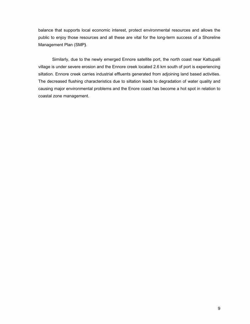
Fig. 1.4 – Study area and station locations

The study area comprises mainly 3 zones i.e. a) zone I – the 5km coastal stretch each on

North and South side of Ennore port including Ennore creek (Fig 1.4). b) Zone II – the coastal

stretch in between North Kattupalli and south Pulicat mouth which occupies mostly sand dunes

and c) Zone III – the 2km coastal stretch on North and South of Pulicat mouth which occupies a

narrow channel opening into the sea . The study area extends from shoreline to 25m depth

contour.

13

1.4. Objectives

� To identify the areas which are vulnerable to erosion/ accretion due to shoreline

changes caused by construction of Ennore port through field studies

� Identification of dominant forcing functions and evaluation of earlier preventive

measures.

� To develop hindcast and forecast models for prediction of shoreline changes using

the primary data

� Validate Numerical Models for field conditions to address issues in Nearshore -

Erosion & Siltation at Inlet

� To prepare a shoreline management plan suggesting measures for protection of the

coast from erosion / accretion

1.5. Project components/tasks

The study involved both field and model investigations. Major project components are

• Assessment of present status and detect shoreline changes at Ennore port by using

past data

• Identification of vulnerable areas for erosion/ accretion

• Monitoring of processes responsible for shoreline changes such as waves, tides,

currents, sediment characteristics, beach profiles and morphology, etc.

• Monitoring of Ennore shoals and its role in protection of North Chennai coast

• Development of Impact models and prediction of future changes using MIKE 21 &

LITPACK models

• Integration of results for mapping of vulnerable areas for erosion/accretion through

GIS

• Recommendations of Interventions like sand bypassing/ groins/ offshore breakwater/

submerged reefs for protecting the coast from erosion/accretion

The monitoring scheme for understanding the processes responsible for shoreline

changes covers two seasons i.e. NE monsoon (Phase I & III periods) and SW monsoon (Phase

II period) and measurements were made at 7 stations (Fig 1.5) that include measurements of

� Tides/water levels at 7 stations (D1 to D7) by deploying tide gauges in coastal waters

and harbour

14

� Current meter recording at 6 stations (D1 to D7 except at D4) - 3 in mooring and

3 from boat

� Wave measurements at 7 locations by pressure gauge and 6 months from NDBP

Buoy

� Littoral Environmental Observations (LEO) between Ennore and Pulicat (2 seasons)

� Measurement of current profiles along 3 transects using ADCP, ADP and ADV

� Weather data recording at Ennore Port by installing weather station

� Random water and sediment sampling at 34 stations (sts R1 to R34) for 3 phases

� Beach sediment sampling at upper and lower foreshore along the transects T1 to T7

(2 phases - NE and SW)

� Beach profile and bathymetric profile across the shore along each transects T1 to T7

(2 phases - NE and SW)

� Shoreline mapping between Ennore and Pulicat (quarterly during study period and

annually from 1999)

� Bathymetry for the year 2000 & 2005 (20 km coast)

15

Fig. 1.5 – Study area with zones

16

1.6. Participating Institutions and their responsibilities

ICMAM Project Directorate Responsibilities

Shri M. V. Ramana Murthy, Sci.E Co-ordination of project activities, project design; Organizing field campaigns and collection of field data

on hydrodynamics; Periodical review of field data and models and preparation of Shoreline Management Plan

Dr V. Ranga Rao, Sci.D Organizing field campaigns, beach profile survey,

analysis, first level modeling and preparation of report

Dr.Manjunath Bhat, RA Deployment/ retrieval of field equipment, bathymetry &

ADCP survey, analysis of data, shoreline change

modeling

Edwin Rajan, T.A Setting and operation of Instruments, deployment and

bathymetry survey

Y.Pary Vallal, SRF All GIS work related to mapping of shoreline changes, bathymetry & ADCP survey

M.Padmanabham, JRF Analysis of tide, current and ADP data

Dr. B.R. Subramanian, Sci,G and Advisor (Project Director)

Overall in-charge of the project, Project conception, review of draft Shoreline Management Plan

NIOT Responsibilities

Dr Rajat Roy Chaduary, Sci. F Overall logistic and administrative support for project activities

Dr B.K.Jena, Sci. D

Support in organizing field data collection, timely

support for logistics and deployment

Mr.Jaiprakash, T.A Assistance in deployment and survey

1.7. Present report

The present report deals with the entire work carried out (Table 1.1) during the four

phases i.e. Phase I (Nov/Dec 2004), Phase II (Apr/May 2005), Phase III (Dec 2005) and Phase

IV (Aug 06) of project duration. Secondary information on shoreline changes from PWD,

Chennai; weather data from IMD, Chennai were also collected and analyzed. All the field data

collected during the above four phases were processed and analyzed. Spatial as well as

temporal variations of various coastal oceanographic parameters and the features identified were

thoroughly discussed and presented.

The coastal process studies include the monitoring of hydrographic, sediment and

shoreline changes. The parameters monitored and type of instrumentation deployed and

analytical instruments used for data analysis, are detailed below:

17

Table 1.1 - Details of parameters monitored and instruments used

S No. Parameter Instrument No. of locations

1. Tides/waters inside the harbour and open coast

Directional and non-directional tide gauges, Valeport

7

2. Waves (directional/ non-directional)

Directional and non-directional tide gauges, Valeport

3

3. Coastal currents RCM 9 Current Meters, Aanderaa

6

4. Nearshore current profile Acoustic Doppler Profiler (ADP), Sontek

1

5. Wave orbital velocities and mean nearshore currents

Acoustic Doppler Velocimeter (ADV) with optical back scatter (OBS), Sontek

1

6. Bathymetry survey Echosounder, Odom and Heave Sensor, TSS

--

7. Bed sediments Mud Grab Samplers, Hydrobios

34

8. Suspended sediments Water Samplers, Niskin 34

9.

LEO observation (longshore current, brim height and surf zone width)

Floats

5

10. Beach profiles RTK GPS SR 530, Leica and Total Station, TPS 1100, Leica

20 km coastline at 500 m

transects 11. Shoreline mapping Arc Pad, GS 5+, Leica 20 km coastline

12. Meteorological parameters

Automatic Weather Station, R.M. Young

--

Laboratory Analysis S No. Parameter Instrument

1. Grain size distribution (coarser sediments)

Analytical Sieve Shaker( Retsch)

2. Particle size distribution (finer sediments)

Particle Size Analyser, Master Sizer 2000 ( Malvern)

The observations were made in 4 phases between November 2004 and August 2006.

The Wave and Tide Gauges were deployed in coastal waters to measure tides and waves

simultaneously. Currents were measured using automatic current meters at some of the

locations, where waves were measured. A typical mooring design adopted for simultaneous

monitoring of tides, currents and waves is shown in Fig 1.6. Acoustic Doppler Profiler (ADP)

and Acoustic Doppler Velocimeter (ADV) were deployed in nearshore between 0 m and 8 m

18

water depth at selected transects. At some locations, the data on tides and waves could not be

retrieved due to malfunctioning of the equipment (2 Nos.) and loss of the mooring (1 location)

due to rough weather condition inspite of several test checks conducted on functionality of

equipment.

Fig 1.6 a) - Mooring used for deployment of Wave and Tide gauge and current meter

19

Fig. 1.6 b) - Instruments used for Monitoring Nearshore parameters

It was proposed to collect wave data for 1 year using Directional Wave Rider Buoy, NIOT,

at a water depth of 23 m for assessing annual wave climate and for validation of numerical

model. But, due to vandalism and delay in redeployment, the data could be collected only for 6

months (Table 1.1) against intended plan of 1 year. Phase IV observations with three directional

wave gauges on north of port were undertaken to validate the numerical models and partially to

bridge the data gap in Directional Wave Rider Buoy data. Field experiments forms an essential

part for the ocean/ coastal processes and for validation of numerical models. Undertaking

oceanographic measurements is challenging task, requires enormous efforts in terms of

deployment, retrieval and maintenance of instruments during deployment period. Coastal

measurements along Indian coast are sparse and maintaining instruments at site is labour

intensive. Most of observations are discontinued prior to intended period due to logistic problems

and severe weather conditions. During the field experiment conducted at Ennore, enough care

20

was taken while collecting the coastal data in terms of deployment, maintaining the equipment

through watch and ward and retrieval. Details of deployment such as location, parameter,

measuring interval and duration of observations at each station for four phases of observation

are shown in Tables 1.2 - 1.5.

21

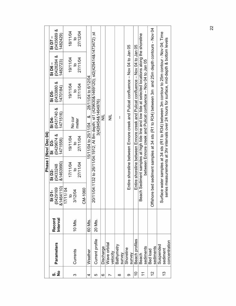
Table 1.2 – Details of data collection during phase I period (Nov/ Dec 04)

Phase I (Nov/ Dec 04)

S.

No

Parameters

Record

Interval

St D1-

(0429169

&1464110)

St D2-

(0433248

&1463990)

St D3-

(0429674 &

1471558)

St D4-

(0431740 &

1471516)

St D5-

(0433880 &

1470184)

St D6 –

(0428284 &

1482723)

St D7 –

(0435689 &

1482429)

1

Tides/water

level

Sampling

frequency

of 4 Hz for

60 sec

&

measuring

interval of

10 Min.

17/11/ 04

to

3/12/04

17/11/04

to

26/11/04

&

28/11/04

to

3/12/04

TG-19036

17/11/04

to

26/11/04

17/11/04

to

26/11/04

TG-19030

19/11/04

to

26/11/04

19/11/04

to

26/11/04

TG-21164

19/11/04

to

26/11/04

19/11/04

to

26/11/04

TG-21163

19/11/04

to

26/11/04

19/11/04

to

26/11/04

TG-21170

18/11/04

to

17/12/04

18/11/04

to

17/11/04

TG-21165

18/11/04

to

26/11/04

18/11/04

to

26/11/04

TG-19034

2

Waves

Sampling

frequency

of 4Hz with

1024

samples &

Measuring

interval of

60 Mts.

17/11/ 04

to

3/12/04

17/11/04

to

26/11/04

19/11/04

to

26/11/04

19/11/04

to

26/11/04

19/11/04

to

26/11/04

18/11/04

to

17/12/04

18/11/04

to

26/11/04

22

Phase I (Nov/ Dec 04)

S.

No

Parameters

Record

Interval

St D1-

(0429169

&1464110)

St D2-

(0433248

&1463990)

St D3-

(0429674 &

1471558)

St D4-

(0431740 &

1471516)

St D5-

(0433880 &

1470184)

St D6 –

(0428284 &

1482723)

St D7 –

(0435689 &

1482429)

3

Currents

10 Mts.

17/11/ 04

to

3/12/04

CM-1060

17/11/04

to

27/11/04

19/11/04

to

27/11/04

No cur

meter

19/11/04

to

27/11/04

19/11/04

to

27/11/04

18/11/04

to

27/12/04

4

Weather

60 Mts.

15/11/04 to 25/11/04 & 28/11/04 to 6/12/04

5

Current profile

20 Mts.

20/11/04:1132 to 26/11/04:1912; At 8m depth; st1 (429630&1469120); st2(429414&1473472) ;st

3(428454&1464976)

6

Discharge

NIL

7

Wave orbital

velocity

NIL

8

Bathym

etry

survey

--

9

Shoreline

survey

Entire shoreline between Ennore creek and Pulicat confluence – Nov 04 to Jan 05

10

Beach profiles

Entire shoreline between Ennore creek and Pulicat confluence – Nov 04 to Jan 05

11

Beach

sediments

Beach Sediment samples at high tide line and low tide at selected locations along the shoreline

between Ennore creek and Pulicat confluence – Nov 04 to Jan 05

12

Bed load

sediments

Offshore bed sediment samples at 34 sts (R1 to R34) between 3m and 25m depth contours - Nov 04

13

Suspended

sediment

concentration

Surface water samples at 34 sts (R1 to R34) between 3m contour to 25m contour - Nov 04; Time

series measurements at 3hr intervals over 24 hours for surface, mid-depth & bottom levels

23

Table 1.3 – Details of data collection during phase II period (Apr/May 05)

Phase II (Apr/ M

ay 05)

S.No

Parameters

Record

Interval

St D1-

(0429169

&1464110)

St D2-

(0433248

&1463990)

St D3-

(0429674 &

1471558)

St D4-

(0431740 &

1471516)

St D5-

(0433880 &

1470184)

St D6 –

(0428284 &

1482723)

St D7 –

(0435689 &

1482429)

1

Tides/water level

Sampling

frequency

of 4 Hz for

60 sec

&

measuring

interval of

10 Min.

30/3/05

to

30/4/05

30/11/05

to

30/4/05

Instrument

lost

31/3/05

to

18/4/05

31/3/05

to

17/4/05

Instrument

lost

31/3/05

to

20/4/05

31/3/05

to

20/4/05

31/3/05

to

30/4/05

31/3/05

to

30/04/05

31/3/05

to

8/5/05

31/3/05

to

8/5/05

2

Waves

Sampling

frequency

of 4Hz

with 1024

samples &

Measuring

interval of

60 Mts.

30/3/05

to

30/4/05

- do -

30/3/05

to

18/4/05

Instrument

error

31/3/05

to

20/4/05

31/3/35

to

30/4/05

31/3/05

to

8/5/05

3

Currents

10 Mts.

30/3/05

to

30/4/05

- do -

31/3/05

to

18/4/05

-do -

30/3/05

to

20/4/05

30/3/0

to

30/4/05

31/3/05

to

30/4/05

4

Weather

60 Mts.

25/4/05 to 6/5/05

5

ADP vertical

profiles

20 Mts.

6/4/05:1300 to 15/4/05:1700 (6mdepth (428960&1464783); 7m depth(43015&1469611); 8m

depth(429637&1473514 & 9m depth(426950 & 1488441)

6

ADCP discharge

nil

7

ADV orbital

velocities

6/4/05:1400 to 6/4/05:1500 5m depth(428735 & 1464960); 4m depth(429485&1469576); 5m

depth(426536&1488316) 6m depth (429379 & 1473486)

24

Phase II (Apr/ M

ay 05)

S.No

Parameters

Record

Interval

St D1-

(0429169

&1464110)

St D2-

(0433248

&1463990)

St D3-

(0429674 &

1471558)

St D4-

(0431740 &

1471516)

St D5-

(0433880 &

1470184)

St D6 –

(0428284 &

1482723)

St D7 –

(0435689 &

1482429)

8

Bathym

etry survey

Bathym

etric survey between 3 and 25m depth contours. Area covered between Ennore creek and

Pulicat mouth

9

Arcpad survey

Entire shoreline between Ennore creek and Pulicat confluence – Apr 05 to May 05

10

RTK beach profiles

Entire shoreline between Ennore creek and Pulicat confluence – Apr 05 to May 05

11

Beach sediment

Beach Sediment samples at high tide line and low tide at selected locations along the shoreline

between Ennore creek and Pulicat confluence – Apr 05 to May 05

12

Bed load sediment

Offshore bed sediment samles at 34 sts (R1 to R34) between 3m and 25m depth contours - Apr 05

13

Suspended

sediment

Surface water samples at 34 sts (R1 to R34) between 3m contour to 25m contour - Apr 05;

25

Table 1.4 – Details of data collection during phase III period (Dec 05/Jan 06)

Phase III (Dec 05/Jan06)

S.No

Parameters

Record

Interval

St D1-

(0429169

&1464110)

St D2-

(0433248

&1463990)

St D3-

(0429674 &

1471558)

St D4-

(0431740 &

1471516)

St D5-

(0433880 &

1470184)

St D6 –

(0428284 &

1482723)

St D7 –

(0435689 &

1482429)

1

Tides/water level

Sampling

frequency

of 4 Hz for

60 sec

&

measuring

interval of

10 Min.

17/1/06

to

7/2/06

nil

19/1/06

to

31/1/06

19/1/06

to

31/1/06

nil

20/1/06

to

26/1/06

nil

2

Waves

Sampling

frequency

of 4Hz

with 1024

samples &

Measuring

interval of

60 Mts.

17/1/06

to

7/2/06

nil

19/1/06

to

31/1/06

19/1/06

to

4/2/06

nil

20/1/06

to

27/1/06

nil

3

Currents

10 Mts.

17/1/06

to

14/2/06

CM-1110

nil

18/1/06

to

31/1/06

CM-664

19/1/06

to

31/1/06

CM-1120

nil

20/1/06

to

27/1/06

CM-1116

NIL

4

Weather

60 Mts.

Weather data monitored during 1/2/06 to Feb06

5

ADP vertical profile 20 Mts.

17/1/06:1716 TO 22/1/06:1056 AND 22/1/06:1144 to 8/1/06:1050

6

ADCP discharge

Cross-shore profiles at selected cross-section from Marina beach to Kalanji along ennore during 7-13

feb06

26

Phase III (Dec 05/Jan06)

S.No

Parameters

Record

Interval

St D1-

(0429169

&1464110)

St D2-

(0433248

&1463990)

St D3-

(0429674 &

1471558)

St D4-

(0431740 &

1471516)

St D5-

(0433880 &

1470184)

St D6 –

(0428284 &

1482723)

St D7 –

(0435689 &

1482429)

7

ADV orbital

velocities

23/1/06:1017 TO 23/1/06:1121 AND 18/1/06:1758 to 18/1/06:1902

8

Bathymetry survey

Bathym

etric survey between 3 and 25m depth contours. Area covered between Ennore creek and

Pulicat mouth

9

Arcpad survey

selected bathym

etry track were made along Ennore-pulicat coast jan06

10

RTK beach profiles

Entire shoreline between Ennore creek and Pulicat confluence – Jan-feb06

11

Beach sediment

Beach Sediment samples at high tide line and low tide at selected locations along the shoreline

between Ennore creek and Pulicat confluence – jan06-feb06

12

Bed load sediment

Offshore bed sediment samples at 34 sts (R1 to R34) between 3m and 25m depth contours – feb06

13

Suspended

sediment

Surface water samples at 34 sts (R1 to R34) between 3m contour to 25m contour – jan06

27

Table 1.5 – Details of data collection during phase IV period (Aug. 06)

Phase IV (Aug. 06)

S.No

Parameters

Record

Interval

St D3-(0429674 &

1471558)

St D4-(0431740 &

1471516)

St D5-(0433880 &

1470184)

1

Tides/water level

Sampling

frequency of

4 Hz for 60

sec

&

measuring

interval of

10 Min.

19/08/06

to

01/09/06

19/08/06

to

05/09/06

19/08/06

to

05/09/06

2

Waves

Sampling

frequency of

4Hz with

1024

samples &

Measuring

interval of

60 Mts.

19/08/06

to

01/09/06

19/08/06

to

05/09/06

19/08/06

to

05/09/06

3

Currents

10 Mts.

19/08/06

to

01/09/06

C-1116 & 1064

19/08/06

to

05/09/06

C-1064 & 1116

19/08/06

to

05/09/06

C-1059

4

ADP vertical profile

20 Mts.

09/08/06 to 25/08/06 (south of Ennore Port), 25/08/06 to 25/08/06 (at D3 location)

and 25/08/06 to 04/09/06 (D5 location)

5

ADCP discharge

26/08/06 offshore Kalanji

6

ADV orbital velocities

21/08/06 to 04/09/06 at 4 m depth off Kalanji

7

Bathymetry survey

Bathym

etric survey between 3 and 25m depth contours. Area covered between

Ennore creek and Pulicat mouth

28

8

Arcpad survey

selected bathym

etry track were made along Ennore to Kalanji (Aug. 06)

9

RTK beach profiles

Entire shoreline between Ennore creek and Kalanji – Aug. 06

10

Beach sediment

Beach Sediment samples at high tide line and low tide at selected locations along

the shoreline between Ennore creek and Kalanji – Aug. 06

11

Bed load sediment

Offshore bed sediment samples at 34 sts (R1 to R34) between 3m and 25m depth

contours – Aug. 06

12

Suspended sediment

Surface water samples at 34 sts (R1 to R34) between 3m contour to 25m contour –

Aug. 06

29

2. FIELD INVESTIGATIONS

2.1 Seabed Morphology/ Bathymetry

Seabed morphology of the Ennore region (Ennore creek to Pulicat) was mapped

using surveys conducted during May 2000 and April 2005. The bathymetry survey was

carried out for the area of 20-km on parallel (north to south) and 4km on perpendicular (east

to west) to the coast. The data was collected upto a water depth of 25m. Single beam

(ODAM) echosounder was used. The single beam echo sounder, (ODOM Hydrotrac, USA)

was fixed in the boat along with heave sensor and DGPS. Potential errors, such as vessel

roll, pitch, and yaw, and time lag between the positioning sensor (GPS) and the sonar

measurement, are recorded with on board instrumentation and incorporated into the post-

processing procedure (USACE, 2001). Care was taken to prevent/minimize other errors

such as inaccurate alignment of sensors, transducer draft depth, and sound velocity

measurements (USACE, 2001). The area to be surveyed was marked with grid spacing of

100 m on the background of satellites map (IRS 1D Pan) and the line position was

maintained by interfacing DGPS to PC based software (HYPACK 4.0). Since the coastal

environments display more variation in the cross-shore direction than the alongshore

direction the transect survey was performed perpendicular to the shoreline. Tidal corrections

have been applied to the data in post processing mode by using the simultaneously

recorded tide at Ennore and Pulicat. It is necessary to interpolate survey data in order to

produce a continuous bathymetric map. Hence the observed data was post processed,

analyzed and interpolated using HYPACK MAX survey software and the seabed elevation

with respect to chart datum was prepared using ArcGIS software.

30

Fig 2.1 – Bathymetry of Ennore coast

31

The seabed morphology at Ennore coast (Fig 2.1) is complex with varied slope

between Ennore creek and Pulicat lake. The slope at south of Ennore Port is relatively

steep (1 in 300) at Ennore creek, while the slope on northern side is flat (1 in 500) with

submerged shoals extending in northeasterly direction. It has been hypothesized that shoals

might have formed due to interaction of northerly coastal currents and sediment supply

through Ennore creek (Kosattalaiyar river) when it was active. The cross-sectional profiles

made at 1 km interval between Ennore creek and Pulicat lake (-2, 0, 1, 2, 3, 4, 5, 6 km) and

are shown in Fig 2.2. Positive distances indicate the profiles on northern side of Ennore port,

‘0’ represents the profile at port cross-section and the negative distances represent the

profiles on southern side of the port.

Fig 2.2 – Cross-shore profiles at different distances on North and South of Ennore Port

32

2.2 Winds

Continuous monitoring of weather parameters (wind speed and direction, air

temperature, humidity etc) was made by installing the automatic weather station at Ennore

port during phase I (Nov 04), phase II (Apr 05) and phase III (Jan 06). The recorded data

(Fig 2.3) indicate that during Phase I & phase III (Fig 2.3 a & c) periods the winds are mostly

from 30-110o (NNE & ESE) and speeds are 0.9 to 11 m/s. However in Phase II (Fig 2.3 b)

the directions are from 150o (ESE) to 210o (SSW) and the speeds are 0.6 to 2.4m/s. It is

noticed from the figure that strong winds usually blow from E-SE direction during NE

monsoon period and from S-SSW during SW monsoon. The annual wind pattern derived

from NCEP (National Centers for Environmental Prediction, NOAA) data for Ennore region

for the year 2004 is also shown in Fig 2.3. Winds reversed with reversing season. They

blow predominantly from ENE-ESE direction during NE monsoon period and from SSW-SSE

during SW monsoon period. On the whole for Ennore coast, wind speeds varied from 3.5 to

12 m/s and the directions are mostly between NNE and SSW.

33

Fig. 2.3 – W

ind roses during phase I Nov 04), Phase II (Apr 05) and phase III (Jan 06)

34

2.3 Waves

Directional waves are monitored using Directional Wave Rider Buoy (NDBP) from

Sep. 2004 to Aug. 2005. There are few data gaps during the above period due to damage

caused to the buoy by local fishermen and delay in redeployment. Since the directional

wave data was not available for the observations of phase I (Nov. 2004), phase III (Jan.

2006) and phase IV (Aug. 2006), the directional wave gauge deployed at north of Ennore

Port (D5) was considered for directional wave analysis. Waves were sampled at frequency

of 4 Hz with a measuring interval of 1 hour at all the locations. Except, the station D5, all the

wave gauges are non directional and hence, the measured wave direction at D5 is

considered for analysis.

The wave directions recorded at St D5 with Directional Tide Gauge during the phase

I (Nov 04), phase II (Apr 05) and phase III (Dec 05) periods are shown in Fig 2.4. Wave

directions are highly variable depending up on the season. In phase I (Fig 2.4 a) the

predominant directions are between 130o and 230o, in Ph II (Fig 2.4 b) 70o-260o and in

phase III (Fig 2.4 c) 120o-220o. Wave heights are high (0.6 to 1.7m) during phase I period

compared to that (0.2 to 0.8m) during Phase II & III periods due to active northeasterly

winds. It has also been noticed that local wind gust made sea conditions rough on 2nd

December, 2004 and all the mooring were retrieved after 8 days due to the rough sea

conditions against the intended period of 15 days. During phase II (Apr. - May. 2005), the

wave heights are very low and increased wave heights observed on 8th April, 2005 can be

attributed to local sea state conditions. Comparison of simultaneously recorded wave

heights for sts D1 to D7 during Phase I (Nov 04), Phase II (Apr 05) and Phase III (Dec 05)

periods are shown in Fig 2.5. A preliminary analysis made on comparison of significant

wave height between different stations and NDBP (National Data Buoy Program, NIOT)

wave heights (Fig 2.5 a & b) indicate increasing trend in wave heights during Phase I and

decreasing trend in Phase II. Wave heights from NDBP increased from 0.9m to 1.9m (Fig

2.5 a) and the corresponding waves heights at other stations ranges from 0.5 to 1.6m during

Phase I. In Phase II, the NDBP wave heights decreased from 1.1 to 0.4m (Fig 2.5 b), the

corresponding heights at other stations ranges from 0.8 to 0.2m. A detailed wave spectral

analysis for different stations is being taken up to study the variation in wave energy among

the stations.

35

Fig 2.4 - W

ave heights and directions at st D5 for a) Phase I (Nov 04), b) Phase II (Apr 05) and c) Phase III (Jan 06)

36

Fig 2.5 - Wave records under a) Phase I (Nov 05) b) Phase II (Apr 05) and Phase III Jan 06) periods

37

Table 2.1 - Wave amplification at stations D1 to D7 under phase I (Nov. 05), phase II (Apr. 05) and phase III (Jan. 06) periods

Period D1 D3 D4 D5 D6 D7

Phase I 0.60 1.10 1.10 1.10 0.80 0.90

Phase II 0.40 0.50 0.53 0.59 0.59 0.62

Phase III 0.97 0.80 -- -- 0.92 --

Computation of wave height amplification (Table 2.1) between shallow water stations

( sts D1, D3, D4 & D5) and deep water station ( st. D2 ) indicate that in Phase I and III

periods (NE monsoon) the nearshore wave heights are amplified by a factor of 0.8 to 1.1,

which can be attributed to shoaling. During phase II (SE Waves) period, waves approach the

coast from the SE direction resulted in reduction in nearshore wave height by a factor of 0.5

due to dissipation of energy by shoals. The above analysis clearly indicted that coast north

of Ennore Port is protected from SE waves (last for 8 months).

Nearshore wave parameters were also monitored on either side of the port using

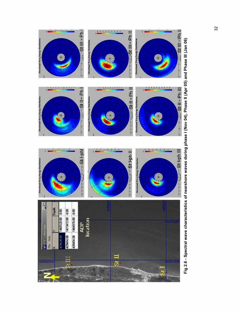
Acoustic Doppler Profiler, which is fitted with pressure sensor. Preliminary PUV analysis was

conducted to study along shore variability of nearshore waves at three stations. Wave

energy distribution from the spectral analysis of PUV records for phase I (November 2004),

phase II (April 2005) and phase III (January 2006) periods are shown in Fig 2.6 and Table

2.2. The directional trend with season is seen at station III, which is 7 km from the port, while

station I and II are influenced by the port. All the field observations indicted that nearshore

circulation is modified by port upo 4 km on northern side and 3 km on southern side with

present configuration of port and intervention (artificial nourishment on north). Attempts

were made to asses the variability of nearshore circulation using numerical model.

32

Fig 2.6 - Spectral wave characteristics of nearshore waves during phase I (Nov 04), Phase II (Apr 05) and Phase III (Jan 06)

34

Table 2.2 - Wave parameters obtained from ADP data for the phases I, II & III

Station I Station II Station III

Wave height

Wave pressure

Wave direction

Wave height

Wave pressure

Wave direction

Wave height

Wave pressure

Wave direction

Phase 1 0.95 6.4 304 0.77 8.7 305 1.46 6.0 249

Phase 2 0.59 9.0 273 0.38 8.4 306 0.32 8.7 291

Phase 3 0.24 9.4 283 0.21 9.4 308 1.15 6.6 232

In Ph I (Nov 04) and Ph III (Apr 05) periods, the waves approach the coast from NE

direction with most of the energy is concentrated in 0.16Hz (6-7sec). During Ph II (Feb 06)

the waves approach the coast from SE with wave energy concentrated at 0.1 to 0.28Hz (4s

& 11s period)

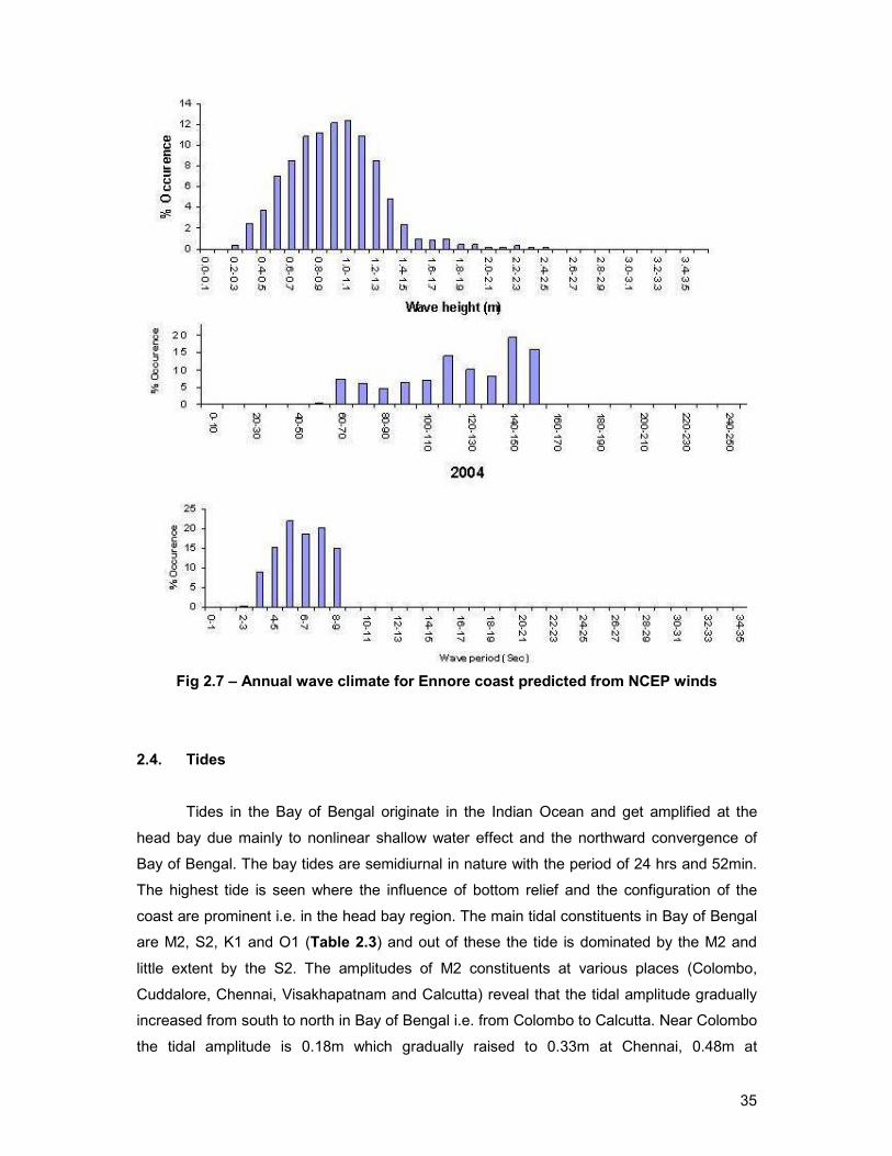
In order to bridge the gap in the wave data of Directional Wave Rider Buoy, NDBP,

annual wave climate derived from Hindcast data was used. NCEP winds at 0.5o grid was

used in Offshore Spectral Wave Model to arrive at wave climate. Predicted waves are

compared with observed data at Ennore and model prediction agrees well in wave heights

and direction but wave periods are under predicted by 15 %. Annual wave climate for the

year 2004-05 is shown in Fig. 2.7.

35

Fig 2.7 – Annual wave climate for Ennore coast predicted from NCEP winds

2.4. Tides

Tides in the Bay of Bengal originate in the Indian Ocean and get amplified at the

head bay due mainly to nonlinear shallow water effect and the northward convergence of

Bay of Bengal. The bay tides are semidiurnal in nature with the period of 24 hrs and 52min.

The highest tide is seen where the influence of bottom relief and the configuration of the

coast are prominent i.e. in the head bay region. The main tidal constituents in Bay of Bengal

are M2, S2, K1 and O1 (Table 2.3) and out of these the tide is dominated by the M2 and

little extent by the S2. The amplitudes of M2 constituents at various places (Colombo,

Cuddalore, Chennai, Visakhapatnam and Calcutta) reveal that the tidal amplitude gradually

increased from south to north in Bay of Bengal i.e. from Colombo to Calcutta. Near Colombo

the tidal amplitude is 0.18m which gradually raised to 0.33m at Chennai, 0.48m at

36

Visakhapatnam and 2.4m at Calcutta. Occurrence of lower tidal amplitude in southern region

of Bay of Bengal is due to presence of amphidromic point (the region of zero tidal range)

around SE corner of Sri Lanka. The phase of the tide also varies from south to north along

Bay of Bengal. At Colombo the phase of the tide is around 50o indicating the tide is

propagating northeastward. From Cuddalore to Visakhapatnam the phase is around 240o

indicating the tide pattern is more or less same and is perpendicular to the coast along

Andhra and Tamil Nadu. Thus the tide propagates from south (Sri Lanka) to north (Calcutta)

in anticlockwise direction once crosses the Sri Lanka region. Very small amplitude of S2

(Table 2.3) compared to M2 indicates the dominance of semi diurnal tidal component along

southern part of East Coast. Thus for Ennore coast the tides are predominantly the semi-

diurnal type with a phase velocity perpendicular to the coast which lead to large scale

seasonal residual circulation along the coast.

Table 2.3 - Amplitudes and phases of tidal components M2, S2, K1 and O1

M2 S2 K1 O1 Places Mean

level Ampli-tude Phase Ampli-tude

Phase Ampli-tude

Phase Ampli-tude

Phase

Colombo 0.38 0.18 50 0.12 101 0.07 36 0.03 59

Cuddalore 0.63 0.26 241 0.11 284 0.10 344 0.02 308

Chennai 0.65 0.33 239 0.14 274 0.09 339 0.03 321

Visakhapatnam 0.84 0.48 239 0.21 274 0.11 336 0.04 320

Calcutta -- 2.41 -- -- -- -- -- --- ---

The tidal characteristics for Chennai coast provided by the Chennai Port Trust are

shown in Table 2.4. All the levels are with respect to chart datum specified by the Naval

Hydrographic Office, India. The change in water levels combined due to astronomical tide,

wind setup, wave set up, barometric pressure, seiches and global sea level rise were

estimated as 1.57m, 1.68m and 1.8m at 15m, 10m and 5m depth contours respectively.

Analysis of the tidal record for Chennai coast reveal that the mean tidal range during spring

tide is 1.0m and during neap tide is 0.4m.

Table 2.4 - Tidal characteristics for Chennai coast

Highest High Water H.H.W 1.50M Mean High Water Spring M.H.W.S 1.10M Mean High Water Neap M.H.W.N 0.80M Mean Sea Level M.S.L 0.54M Mean Low Water Neap M.L.W.N 0.40M Mean Low Water Spring M.L.W.S 0.10M Mean Spring Range M.S.R 1.00M Mean Neap Range M.N.R 0.40M Coastal structures are designed based on wave condition, which is depending on

fluctuation of water levels. They control both flooding and wave exposure. Coastal

37

areas/structures are subjected to larger waves when water level increases. Water level

fluctuation in coastal areas could be due to tides, storm surges, barometric changes and

climatic fluctuations. For modelling of coastal circulation, the role of each forcing function

like tide, wind, wave etc. has to be identified and analysed.

Water levels were monitored at 6 locations in coastal waters and one location inside

the port. The station located inside the port (new finger jetty) was monitored for a period not

less than 30 days in phase II, phase III and phase IV. The data was analysed for harmonic

analysis (Piorewicz, 2002). The pressure data was analysed for separation of tide from non-

tidal components of the signal. The residual time series, amplitudes of various constituents,

spatial contribution of tidal and non-tidal energy are shown Fig. 2.8, Fig. 2.9 and Fig. 2.10

respectively. Analysis of residual time series (detided signal) at Ennore indicate that a signal

with a periodicity of 20days (0.04 to 0.05 cycles per day (cpd)) was observed in all seasons

but during Ph3 and Ph4 a periodicity of 2 cpd was also noticed. In order to study the

influence of meteorological forcing on water level, a continuous observation of

meteorological data (wind speed &direction and pressure) is required. Though, automatic

weather station was deployed at Ennore, continuous data could not be collected due to

frequent failure of power supply at port. Major diurnal, semi-diurnal and quarter-diurnal

constituents derived for the 3 sets of data are shown in Table 2.5.

Spatial variation along tides can be attributed to coastal configuration and presence

of shoals. Asymmetry in tides are seen among different stations (Fig. 2.11) and it is more

predominant during neap phase of the tide.

38

Table 2.5 - Frequencies of selected diurnal, semi-diurnal and quarter-diurnal tidal constituents for phase 2 (Apr. 05), phase 3

(Jan. 06) and phase 4 (Aug. 06)

Phase 2

Phase 3

Phase 4

Type

Tide

constitute

Freq

(cycle/hour)

Amplitude

Phase

Amplitude

Phase

Amplitude

Phase

K1

0.041781

0.1018

334.43

0.0856

326.72

0.1006

337.38

O1

0.038731

0.0331

322.62

0.0268

319.13

0.0281

326.87

Diurnal

P1

0.041553

0.0337

341.5

0.0283

333.79

0.0333

344.45

M2

0.080511

0.3305

235.17

0.3029

219.73

0.32

239.36

S2

0.083333

0.1404

271.89

0.18

259.1

0.1549

271.27

N2

0.078999

0.0629

224.95

0.0765

220

0.0823

241.92

Semi

diurnal

K2

0.083562

0.0382

294.29

0.049

281.5

0.0422

293.67

M4

0.161023

0.0018

7.6

0.0021

47.81

0.0008

119.36

S4

0.166667

0.0014

281.07

0.0011

163.76

0

320.72

MS4

0.163845

0.0008

146.67

0.0021

102.16

0.0038

149.52

Quarter

diurnal

MN4

0.159511

0.0007

277.4

0.0025

42.01

0.001

356.43

39

Fig. 2. 8 – harm

onic analysis of tide at Ennore for ph 2 (Apr 05), ph 3 (Jan 06) and ph 4 (Aug 06)

40

Fig. 2. 9 – Amplitude of analysed tidal constituents with 95% significant level

41

42

Fig. 2.11 – W

ater level variations at different stations (Sts D1, D3, D5, D6 and D7) during Phase I (April 05)

44

2.5 Currents and Circulation

Circulation at Ennore is seasonal and predominantly forced by tide and wind

components. Shankar et al (1996) have studied East Indian Coastal Currents (EICC) and

reported that EICC reverses direction twice a year, flowing Northeastward from February till

September with a strong peak in March-April and Southwestward from October to January

with strongest in November. Major driving mechanism of its variability was attributed to wind

in the Bay of Bengal, which reverses with monsoons. It has also been reported that periods

of peak monsoons do not coincide with times of maximum current speed. Under these

uncertainties, it is difficult to assess the coastal circulation in East Coast. Observations

made under the project on "Waste Load Allocation at Ennore" indicate a sudden reversal in

current direction during the month of March 1999 from south to north.

Based on collated information from other sources and experiences of ICMAM-PD, a

field experiment was designed to monitor the currents at 6 locations between Ennore and

Pulicat. Out of 6 locations, at three locations, the current meters were moored with tide

gauges and rest of the locations were monitored by hanging the instrument from the boat at

water depth of 2 m from surface. All the currents observed at different locations were

analysed.

The stick plot showing the current magnitude for the three phases of observations

are shown in Figs. 2.12 - 2.20. Currents are southerly during NE monsoon i.e., Nov. 04 and

Jan. 05 and northerly for SW monsoon i.e., April 05 and August 2006. The magnitude of the

maximum and mean currents for four phases are given in Table 2.6.

46

Table 2.6 - Spatial Distribution of Current Magnitude and Direction at various stations (for the 4 phases of observations)

Phase I

Phase II

Phase III

Phase IV

Location/

Station

Average

(cm/sec)

Maxim

um

(cm/sec

Direction

Average

(cm/sec)

Maxim

um

(cm/sec

Direction

Average

(cm/sec)

Maxim

um

(cm/sec

Direction

Average

(cm/sec)

Maxim

um

(cm/sec

Direction

D1

h=2.5, H=10

20

45

SW

20

32

NE

4

6

NE & SW

--

--

--

D2

h=9.2, H=20

15

25

SW & NE

--

--

--

--

--

--

--

--

--

D3

h=4.2, H=6.5

25

48

S

20

30

N

18

25

N

--

--

--

D5

h=2.7, H=22

30

50

S

45

70

N

25

35

NNE

40

55

N

D6

h=2.6, H=10

25

65

S

30

35

N

15

22

N

--

--

--

D7

h=9.0, H=19

35

60

S

40

55

N

--

--

--

--

--

--

58

Fig 2.12 - Measured currents at Station D1, South of Ennore Port (Phase 1 - Nov. 04)

59

Fig. 2.13 - Measured currents at Station D3, North of Ennore Port (Phase 1 - Nov. 04)

60

Fig. 2.14 - Measured currents at Station D4, North of Ennore Port (Phase 1 - Nov. 04)

61

Fig. 2.15 - Measured currents at Station D1, South of Ennore Port (Phase 2 - Apr. 05)

62

Fig. 2.16 - Measured currents at Station D3, South of Ennore Port (Phase 2 - Apr. 05)

63

Fig. 2.17 - Measured currents at Station D6, South of Ennore Port (Phase 2 - Apr. 05)

64

Fig. 2.18 - Measured currents at Station D1, South of Ennore Port (Phase 3 - Jan. 06)

65

Fig. 2.19 - Measured currents at Station D6, North of Ennore Port (Phase 3 - Jan. 06)

66

Fig. 2.20 - Measured currents at Station D6, North of Ennore Port (Phase 3 - Jan. 06)

67

Acoustic Doppler Velocimeter (ADV) (5 MHz) was deployed in nearshore area at a

water depth of 3 - 6 m on either side of the Port to monitor mean currents, wave orbital

velocities and turbulent velocities. The directional spectrum derived from p, u, v analysis

based on Extended Maximum Entropy Principle (EMEP) method (Hashimoto, N, 2002).

The three parameters required for the analysis are sampled at 4 Hz with 1024/2048 samples

with a measuring interval of 30 minutes. The parameter 'p' from the pressure sensor and 'u,

v' from the velocimeter located at a height of 1.1 m from the seabed. The result from the

directional spectrum analysis at 3 stations, namely, station 1 (south of Ennore Port), station

2 (immediate north of Ennore Port) and station 3 (2 km from north of station 2 at Kalanji) are

shown in Fig.2.21. Stations 2 & 3 show nearshore currents coincided with coastal currents

and its direction is northerly during southwest monsoon and southerly during northeast

monsoon. But, station 1, which is located at 500 m south of Ennore Port, is influenced by

Ennore breakwaters, do not show any particular trend in the direction.

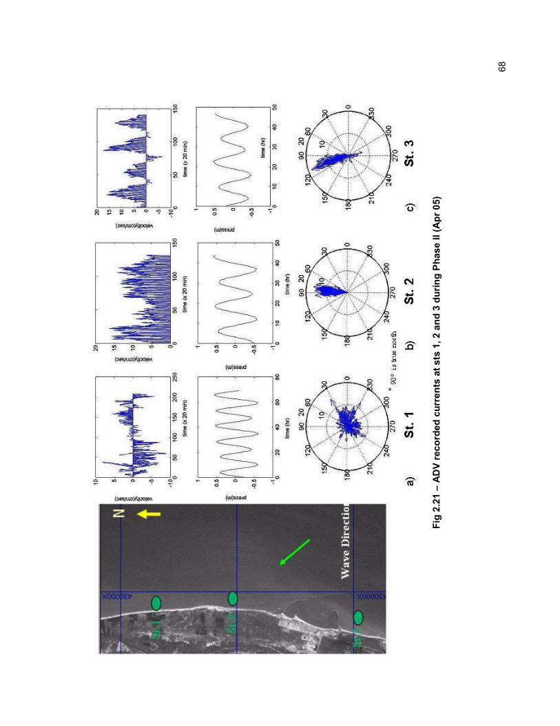
68

Fig 2.21 – ADV recorded currents at sts 1, 2 and 3 during Phase II (Apr 05)

69

2.6 Suspended Sediment Distribution

Plot of suspended sediment concentrations for phase I (Nov 04), phase II (Apr 05)

and Phase III (Jan 06) periods is shown in Fig 2.22. In phase I & II (Fig 2.22a) the isolines

are more closely packed in the region just immediate N & NE of northern breakwater

(Ennore port), indicating the presence of high concentration of suspended sediment.

Presence of high concentration (12 – 18 mg/litre) on north of Ennore port may be due to

generation of turbulence related to the presence of Ennore shoals or port structures. It is

observed that the suspended sediment concentration decreased offshore i.e. as one goes

away from the port region. Near the shoreline, the concentration is about 8.5-18.1 mg/litre

while at 20m depth contour (around 7km offshore) the concentration reduced to 6.6 – 8

mg/litre. It is also noticed that the suspended sediment concentration decreased along the

coast as one goes away from the port region; on northern side the concentration decreased

from 18.1 mg/litre (near northern breakwater) to 8.5mg/litre (near Pulicat mouth). On

southern side it decreased from 12.3mg/litre (southern breakwater) to 10mg/litre (near

Ennore creek). It is clearly noticed that the suspended sediment movement has a tendency

to move along the coast northward during phase II and southward during Phase I & III

periods. Thus the suspended sediment movement is driven by the seasonal coastal

currents.

70

Fig. 2.22 - Suspended sedim

ent concentration (mg/l) a) Phase I, b) Phase II and c) Phase III (Hypothetical track of ssd m

ovement)

71

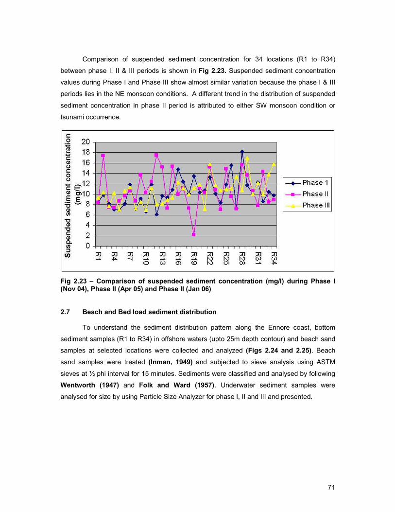
Comparison of suspended sediment concentration for 34 locations (R1 to R34)

between phase I, II & III periods is shown in Fig 2.23. Suspended sediment concentration

values during Phase I and Phase III show almost similar variation because the phase I & III

periods lies in the NE monsoon conditions. A different trend in the distribution of suspended

sediment concentration in phase II period is attributed to either SW monsoon condition or

tsunami occurrence.

Fig 2.23 – Comparison of suspended sediment concentration (mg/l) during Phase I (Nov 04), Phase II (Apr 05) and Phase II (Jan 06) 2.7 Beach and Bed load sediment distribution

To understand the sediment distribution pattern along the Ennore coast, bottom

sediment samples (R1 to R34) in offshore waters (upto 25m depth contour) and beach sand

samples at selected locations were collected and analyzed (Figs 2.24 and 2.25). Beach

sand samples were treated (Inman, 1949) and subjected to sieve analysis using ASTM

sieves at ½ phi interval for 15 minutes. Sediments were classified and analysed by following

Wentworth (1947) and Folk and Ward (1957). Underwater sediment samples were

analysed for size by using Particle Size Analyzer for phase I, II and III and presented.

72

Fig. 2.24 - Bedload sedim

ent size (mm) a) Phase I b) Phase II and c) Phase III

73

Fi

Fig. 2.25 – Beach sand size (m

m) along Ennore coast for a) Phase I (Nov 04), Phase II (Apr 05) and Phase III (Dec 05)

82

Ennore sediments fall under coarse (1.0 - 0.5 mm) to medium (0.5 - 0.25 mm) sand

class where medium grained sand is predominant. In general, the sands are moderately well

sorted to moderately sorted, positive to negatively skewed but predominantly symmetrical

during SW monsoon and negatively skewed during NE monsoon indicating excess of fines,

platykurtic to leptokurtic, majority being mesokurtic. In general, the sand characters indicate

a relatively medium energy environment along this stretch.

Alongshore and cross-shore variations in sand characters are not showing any

particular trend in relation to littoral drift. This could be attributed to varying levels of wave

energy and alternative zones of convergence and divergence along the shore and it may

also be due to the reversal of nearshore currents owing to NE and SW monsoons.

In general, the grain size of bottom sediment varied between 0.01 to 0.7 mm with an

average of 0.32 mm. Bottom sediments in offshore waters are predominantly of silt and to a

lesser extent clay except in the region of shoal where medium size sand was noticed.

Relatively higher grain size probably derived from beach fill area and may be transported

and got deposited in the direction of NE where they come across shoals. Higher size may

also be due to the lifting of fines and leaving behind the coarse when waves encounter the

shallow depths (shoals) suddenly which leads to turbulent effects. However, both the

reasons need confirmation based on detailed mineralogical studies.

The Coarser and moderately sorted sediments with symmetrical nature at north of

the port are favorable for longevity of nourishment. However all along the beach, the sand is

mainly medium to coarse grained and moderately sorted and their size varied from 0.31 to

0.75mm.

Comparison of sediment size for different stations (R1 to R34) for three phases (Fig.

2.26) show more or less similar features except in the region from Kalanji to Satankuppam

stretch (sts R11 to R21) where the orientation of the coast and relatively more deeper depths

compare to adjacent nearshore areas may influence the pattern of sand. On the whole the

sediment sizes of 0.22mm (2.1φ) to 0.33 mm (1.32φ) are most predominant along the beach

and 0.11mm (3.14φ) in offshore areas.

83

Fig 2.26 – Comparison of grain size (phi) for Sts R1 to R34 for a) Phase I (Nov 04), b) Phase II (Apr 05) and Phase III (Dec 05)

In order to study the qualitative and quantitative aspect of sediment deposition,

locally made sand traps were deployed at 4 stations (Sts D1, D3, D5 & D6) during phase III

(Dec 05) period. Analysis of the sediment collected in sand traps (Fig 2.27) reveal that St D6

shows entirely different trend in sedimentation than the other 3 stations. Sts D1 and D5 (Fig.

2.27) show similar characteristics of sediment which indicate that most of the sediment

transport is by passing from south of Ennore port (from St. D1) to offshore area in the NE

direction where St D5 is located. St D3 shows mixed trend of sediment distribution pattern

which may be due to erosion and spreading of beachfill material. Distribution of settling rates

of sediment at different stations (Fig 2.27b) indicate that sts D1 and D5 show more or less

similar rates. St D6 show more sediment settling rate compared to the other stations.

84

Fig 2.27 – Distribution of a) settling rate (grams/hr) and b) sediment size (microns) at different stations during phase II (Dec 05) 2.8 Littoral Environmental Observations

Field observations on littoral parameters (Breaker ht, period, longshore current speed

and direction, breaker angle etc.) along Ennore coast were made during phase I, Phase II

and Phase III periods. Results are presented and discussed below.

Zone I (Ennore port area): Field observations on Littoral Environmental parameters along

north and south of Ennore port during Phase I, Phase II and Phase III periods (Table 2.7)

are presented below.

85

North of Ennore port: The northern shore of Ennore port is occupied predominantly

with spill breakers of height 0.2-1.7m under Phase I, 0.3-1.3m under Phase II and 0.2-1.0m

under phase III. Much of the incoming wave energy is expended in breaking before it

reaches the shoreline indicating dissipative beach. Surf zone is wide along this zone due to

the presence of shoals. Occasionally, wave breaking is noticed on immediate north due to

the shoals. The strength of the longshore currents is 0.01-0.14m/s under Ph I; 0.08-0.24m/s

under Ph II; and 0.05-0.12m/s under Ph III. The direction of longshore current is

predominantly southward during Ph I & III (NE monsoon condition) periods and northward

during Ph II (SW monsoon condition) period even though at some places bi-directional

longshore current occur.

South of Ennore port : The southern shore is predominant with plunging type of

breakers, having heights of 0.3-2.0m under Phase I, 0.3-1.3m under Ph II and 0.3-1.6m

under Phase III. Along this stretch within 1 km from south breakwater, the waves break

almost on the beach leading to reflective beach. Surf zone is very narrow along this stretch.

Beyond 1km south, breaking of waves occur before reaching the coast indicating dissipative

beach. The strength of the longshore currents are 0.02-0.14m/s under Ph I; 0.07-0.15m/s

under Ph II; and 0.10-0.15m/s under Ph III. The direction of Longshore current is southward

under Ph I & III (NE monsoon condition) periods while northward under Ph II (SW monsoon

condition).

On the whole the beach on the northern side of port is dissipate beach occupying

with spill breakers. However, the beach on southern side is reflective beach predominant

with plunging breakers. Along north coast the spillers run long distance before reaching the

shore while on south coast plungers breaking almost at shore. Thus Breaker zone is wider

on north while narrow on south; Wave crests approaching shore with higher angle on north

when compared with that on south; On north, much of the incoming wave energy is

expended in breaking before it reaches the shoreline indicating dissipative beach, However

on south the waves breaking almost nearer to shoreline with grater height indicating

reflective beach.

86

Table 2.7a– Littoral environmental observations along Ennore coast during Phase I (Nov 04)

Phase I

Location Breaker type

Breaker height (m)

Breaker period (Sec)

Breaker angle

LSC Speed (m/s)

LSC dir

Zone I

North of Ennore port

spilling 1.0-1.7 (foreshore)

0.2-0.8 (nearshore)

6 to 11 10-15o 0.01 – 0.14 south

South of Ennore port

Plunging &Spilling

1.5-2.0 (foreshore) 0.3-1.0

(nearshore) 6 to 11 5-7o 0.02 – 0.12 south

Zone II North

Kattupalli to light house

Plunging & spilling

1.2-2.5 (foreshore) 0.2-0.7

(nearshore) 5 to 12 3 to 7o 0.02-0.21 Oscillatory

Zone III

South of Pulicat mouth

Plunging & spilling

1.8-2.5 (foreshore) 0.2-0.4

(nearshore) 6 to 9 3 to 7o 0.02-0.3 Oscillatory

North of Pulicat mouth

spilling

0.8-1.5 (foreshore) 0.2-0.4

(nearshore)

4 to 9 5 to 9o 0.02-0.04 north

Zone II (Between Kalanji & Satankuppam): The region is usually occupied with

submerged shoals in the surf zone. Initially the breakers start as plungers at seaward end of

surf zone, once they reach the shoal area they become spill breakers. Along this stretch the

breakers (wave crests) approach the shoreline in bidirections from SE and NE. Breaker

height varied from 0.2 to 2.5m in phase I, 0.4 to 1.0m in phase II and 0.2 to 0.8m in phase III.

The bi-directional approach of waves leads to an oscillatory long shore current that runs

sometimes northward and southward with varying speeds between 0.02 and 0.21m/s. The

shoreline is occupied with sand backed shore line and there is no sand dunes. Since the

majority of the surf zone occupied with spill breakers of varying heights this beach is also

dissipative beach.

87

Table 2.7b – Littoral environmental observations along Ennore coast during Phase II (Apr 05)

Phase II

Location Breaker type

Breaker height (m) Breaker period (Sec)

Breaker angle

LSC Speed (m/s)

LSC dir

zone I

North of Ennore port

plunging

1.2 - 1.7(foreshore) 0.3-0.5(nearshore)

7 to 10 10 to 15 0.08 - 0.24 north

South of Ennore port

spilling 1.0 - 1.3 (offshore) 0.3 – 1.0(nearshore)

6 to 8 8 to 9 0.07 - 0.15 north

Zone II North Kattupalli to light house

plunging

1.3 - 1.5 (foreshore) 0.4-0.7(nearshore)

7 to 8 13 to 17 0.12 to 0.13

north

zone III South of Pulicat

mouth plunging

1.2 - 1.5 (foreshore) 0.3 – 0.5 (nearshore)

8 to 9 15 to 18 0.1 - 0.3 north

North of Pulicat mouth

spilling 1.0 - 1.2 (foreshore) 0.2-0.5 (nearshore)

7 to 9 15 to 20 0.12 - 0.24 north

Zone III (Pulicat confluence): The north shore is very flat and wider and occupied

with mostly spill breakers of heights 0.2-1.5m. Littoral currents speeds of the order of 0.02 to

0.3m/s moving in north direction. The south shore of Pulicat confluence is mainly

depositional shore and occupied with a small bay like formation. Plunging wave heights of 2-

2.5m at Seaward end of breaker zone and spillers of height 0.2-0.4m in the surf zone are

noticed. Longshore current is oscillatory i.e. northward sometimes and southward in other

times because of bi-directional approach of wave crests from NE & SE directions.

Table 2.7c – Littoral environmental observations along Ennore coast during Phase III (Dec 05)

Phase III

Location Breaker type

Breaker height (m)

Breaker period (Sec)

Breaker angle

LSC Speed (m/s)

LSC dir

Zone I

North of Ennore port

spilling

0.5-1.0 (foreshore) 0.2-0.5

(nearshore)

5 to 7 10-15o 0.05 – 0.12

southward

South of Ennore port

Plunging &Spilling

1.2-1.6 (foreshore) 0.3-1.0 (nearshore)

7 to 9 10 to 12o 0.10 to 0.15

southward

Zone II North

Kattupalli to light house

Plunging & spilling

0.7-1.0 (foreshore) 0.2-0.8 (nearshore)

6 to 8 5 to 10 0.05 to 0.12

southward

Zone III

88

Phase III

Location Breaker type

Breaker height (m)

Breaker period (Sec)

Breaker angle

LSC Speed (m/s)

LSC dir

South of Pulicat mouth

Plunging & spilling

0.5-0.9 (foreshore) 0.2-0.4 (nearshore)

6 to 9 3 to 7 o 0.02-0.09 southwar

d

North of Pulicat mouth

spilling 0.8-1.0(foreshore)

0.2-0.6(nearshore)

4 to 9 5 to 9 o 0.02-0.04 oscillator

y

On the whole it is observed that during SW monsoon period the longshore current

velocities are relatively high compared to that during NE monsoon period. The littoral

currents are directed to north along the coast during SW monsoon conditions and south

during NE monsoon conditions (Fig 2.28).

89

Fig 2.28 – Hypothetical picture of littoral processes during a) NE m

onsoon (Nov 04) and b) SW m

onsoon (Apr 05)

90

2.9 Beach Profile Changes

The Ennore coastline is typical in its orientation. From Ennore creek to Kattupalli the

shoreline orients in the direction of 170 N where as from Kattupalli onwards it orients in

350oN. This 27o change in shoreline orientation may lead to wide variation in nearshore

sediment transport pattern. In order to study the seasonal variation in sediment transport

pattern and to identify the erosion/ deposition cells, number of cross-shore beach profiles

(Tn3 to Tn25) at a number of transects along Ennore coast (Fig 2.29) were measured with

RTK. These profiles were then reduced to chart datum and the variation in cross-sectional

volume across 25 profiles were computed for phase I (Nov 04), phase II (Apr 05) and Phase

III (Dec 05) periods (Table 2.8).

91

Fig 2.29 a – Station locations for beach profiles along Ennore coast

92

Fig 2.29b – Beach profiles at selected locations along Ennore coast

93

Fig 2.29c – Beach profiles at selected stations along north coast of Ennore port

Seasonal variations as well as role of tsunami run up on beach sediment volume

changes were studied. The main features identified were i) From November 2004 to

December 2005, occurrence of series of erosional and depositional zones on north coast

beyond beach fill (Tn 7 to Tn 25) indicate that the beach changes resembles more natural

phenomena. However the Kalanji shore (tn13 to tn17 transects) showing continuous erosion

by showing decreased sediment volume and ii) The cross-sectional sediment transport

varied from 2 to 117 cu.m/m/year depending upon the location.

94

Table 2.8 – Sediment volumes (cu.m/m) at selected transects along Ennore coast

Track Latitude Longitude Nov 04 Mar 05 Dec 05 Nov 04-Mar 05

Mar 05-Dec 05

Annual Variation

TN25 1483910 427286.9142 266 270 256 4 -14 -10

TN24 1483159 427270.4882 313 325 418 12 93 105

TN23 1481491 427472.8466 102 99 89 -3 -10 -13

TN21 1480699 427465.2483 287 270 255 -17 -15 -32

TN20 1480033 427758.7453 76 66 69 -10 3 -7

TN19 1479435 427824.6185 99 109 117 10 8 18

TN18 1478992 427914.1009 114 129 164 15 35 50

TN17 1478560 428011.9487 215 238 211 23 -27 -4

TN16 1478134 428202.5162 105 97 90 -8 -7 -15

TN15 1477628 428261.9114 215 194 190 -21 -4 -25

TN14 1477191 428397.0448 170 162 150 -8 -12 -20

TN13 1476654 428548.9997 185 172 146 -13 -26 -39

TN12 1476085 428656.9478 170 165 168 -5 3 -2

TN11 1475426 428811.7162 17 60 29 43 -31 12

TN10 1473536 429059.6449 82 64 59 -18 -5 -23

TN9 1470809 429106.3154 344 405 364 61 -41 20

TN8 1470523 429131.1599 367 369 373 2 4 6

TN7 1469983 429136.4404 275 314 283 39 -31 8

TN5 1469026 428870.4828 1095 1243 1212 148 -31 117

TN4 1468896 428812.8325 972 1155 896 183 -259 -76

TN3 1468565 428874.9552 319 366 373 47 7 54

TN2 1468474 428832.4553 344 407 364 63 -43 20

In order to understand the role of recent tsunami (26 th Dec 04) run up on sediment

transport along the Kattupalli area, the available 4 beach profiles (Fig 2.30) before (Nov

2004) and after tsunami (Feb 2005) were analyzed. The increase in sediment volume in

post-tsunami period (Table 2.9) indicates adding up of the sediment to the shore which may

be due to normal seasonal sediment transport pattern or tsunami run up (occurred just one

month back). The beach profiles comparison in Fig 2.30 clearly reflect that the backshore

region faced accumulation of sediment in all profiles and the foreshore region shows erosion

trend. Thus It is believed that the foreshore sediment is lifted by tsunami run up and

deposited on the backshore. An amount of 0.2 to 18 m3/m of sediment was added along the

back shore of Kattupalli area.

95

Fig 2.30 – Comparison of beach profiles at 4 transects before and after tsunami run up along north Kattupalli coast

96

Table 2.9 – Cross-sectional volumes (m3/m) at 4 transects before and after tsunami along Kattupalli coast

Profile Id Nov. 04 Feb. 05 Volume change

9A 161 161.2 0.2

9B 48.3 43.7 -4.6

9C 93 102 9.0

9D 117 134 18.0

2.10 Shoreline Changes

To study the historical as well as seasonal variations in shoreline changes along

Ennore coast, the shoreline position data collected by PWD, Chennai during 1984 – 2004

and the field data collected by the ICMAM-PD from 1999 onwards were analyzed and the

results are presented below.

97

Fig 2.31 – Historical changes in shoreline position

Table 2.31 – Historical changes in shoreline position

Tracks Range of shift (m/year)

PO1 -19 to +17

PO2 -30 to +24

PO3 -35 to 54

PO4 -81 to 89

98

Historical trend: The concept of setback line has been adopted in many countries to

regulate the developments in near coast. State Public Works departments, Tamil Nadu is

monitoring the shoreline oscillations along the Tamilnadu coast under the monitoring

program called “Crest of the Berm”. The crest berm is seaward end of the beach profile,

formed by the action of waves and found to be ideal feature for assessing the shoreline

change. The crest of the berm data from 1984 to 2004 (20 years) was analysed to compute

the shoreline oscillation along the Ennore coast. The shoreline changes at 4 selected sts

PO1, PO2, PO3 & PO4 (Fig. 2.31) along Ennore coast reveal that from 1984 to 1993 the

shoreline oscillates mostly both seaward or land ward where as from 1994 onwards the

shore shifted mostly to landward at PO1, PO2 & PO3 and seaward at PO4. On the whole the

historical changes in shoreline data indicate that the shore usually migrates from –20 to

+90 m per annum (Table 2.31) along Ennore coast depending upon the location.

Recent trend: The recent field observations of shoreline position for different

periods during 1999 to 2006 were shown in Fig. 2.32. The positions were measured

based on berm crest location using RTK GPS. The shoreline positions were plotted

on a rectified satellite image in Arcview software and the changes, if any, in shoreline

position and the corresponding erosional/ depositional trends were identified. The

distance of migration either seaward (deposition length) or landward (erosion length)

were measured with the help of Arcview GIS software. In determining the exact rate

of erosion or deposition, care was taken whether the coast was exhibiting any

abnormal variation other than seasonal variation. In determining the erosion zone the

continuos migration of shoreline landward was taken into account. The shoreline

changes obtained in this way reveal the following features.

99

Fig 2.32a – Shoreline migration near Pulicat mouth during 1999 to September 2006

Fig 2.32b – Shoreline migration at south of Pulicat mouth during 1999 to September 2006

100

Fig 2.32c – Shoreline migration at Kalanji during 1999 to September 2006

Fig 2.32d – Shoreline migration at south of Kalanji during 1999 to September 2006

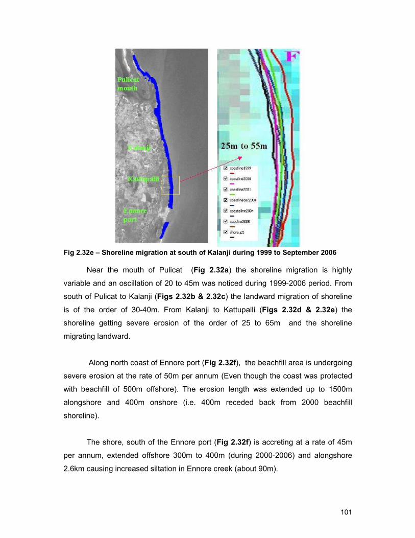
101

Fig 2.32e – Shoreline migration at south of Kalanji during 1999 to September 2006

Near the mouth of Pulicat (Fig 2.32a) the shoreline migration is highly

variable and an oscillation of 20 to 45m was noticed during 1999-2006 period. From

south of Pulicat to Kalanji (Figs 2.32b & 2.32c) the landward migration of shoreline

is of the order of 30-40m. From Kalanji to Kattupalli (Figs 2.32d & 2.32e) the

shoreline getting severe erosion of the order of 25 to 65m and the shoreline

migrating landward.

Along north coast of Ennore port (Fig 2.32f), the beachfill area is undergoing

severe erosion at the rate of 50m per annum (Even though the coast was protected

with beachfill of 500m offshore). The erosion length was extended up to 1500m

alongshore and 400m onshore (i.e. 400m receded back from 2000 beachfill

shoreline).

The shore, south of the Ennore port (Fig 2.32f) is accreting at a rate of 45m

per annum, extended offshore 300m to 400m (during 2000-2006) and alongshore

2.6km causing increased siltation in Ennore creek (about 90m).

102

Fig 2.32f – Shoreline m

igration on north and south of Ennore port during 1999 to September 2006

103

3. MODELING

The objective of modelling is develop impact models to evaluate various

management options in terms of its functionality and cross impacts resulted from the

interventions proposed under each management strategy. The dynamics of the coastal

waters were analysed based on the field observations conducted for a period of one year,

covering all seasons on various parameters such as water levels, currents, wave climate,

sediment transport, shoreline oscillations etc. The following models are being used to

generate impact models

i) Hydrodynamic Model to simulate flow pattern

ii) The Offshore Spectral Wave and Parabolic Mild Slope wave models for deriving

wave climate

iii) MIKE 21 ST module for sediment transport pattern and bed level changes and

iv) LITPACK model for prediction of shoreline changes. The preliminary results of the

model investigations are summarized and presented below.

3.1 Hydrodynamic Model

In order to simulate water levels and current pattern for Ennore coast, the

hydrodynamic (HD) module of MIKE 21 was setup. The HD model simulates water level

variations and flows in coastal regions. The model can account bottom friction, wind effect,

coriolis force, sources and sinks and wave radiation stresses. For Ennore coast, the model

area considered for the simulation is 14km x 8km (Fig. 3.1a), covering 7 km coast on north

of Ennore Port and 4 km on south. The seaward boundary is extended upto 25 m depth

contour and the landward boundary upto shoreline. A 10m x 10m grid was discretized from

the measured bathymetry. Three open boundaries were considered in the simulation i.e. the

north and south boundaries are provided with water levels and the eastern boundary with

water flux as a function of time. Since the coast, experiences seasonal reversal of circulation

pattern, the model simulations were carried out for NE and SW monsoon conditions (Fig 3.1

b & c). The model was calibrated with field data for phase I, II & III periods and the

circulation pattern around port area was simulated.

104

Fig. 3.1 - a) Bathymetry and b) & c) Sim

ulated water levels and currents under NE m

onsoon (Nov. 04) and SW m

onsoon (Apr. 05)

respectively

105

The simulated water levels are well correlated with observed ones (Figs. 3.2 & 3.3).

The two major forcing functions, i.e., tide and wind, influence the circulation pattern, latter

being a dominant forcing function, which control the direction of current. The flow field south

of Ennore Port is complex and field observations indicate no distinct pattern. The circulation

north of Port is influenced by long north breakwater and presence of shoals.

106

Fig. 3.2 - Comparison of predicted and observed tide under NE m

onsoon (Nov. 04)

107

Fig. 3.3 - Comparison of predicted and observed tide under SW m

onsoon (Apr. 05)

108

3.2. Wave Model

Spectral wind–wave model (OSW): In order to predict the annual wave climate for

Ennore coast, the spectral-wind wave model, the OSW was used. The basic requirement for

the model are i) wind data, which was obtained from NCEP winds and ii) the bathymetry,

which was derived from C-MAP. The model was run initially by using the NCEP winds to get

global wave climate. Boundary wave climate for Ennore coast was extracted and provided

as input to PMS model to simulate nearshore waves by giving the extracted waves as

offshore boundary. Finally the model was calibrated with the field observations (Fig 3.4) and

utilized to study the annual variations in nearshore wave climate.

Fig 3.4 – Comparison of OSW predicted waves with observed ones

109

Fig 3.5 – Predicted annual wave record for Ennore offshore waters (OSW model)

The annual distribution of wave record (Fig 3.5) indicates that during Nov – Dec the

waves are mostly from 60o-70o in other months from120-140o. Percentage distribution of

wave directions (Fig 3.6) clearly shows that almost 85% of waves are coming from E-SE

(90-160o) direction and the remaining 15% are from NE-ENE (40-80o). Thus the annual

Ennore wave climate leads to a net northward littoral sediment transport pattern over a year.

Wave periods varied between 3 to 9 sec and heights from 0.5 to 2.0m. Most percentage of

waves occurs in the height range 1.0 to 1.5m and in the periods of 4-9 sec.

110

Fig 3.6 – Percentage occurrences of a) wave ht (m), b) Wave dir. (deg) and c) wave pr. (s) for annual wave record of Ennore coast

Nearshore Wave Model: To study the wave transformation from offshore to

nearshore region in the Ennore coastal waters is simulated using Parabolic Mild Slope

(PMS) wave model of MIKE 21. The model is a linear refraction-diffraction model based on

a parabolic approximation to the elliptic mild slope equation. The model takes into account

the effects of refraction and shoaling due to varying depth, diffraction along the

perpendicular to the predominant wave direction and energy dissipation due to bottom

friction and wave breaking. The presence of shoals on north of Ennort Port requires

diffraction model. The model also considers the effect of frequency and directional spreading

using linear superposition. For Ennore coast, the model was run to study the wave

transformation from 25 m depth to nearshore coast. The study area and the bathymetry are

111

the same as that used in HD simulation. The offshore boundary is specified with time series

of observed wave parameters (RMS wave ht, mean wave direction and peak period). The

two lateral boundaries (North & south) are considered with the symmetry type of boundary

condition, for which the depth contours are assumed to be straight and parallel at the

boundaries. Model simulations were conducted by using the field data of Phase I, Phase II

and Phase III periods. The results are presented in Fig 3.7.

1 meter

Hrms [m] (meter)

Above 0.880.84 - 0.880.8 - 0.840.76 - 0.80.72 - 0.760.68 - 0.720.64 - 0.680.6 - 0.640.56 - 0.60.52 - 0.560.48 - 0.520.44 - 0.480.4 - 0.440.36 - 0.40.32 - 0.360.28 - 0.320.24 - 0.280.2 - 0.240.16 - 0.20.12 - 0.160.08 - 0.120.04 - 0.080 - 0.04

-0.04 - 0Below -0.04

F:\fresh-pms\ph2-d5d3-port\result\rotph2wave.dfs2

0.0 2.0 4.0 6.0(kilometer)

0

1

2

3

4

5

6

7

8

9

10

11

12

13

14(kilometer)

Fig 3.7a – Simulated wave ht (m) and direction for SE waves

112

1 meter

Hrms [m] (meter)

Above 1.151.1 - 1.151.05 - 1.11 - 1.05

0.95 - 10.9 - 0.950.85 - 0.90.8 - 0.850.75 - 0.80.7 - 0.750.65 - 0.70.6 - 0.650.55 - 0.60.5 - 0.550.45 - 0.50.4 - 0.450.35 - 0.40.3 - 0.350.25 - 0.30.2 - 0.250.15 - 0.20.1 - 0.150.05 - 0.10 - 0.05

Below 0

F:\fresh-pms\ph3-d5d3-port\result\rotph3wave.dfs2

0.0 2.0 4.0 6.0(kilometer)

0

1

2

3

4

5

6

7

8

9

10

11

12

13

14

(kilometer)

Fig 3.7b – Simulated wave ht (m) and direction for E waves

113

1 meter

Hrms [m] (meter)

Above 1.261.2 - 1.261.14 - 1.21.08 - 1.141.02 - 1.080.96 - 1.020.9 - 0.960.84 - 0.90.78 - 0.840.72 - 0.780.66 - 0.720.6 - 0.660.54 - 0.60.48 - 0.540.42 - 0.480.36 - 0.420.3 - 0.360.24 - 0.30.18 - 0.240.12 - 0.180.06 - 0.120 - 0.06

-0.06 - 0-0.12 - -0.06Below -0.12

11/21/2004 22:30:00

F:\fresh-pms\ph1-d5d3-port\ph1waverot.dfs2

Scale 1:53610

0.0 2.0 4.0 6.0(kilometer)

0

1

2

3

4

5

6

7

8

9

10

11

12

13

14

(kilometer)

Fig 3.7c – Simulated wave ht (m) and direction for NE waves

114

Simulations were conducted for predominant wave directions prevailing at Ennore,

namely, ENE-60o, E-90o and Southeasterly waves (135o) (Fig. 3.7). The coast south of Port

experiences diffracted waves during NE monsoon and refracted waves during SE monsoon.

High concentration of wave energy is noticed at south of Port during SW monsoon. The

coast north of Port experiences concentration of wave energy at some places due to

convergence of wave rays resulting from complex bathymetry (shoals). Simulated wave

heights were compared well with the observed heights with an rms error of 0.1 and

correlation coefficient greater than 0.76 (Figs 3.8 and 3.9).

115

Fig 3.8 – Comparison of observed and sim

ulated wave heights a) Phase I (Nov 04), b) Phase II (Apr 05) and c) Phase III (Dec 05)

116

Fig 3.9 – Comparison of observed and sim

ulated wave heights at sts D3, D4 and D5

117

3.3 Sediment Transport Model

MIKE 21 ST (Sediment Transport) module is used for simulation of sediment

transport rates along the Ennore coast. The model calculates the rates of non-cohesive

sediment (sand) transport for combined waves and current situations. Apart from the

sediment transport components, the model also simulates the initial rates of bed level

changes. The basic requirements for the model simulation are i) the Wave climate and

radiation stresses derived from MIKE 21 PMS model results (Fig. 3.7) of section 3.2, ii) The

flow pattern derived from MIKE 21 HD simulation (Fig 3.10), and iii) Preparation of sediment

table based on sediment size distribution of the model area. By giving the appropriate inputs,

ST model was run for Phase I, II & III periods and the results were used to identify the

potential areas of erosion and deposition and the initial rate at which bed level changes (Fig.

3.11).

118

Fig 3.10a – Wave induced currents (cm/s) under SE waves used in ST model

119

Fig 3.10b – Wave induced currents (cm/s) under NE waves used in ST model

The model results indicate that the nearshore waters of beachfill area are

experiencing maximum sediment transport (of about 183 cu.m/yr/m) rates compared to other

regions. This may be due to concentration of wave energy associated with wave

convergence in the presence of port structures. At other places the sediment transport is of

the order of 20-50 cu.m/yr/m.

120

Fig. 3.11a – Domain of sediment transport rates and initial bed level changes under SE waves

121

Fig. 3.11b – Domain of sediment transport rates and initial bed level changes under NE waves

122

The offshore extension of sediment transport zone is also varied from place to place

depending upon the wave convergence and divergence zones. The transport zone extended

upto 0.5 to 1.5km offshore near beachfill area and upto 0.1 to 0.3km in other places.

However, a detailed modeling investigations are required, when an appropriate intervention

is finalized.

3.4 Shoreline model (LITPACK)

To simulate shoreline evolution along Ennore coast, the one dimensional model

LITLINE of LITPACK system was used. The model has the capacity to simulate the

influence of structures like groin, breakwater, jetties etc on shoreline evolution and has the

facility to include sediment source and sinks. The model predicts variations in shoreline

position with in a stipulated period of time under the combined action of waves and currents.

The input data required for the model are cross-shore profile, initial shoreline position along

the coast, sediment size, annual wave climate etc. The required annual wave climate for

Ennore coast is derived from the OSW/PMS model simulations discussed under section 3.2.

The cross-shore profiles and the shoreline positions used in LITPACK model were derived

from the RTK field data collected on different occasions during 1999-2005. As the Ennore

coastline is subjected to changes due to natural and man-made activities (historical changes

of Ennore coast is discussed section 3.0), the LITLINE simulations (Fig 3.12) were carried

out for 3 Cases – I) shoreline evolution under the condition of no port structures i.e. with

the1999 shoreline as base; ii) Shoreline evolution under the presence of port structures with

1999 shoreline as base and iii) Shoreline evolution of beach filled shore with 2001 shoreline

as the base.

123

Fig. 3.12 - Shoreline changes under a) No Port, b) Port and c) beachfill

124

Simulations and field observations indicate that the beachfill placed north of Port was

lost upto an extent 70% and the prediction indicates entire beachfill be subjected to erosion

by the year 2007 (Fig 3.13). After 2007, the natural coast will start eroding (Fig 3.14) if no

sand is supplied. Simulations also indicate that shallower parts of the shoals (water depth of

less than 6 m) are also likely to be eroded.

125

Fig 3.13 – Predicted and observed shoreline along north and south coast of Ennore

126

Fig 3.14 a– Predicted shoreline along north coast of Ennore a) with port and b) with out port

127

Fig 3.14b – Predicted shoreline along south coast of Ennore a) with port and b) with out port

128

On the whole, the south coast is accreting at an average rate of 45 m / year and

north coast eroding at a rate of 50 m/year as discussed in Section 2.10. Since the port

authorities adopted beachfill option by anticipating the erosion on north coast in 2001, the

present erosion length was reduced to 1.5km. In order to prevent the erosional hot spot of

1.5km north port coast, different structural interventions were tested through model

simulations. Necessary budget estimations on sediment transport along Ennore coast were

made and presented below.

4. INTERVENTIONS

The field measurements of shoreline position along Ennore coast indicate that the

1.5km north coast of Ennore port is eroding at the rate of 50m/yr while the 2.0 km south

coast accreting at the rate of 45m/yr (section 3). In order to prevent the erosion in north

coast different interventions and the consequent impacts on shoreline management along

the coast both soft (sand bypassing) and hard measures (groins, offshore breakwater and

submerged reefs-geotube) were tested with appropriate model simulations. The

interventions considered for the protection of coast north of Ennore Port are

(a) Artificial beach nourishment

(b) Disposing of dredge spoil (sand bypassing)

(c) Groins

(d) Submerged reefs

129

4.1. Artificial beach nourishment

“Soft” engineering measures such as beach nourishment are widely used for shore

protection due to lack of negative impacts like erosion and also advantage over “hard”

measures (seawalls, groins and breakwaters) in terms of performance, aesthetics and

restoration of natural beach (CAPOBIANOCO et al. 2002). As a result, nourishment has

become an integral part of coastal zone management strategy. Several approaches are

available in this regard (CAPOBIANOCO et al. 2002) and Table 4.1 shows a broad

classification based on cross-shore dimension.

Table 4.1 – Different approaches of sand nourishment

Nourishment approach Description

Dune nourishment placing all the sand as a dune behind the active beach

Nourishment of subareial beach using the nourished sand to build a wider and higher berm above the mean water level

Profile nourishment distributing the added sand over the entire beach profile

Bar or shoreface nourishment placing the sand offshore to form an artificial bar

At Ennore, an alternate option namely “nourishment of subareial beach” was

implemented. The material dredged from Ennore port through capital dredging (3.5x106 m3)

was transported through pipeline to the project site immediately north of port. Out of total

quantity of dredged material, 0.7 x106 m3 was placed over the existing beach to rise the

berm height from 2.5 to 6.0 m above mean sea level and the rest is spread nearshore to

widen the beach by 500 m (Fig.4.1). Fill started supplying material to the downdrift coast

from the inception of the project and a 250 m wide beach was lost between 2000 and 2004,

forming a steep cut at the beach fill location.

Hanson and Kraus (1995) reported that improvement in design of nourishment

projects and its life requires consistent evaluation criteria. In this context, while the behaviour

of beachfills without a structure was well studied using a number of analytical methods (that

take into account uniformity in topography, hydrodynamic and sediment-transport

processes), there are comparatively fewer studies that deal with beachfills having a structure

(Kraus, 1995). Predictive capability at places where uniformity does not occur near

structures and complex bathymetry, is required for engineering design of coastal protection

schemes. In the present study, extensive field data were used to evaluate the performance

of the fill and improvements in design suggested based on numerical experiments.

130

The overall performance of the beach fill to protect the downdrift coast appears

satisfactory. Simulations conducted using coastline evolution model indicated that the

expected life of survival of the beach fill would be 3 years and the north coast needed

maintenance after 2007. Minor deviations in the predictions (~ 6 months) are anticipated due

to occurrence of tsunami. If no intervention is planned by then, north of Ennore Port will

erode due to deficit sediment supply, as there is no possibility of sediment bypassing from

south due to presence of entrance channel. An extent of 250 m wide beach was already lost

against 500 m (Fig.4.1), provided under nourishment. Beach fill of length 1000 m with 500 m

transition length, as provided in the project, is not sufficient to make integrity of fill with

adjacent coastline. Less transition length resulted in erosion of the coast beyond 1000 m and

the village, Katupalli, located immediately north of fill is experiencing accelerated erosion of

the order 50 m, three years after placement the beach fill. In order to improve the

performance of nourishment and minimize its impact on adjacent coast, dimensions of fill

should be of length 1000 m, width 600 m with a transition length of 800 m. On the southern

side at the breakwater the average rate of accretion was 45 m.yr-1 until 2003 and no

significant accretion was noticed after that. The possible reason for maintaining the constant

shoreline above waterline could be as a result of accumulated sand sliding into the port

approach channel sustaining slope stability, which was confirmed by the sediment budget

made at Ennore Port. Therefore, the Port Authorities have to continue dredging to maintain

the navigation channel and these materials can be bypassed to the north of Port to nourish

the beach.

131

Fig 4.1 – Changes in beachfill

132

4.2 Sand Nourishment By anticipating erosion on northern side, Ennore port has adopted the soft coastal

protection measure “The beachfill” within 4.5km stretch upto 500m (Fig. 4.1) offshore

distance in 2001. Alternatively, sand can be bypassed to northern side through pipeline (Fig

4.2). It is estimated that 0.25 x 106 m3 of sand is being dredged annually from Ennore creek

to maintain the power plants. The option of bypassing this sand to northern side will help in

beach nourishment. The disposal can be done during southwest monsoon so that possibility

of material entering into the entrance channel can be avoided. It is estimated from the

simulation that a dump area of 1.5 km x 1.0 km (at beachfill, the north of Ennore port upto

1.5km distance from north breakwater) could build the sand mound to an extent of 0.4 m.

The whole dredging operations with dredger capacity of 7000 cum hopper capacity take 3

months period.

Here, in this context, the sand bypassing technique has a limitation. Actually, in the

beachfill area the amount of sediment eroding per year is 0.4 million cu.m (Fig. 4.1) which is

more than the amount available from Ennore creek (0.25 million m3/yr) to mitigate the

erosion problem. Hence the alternative approach is adoption of sand by passing technique

together with construction of submerged reef by which the erosion rate can be diminished.

133

Fig 4.2 – Sand bypassing along Ennore coast

4.3 Groins

Groins and their massive relatives, artificial headlands, are coastal structures built of

similar materials as seawalls, but oriented approximately shore-normal. They form a cross-

shore barrier that traps sand that moves alongshore, thereby increasing the width of the

beach on the upstream side. Thus, they function best on beaches with a predominant

alongshore transport direction (Basco and Pope, 2004). Groins are built to serve three

purposes. i) To build or widen a beach, by trapping sand, ii) To stabilize a beach, which is

subject to excessive storms or periods of episodic erosion and iii) to reduce or prevent the

movement of littoral materials out of an area. This final case may be best applied at the

terminus of a littoral cell to prevent sand from entering a sediment sink (CERC 1984). When

groins are placed within a littoral cell, the usual outcome is to ‘shift the problem down the

coast’. Indeed, groins form an artificial headland that results in erosion on the downcast side

134

of the structure. Use of groins to stabilize beaches has generated much controversy,

triggered by a few, well documented examples in which adjacent beaches and communities

were placed at risk because of severe downdrift erosion (Leatherman, 1991). Groin design

characteristics were not always well understood and their design was as much an art as it

was a science (CERC, 1984). There are three groin design considerations i) Littoral

processes (wind and wave data, beach slope, sediment type etc); ii) Functional design

criteria (length, height, spacing etc) and iii) structural design criteria (material types,

constructional procedures etc). For Ennore coast even though there is predominant

alongshore sediment transport but at immediate north of port there is considerable

onshore/offshore movement of sediment. In order to find suitability of groins to arrest

erosion north of North Port, 7 groins (each 20m width and 600-700m length) were

considered and their possible response along the shore was studied with the help of MIKE

21 st model.

Simulations on effectiveness of groin structure under different wave directions (Fig.

4.3) indicate that the groin effect is completely negligible when waves approach the coast

from E direction i.e. parallel to coastline. It is evident from the studies that the bypassing of

sediment to north of port is not possible due to presence of entrance channel on southern

side of port, which traps the sediment. A question arises in this context is when groins in the

Royapuram area building the beaches why not at the Ennore shore?. To answer to this, the

following reasons are more adoptive i) Orientation of coast along Ennore is typical compared

to that along Royapuram. Along Royapuram the sediment transport will takes place along

the coast where as at Ennore coast most of the sediment is by passing by Ennore port in NE

direction (discussed in section 2.7), ii) On south of port, most of the sediment was getting

trapped at Ennore creek and at south breakwater and hence supply of sediment near

beachfill area is reduced and iii) because of Convex projection of coast onwards and

presence of port structures, the wave refraction pattern leads to more concentration of

energy at the Ennore coast compared to that at Royapuram coast. Since the waves

approach the shoreline most of the time from SE direction the simulated MIKE 21 ST model

results for the SE waves is shown in Fig 4.4 to study the possible nearshore current pattern

and associated sediment transport. The simulation results indicate that the wave heights on

the downdift side were drastically reduced and the wave induced current strengths deceased

and considerable amount of sediment is accumulated. Under varying annual wave

conditions the LITPACK predicted shoreline by the nearby 5 years (2006 to 2011) is shown

in Fig 4.5. 8 nos of trained set of groins were tested with LITPACK model. The model was

run by constructing 8 groins of varying size (150 to 250m length) and the prediction of

shoreline next 5 years period (2006 to 2011) was made (Fig 4.6). The predicted shoreline

135

clearly indicate that the coat is under going severe erosion on its northern side of groin field

event though the beach was built up in the field of groins. In order to compensate the loss of

north beach of groin field an amount of 1.2 x 106 cu.m/yr (Fig 4.7) sediment supply is need

by artificial nourishment of the lost beach. But the main problem regarding groin construction

is downdrift erosion, which is extended further north. Further, the normal sediment transport

along Chennai coast of the order of 0.7 x106 m3 / yr may be insufficient to build beaches to

protect the shoreline. Hence, groins seems not to be a good viable option for coastal

protection for Ennore coast.

136

Fig 4.3 – W

ave height variation in the presence of groins when waves approach from a) NE b) E and c) SE directions

137

Fig 4.4 – Sim

ulated a) wave ht (m

) b) wave induced current and c) alongshore sedim

ent transport under groin construction

138

Fig 4.5 – Predicted shoreline change betw

een 2006 and 2011

139

Fig 4.6 – Shoreline m

igration under groin field based on annual wave conditions

140

Fig 4.7 – Beach nourishment and groin field for shorelien protection on erosional hot spot of Ennore coast

141

4.4 Offshore Submerged Reefs

Offshore, or multi-purpose, submerged reefs are a relatively new coastal zone management

concept which will work by breaking the waves offshore and eliminating the power of the

waves at the shoreline. There are many examples of submerged reefs for coastal protection

worldwide, although the majority are not multi-purpose and do not incorporate rotation

functions – these structures are mostly designed for wave attenuation. Even so, these

existing structures give a good indication of reef effectiveness and wave transmission for

different depths of water above the crest, which is also relevant to tidal range. Anecdotal

evidence suggests that submerged reefs are more effective in areas with small tidal ranges.

Submerged reefs function through wave dissipation and wave rotation, which leads to salient

growth in the lee of a reef. Wave energy is dissipated on the reef resulting in less energy at

the beach in the lee of the reef and the consequent deposition of sediment. The depth of the

reef, its size and its position relative to the shoreline determine the level of coastal protection

that may be provided by the reef (Black and Andrews, 2001a, b; Black, 2003). This ability

to vary the protection level as part of the reef design is a feature of the offshore reefs and

allows far greater flexibility in their design function compared to other types of coastal

protection device. It is well accepted (Brampton et al., 1995) that a submerged reef will

reduce wave heights in its lee, and cause a re-orientation (or “rotation”) of the beach

contours and waves for some distance up and down the coast on either side of the sheltered

area. Most commonly an offshore obstruction, such as a reef or island, will cause the

shoreline in its lee to protrude in a smooth fashion, forming a salient or a tombolo. This

occurs because the reef reduces the wave height in its lee and thereby reduces the capacity

of the waves to transport sand. Consequently, sediment moved by longshore currents and

waves builds up in the lee of the reef (Black, 2001). Providing habitat for marine species to

develop marine biodiversity and the seaweeds grow after 6 weeks. In terms of construction

costs, the use of sand-filled geotextile containers as reefs has proven to be significantly

lower than land-based, hard rock, solutions (in terms of cost per protected meter of

shoreline). These factors are considered in relation to the suitability of reefs for solving

coastal erosion problems and meeting modern expectations for the environment.

144

145

Submerged reefs have low impact on the aesthetics of the beach environment since

they don’t encroach on the beach or protrude from the water and they have many multiple

uses like surfing, sea bathing, swimming, fisheries, tourism etc (Fig 4.8). In ecological

terms, the hard stable substrate (such as reefs) results in greater biodiversity and species

abundance than mobile sandy substrates (Pratt, 1994; Mead et al., 1998). Comparatively

few species (mostly worms and bivalves) inhabit the abrasive, mobile sandy sea-beds.

Abundance increases on topographically more complex substrates (i.e. a higher number of

different niches are available) and when the reef is larger (Pratt, 1994). Artificial reefs

provide the opportunity to create designed habitat and to ‘seed’ specific species that may be

of commercial or cultural value (e.g. Saito, 1992). Therefore, the biological enhancement

may include increased environmental value (increases in bio-diversity and abundance),

increased amenity in the form of a diving and snorkelling venue and enhanced fisheries by

the incorporation of specific habitat.

146

Fig 4.9 – Reef under different configurations and shapes

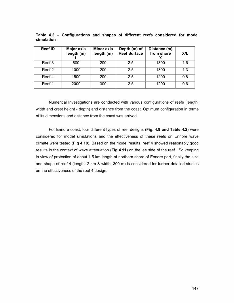
147

Table 4.2 – Configurations and shapes of different reefs considered for model simulation

Reef ID Major axis length (m)

L

Minor axis length (m)

Depth (m) of Reef Surface

Distance (m) from shore

X

X/L

Reef 3 800 200 2.5 1300 1.6

Reef 2 1000 200 2.5 1300 1.3

Reef 4 1500 200 2.5 1200 0.8

Reef 1 2000 300 2.5 1200 0.6

Numerical Investigations are conducted with various configurations of reefs (length,

width and crest height - depth) and distance from the coast. Optimum configuration in terms

of its dimensions and distance from the coast was arrived.

For Ennore coast, four different types of reef designs (Fig. 4.9 and Table 4.2) were

considered for model simulations and the effectiveness of these reefs on Ennore wave

climate were tested (Fig 4.10). Based on the model results, reef 4 showed reasonably good

results in the context of wave attenuation (Fig 4.11) on the lee side of the reef. So keeping

in view of protection of about 1.5 km length of northern shore of Ennore port, finally the size

and shape of reef 4 (length: 2 km & width: 300 m) is considered for further detailed studies

on the effectiveness of the reef 4 design.

148

Fig 4.10a – Reef effectiveness under SE waves

149

Fig 4.10b – Reef effectiveness under SE waves

150

Fig 4.10c – Reef effectiveness under SE waves

151

Fig 4.11 – Reef effectiveness under different configurations

152

The results indicate that reefs reduces wave energy upto 20 to 40% on nearcoast,

there by helps in accumulation of sediments due to reduction in wave intensity. The cross

impacts of these reefs is also minimum when compared to other options. The reef

breakwater was tested with varied crest elevation (depth of water) and simulated wave

height distribution on leeside of reef breakwater is shown in Fig 4.12. Maximum reduction in

wave height is observed when the depth above shoal is 2.5 m.

154

Fig. 4.12 - Configuration of reef breakwater and wave height distribution along the transect taken across the reef

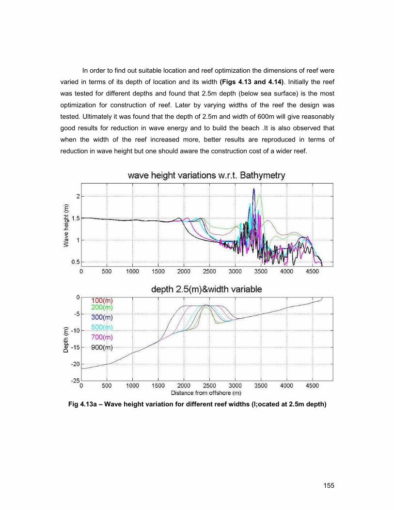
155

In order to find out suitable location and reef optimization the dimensions of reef were

varied in terms of its depth of location and its width (Figs 4.13 and 4.14). Initially the reef

was tested for different depths and found that 2.5m depth (below sea surface) is the most

optimization for construction of reef. Later by varying widths of the reef the design was

tested. Ultimately it was found that the depth of 2.5m and width of 600m will give reasonably

good results for reduction in wave energy and to build the beach .It is also observed that

when the width of the reef increased more, better results are reproduced in terms of

reduction in wave height but one should aware the construction cost of a wider reef.

Fig 4.13a – Wave height variation for different reef widths (l;ocated at 2.5m depth)

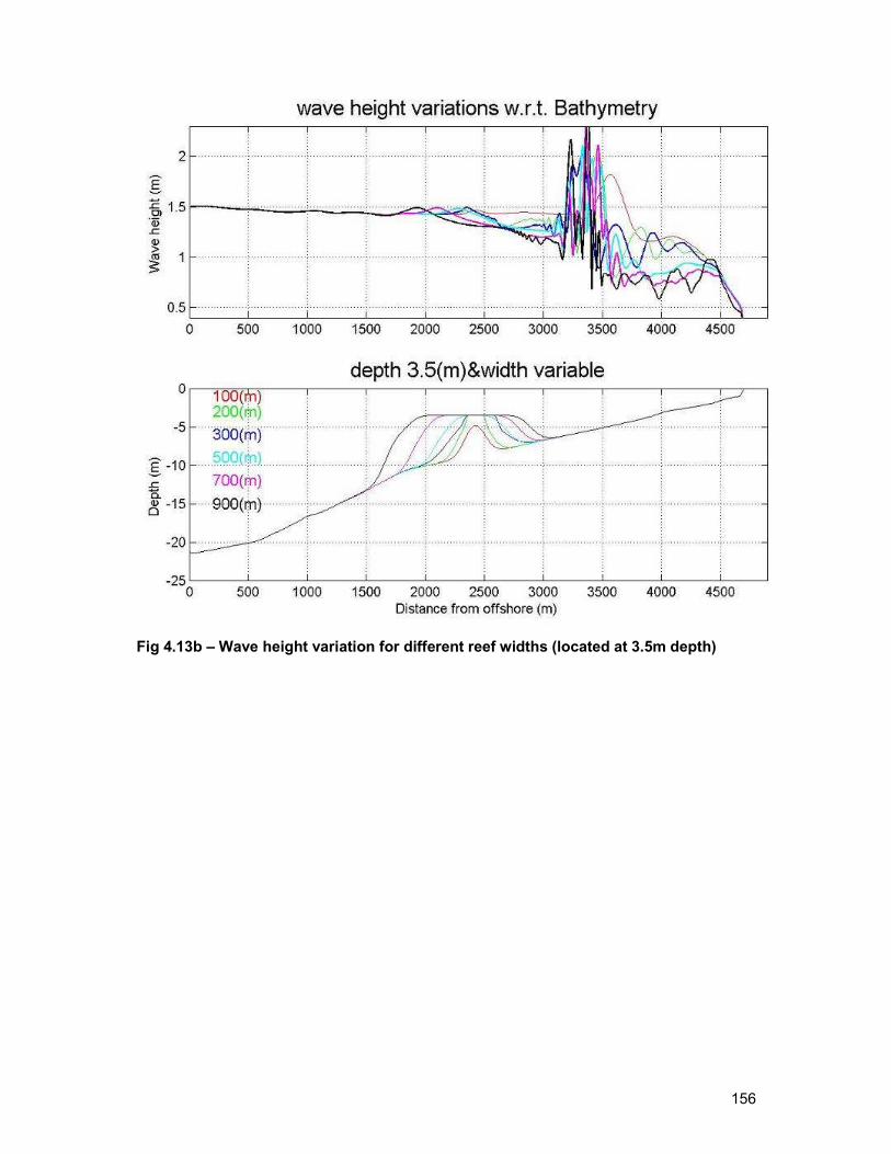
156

Fig 4.13b – Wave height variation for different reef widths (located at 3.5m depth)

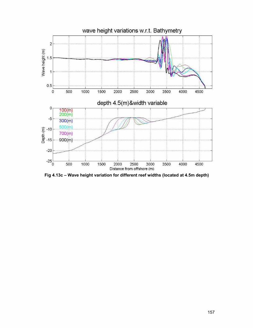
157

Fig 4.13c – Wave height variation for different reef widths (located at 4.5m depth)

158

Fig 4.13d – Wave height variation for different reef widths (located at 5.0m depth)

159

Fig 4.14a – Wave height variation for different reef depths (of constant width 100m)

160

Fig 4.14b – Wave height variation for different reef depths (of constant width 200m)

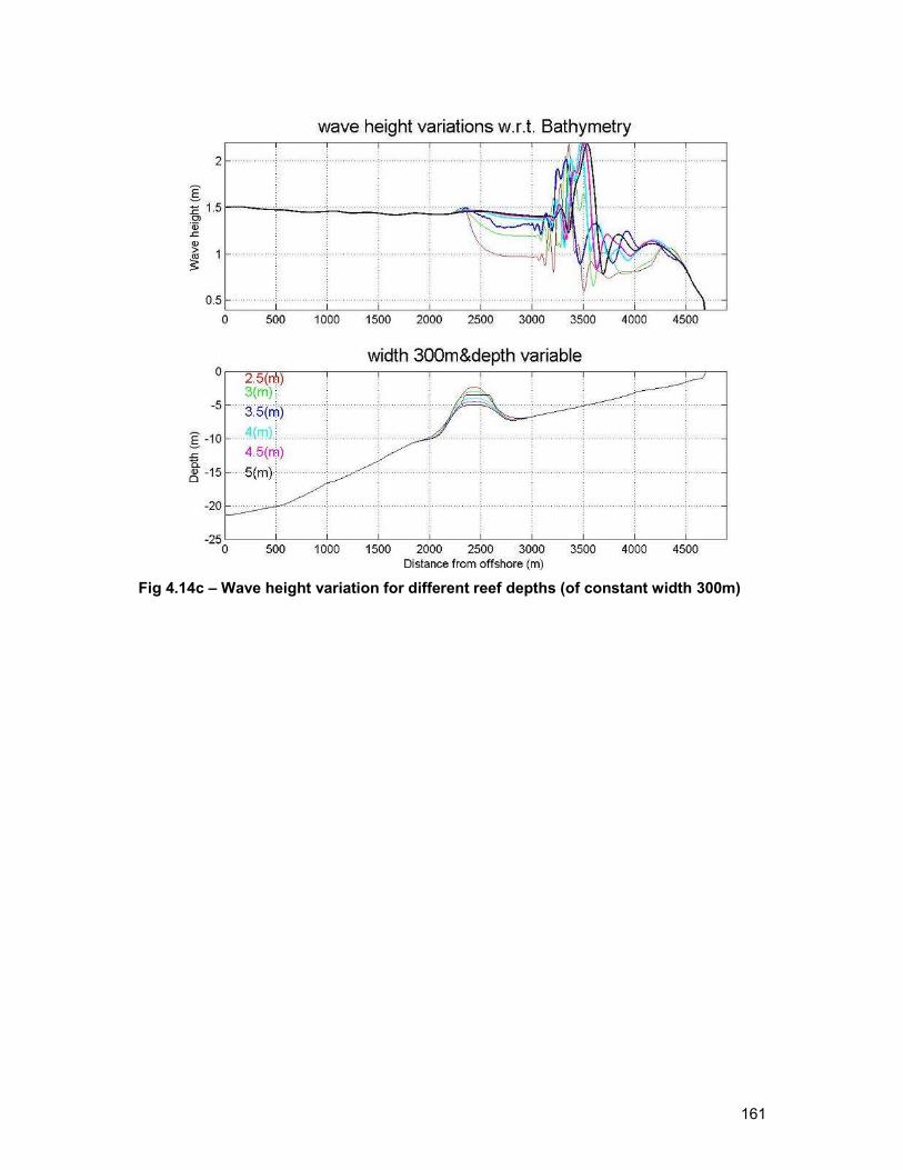
161

Fig 4.14c – Wave height variation for different reef depths (of constant width 300m)

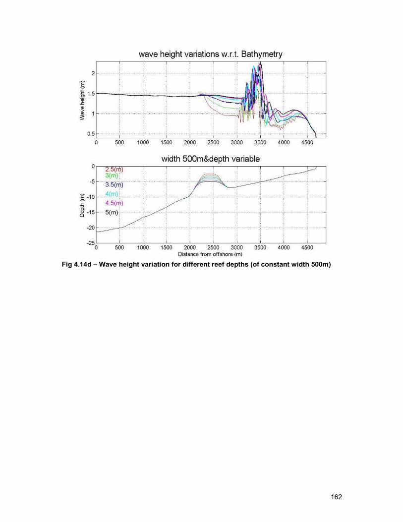
162

Fig 4.14d – Wave height variation for different reef depths (of constant width 500m)

163

Fig 4.14e – Wave height variation for different reef depths (of constant width 700m)

164

Fig 4.14f – Wave height variation for different reef depths (of constant width 900m)

5. RECOMMENDATIONS

The information on hydrodynamic (Tide, wave, current) conditions, shoreline changes

and sediment characteristics was used to estimate sediment budget for the coastal stretch

from Chennai port to Pulicat mouth. Analysis brings out following inferences.

• Sediment is bypassed to north at Chennai port through south breakwater.

Construction of groin field at two coastal stretches along Royapuram coast has

blocked part of sediment during year 2004-2005. Recent observations indicate that

the accretion was reduced.

• The Beach, south of the port, is accreting at a rate of 45 m per annum, extended

offshore 320 m, and alongshore 2.6 km, causing increased siltation in Ennore Creek.

On north of port, 600 m length of beach fill is eroding at the rate of 50 m and the zone

of erosion is shifting further north. During 2003 - 2004, the erosion length was

165

extended up to 1500 m and 100-m width of beach was lost outside the nourishment

area. Coastline adjacent to beach fill underwent readjustment and a village Katuppali

located 2.5 km from the north breakwater is experiencing erosion to an order of 30 m

per year.

• Predictions made using numerical model indicated that beach fill placed by port

authorities would be completely lost to sea by 2007 and original coast will be under

threat if no intervention is planned.

Four interventions are worked out based on the field investigations and numerical

experiments – Artificial beach nourishment, Sand bypassing, Groins/Offshore breakwaters

and Offshore submerged reefs. The advantages and limitations of each intervention are

discussed below.

• Artificial beach nourishment, which was implemented by port authorities by dumping

3.5x106 m3 of sand obtained from capital dredging performed well in controlling the

erosion on northern side by way of supplying sediments to north. The detailed

analysis made from the beach profiles and numerical modeling indicates that life of

the project can be increased by arriving suitable dimensions of beachfill and

transition length. Beachfill with a of length 1000 m, width 600 m with a transition

length of 800 m would result in increase in the life of the project by one more year

and the impact on adjacent coast can also be minimized.

• Sand bypassing is also proven to be better option for coastal protection along east

coast of India, but requires periodic maintenance of equipment like pumps and pipes.

Alternatively disposing of sand dredged from maintenance dredging to north of port

through rainbow disposal, which is being currently implemented in Visakhapatanam

port. The annual maintenance dredging expected at Ennore port would be around

0.3 x106 to 0.5x106 m3.

• Though option of groin field was worked out, it may not be efficient at Ennore port, as

the sediment supply to north of port is limited by configuration of entrance channel.

Observations indicate that coarser sediments coming from south are trapped into

entrance channel of Ennore port. As a result, the finer sediments are only bypassed

to north as suspended load, which may not be useful in building the beach.

Construction of groins will also result in erosion of the coastal stretch further north of

groin field.

166

• Offshore submerged reefs are one of the soft option which is implemented in New

Zeeland, Australia and US and results of this option was more environmentally

friendly and adaptive. Numerical Investigations are conducted with various

configurations of reefs (length, width and crest height) and distance from the coast.

Optimum configuration in terms of its dimensions and distance from the coast was

arrived. The results indicate that reefs reduces wave energy upto 20 to 30% on

nearcoast, there by helps in accumulation of sediments due to reduction in wave

intensity. The cross impacts of these reefs is also minimum when compared to other

options.

167

6. REFERENCES

ASR (2000) Ltd. Marine and Freshwater Consultants Report,P.O. Box 67, Raglan, New

Zealand. Tel: +64 7 825 0380, Fax: +64 7 825 0386 E-mail: enquiries@asrltd.co.nz. Web:

www.asrltd.co.nz

Balsillie J H and Berg DW 1972. State of groin design and effectiveness. Proceedings 13th

International Conference on Coastal Engineering, 1367-1383

Basco, D. R., and J. Pope, 2004. Groin Functional Design Guidance from the Coastal

Engineering Manual. Special Issue 33, Journal of Coastal Research, 121- 130.

Black, K. P., 2000. Artificial surfing reefs for erosion control and amenity: theory and

application. International Coastal Symposium (ICS2000) Invited paper. Rotorua, April, 2000.

Black, K., 2001, Artificial Surfing Reefs for Erosion Control and Amenity: Theory and

application, Journal of Coastal Research, 1-7 (ICS 2000 Proceedings), New Zealand; (see

also ASR Ltd, Marine & Freshwater Consultants, PO Box 151, Raglan, New Zealand,

k.black@asrltd.co.nz; www.asrltd.co.nz).

Black, K. P., and C. Andrews, 2001a. Sandy Shoreline Response to Offshore obstacles

Part 1: Salient and Tombolo Geometry and Shape. Journal of Coastal Research, Special

Issue 29: 82-93.

Black, K. P., and C. Andrews, 2001b. Sandy Shoreline Response to Offshore obstacles

Part 2: Discussion of Formative Mechanisms. Journal of Coastal Research, Special Issue

29: 94-101.

Bramption, A.H., Powell, K.A., Goldberg D.G., and Lowe J.P., 1991. Application of

numerical and physical modeling to beach management problems. COPEDEC III

conference., pp 1.15

Capobianco, M., Hanson, H., Larson, M., Steetzel, H., Stive, M.J.F., Chatelus, Y., Aarnin

Khofs., and Karambas, T., 2002. Nourishment design and evaluation: applicability of model

concepts, Coastal Engineering 47 (1), 113-135.

Chandramohan, P., Nayak, B.U. and Raju, V.S. (1990) Longshore-transport model for

south Indian and Sri Lankan coasts. ASCE Journal of Waterway, Port, Coastal and Ocean

Engineering 116, 408-424.

Coastal Engineering Research Center (CERC), 1984 Shore, Coastal Engineering

Research Center, Army Corps of Engineers, Virginia, Vol I and II.

Folk R.L and Ward M.C (1957). Brazos river bars: A study in the significance of grain size

and mineral composition in sedimentary rock nomenclature, J Geol., Vol 62, pp 344-359

Hanson, H and Kraus, N.C., 1993. Optimization of beachfill transitions, Beach nourishment

Engineering and Management considerations. In: STAUBLE, D.K and KRAUS, N.C (eds.),

Proc. Coastal Zone ’93 ASCE, pp. 103-117.

168

Inman D.L (1949), Sorting of sediments in the light of fluid mechanics, J Sed. Petrol., Vol 19,

pp 10-30.

Kaliasundaram G., Govindasamy S and Ganesan R (1991), Coastal erosions and

accretions. In: Coastal zone Management in Tamilnadu state, India ((Natarajan R., Dwivedi

S N and Ramachandran S eds), Ocean Data Center, Anna University. Madras pp 73-82

Kraus, N.C., 1995. The use of structures to hold beachfill: An overview, Proc. 8th National

Conference on Beach Preservation Technology, Florida Shore & Beach preservation

Association, (Tallahassee, Florida).

Leatherman, S.P., 1991. Coasts and Beaches, In: Kiersch, G.A (ed.), The Heritage of

Engineering Geology, The First Hundred Years. Boulder, Colorado: Geological Society of

America Special Volume 3, pp 183-200.

Mani, J.S (2001) Protectve measures for Ennore creek in Madras. A numerical approach, In:

Quaternery sea-level variation, shoreliene displacement and coastal environment. Victor

Rajamanickam and Michael Tooley (eds), New Academic Publication, pp 230-235.

Mead, S. T., K. P. Black and P. McComb, 2001. Westshore Coastal Process Investigation. Technical report for Napier City Council, September 2001. Mead, S. T., K. P. Black, C. Blenkinsopp and P. McComb, 2003c. Reef Design and Physical Processes. For the Lyall Bay Surfing Reef Charitable Trust, Wellington, March 2003.

Piorewicz, J., 2002. Proceedings of the Public Workshop – Yeppoon 2002. Ed. J. Piorewicz, Central Queensland University Press.

Pratt, J. R., 1994. Artificial habitat technology and ecosystem restoration: managing for the

future. Bulletin of Marine Science 55(2-3), 268- 275.

Shankar D., McCreary J.P., Han W and Shetye S.R (1996), Dynamics of the East India

Coastal Current: Analytic solutions forced by interior Ekman pumping and local alongshore

winds’, J Geophysical Research, Vol 101, No 13, 975-13, 991

Turner D.D (1994), Sediment transport on an estuarine beach: a comparision of different

methods, unpublished masters thesis, dept of Oceanography, Univ Southampton, p 120.

US Army Corps of Engineers, 1995. Design of Coastal Revetments, Seawalls, and

Bulkheads. Department of the Army, US Army Corps of Engineers, Washington DC 20314-

1000.

US Army Corps of Engineers (USACE), 2001. Coastal engineering manual 1110-2-1100,

U.S Army Corps of Engineers, Washington, D.C

Wentworth C.K (1947) A laboratory and field study of cobble abrasion, J Geology, Vol 27,

pp 507-521

169

.