These slides are from a presentation that I gave to the Oregon chapters of the ASCE General Section/Geotechnical Group Dinner Meeting on May 6, 2015. This presentation evolved (devolved?) mostly into a description of my experience in development and application of methods for assessing landslide hazards over the past 20 years. I gathered slides and figures from presentations and papers over thattime. I’ll add notes for these slides, to make them slightly more interpretable, and post them to the TerrainWorks website. Please feel free to use anything here.

1

Risk is defined in terms of the hazards posed by landslides together with the consequences of landslide occurrence. How we define risk thus depends on how we measure hazard and on how we value the resources affected by landsliding at any particular site.Hazard is defined in terms of the locations affected by landslide processes, the frequency with which landslides occur, and the magnitude of landslide effects. For this presentation, I’ll be focusing on where landslides tend to occur and areas directly affected by landslides from upslope – on measures of susceptibility.

2

My history provides context for what I have to say. I come with a numerical background, so I tend to tackle problems by writing computer programs, primarily in Fortran, for data analysis and for forward and inverse modeling of physical processes. After moving to the Pacific Northwest in 1987, my wife (Lynne, who is also a geologist) and I were involved in several hazard-assessment efforts in Washington state: the development and implementation of the Watershed Analysis program, mapping of slope-stability hazards for the Critical Areas Ordinance, and in geotechnical reviews for forest practice applications. These experiences motivated my post-graduation research efforts, starting with a post-doctoral position at UW, then with the founding of the nonprofit ESI in 1997 with Lee Benda, and continuing last year as Lee and I started TerrainWorks, a for-profit company whose mission is to find sustainable revenue sources to support the tools developed through the research that we and other scientists have done.

3

4

I’ve used this slide in most of my talks over the past two decades. For geomorphologists, this is one conceptual construct from which we seek to interpret what we see. Below are the notes from another talk, focused on fish habitat. It may seem strange that study of fish leads to a need to understand landslides, yet in mountainous environments, landslides are key components of habitat formation, and it is funding for habitat-focused projects that supported most of this research.

Habitat attributes arise from process interactions over multiple scales. To find the underlying controls on the spatial and temporal distribution of habitat types requires a perspective that encompasses multiple scales. This allows one to see how events distant in space and time act to create channel conditions encountered at some specific point here and now. It is useful conceptually to simplify this complex system by separating the factors involved into four broad categories: 1) An approximately static, but heterogeneous spatial template, created by basin and valley

topography, that determines where sediment is produced, where it enters the channel system, and where it will be stored along the valley floor.

2) Temporally dynamic drivers that act to alter erosional susceptibility and to trigger erosional and sediment transport events (landslides, floods).

3) A branched and hierarchical channel network through which sediment and organic debris is moved intermittently through and eventually out of a basin. Erosional events supply pulses of sediment that are modified and interact as they are moved downstream through the network. Channel confluences juxtapose different and potentially independent sediment transport regimes at tributary junctions.

4) A history of events that determines the spatial distribution of vegetation and the volume of material available for erosion and storage.

These factors are of course inter-related; separating them conceptually allows us to examine and characterize the parts independently and then to look at interactions between each component.This talk focuses on aspects of the Spatial Template, but all four must be considered to fully characterize watershed interactions.

A key event for me in development of landslide assessment methodologies was a decision to build simulation models of sediment and woody debris fluxes over entire watersheds for periods spanning thousands of years. I worked on this with Lee Benda in the mid 1990s. There were no off-the-shelf tools, so we developed and coded all of this ourselves. This forced us to think through, in careful detail, all the factors involved with sediment and wood production and transport. We knew, from extensive field work (ours and many others) that landslides were a primary mode of transport from hillslopes to valley floors. We used extensive landslide inventories with C14 dating from headscarps and deposits to constrain frequency of occurrence for different processes, and calibrated the models against these frequency distributions.

5

Animations created using these simulations were used with field photography in a series of instructional videos produced with the Forest Service in 2002. These videos, with other documentation, are available on the TerrainWorks website (terrainworks.com/landscape-dynamics).

6

Landslide hazards were not our focus, but to characterize sediment fluxes, we had to deal with all the factors that determine hazard. To do so, we used detailed information about the spatial and temporal distribution of soils, pore pressures, and effective root cohesion from forest stands, all obtained from linked spatially and temporally distributed physical models for these processes.

7

Not long after starting Earth Systems Institute, we started collaborating with the Coastal Landscape Analysis and Modeling Study.

8

Our involvement was with development of broad-scale models. We had written the software for characterizing controls on landslide initiation and debris-flow runout, but we did not have sufficient data to run process-based models over the entire Oregon Coast Range. So we chose instead to look for empirical correlations between observed landslide locations and runout extent with those physical characteristics that the process-based understanding suggested should pose primary controls on landslide processes.

9

10

Ultimately, the goal was to provide GIS-based tools to assess landslide susceptibility and the effects of land management on susceptibility.

We had two extraordinary data sets to work with: a field-based landslide inventory and a photo-based inventory spanning a large portion of the Coast Range, both for landslides triggered by large storms in 1996.

11

For shallow-rapid landslides, the type that trigger debris-flows in the Coast Range, we figured that topography, geology, and land cover are the primary controls on where landslides initiate. To separate the role of topography, we looked at how landslide density varied with different topographic locations in the landscape. Topographic location was characterized in terms of a topographic index, which incorporates the topographic attributes that affect landslide initiation. These attributes differ for different landslide types. For failure of shallow soils overlying lower-permeability substrates, we used an index that incorporated gradient, curvature, and total or partial contributing area. We looked at how observed landslide density varied as a function of the topographic index. For this analysis, we assumed that the effect of topography was the same under different conditions of landcover, geology, and precipitation – assumptions I’m working now to eliminate.

12

Having a relationship between topography and landslide density allowed us to createmaps of relative landslide density using only digital elevation data. These provide one way to characterize landslide susceptibility: we expect more landslides to occur in zones of high density and fewer in zones of low density.

13

We have an index value for every DEM cell and for every mapped landslide initiation point. By ranking the topographic index from highest to lowest landslide density, and then plotting the proportion of the DEM area against the proportion of mapped landslides for each index value, we can compare the performance of different indices, or different models of landslide susceptibility. You can think of this as identifying the index (model) with the fewest false positives, in that it minimizes the area with no landslides mapped with higher landslide densities. In this plot, Shalstab refers to the process-based model described by Montgomery and Dietrich, 1994, Water Resources Research, 30:1153-1171; slope refers to surface gradient, and slope+convergence refers to a function of surface gradient and plan curvature. For this landslide inventory, collected from aerial photographs spanning a 40-year time period over portions of the Cowlitz Basin, the slope+convergence index performs best.

These curves provide another way to assess susceptibility to landslide initiation. Each point along any curve corresponds to a specific topographic index value. To identify those areas that contain a given proportion of all mapped landslides, we simply chose a proportion and find the corresponding index value. These curves show what proportion of the DEM area has index values with associated landslide densities

14

greater than or equal to that of the chosen index value.

14

Here is an example of susceptibility to landslide initiation mapped in terms of the proportion of mapped landslides contained within a given zone for an area at the north end of Hood Canal in Washington. We expect that the same areas will contain the same proportion of future landslide events. This is a testable prediction.

15

16

Having characterized the effects of topography, we then sought to characterize the influence of other factors on landslide density, in particular, effects of land cover.

17

Here are measured landslide densities under different forest-cover types

obtained from the Siuslaw National Forest landslide inventory. This is the usual

story: highest landslide densities in clear cuts, lower densities in progressively

older forest stands. In the histogram, “Uncorrected” refers to the raw data;

“Photo Bias Corrected” refers to densities corrected for the bias inherent in

landslide mapping from aerial photographs (small landslides are not visible

under forest canopy); and “Bias and Topo Corrected” refers to density values

corrected for both detection bias and differences in topography for different

cover types. For example, roads tend to be located on flatter terrain

(topography with intrinsically lower landslide density), so the calculated density

needed to be adjusted upward to compare directly with the other cover types.

Large Conifer stands tended to be located on steeper terrain than average

(i.e., higher intrinsic landslide density), so that density value needed to be

adjusted downward for comparison with other cover types. These methods are

described in Miller and Burnett, 2007, Water Resources Research,

43:W033433.

Here is an example from a more recent study, looking at landslides associated with a large storm in SW Washington in 2007. Here too, landslide density was found to correlate with topographic attributes (surface gradient) and land cover (stand age). Precipitation data were also available for this study: landslide density was found to depend strongly on storm characteristics. In the histograms, the white portion of the bars shows the correction for detection bias from air-photo landslide inventories. The vertical lines show confidence intervals on those corrections.

18

Given the problems with detection bias, it would seem that we should focus our efforts on field surveys that attempt to obtain a complete census of landslide events. Here are examples of landslide densities associated with different stand types from field surveys conducted in the Oregon Coast Range after the 1996 storms and in SW Washington after the 2007 storm. Relationships are not so clear: the decrease in landslide density with increasing stand age found in the photo-based inventories is not always replicated with field studies.

19

20

In fact, we find the same behavior in the photo-based inventories. Here we

randomly placed circles of varying radius on the study area and calculated

landslide density for each cover type. The mean landslide density within each

circle varied widely when the total area of the circle was small, and the

variability decreased as the area increased, converging on the mean landslide

density for the entire study area. Here we had two separate areas, so we see

convergence to two different mean values. Field-based inventories typically

encompass about 10 square kilometers.

The diagonal lines of points in the scatter plot correspond to circles containing

one landslide (the lowest line), two landslides, and so on.

21

When we compared landslide densities for different forest types within a single sampled area, we found something interesting. For small sample areas, a few tens of square kilometers or less, many samples had a higher landslide density in the LARGE cover type than in the OPEN or MIXED, opposite the results shown in Slide 17, but consistent with the Elk Creek, Mapleton, and Vida field sites shown in Slide 19. The proportion of samples for which this was true (density LARGE > density MIXED or OPEN) decreased as the size of the sample area increased, until at about 400 square kilometers all samples had higher densities in the OPEN category and at about 1000 square kilometers all samples had higher densities in the MIXED category. There are a variety of possible explanations, but my point here is that it is important to keep an open mind when evaluating study results. There can be more than one right answer, none of which may be the right answer for your particular question.

Landslide initiation is only half of the story; we still need to characterize susceptibility to effects from debris-flows triggered by landslides from upslope. We took an empirical approach for this as well. Field observations show that debris flows tend to erode material and increase in volume as they travel through steep, confined channels and to deposit material and decrease in volume as they traverse lower gradient and less confined zones, like fans. We used field-surveys to identify zones of scour and deposition along recent debris flow tracks. These observations can be used to create field-based criteria for estimating debris-flow travel extent (if the field surveys include measures of channel gradient and valley width), but our interest was in using digital data to map debris flow susceptibility over entire watersheds, so we overlaid the field surveys on digital elevation data and used DEM-estimated surface gradient and channel confinement to characterize zones of scour and deposition. We characterized these zones in terms of the proportion of surveyed sites exhibiting scour or deposition as functions of Sw, where Sw is a measure of channel gradient and confinement.

22

Observed relationships are affected by forest cover. For a given Sw value, debris flows through forested zones are more likely to deposit rather than scour. Likewise, we find that these relationships are affected by underlying geology.

23

To estimate probably runout extent, we used the simple fact that a debris-flow terminus indicates the point where the volume eroded equals the volume deposited. We used the probability of scour (as a function of Sw), integrated along the travel path, as an indicator of total volume eroded. We used probability of deposition, integrated along the travel path, as an indicator of total volume deposited. For mapped debris flows, we plotted a cumulative distribution of the ratio of these integrated values. This cumulative distribution provides an empirical estimate of the probable runout extent for a debris flow originating from any point as a function of the slope and topographic confinement along the travel path. Starting from any point, we can follow the flow path downslope and calculate PS and PD values from the DEM, integrate these along the flow path, calculate the ratio, and use the cumulative distribution to see what proportion of observed debris flows stopped at that ratio value.

24

By then integrating over all potential upslope debris flow sources (all DEM cells with an estimated landslide density greater than zero), we can calculate a conditional probability that a debris flow was mapped in any point in the channel network. This probability depends on the number of upslope sources, the estimated landslide density of each upslope source, and the probability of delivery from each source, which depends on the slope and channel confinement along the travel path from each source.

25

We now have all the pieces to calculate an empirical susceptibility to direct debris flow impacts, including impacts from both scour and deposition.

Debris-flow impacts, however, depend also on what the debris flow encounters along its runout path. Debris-flow effects on streams depend very much on how much large woody debris (large standing and fallen trees) is encountered enroute and ends up in the debris-flow deposit. To reduce risk posed by debris flows for aquatic habitat, we want to ensure that there are large standing and fallen trees available for future debris flows to pick up. For that, we wanted to identify those headwater channels most likely to be traversed by a debris flow that continued downslope to a fish-bearing stream.

The first step is the probability of landslide initiation. We estimate this probability using landslide density. If the landslides in an inventory represent all landslide events over a given period of time, we can interpret density as a rate and use a Poisson distribution to estimate the probability for landslide occurrence within any given area, e.g., a DEM cell, over a specified time. If we don’t know the time period represented by landslides in an inventory, we can use the same approach but interpret the probability in relative terms.

26

For each DEM cell with a landslide density greater than zero, we then calculate the probability that a debris flow originating in that cell will travel to any point downslope. We can than ask, what is the probability that any point along a headwater channel network will be traversed by a debris flow from upslope that continues to a fish-bearing stream downslope.

27

We make this calculation for all upslope cells, and calculate a conditional probability that one or more of those upslope cells contains a mapped landslide that triggered a debris flow that traversed the point of interest and continued to a fish-bearing channel downslope.

28

This would take a very long time without a computer. There is a persistent belief among many geologists that landslide hazards can be assessed only with field observations. That is true, but field observations alone are insufficient to quantify hazard. You have to integrate the potential for landslide initiation and runout from every upslope point.

29

These methods allow translation of field observations and photo surveys to regionalcalculation of susceptibility to debris flow impacts. We can define “impacts” in a variety of ways: susceptibility for initiation, susceptibility for traversal from a debris flow from upslope, susceptibility for traversal from a debris flow from upslope that continues to a fish-bearing stream.

30

Recall how we characterized susceptibility to landslide initiation by mapping the area that encompasses a specified proportion of observed landslides. We can take the same approach with runout: identify those debris-flow corridors that include a specified proportion of all mapped debris-flow runout tracks, starting with those having the highest susceptibility to debris-flow traversal.

If we want to leave buffers on debris-flow-prone channels to ensure future wood recruitment to fish-bearing streams by debris flows, we can choose what proportion of the debris-flow track length to protect.

31

32

33

Here is an example from Knowles Creek, in the Oregon Coast Range.

34

Debris flows don’t just affect stream habitat. Five people were killed by debris flows in Oregon in November, 1996, motivating passage of Oregon Senate Bill 12 in 1999, which aimed to identify and reduce hazards posed by debris flows. Jon Hofmeisterand I adapted the empirical methods described in the previous slides and implemented methodology to identify debris-flow inundation zones. These were used to map potential debris-flow hazards across Western Oregon. The methods we developed are described in the IMS-22 report and in Hofmeister & Miller, GIS-based Modeling of debris-flow initiation, transport and deposition zones for regional hazard assessments in western Oregon, USA, in Debris-Flow Hazards Mitigation: Mechanics, Prediction, and Assessment, 2003, Reickenmann and Chen (eds), Millpress, Rotterdam, p.1141-1149.

35

The hazard maps produced for IMS-22 were based on 10-m DEMs derived from contour lines on 1:24,000-scale topographic maps. The hazard maps are available at http://www.oregongeology.org/sub/publications/IMS/ims-022/ims-022.htm, with the above disclaimer. Similar caveats were given in the original IMS-22 report, but with the advent of LiDAR DEMs much better elevation data are now available. However, I’m interested in how wrong the original maps are. Most of the world doesn’t have high-resolution LiDAR DEMs. How much can we learn with the data we have?

36

Enough of the easy stuff; on to deep-seated landslides. Even as we worked on the debris-flow studies, we were quite aware of the ubiquitous presence of these large landslides. This is a photo and field-based inventory from southwest Washington, including the Tilton Basin where Lee Benda and I created our simulation model. Over 40% of the surface area is mapped as some sort of landslide feature. So we know they’re there, we just don’t know what hazards they pose. Most show no evidence of recent activity.

37

Here’s another inventory of large landslides, for a portion of the North Fork Stillaguamish River valley, mapped on LiDAR shaded relief imagery. Deep-seated landslides line the valley walls. In fact, it was landslides in this area that motivated my post-doctoral work on deep-seated landslide hazards.

The Oso landslide is number BA 4N.

38

So we knew these landslide features were out there, we knew they posed potential hazards: we just didn’t know which sites posed a hazard or how things we did might alter those hazards, by for instance destabilizing a currently dormant landslide.

39

We did not have information on a large population of landslide events with which to build empirical models, as we had for shallow-rapid landslides and debris flows, so I went back to a process-based strategy. We used a plane-strain, limit-equilibrium approach. Available DEMs provided surface topography; available geologic mapping provided an estimate of stratigraphy; we could map existing landslide features from photo stereo pairs; we used published ranges of material properties (bulk density, friction angle, cohesion) and back calculated to a factor-of-safety near 1.0 for existing landslide features and greater than 1.0 for slopes without mapped landslides to set final values.

We generated transects from every DEM pixel aligned with slope aspect and extending from ridge top to valley floor. Along each transect, we generated slip surfaces between every combination of points along the transect profile (sampled at the DEM point spacing). For each combination of points, we found the tension-crack depth and radius of curvature (assuming circular slip surfaces, with radius somewhere between infinity – a wedge – to half the distance between the two slip-surface endpoints) that gave the minimum factor of safety. For every DEM cell along the transect, we tracked the minimum factor of safety of any slip surface that crossed it. We generated transects from every DEM cell to create a map of minimum factor of

40

safety.

40

Not that we trusted those factor-of-safety values. Rather, we were interested in how the calculated factor of safety would respond to a perturbation in topography or pore pressure. We were looking for where the topography and stratigraphy inferred from geologic mapping indicated slopes sensitive to changes. And it was this methodology that eventually brought me to what was known back in the 1990s as the “Hazel” landslide.

41

Perhaps this view looks familiar. This is the North Fork Stillaguamish valley looking east, with the Oso landslide on the north side – as it looked in 2006.

42

This is the title slide from a powerpoint presentation I made in 2006, after activity on the landslide had blocked the river in January. This site had a history of activity, and it was that history that motivated studies to better understand what factors affected landslide behavior.

43

These are some of the questions being asked in the mid 1990s about deep-seated landslides in general, and about the Hazel landslide in particular. These were (are) challenging questions, and the methods we had to answer them were not really up to the task. In the end, decisions were based entirely on professional judgement.

44

So I argued that it would be worthwhile to try something different and take a modeling approach.

45

I had the plane-strain, limit-equilibrium approach described previously ready to go. We needed methods to estimate changes in groundwater recharge, for delineating the groundwater recharge zone, and for determining pore pressures and effects on landslide behavior.

I worked with Joan Sias, a graduate student in civil engineering. She developed a model to estimate evapotranspiration rates for the Hazel site under different forest stand scenarios. We used a 2-D finite element groundwater model (MODFE, http://water.usgs.gov/software/MODFE/ ) developed by the USGS, which I modified to account for temporally and spatially variable surface seeps. We coupled all these models together, derived precipitation, wind, temperature, and humidity time series to drive the models from the weather-station data, and looked to see what this modeling approach suggested about landslide response to different environmental factors.

46

We estimated stratigraphic relationships by extrapolating contacts mapped at the surface. We generally inferred the contact between the permeable glacial outwash and underlying lake-bed (lacustrine) sediments by the presence of surface seeps. The surface and subsurface geometry are largely determined by past movement of large landslide blocks; we approximated sub-surface geometry of the outwash-lacustrine contact by vertically lowering the contact within each block to the elevation of the observed surface seeps. We then treated the advance outwash as an unconfined aquifer.

It turns out that we missed an important component of the stratigraphy: there is a layer of till overlying the advance outwash, with recessional outwash overlying the till. In the mid 1990s, when we did the field work, we did not see any till exposed in the headscarps and missed exposures on the steep, soil-covered slopes. After the 2014 event, the till is readily seen in the headscarp. However, locations of seepage observed in the 90s appear to be associated with the advance outwash – lacustrine contact, not the recessional outwash-till contact.

47

For a given forest-cover scenario, the evapotranspiration and ground-water models provided a spatially and temporally varying water table surface. We used this, with the inferred stratigraphy, for calculating factors of safety along transects, as described in slide 40. With these models, we examined several issues: sensitivity of calculated factors of safety associated with changes in ground-water recharge caused by removal of forest cover, sensitivity to changes in slope geometry caused by erosion by the Stillaguamish River, and sensitivity to changes in slope geometry caused by incision of streams draining the body of the landslide.

48

I didn’t have the computing power (we did this all on a 1990s vintage PC) to run full spatially and temporally explicit scenarios, so we used steady-state analyses to examine sensitivity, with groundwater recharge at each grid cell set to the temporally averaged mean value for each scenario. We looked at the difference in calculated minimum factors of safety for all DEM grid cells for forested and unforestedconditions. Joan Sias provided a range of recharge time series, reflecting the range of uncertainty in parameters used in the evapotranspiration model. This slide shows the proportional change in calculated factor of safety, for all grid cells with a minimum value of 1.3 or less, for the set of parameter values that produced the smallest change in groundwater recharge between the forested and unforested cases.

49

This slide shows the proportional change for the set of parameters that produced the largest difference in groundwater recharge between the forested and unforestedconditions.

50

We wanted to compare the relative importance of different processes affecting the landslide, and see which areas of the landslide were potentially affected by different processes. This slide shows the proportional change in calculated factor of safety associated with erosion of the toe of the slope by the Stillaguamish River. One calculation was made for the topography in 1978 (the photo year the contour map was created from); the other made by placing the river at its current position at the time of the study. As expected, there is a large reduction in factor of safety at the toe of the slope. It is informative to see, however, that this reduction is more than twice that associated with changes in ground water recharge from timber harvest (compare the legends in slides 49 and 50).

51

Field observations also indicated that surface geometry of the landslide body was altered by incision and bank slumping of channels that drained surface seeps. Modeled changes in stability associated with incision of those channels indicated sensitivity in locations of observed landslide activity. Again, note the scale in the legend.

So what’s the point of all this? The goal is to provide information to guide management decisions. In this case: is it OK to cut timber upslope of the landslide? The models don’t provide the answer, but can provide insight to those responsible for making a decision. As it turns out, additional “information” may seem to make the decision making more complex, and introduces more questions, such as “how much do we trust model results?”

We used all available information to infer specific slope locations where the landslide would respond to different environmental changes (increased groundwater recharge associated with reduced evapotranspiration from timber harvest, cutting of the slope toe by the Stillaguamish River, erosion of channels draining the landslide body) and provided estimates of the relative reduction in stability associated with each. But we have no way to directly measure “factor of safety”; indeed, “factor of safety” is a

52

conceptual construct that relates to how we expect the landslide to behave.

So one test of the models is to watch landslide behavior, see how it actually does respond to environmental changes, and compare to model results. The brown lines indicate areas of landslide activity observed in 1991 photographs. How do these areas of observed activity compare to locations of modeled high sensitivity? The best matches are with erosion of the slope toe by the Stillaguamish River (slide 51) and to erosion of channels draining the landslide (this slide). Areas modeled as sensitive to changes in groundwater recharge do not correlate well with observed locations of landslide activity.

To further test these models, and to develop “better” models, requires more information. Installation of monitoring wells or piezometers could have provided information on the actual groundwater flow field, installation of precipitation gauges could have provided information on actual canopy interception.

52

In 1999 I was asked to provide a brief description of the geomorphology of the Hazel and Gold Basin slides to inform planning efforts seeking to reduce fine sediment inputs to the Stillaguamish River from these locations. I used the stability model described previously (slide 48), but modified to provide depth to a slip surface with a specified factor of safety. Shown here are calculated depths for a factor of safety of 1.0.

To estimate the extent of runout were this material to fail, I integrated depths along transect A-A’. A one-meter-wide slice along this transect contained 5425 m3. Field observations here and at other locations within the Stillaguamish Basin showed that debris flow deposits in these glacial sediments tended to form fans with a surface slope of about 15%. A wedge of material with a surface slope of 15% and containing 5425 m3 of material would extend 270 m.

The report is available here: http://www.nws.usace.army.mil/Portals/27/docs/civilworks/projects/Hazel-GoldBasinLandslidesGeomorphicReviewDraft.pdf

53

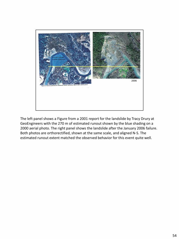
The left panel shows a Figure from a 2001 report for the landslide by Tracy Drury at GeoEngineers with the 270 m of estimated runout shown by the blue shading on a 2000 aerial photo. The right panel shows the landslide after the January 2006 failure. Both photos are orthorectified, shown at the same scale, and aligned N-S. The estimated runout extent matched the observed behavior for this event quite well.

54

Here is another figure from my 1999 report, with the gray scale converted to color. Here the depth to a failure surface with a factor of safety of 1.3 is shown. I had included this figure in the report because activity on the landslide in the late 1990s was altering the surface geometry (see the brown lines on slides 49-52), which I thought would cause my calculations, based on 1978 topography, to over-estimate stability of the landslide so that a factor of safety of 1.0 would under-estimate the volume of material potentially mobilized in a landslide event.

Note that the simple runout model I used – extending the volume of failed material into a wedge with 15% surface slope – would have under predicted runout in the 2014 event. Even if the volumes were of the right order of magnitude, the average surface slope of the deposit was about 6%.

55

So, in the context of deep-seated landslide hazards, does a modeling approach provide any advantages over professional judgement alone, even when we lack subsurface data? Yes, although there is much yet to be learned for using models effectively. There’s no way to avoid professional judgement, and neither should we –professional judgement is involved in building, evaluating, and using models too – but we can use these tools to test and evaluate professional judgement.

56

What’s next? Here’s my list. Data are a key component, and there is a lot of discussion now about “hazard mapping” in terms of data collection – e.g., “we need LiDAR”. But we need to know what to do with the data we collect. Knowing where landslides occur is only the first step in hazard assessment, and we need to quantify hazards in order to assess risk.

57