i'llll i,l ~ll i'.) - home | santa fe...
TRANSCRIPT

Physica D 42 (1990) 153-187 North-Holland
A R O S E T r A STONE FOR CONNECTIONISM
J. Doyne FARMER Complex Systems Group, Theoretical Division, Los Alamos National Laboratory, Los Alamos, NM 87545, USA and Santa Fe Institute, 1120 Canyon Road, Santa Fe NM 87501, USA
The term connectionism is usually applied to neural networks. There are, however, many other models that are mathematically similar, including classifier systems, immune networks, autocatalytic chemical reaction networks, and others. In view of this similarity, it is appropriate to broaden the term connectionism. I define a connectionist model as a dynamical system with two properties: (1) The interactions between the variables at any given time are explicitly constrained to a finite list of connections. (2) The connections are fluid, in that their strength a n d / o r pattern of connectivity can change with time.
This paper reviews the four examples listed above and maps them into a common mathematical framework, discussing their similarities and differences. It also suggests new applications of connectionist models, and poses some problems to be addressed in an eventual theory of connectionist systems.
1. Introduction
This paper has several purposes. The first is to identify a common language across several fields in order to make their similarities and differences clearer. A central goal is that practitioners in neural nets, classifier systems, immune nets, and autocatalytic nets will be able to make correspon- dences between work in their own field as compared to the others, more easily importing mathematical results across disciplinary bound- aries. This paper attempts to provide a coherent statement of what connectionist models are and how they differ in mathematical structure and philosophy from conventional "fixed" dynamical system models. I hope that it provides a first step toward clarifying some of the mathematical issues needed for a generally applicable theory of con- nectionist models. Hopefully this will also provide a natural framework for connectionist models in other areas, such as ecology, economics, and game theory.
i'llll I,l ~ l l i'.)
7"I ' r ' oA E ~ A I o ~"
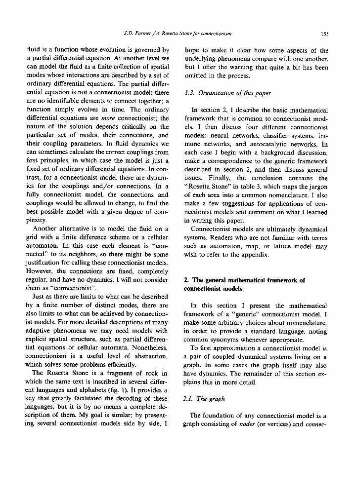
Fig. 1. "Ptolemy", in hieroglyphics, Demotic, and Greek. This cartouche played a seminal role in deciphering hieroglyphics, by providing a hint that the alphabet was partially phonetic [12]. (The small box is a "p" , and the half circle is a " t " - liter- ally it reads "ptolmis".)
1.1. Breaking the jargon barrier
Language is the medium of cultural evolution. To a large extent differences in language define culture groupings. Someone who speaks Romany, for example, is very likely a Gypsy; the existence of a common and unique language is one of the most important bonds preserving Gypsy culture. At times, however, communication between sub-
0167-2789/90/$03.50 © Elsevier Science Publishers B.V. (North-Holland)

154 J.D. Farmer/A Rosetta Stone for connec~omsm
cultures becomes essential, so that we must map one language to another.
The language of science is particularly special- ized. It is also particularly fluid; words are tools onto which we map ideas, and which we invent or redefine as necessary. Our jargon evolves as sci- ence changes. Although jargon is a necessary fea- ture of communication in science, it can also pose a barrier impeding scientific progress.
When models are based on a given class of phenomena, such as neurobiology or ecology, the terminology used in the models tends to reflect the phenomenon being modeled rather than the un- derlying mathematical structure. This easily ob- scures similarities in the mathematical structure. "Neura l activation" may appear quite different from "species population", even though relative to given mathematical models the two may be identi- cal. Differences in j argon place barriers to commu- nication that prevent results in one field from being transparent to workers in another field. Proper nomenclature should identify similar things but distinguish those that are genuinely different.
At present this problem is particularly acute for adaptive systems. The class of mathematical mod- els that are employed to understand adaptive systems contain subtle but nonetheless significant new features that are not easily categorized by conventional mathematical terminology. This adds to the problem of communication between disci- plines, since there are no standard mathematical terms to identify the features of the models.
1.2. What is connectionism?
Connectionism is a term that is currently ap- plied to neural network models such as those described in refs. [59, 15]. The models consist of elementary units, which can be "connected" together to form a network. The form of the resulting connection diagram is often called the architecture of the network. The computations performed by the network are highly dependent on the architecture. Each connection carries infor- mation in its weight, which specifies how strongly
the two variables it connects interact with each other. Since the modeler has control over how the connections are made, the architecture is plastic.
This contrasts with the lasual approach in dy- namics and bifurcation theory, where the dynami- cal system is a fixed object whose variability is concentrated into a few parameters. The plasticity of the connections and connection strengths means that we must think about the entire family of dynamical systems described by all possible archi- tectures and all possible combinations of weights. Dynamics occurs on as many as three levels, that of the states of the network, the values of connec- tion strengths, and the architecture of the connec- tions themselves.
Mathematical models with this basic structure are by no means unique to neural networks. They occur in several other areas, including classifier systems, immune networks, and autocatalytic net- works. They also have potential applications in other areas, such as economics, game-theoretic models and ecological models. I propose that the term connectionism be extended to this wider class of models.
By comparing connectionist models for different phenomena using a common nomenclature, we get a clear view of the extent to which these models are similar or different. We also get a glimpse of the extent to which the underlying phenomena are similar or different. I emphasize the word glimpse to make it clear that we are simplifying a compli- cated phenomenon when we model it in connec- tionist terms. Comparing two connectionist models of, for example, the nervous systems and the immune system, provides a means of extract- ing certain aspects of their similarities, but we must be very careful in doing this; much richness and complexity is lost at this level of description.
Connectionism represents a particular level of abstraction. By reducing the state of a neuron to a single number, we are collapsing its properties relative to a real neuron, or relative to those of another potentially more comprehensive mathe- matical formalism. For example, consider fluid dynamics. At one level of description the state of a
J.D. Farmer/A Rosetta Stone for connectionism 155
fluid is a function whose evolution is governed by a partial differential equation. At another level we can model the fluid as a finite collection of spatial modes whose interactions are described by a set of ordinary differential equations. The partial differ- ential equation is not a connectionist model; there are no identifiable elements to connect together; a function simply evolves in time. The ordinary differential equations are more connectionist; the nature of the solution depends critically on the particular set of modes, their connections, and their coupling parameters. In fluid dynamics we can sometimes calculate the correct couplings from first principles, in which case the model is just a fixed set of ordinary differential equations. In con- trast, for a connectionist model there are dynam- ics for the couplings a n d / o r connections. In a fully connectionist model, the connections and couplings would be allowed to change, to find the best possible model with a given degree of com- plexity.
Another alternative is to model the fluid on a grid with a finite difference scheme or a cellular automaton. In this case each element is "con- nected" to its neighbors, so there might be some justification for calling these connectionist models. However, the connections are fixed, completely regular, and have no dynamics. I will not consider them as "connectionist".
Just as there are limits to what can be described by a finite number of distinct modes, there are also limits to what can be achieved by connection- ist models. For more detailed descriptions of many adaptive phenomena we may need models with explicit spatial structure, such as partial differen- tial equations or cellular automata. Nonetheless, connectionism is a useful level of abstraction, which solves some problems efficiently.
The Rosetta Stone is a fragment of rock in which the same text is inscribed in several differ- ent languages and alphabets (fig. 1). It provides a key that greatly facilitated the decoding of these languages, but it is by no means a complete de- scription of them. My goal is similar; by present- ing several connectionist models side by side, I
hope to make it clear how some aspects of the underlying phenomena compare with one another, but I offer the warning that quite a bit has been omitted in the process.
1.3. Organization of this paper
In section 2, I describe the basic mathematical framework that is common to connectionist mod- els. I then discuss four different connectionist models: neural networks, classifier systems, im- mune networks, and autocatalytic networks. In each case I begin with a background discussion, make a correspondence to the generic framework described in section 2, and then discuss general issues. Finally, the conclusion contains the "Roset ta Stone" in table 3, which maps the jargon of each area into a common nomenclature. I also make a few suggestions for applications of con- nectionist models and comment on what I learned in writing this paper.
Connectionist models are ultimately dynamical systems. Readers who are not familiar with terms such as automaton, map, or lattice model may wish to refer to the appendix.
2. The general mathematical framework of connectionist models
In this section I present the mathematical framework of a "generic" connectionist model. I make some arbitrary choices about nomenclature, in order to provide a standard language, noting common synonyms whenever appropriate.
To first approximation a connectionist model is a pair of coupled dynamical systems living on a graph. In some cases the graph itself may also have dynamics. The remainder of this section ex- plains this in more detail.
2.1. The graph
The foundation of any connectionist model is a graph consisting of nodes (or vertices) and connec-

156 J.D. Farmer/A Rosetta Stone for connectionism
Cy c
a
d
Fig. 2. A directed graph.
tions (also called links or edges) between them as shown in fig. 2. The graph describes the architec- ture of the system and provides the channels in which the dynamics takes place. There are differ- ent types of graphs; for example, the links can be either directed (with arrows), or undirected (without arrows). For some purposes, such as modeling catalysis, it is necessary to allow compli- cated graphs with more than one type of node or more than one type of link.
For many purposes it is important to specify the pattern of connections, with a graph representa-
tion. The simplest way to represent a graph is to draw a picture of it, but for many purposes a more formal description is necessary. One common graph representation is a connection matrix. The nodes are assigned an arbitrary order, correspond- ing to the rows or columns of a matrix. The row corresponding to each node contains a nonzero entry, such as "1", in the columns corresponding to the nodes to which it makes connections. For example, if we order the nodes of fig. 2 lexico- graphically, the connection matrix is [ 101 ]
0 0 0 c = o 1 o . (1)
1 0 0 1 0 0
If the graph is undirected then the connection matrix is symmetric. It is sometimes economical to combine the representation of the graph and the connection parameters associated with it into a matrix of connection parameters.
A connection list is an alternative graph repre- sentation. For example, the graph of fig. 2 can also be represented as
a ~ b , a ~ d , b ~ a , c ~ c , d ~ b , e ~ b .
(2)
Note that the nodes are implicitly contained in the connection list. In some cases, if there are isolated nodes, it may be necessary to provide an addi- tional list of nodes that do not appear on the connection list. For the connectionist models dis- cussed here isolated nodes, if any, can be ignored.
A graph can also be represented by an algo- rithm. A simple example is a program that creates connections "a t random" using a deterministic random number generator. The program, together with the initial speed, forms a representation of a graph.
For a dense graph almost every node is con- nected to almost every other node. For a sparse graph most nodes are connected to only a small fraction of the other nodes. A connection matrix is a more efficient representation for a dense graph, but a connection list is a more efficient representa- tion for a sparse graph.
2.2. Dynamics
In conventional dynamical models the form of the dynamical system is fixed. The only part of the dynamical system that changes is the state, which contains all the information we need to know about the system to determine its future behavior. The possible ways the "fixed" dynamical form "might change" are encapsulated as parameters. These are usually thought of as fixed in any given experiment, but varying from experiment to exper- iment. Alternatively we can think of the parame- ters as knobs that can be slowly changed in the background. In reality the quantities that we in- corporate as parameters are usually aspects of the system that change on a time scale slower than those we are modeling with the dynamical system.

J.D. Farmer / A Rosetta Stone for connectionism 15 7
Connectionist models extend this view by giving the parameters an explicit dynamics of their own, and in some cases, by giving the list of variables and their connections a dynamics of its own. Typically this also involves a separation of time scales. Although a separation of time scales is not necessary, it provides a good starting point for the discussion. The fast scale dynamics, which changes the states of the system, is usually associated with short-term information processing. This is the transition rule. The intermediate scale dynamics changes the parameters, and is usually associated with learning. I will call this the parameter dynam- ics or the learning rule. On the longest time scale, the graph itself may change. I will call this the graph dynamics. The graph dynamics may also be used for learning; hopefully this will not lead to confusion.
Of course, strictly speaking the states, parame- ters, and graph representation described above are just the states of a larger dynamical system with multiple time scales. Reserving the word state for the shortest time scale is just a convenience. The association of time scales given above is the natu- ral generalization of "conventional" dynamical systems, in which the states change quickly, the parameters change slowly, and the graph is fixed. For some purposes, however, it might prove to be useful to relax this separation, for example, letting the graph change at a rate comparable to that of the states. Although all the models discussed here have at most three time scales, in principle this framework could be iterated to higher levels to incorporate an arbitrary number of time scales.
The information that resides on the graph typi- cally consists of integers, real numbers, or vectors, but could in principle be any mathematical ob- jects. The state transition and learning rules can potentially be any type of dynamical system. For systems with continuous states and continuous parameters the natural dynamics are ordinary differential equations or discrete time maps. In principle, the states or parameters could also be functions whose dynamics are partial differential equations or functional maps. This might be natu-
ral, for example, in a more realistic model of neurons where the spatio-temporal form of pulse propagation in the axon is important [60]. When the activities or parameters are integers, their dy- namics are naturally automata, although it is also common to use continuous dynamics even when the underlying states are discrete.
Since the representation of the graph is intrinsi- cally discrete, the graph dynamics usually has a different character. Often, as in classifier systems, immune networks, or autocatalytic networks, the graph dynamics contains random elements. In other cases, it may be a deterministic response to statistical properties of the node states or the connection strengths, for example, as in pruning algorithms. Dynamical systems with graph dynam- ics are sometimes called metadynamical systems [20, 8].
In all of the models discussed here the states of the system reside on the nodes of the graph .1. The states are denoted xi, where i is an integer label- ing the node. The parameters reside at either nodes or connections; 0i refers to a node parame- ter residing at node i, and w~j refers to a connec- tion parameter residing at the connection between node i and node j.
The degree to which the activity at one node influences the activity at another node, or the connection strength, is an important property of connectionist models. Although this is often con- trolled largely by the connection parameters w~j, the node parameters 0~ may also have an influ- ence, and in some cases, such as B-cell immune networks, provide the only means of changing the average connection strength. Thus, it is misleading to assume that the connection parameters are equivalent to the connection strengths. Since the connection strength of any given instant may vary depending on the states of the system, and since the form of the dynamics may differ considerably in different models, we need to discuss connection
**tit is also possible that states could be attached to connec- tions, bu t this is not the case in any of the models discussed here.

158 J.D. Farmer/A Rosetta Stone for connectionism
strength in terms of a quantity that is representa- tion-independent, which is well defined for any dynamical model.
For a continuous transition rule the natural way to discuss the connection strength is in terms of the Jacobian. When the transition rule is an ordi- nary differential equation, of the form
dx~ = f . (xx , x2, . . xN ) dt "' '
the instantaneous connection strength of the con- nection from node i to node j (where i is an input to j ) is the corresponding term in the Jacobian matrix
J / , = - a x , -
A connection is excitatory if J/i > 0 and inhibitory if J/~ < 0. Similarly, for discrete time dynamical systems (continuous maps), of the form
x j ( t + 1) = . f j ( x l , x 2 . . . . . x N ) ,
a connection is excitatory if Ij/il > 1 and in- hibitory if Ij/'il < 1. In a continuous system, the average connection strength is (J/i), where ( ) denotes an appropriate average; in a discrete sys- tem it is (IJ/A)- To make this more precise it is necessary to specify the ensemble over which the average is taken.
For automaton transition rules, since the states x~ are discrete the notion of instantaneous connec- tion strength no longer makes sense. The average connection strength may be defined in one of many ways; for example, as the fraction of times node j changes state when node i changes state. In situations where x~ is an integer but nonethe- less approximately preserves continuity, if I Ax~ (t) I is the magnitude of the change in x~ at time t, the average connection strength can be defined as
IAxj( t ÷ 1)
IAxi( t) I )lax,<Ol>0"
3. Neural nets
3.1. Background
Neural networks originated with early work of McCulloch and Pitts [42], Rosenblatt [58], and others. Although the form of neural networks was originally motivated by neurophysiology, their properties and behavior are not constrained by those of real neural systems, and indeed are often quite different. There are two basic applications for neural networks: one is to understand the properties of real neural systems, and the other is for machine learning. In either case, a central question for developing a theory of learning is: Which behaviors of real neurons are essential tc their information processing capabilities, and which are simply irrelevant side effects?
For machine learning problems neural networks have many uses that go considerably beyond the problem of modeling real neural systems. There are several reasons for dropping the constraints of modeling real neurons:
(i) We do not understand the behavior of real neurons.
(ii) Even if we understood them, it would be computationaUy inefficient to implement the full behavior of real neurons.
(iii) It is unlikely that we need the full complex- ity of real neurons in order to solve problems in machine learning.
(iv) By experimenting with different approaches to simplified models of neurons, we can hope to extract the basic principles under which they oper- ate, and discover which of their properties are truly essential for learning.
Because of the factors listed above, for machine learning problems there has been a movement towards simpler artificial neural networks that are less motivated by real neural networks. Such net- works are often called "artificial neural networks", to distinguish them from the real thing, or from more realistic models. Similar arguments apply to all the models discussed here; it might also be appropriate to say "artificial immune networks"
J.D. Farmer/A Rosetta Stone for connectionism 159
and "artificial autocatalytic networks". However, this is cumbersome and I will assume that the distinction between the natural and artificial worlds is taken for granted.
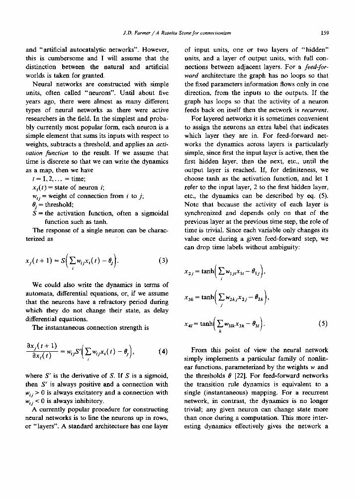
Neural networks are constructed with simple units, often called "neurons". Until about five years ago, there were almost as many different types of neural networks as there were active researchers in the field. In the simplest and proba- bly currently most popular form, each neuron is a simple element that sums its inputs with respect to weights, subtracts a threshold, and applies an acti- vation function to the result. If we assume that time is discrete so that we can write the dynamics as a map, then we have
t = I, 2 . . . . = time; x~(t) = state of neuron i; w~j = weight of connection from i to j ; Oj = threshold; S = the activation function, often a sigmoidal
function such as tanh. The response of a single neuron can be charac-
terized as
x,<,+1, -- -,,). (3)
We could also write the dynamics in terms of automata, differential equations, or, if we assume that the neurons have a refractory period during which they do not change their state, as delay differential equations.
The instantaneous connection strength is
of input units, one or two layers of "h idden" units, and a layer of output units, with full con- nections between adjacent layers. For a feed-for- ward architecture the graph has no loops so that the fixed parameters information flows only in one direction, from the inputs to the outputs. If the graph has loops so that the activity of a neuron feeds back on itself then the network is recurrent.
For layered networks it is sometimes convenient to assign the neurons an extra label that indicates which layer they are in. For feed-forward net- works the dynamics across layers is particularly simple, since first the input layer is active, then the first hidden layer, then the next, etc., until the output layer is reached. If, for definiteness, we choose tanh as the activation function, and let 1 refer to the input layer, 2 to the first hidden layer, etc., the dynamics can be described by eq. (5). Note that because the activity of each layer is synchronized and depends only on that of the previous layer at the previous time step, the role of time is trivial. Since each variable only changes its value once during a given feed-forward step, we can drop time labels without ambiguity:
(5)
Oxj( t + 1) = wijS' ( - 0 j ) , Oxi( t) ~i wijxi( t) (4)
where S' is the derivative of S. If S is a sigmoid, then S' is always positive and a connection with w~j > 0 is always excitatory and a connection with wij < 0 is always inhibitory.
A currently popular procedure for constructing neural networks is to line the neurons up in rows, or "layers". A standard architecture has one layer
From this point of view the neural network simply implements a particular family of nonlin- ear functions, parameterized by the weights w and the thresholds 0 [22]. For feed-forward networks the transition rule dynamics is equivalent to a single (instantaneous) mapping. For a recurrent network, in contrast, the dynamics is no longer trivial; any given neuron can change state more than once during a computation. This more inter- esting dynamics effectively gives the network a
160 J.D. Farmer/A Rosetta Stone for connectionism
memory, so that the set of functions that can be implemented with a given number of neurons is much larger. However, it becomes necessary to make a decision as to when the computation is completed, which complicates the learning prob- lem.
To solve a given problem we must select values of the parameters w and 0, i.e. we must select a particular member of the family of functions spec- ified by the network. This is done by a learning rule.
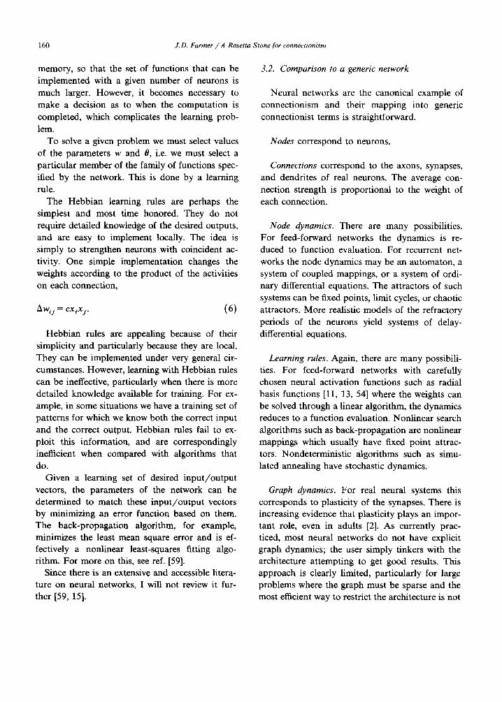
The Hebbian learning rules are perhaps the simplest and most time honored. They do not require detailed knowledge of the desired outputs, and are easy to implement locally. The idea is simply to strengthen neurons with coincident ac- tivity. One simple implementation changes the weights according to the product of the activities on each connection,
Aw, j = cxix j. (6)
Hebbian rules are appealing because of their simplicity and particularly because they are local. They can be implemented under very general cir- cumstances. However, learning with Hebbian rules can be ineffective, particularly when there is more detailed knowledge available for training. For ex- ample, in some situations we have a training set of patterns for which we know both the correct input and the correct output. Hebbian rules fail to ex- ploit this information, and are correspondingly inefficient when compared with algorithms that do.
Given a learning set of desired input /output vectors, the parameters of the network can be determined to match these input /output vectors by minimizing an error function based on them. The back-propagation algorithm, for example, minimizes the least mean square error and is ef- fectively a nonlinear least-squares fitting algo- rithm. For more on this, see ref. [59].
Since there is an extensive and accessible litera- ture on neural networks, I will not review it fur- ther [59, 15].
3.2. Comparison to a generic network
Neural networks are the canonical example of connectionism and their mapping into generic connectionist terms is straightforward.
Nodes correspond to neurons.
Connections correspond to the axons, synapses, and dendrites of real neurons. The average con- nection strength is proportional to the weight of each connection.
Node dynamics. There are many possibilities. For feed-forward networks the dynamics is re- duced to function evaluation. For recurrent net- works the node dynamics may be an automaton, a system of coupled mappings, or a system of ordi- nary differential equations. The attractors of such systems can be fixed points, limit cycles, or chaotic attractors. More realistic models of the refractory periods of the neurons yield systems of delay- differential equations.
Learning rules. Again, there are many possibili- ties. For feed-forward networks with carefully chosen neural activation functions such as radial basis functions [11, 13, 54] where the weights can be solved through a linear algorithm, the dynamics reduces to a function evaluation. Nonlinear search algorithms such as back-propagation are nonlinear mappings which usually have fixed point attrac- tors. Nondeterministic algorithms such as simu- lated annealing have stochastic dynamics.
Graph dynamics. For real neural systems this corresponds to plasticity of the synapses. There is increasing evidence that plasticity plays an impor- tant role, even in adults [2]. As currently prac- ticed, most neural networks do not have explicit graph dynamics; the user simply tinkers with the architecture attempting to get good results. This approach is clearly limited, particularly for large problems where the graph must be sparse and the most efficient way to restrict the architecture is not
J.D. Farmer/A Rosetta Stone for connectionism 161
obvious from the symmetries of the problem. There is currently a great deal of interest in implement- ing graph dynamics for neural networks, and there are already some results in this direction [26, 43, 46, 65, 67]. This is likely to become a major field of interest in the future.
4. Classifier systems
4.1. Background
The classifier system is an approach to machine learning introduced by Holland [30]. It was in- spired by many influences, including production systems in artificial intelligence [48], population genetics, and economics. The central motivation was to avoid the problem of brittleness encoun- tered in expert systems and conventional ap- proaches to artificial intelligence. The classifier system learns and adapts using a low-level ab- stract representation that it constructs itself, rather than a high-level explicit representation con- structed by a human being.
On the surface the classifier system appears quite different from a neural network, and at first glance it is not obvious that it is a connectionist system at all. On closer examination, however, classifier systems and neural networks are quite similar. In fact, by taking a sufficiently broad definition of "classifier systems" and "neural net- works", any particular implementation of either one may be viewed as a special case of the other. Classifier systems and neural networks are part of the same class of models, and represent two dif- ferent design philosophies for the connectionist approach to learning. The analogy between neural networks and classifier systems has been explored by Compiani et al. [14], Belew and Gherrity [9], and Davis [16]. There are many different versions of classifier systems; I will generally follow the version originally introduced by Holland [30], but with a few more recent modifications such as intensity and support [31].
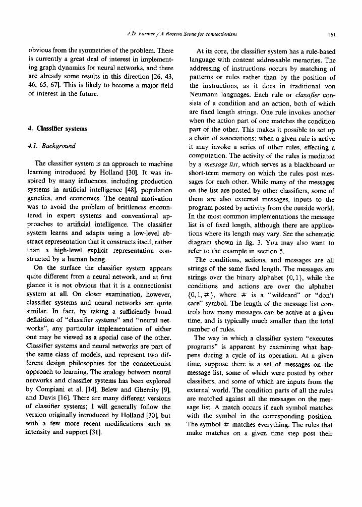
At its core, the classifier system has a rule-based language with content addressable memories. The addressing of instructions occurs by matching of patterns or rules rather than by the position of the instructions, as it does in traditional von Neumann languages. Each rule or classifier con- sists of a condition and an action, both of which are fixed length strings. One rule invokes another when the action part of one matches the condition part of the other. This makes it possible to set up a chain of associations; when a given rule is active it may invoke a series of other rules, effecting a computation. The activity of the rules is mediated by a message list, which serves as a blackboard or short-term memory on which the rules post mes- sages for each other. While many of the messages on the list are posted by other classifiers, some of them are also external messages, inputs to the program posted by activity from the outside world. In the most common implementations the message list is of fixed length, although there are applica- tions where its length may vary. See the schematic diagram shown in fig. 3. You may also want to refer to the example in section 5.
The conditions, actions, and messages are all strings of the same fixed length. The messages are strings over the binary alphabet (0,1}, while the conditions and actions are over the alphabet ( 0 , 1 , # } , where # is a "wildcard" or "don ' t care" symbol. The length of the message list con- trols how many messages can be active at a given time, and is typically much smaller than the total number of rules.
The way in which a classifier system "executes programs" is apparent by examining what hap- pens during a cycle of its operation. At a given time, suppose there is a set of messages on the message list, some of which were posted by other classifiers, and some of which are inputs from the external world. The condition parts of all the rules are matched against all the messages on the mes- sage list. A match occurs if each symbol matches with the symbol in the corresponding position. The symbol # matches everything. The rules that make matches on a given time step post their

162 J.D. Farmer/A Rosetta Stone for connectionism
Strength Condition Action Effector
-----7
v
Message list
!
External messages
Messages posted by classifiers
C lassifiers
Fig. 3. A schematic diagram of the classifier system.
actions as messages on the next time step. By going through a series of steps like this, the classi- fier system can perform a computation. Note that in most implementations of the classifier system each rule can have more than one condition part; a match occurs only when both conditions are
satisfied. In general, because of the # symbol, more than
one rule may match a given message. The parame- ters of the classifier system (frequency of # , length of messages, length of message list, etc.) are usu- ally chosen so that the number of matches typi- cally exceeds the size of the message list. The rules
then bid against each other to decide which of them will be allowed to post messages. The bids are used to compute a threshold, which is adjusted to keep the number of messages on the message list (that will be posted on the next step) less than or equal to the size of the message list. Only those rules whose bids exceed the threshold are allowed to post their messages on the next time step #2.
An important factor determining the size of the bid is the strength of a classifier, which is a real number attached to each classifier rule. The strength is a central part of the learning mecha- nism. If a classifier wins the bidding competit ion and successfully posts a message, an amount equal
~2Some implementations allow stochastic bidding.
to the size of its bid is subtracted from its strength and divided among the classifiers that (on the previous time step) posted the messages that match the bidding classifier's condition parts on the cur- rent time step #3.
Another factor in determining the size of bids is
the specificity of a classifier, which is defined as the percentage of characters in its condition part that are either zero or one, i.e. that are not # . The
motivation is that when there are "specialists" to solve a problem, their input is more valuable than that of "generalists".
The final factor that determines the bid size is the intensity xi(t ) associated with a given message. In older implementations of the classifier system, the intensity is a Boolean variable, whose value is one if the message is on the message list, and zero otherwise. In newer implementations the intensity is allowed to take on real values 0 < x i < 1. Thus, some messages on the list are "more intense" than others, which means they have more influence on subsequent activity. Under the support rule, the intensity of a message is computed by taking the sum over all the matching messages on the previ- ous time step, weighted by the strength of the classifier making the match.
*~3Other variants are also used. Many authors think that this step is unnecessary, or even harmful; this is a topic of active controversy.
J.D. Farmer/A Rosetta Stone for connectionism 163
The size of a bid is
bid = const × w × specificity × F(intensi ty) . (7)
F(intensity) is a function of the intensities of the matching messages. There are many options; for example, it can be the intensity of the message generating the highest bid, or the sum of the intensities of all the matching messages [57].
To produce outputs the classifier system must have a means of deciding when a computat ion halts. The most common method is to designate certain classifiers as outputs. When these classi- fiers become active the classifier system makes the
output associated with that classifier's message. If more than one output classifier becomes active it is necessary to resolve the conflict. There are vari-
ous means of doing this; a simple method is to simply pick the output with the largest bid.
Neglecting the learning process, the state of a classifier system is determined by the intensities of its messages (most of which may be zero). In many cases it is important to be able to pass along a particular set of information from one time step to another. This is done by a construction called pass-through. The # symbol in the action part of the rule has a different meaning than it has in the condition part of the rule. In the action part of the rule it is used to "pass through" information from the message list on one time step to the message list on the next time step; anywhere there is a # symbol in the action part, the message that is subsequently posted contains either a zero or a one according to whether the message matched by the condition part on the previous time step con- tained a zero or a one.
The procedure described above allows the clas- sifier system to implement any finite function, as long as the necessary rules are present in the
system with the proper strengths (so that the cor- rect rules will be evoked). The transfer of strengths according to bid size defines a learning algorithm called the bucket brigade. The problem of making sure the necessary rules are present is addressed by the use of genetic algorithms that operate on
the bit strings of the rules as though they were haploid chromosomes. For example, point muta- tions randomly changes a bit in one of the rules. Crossover or recombination mimics sexual repro-
duction. It is performed by selecting two rules, picking an arbitrary position, and interchanging substrings so that the left part of the first rule is concatenated to the right part of the second rule and vice versa. When the task to be performed has the appropriate structure, crossover can speed up the time required to generate a good set of rules, as compared to pure point mutat ion #4.
4.2. Comparison to generic network
The classifier system is rich with structure, nomenclature, and lore, and has a literature of its own that has evolved more or less independently of the neural network literature. Nonetheless, the two are quite similar, as can be seen by mapping the classifier system to standard connectionist terms.
For the purpose of this discussion we will as- sume that the classifiers only have one condition part. The extension to classifiers with multiple condition parts has been made by Compiani et al. [14].
Nodes. The messages are labels for the nodes of the connectionist network. For a classifier system with word length N the 2 N possible messages range from i = 0,1 . . . . . 2 N - 1. (In practice, for a
given set of classifiers, only a small subset of these
may actually occur.) The state of the i th node is the intensity x i. The node activity also depends on a globally defined threshold B(t), which varies in time.
Connections. The condition and action parts of the classifier rules are a connection list representa- tion of a graph, in the form of eq. (2). Each
*~4Several specialized graph manipulation operators, for ex- ample triggered cover operators, have also been developed for classifier systems [57].

1 6 4 J.D. Farmer/A Rosetta Stone for connectionism
classifier rule connects a set of nodes ( i } to a node j and can be written ( i} -*j . A rule consist-
ing entirely of ones and zeros corresponds to a single connection; a rule with n don' t care sym- bols represents 2" different connections. Note that if two rules share their output node j and some of their input nodes i then there are multiple connec-
tions between two nodes. The connection parame- ters w~j are computed as the product of the classi- fier rule strength and the classifier rule specificity,
i.e.
thus a more efficient graph representation, and pass-through is just a representational conve-
nience.
Transition rule. In traditional classifier systems a node j becomes active on time step t + 1 if it has an input connection i on time step t such that
x~(t)wij > 0. Using the support rule,
x j ( t + 1) = Y'~x i ( t ) wij, ( 8 ) i
Wij = specificity × strength.
When the graph is sparse there are many nodes that have no rule connecting them so that implic-
itly w~j = O. Note that only the connections are represented
explicitly; the nodes are implicitly represented by
the right-hand parts of the connection representa- tions, which give all the nodes that could ever conceivably become active. Thus nodes with no inputs are not represented. This can be very effi-
cient when the graph is sparse. Although on the surface pass-through appears
to be a means of keeping recurrent information, as first pointed out by Miller and Forrest [44], in connectionist terms it is a mechanism for efficient graph representation. Pass-through occurs when a classifier has # symbols at the same location in
both its condition and action parts. (If the # is only in the action part, then the pass-through value is always the same, and so it is irrelevant.)
The net effect is that the node that is activated on the output depends on the node that was active on the input. This amounts to representing more than one connection with a single classifier. For exam- ple, consider the classifier 0 # ~ 1 # . If node 00 becomes active, then the second 0 is "passed through", so the output is 10. Similarly, if 01 becomes active, the output is 11. The net result is that two connections are represented by the same classifier. F rom the point of view of the network, the classifier 0 # ~ 1 # is equivalent to the two classifiers 00 ~ 10 and 01 --, 11. The net effect is
where the sum is taken over all i that satisfy xi( t)wij > O. With the support rule the dynamics is thus piecewise linear, with nonlinearity due to the effect of the threshold 0. Without the support rule the intensity is x j ( t + 1) = maxi{x i ( t ) }.
There are two approaches to computing the
threshold 0. The simplest approach is to simply
set it to a constant value 0. A more commonly used approach in traditional classifier systems is to adjust O(t) on each time step so that the number of messages that are active on the message list is less than or equal to a constant, which is equivalent to requiring that the number of nodes active on a given time step is less than or equal to a constant. In connectionist terms this may be visualized as adding a special thresholding unit that has input and output connections to every node.
Learning rule. The traditional learning algo- r i thm for classifier systems is the bucket brigade, which is a particular modified Hebbian learning rule. (See eq. (6).) When a node becomes active,
strength is transferred from its active output connections to its active input connections. This transfer occurs on the time step after it was active. To be more precise,, consider a wave of activity x j ( t ) > 0 propagating through node j , as shown in
fig. 4. Suppose this activity is stimulated by m
activities xi( t - 1) > 0 through input connection parameters wij, and in turn stimulates activities x , ( t + 1) > 0 through output connection param- eters Wjk. Letting H be the Heaviside function

J.D. Farmer/A Rosetta Stone for connectionism 165
/ / / / / / / INPUTSOUTPUTS
i j k
Fig. 4. The bucket brigade learning algorithm. A wave of activ- ity propagates from nodes { i } at time t - 1 through node j at time t to nodes (k } at time t + 1. The solid lines represent active connections, and the dashed lines represent inactive connections. Strength is transferred from the input connections of j to output connections of j according to eq. (11). The motivation is that connections "pay" the connections that activate them.
H ( x ) = 1 for x > 0, H ( x ) = 0 for x < 0, the inpu t
connec t ions gain s t rength according to
xj Awij = -~ ~., wykH( xjwjk - 0) , (9)
k
Awjk = - xjwjI, H ( xjwjk - 0 ), (10)
where
Awij = wi j ( t + 1) - wij( t ) . (11)
Al l the quant i t i es on the r igh t -hand side are
eva lua ted at t ime t.
This is on ly one of several var iants of the bucke t
b r i ga de lea rn ing a lgor i thm; for d iscuss ion of o ther
poss ib i l i t ies see ref. [10].
In o rde r to learn, the system must receive
f eedback a b o u t the qual i ty of its pe r fo rmance .5.
To p rov ide f eedback abou t the overal l pe r fo rmance
#5It is clearly important to maintain an appropriate distri- bution of strength within a classifier system, which does not overly favor input or output classifiers and which can set up chains of appropriate associations. Strength is added to classi- tiers that participate in good outputs, and then the bucket brigade causes a local transfer of feedback, in the form of connection strength, from outputs to inputs. This is further complicated by the recursive structure of classifier systems, which corresponds to loops in the graph. Maintaining an appropriate gradient of strength from outputs to inputs has proved to be a difficult issue in classifier systems.
of the system, the ou tpu t connec t ions of the sys-
tem, or the effectors, are given s t rength accord ing
to the qua l i ty of their ou tputs . Judgemen t s as to
the qua l i ty mus t be m a d e accord ing to a predef ined
eva lua t ion funct ion. To p reven t the sys tem f rom
accumula t ing useless classifiers, causing i so la ted
connect ions , there is an ac t iv i ty tax which a moun t s
to a d i s s ipa t ion term. Put t ing all of these effects
together and fo l lowing ref. [21] we can wri te the
bucke t b r igade dynamics ( the lea rn ing rule) as
mwij~_ 1 m E xjwjkI4(xjw, k - o) k
- x iw i jH (xiwijO)
+ x i P ( t ) + kwij, (12)
where k is the d i s s ipa t ion ra te for the ac t iv i ty tax,
and P ( t ) is the eva lua t ion func t ion for ou tpu t s at
t ime t.
Graph dynamics. The g raph d y n a m i c s occurs
th rough m a n i p u l a t i o n s of the g raph r ep resen ta t ion
(the classifier rules) th rough genet ic a lgor i thms
such as po in t m u t a t i o n and crossover. These
ope ra t ions are s tochas t ic and are h ighly nonloca l ;
they preserve ei ther the inpu t or ou tpu t of each
connect ion , bu t the o ther pa r t can move to a very
different pa r t of the graph. The app l i ca t ion of
these ope ra to r s genera tes new connect ions , which
is usual ly a c c o m p a n i e d b y the remova l of o ther
connect ions .
4.3. An example
A n example makes the g raph- theore t i c view of
classifier sys tems clearer . F o r example , cons ider
the classic p r o b l e m of exclusive-or. (See also ref.
[9].) The exclusive-or func t ion is 0 if bo th inputs
are the same and 1 if bo th inpu t s are different.
The s t a n d a r d neura l net so lu t ion of this p r o b l e m
is easi ly i m p l e m e n t e d with three classifiers:
(i) 0 # -+ 10: + 1 ;
(ii) 0 # ---, 11: + 1 ;
(iii) 10 ---, 11: - 2 .

166 J.D. Farmer/A Rosetta Stone for connectionism
Table 1 A wave of activity caused by the inputs (1,1) is shown. The numbers from left to right are the intensifies on successive iterations. Initially the two input messages have intensity 1, and the others are 0. The input messages activate messages 10 and 11, and then 10 switches 11 off. For the input (0,0), in contrast, the network immediately settles to a fixed point with the intensities of all the nodes at zero.
node intensity
O0 1 1 1 1 O1 1 1 1 1 10 0 1 1 1 11 0 1 0 0
Fig. 5. A classifier network implementing the exclusive-or in standard neural net fashion. The binary numbers, which in classifier terms would be messages on the message fist, label the nodes of the network.
(The number after the colon is w = strength ×
specificity.) Although there are only three classi-
fiers, because of the # symbols they make five
connections, as shown in fig. 5.
With this representation the node 00 represents
one of the inputs, and 01 represents the other
input; the state of each input is its intensity. If
both inputs are 1, for example, then nodes 00 and
01 become active, in other words, they have inten-
sity > 0, which is equivalent to saying that the
messages 00 and 01 are placed on the message list.
Assume that we use the support rule, eq. (8), that
outputs occur when the activity on the message list settles to a fixed point, and that the message
list is large enough to accommodate at least four
messages. An example illustrating how the compu- tation is accomplished is shown in table 1.
This example is unusual from the point of view of common classifier system practice in several respects. (1) The protocol of requiring that the system settle to a fixed point in order to make an output. A more typical practice would be to make
an output whenever one of the output classifiers becomes active. (2) The message list is rather large
for the number of classifiers, so the threshold is never used. (3) There are no recursive connections (loops in the graph).
There are simpler ways to implement exclusive- or with a classifier system. For example, if we
change the input protocol and let the input mes-
sage be simply the two inputs, then the classifier
system can solve this with four classifiers whose
action parts are the four possible outputs. This
always solves the problem in one step with a
message list of length one. Note that in network
terms this corresponds to unary inputs, with the
four possible input nodes representing each possi-
ble input configuration. While this is a cumber-
some way to solve the problem with a network, it is actually quite natural with a classifier system.
4. 4. Comparison of classifiers and neural networks
There are many varieties of classifier systems
and neural networks. Once the classifier system is
described in connectionist terms, it becomes dif-
ficult to distinguish between them. In practice, however, there are significant distinctions between neural nets as they are commonly used and classi- fier systems as they are commonly used. The appro- priate distinction is not between classifiers and
neural networks, but rather between the two de-
sign philosophies represented by the typical imple- mentations of connectionist networks within the
classifier system and neural net communities. A comparison of classifier systems and neural net- works in a common language illustrates their

J.D. Farmer / A Rosetta Stone for connectionism 167
differences more clearly and suggests a natural synthesis of the two approaches.
Graph topology and representation. The connection list graph representation of the classifier system is efficient for sparse graphs, in contrast to the connection matrix representation usually favored by neural net researchers. This issue is not critical on small problems that can be solved by small networks which allow the luxury of a densely connected graph. On larger problems, use of a sparsely connected graph is essential. If a large problem cannot be solved with a sparsely connec- ted network, then it cannot feasibly be imple- mented in hardware or on parallel machines where there are inevitable constraints on the number of connections to a given node.
To use a sparse network it is necessary to discover a network topology suited to a given problem. Since the number of possible network topologies is exponentially large, this can be difficult. For a classifier system the sparseness of the network is controlled by the length of each message, and by the number of classifiers and their specificity. Genetic algorithms provide a means of discovering a good network, while maintaining the sparseness of the network throughout the learning process. (Of course, there may be problems with convergence time.) For neural nets, in contrast, the most commonly used approach is to begin with a network that is fully wired across adjacent layers, train the network, and then prune connections if their weights decay to zero. This is useless for a large problem because of the dense network that must be present at the beginning.
The connection list representation of the clas- sifier system, which can be identified with that of production systems, potentially makes it easier to incorporate prior knowledge. For example, Forrest has shown that the semantic networks of KL-One can be mapped into a classifier system [23]. On the other hand, another common form of prior knowledge occurs in problems such as vision, when there are group invariances such as translation
and rotation symmetry. In the context of neural nets, Giles et al. [25] have shown that such invari- ances can be hard-wired into the network by re- stricting the network weights and connectivity in the proper manner. This could also be done with a classifier system by imposing appropriate restrictions on the rules produced by the genetic algorithm.
Transition rule. Typical implementations of the classifier system apply a threshold to each input separately, before it is processed by the node, whereas in neural networks it is more common to combine the inputs and then apply thresholds and activation functions. It is not clear which of these approaches is ultimately more powerful, and more work is needed.
Most implementations of the classifier system are restricted to either linear threshold activation functions or maximum input activation functions. Neural nets, in contrast, utilize a much broader class of activation functions. The most common example is probably the sigmoid, but in recent work there has been a move to more flexible functions, such as radial basis functions [11, 13, 47, 54] and local linear functions [22, 35, 68]. Some of these functions also have the significant speed advantage of linear learning rules ~6. In smooth environments, smooth activation functions allow more compact representations. Even in en- vironments where a priori it is not obvious the smoothness plays a role, such as learning Boolean functions, smooth functions often yield better generalization results and accelerate the learning process [68]. Implementation of smoother activa- tion functions may improve performance of classifier systems in some problems.
Traditionally, classifier systems use a threshold computed on each time step in order to keep the number of active nodes below a maximum value. Computation of the threshold in this way requires
'~6Linear learning rules are sometimes criticized as "not local". Linear algorithms are, however, easily implemented in parallel by systolic arrays, and converge in logarithmic time.

168 J.D. Farmer/A Rosetta Stone for connectionism
a global computation that is expensive from a connectionist point of view. Future work should concentrate on constant or locally defined thresholds.
From a connectionist point of view, classifiers with the # symbol correspond to multiple connections constrained to have the same strength. There is no obvious reason why their lack of specificity should give them less connection strength. This intuition seems to be borne out in numerical experiments using simplified classifier systems [66].
Learning rule. The classifier system traditionally employs the bucket brigade learning algorithm, whose feedback is condensed into an overall performance score. In problems where there is more detailed feedback, for example a set of known input-output pairs, the bucket-brigade algorithm fails to use this information. This, combined with the lack of smoothness in the activation function, causes it to perform poorly in problems such as
Liqht chain f Poratope
° S EpiI°pe e p
| t o'o"ooo11'"o'ooo I Antibody Antibody Representation
~A' ntibody
Fig. 6. A schematic representation of the structure of an anti- body, an antibody as we represent it in our model, and a B-lymphocyte with antibodies on its surface that function as antigen detectors.
learning and forecasting smooth dynamical sys- tems [55]. Since there are now recurrent implementations of back-propogation [53], it makes sense to incorporate this into a classifier system with smooth activation functions, to see whether this gives better performance on such problems [9].
For problems where there is only a performance score, the bucket brigade is more appropriate. Unfortunately, there have been no detailed com- parisons of the bucket brigade algorithm against other algorithms that use "learning with a critic". The form of the bucket brigade algorithm is intimately related to the activation dynamics, in that the size of the connection strength transfers are proportional to the size of the input activation signal (the bid). Although coupling of the con- nection strength dynamics to the activation dynamics is certainly necessary for learning, it is not clear that the threshold activation level is the correct or only quantity to which the learning algorithm should be coupled. Further work is needed in this area.
5. Immune networks
5.1. Background
The basic task of the immune system is to distinguish between self and non-self, and to eliminate non-self. This is a problem of pattern learning and pattern recognition in the space of chemical patterns. This is a difficult task, and the immune system performs it with high fidelity, with an extraordinary capacity to make subtle distinc- tions between molecules that are quite similar.
The basic building blocks of the immune system are antibodies, " y " shaped molecules that serve as identification tags for foreign material; lympho- cytes, cells that produce antibodies and perform discrimination tasks; and macrophages, large cells that remove material tagged by antibodies. Lym- phocytes have antibodies attached to their surface which serve as antigen detectors. (See fig. 6.) For-

J.D. Farmer/A Rosetta Stone for connectionism 169
eign material is called antigen. A human contains roughly 10 20 antibodies and 1012 lymphocytes, organized into roughly 10 s distinct types, based on the chemical structure of the antibody. Each lym- phocyte has only one type of antibody attached to it. Its type is equivalent to the type of its attached antibodies. The majority of antibodies are free antibodies, i.e. not attached to lymphocytes. The members of a given type form a clone, i.e. they are chemically identical.
The difficulty of the problem solved by the immune system can be estimated from the fact that mammals have roughly 105 genes, coding for the order of 105 proteins. An antigenic determi- nant is a region on the antigen that is recognizable by an antibody. The number of antigenic determi- nants on a protein such as myoglobin is the order of 50, with 6 -8 amino acids per region. We can compare the difficulty of telling proteins apart to a more familar task by assuming that each antigenic determinant is roughly as difficult to recognize as a face. In this case the pattern recognition task performed by the immune system is comparable to recognizing a million different faces. A central question is the means by which this is accom- plished. Does the immune system function as a gigantic look up table, like a neural network with billions of "grandmother cells"? Or, does it have an associative memory with computational capa- bilities?
The argument given above neglects the impor- tant fact that there are 105 distinct proteins only if we neglect the immune system. Each antibody is itself a protein, and there are 10 s distinct anti- body, which appears to be a contradiction: How do we generate l0 s antibody types with only 105 genes? The answer lies in combinatorics. Each antibody is chosen from seven gene segments, and each gene segment is chosen from a "family" or set of possible variants. The total number of possi- ble antibody types is then the product of the sizes of each gene family. This is not known exactly, but is believed to be on the order of 107-108 . Additional diversity is created by somatic muta- tion. When the lymphocytes replicate, they do so
with an unusually large error rate in their anti- body genes. Although it is difficult to estimate the number of possible types precisely, it is probably much larger than the number of types that are actually present in a given organism.
The ability to recognize and distinguish self is learned. How the immune system accomplishes this task is unknown. However, it is clear that one of the main tools the immune system uses is clonal selection. The idea is quite simple: A particular lymphocyte can be stimulated by a particular anti- gen if it has a chemical reaction with it. Once stimulated it replicates, producing more lympho- cytes of the same type, and also secreting free antibodies. These antibodies bind to the antigen, acting as a " tag" instructing macrophages to re- move the antigen. Lymphocytes that do not recog- nize antigen do not replicate and are eventually removed from the system.
While clonal selection explains how the immune system recognizes and removes antigen, it does not explain how it distinguishes it from self. From both experiments and theoretical arguments, it is quite clear that this distinction is learned rather than hard-wired. Clonal selection must be sup- pressed for the molecules of self. How this actu- ally happens is unknown.
A central question for self-nonself discrimina- tion is: Where is the seat of computation? It is clear that a significant amount of computation takes place in the lymphocytes, which have a sophisticated repertoire of different behaviors. It is also clear that there are complex interactions be- tween lymphocytes of the same type, for example, between the different varieties of T-lymphocytes and B-lymphocytes. These interactions are partic- ularly strong during the early stages of develop- ment.
Jerne proposed that a significant component of the computational power of the immune system may come from the interactions of different types of antibodies and lymphocytes with each other [33, 34]. The argument for this is quite simple: Since antibodies are after all just molecules, then from the point of view of a given molecule other
170 J.D. Farmer / A Rosetta Stone for connectionism
molecules are effectively indistinguishable from antigens. He proposed that much of the power of the immune system to regulate its own behavior may come from interacting antibodies and lym- phocytes of many different types .7.
There is good experimental evidence that net- work interactions take place, particularly in young animals. Using the nomenclature that an antibody that reacts directly with antigen AB1, an antibody that reacts directly with AB1 is AB2, etc., antibod- ies in categories as deep as AB4 have been ob- served experimentally #8. Furthermore, rats raised in sterile environments have active immune sys- tems, with activity between types. Nonetheless, the relevance of networks in immunology is highly controversial.
5.2. Connectionist models of the immune system
While Jerne proposed that the immune system could form a network similar to that of the ner- vous system, his proposal was not specific. Early work on immune networks put this proposal into more quantitative terms, assuming that a given AB1 type interacted only with one antigen and one other AB2 type. These interactions were mod- eled in terms of simple differential equations whose three variables represented antigen, AB1, and AB2 [56, 28]. A model that treats immune interactions in a connectionist network #9, allowing interac- tions between arbitrary types, was proposed in ref. [21]. The complicated network of chemical inter- actions between different antibody types, which are impossible to model in detail from first princi- ples, was taken into account by constructing an artificial antibody chemistry. Each antigen and antibody type is assigned a random binary string, describing its "chemical properties". Chemical in- teractions are assigned based on complementary
~TSuch networks are often called idiotypic networks. *~SThis classification of antibodies should not be confused
with their type; a given type can simultaneously be AB1 and AB2 relative to different antigens, and many different types may be AB1.
#gAnother connectionist model with a somewhat different philosophy was also proposed by Hoffmann et al. [29].
matching between strings. The strength of a chem- ical reaction is proportional to the length of the matching substrings, with a threshold below which no reaction occurs. Even though this artificial chemistry is unrealistic in detail, hopefully it cor- rectly captures some essential qualitative features of real chemistry.
A model of gene shuffling provides metady- namics for the network. This is most realistically accomplished with a gene library of patterns, mimicking the gene families of real organisms. These families are randomly shuffled to produce an initial population of antibody types. This gives an initial assignment of chemical reactions, through the matching procedure described above, including rate constants and other parameters #1°. Kinetic equations implement clonal selection; some types are stimulated by their chemical reac- tions, while others are suppressed. Types with no reactions are slowly flushed from the system so that they perish. Through reshuffling of the gene library new types are introduced to the system. It is also possible to stimulate somatic mutation through point mutations of existing types, propor- tional to their rate of replication.
It is difficult to model the kinetics of the im- mune system realistically. There are five different classes of antibodies, with distinct interactions and properties. There are different types of lym- phocytes, including helper, killer and supressor T-cells, which perform regulatory functions, as well as B-cells, which can produce free antibodies. All of these have developmental stages, with dif- ferent responses in each stage. Chemical reactions include cell-cell, antibody-antibody, and cell-an- tibody interactions. Furthermore, the responses of cells are complicated and often state dependent. Thus, any kinetic equations are necessarily highly approximate, and applicable to only a subset of the phenomena.
In our original model we omitted T-cells, treat- ing only B-cells. (This can also be thought of as
~*l°The genetic operations described here are more sophisti- cated than those actually used in ref. [21]; more realistic mechanisms have been employed in subsequent work [50, 17, 18].

J.D. Farmer/,4 Rosetta Stone for connectionism 171
modeling the response to certain polymeric anti- gens, for which T-cells seem to be irrelevant.) We assumed that the concentration of free antibodies is in equilibrium with the concentration of lym- phocytes, so that their populations can be lumped together into a single concentration variable. Since the characteristic time scale for the production of free antibodies is minutes or hours, while that of the population of lymphocytes is days, this is a good approximation for some purposes. It turns out, however, that separating the concentration of lymphocytes and free antibodies and considering the cell-cell, antibody-antibody, and cell-anti- body reactions separately give rise to new phe- nomena that are important for the connectionist view. In particular, this generates a more interest- ing repertoire of steady states, including "mildly excited" self-stimulated states suggestive of those observed in real immune systems [50, 17, 18].
5.3. Comparison to a generic network
As with classifier systems and neural networks, there are several varieties of immune networks [21, 17, 29, 64], and it is necessary to choose one in order to make a comparison. The model described here is based on that of Farmer, Packard and Perelson [21], with some modifications due to later work by Perelson [50] and De Boer and Hogeweg [17]. Also, since this model only describes B-cells, whenever necessary I will refer to it as a B-cell network, to distinguish it from models that also incorporate the activity of T-cells.
To discuss immune networks in connectionist terms it is first necessary to make the appropriate map to nodes and connections. The most obvious mapping is to assign antibodies and antigens to nodes. However, since antibodies and antigens typically have more than one antigenic determi- nant, and each region has a distinct chemical shape .11, we could also make the regions (or
*11"Chemical shape" here means all the factors that influ- ence chemical properties, including geometry, charge, polariza- tion, etc.
chemical shapes) the fundamental variable. Since all the models discussed above treat the concentra- tion of antibodies and lymphocytes as the funda- mental variables, I shall make the identification at this ]level. This leads to the following connectionist description:
~odes correspond to antibodies, or more accur- ately, to distinct antibody types. Antigens are anolher type of node with different dynamics; from a certain point of view the antigen concen- trations may be regarded as the input and output nodes of the network #12. The free antibody con- centrations, which can change on a rapid time scale, are the states of the nodes. They are the immediate indicators of information processing in the network. The lymphocyte concentrations, which change on an intermediate time scale, are node parameters. (Recall that there is a one-to-one correspondence between free antibody types and lymphocyte types.) Changes in lymphocyte concentration are the mechanism for learning in the network.
Connections. The physical mechanisms which cause connections between nodes are chemical reactions between antibodies, lymphocytes, and antigens. The strength of the connections depends on the strength of the chemical reactions. This is in part determined by chemical properties, which are fixed in time, and in part by the concentrations of the antibodies, lymphocytes, and antigens, which change with time. Thus the instantaneous connection strength changes in time as conditions change in the network. The precise way of representing and modeling the connections is explained in more detail in the following.
Graph representation. To model the notion of "chemical properties" we assign each antibody type a binary string. To determine the rate of the chemical reaction between type i and type j, the binary string corresponding to type i is compared
#12Future models should include chemical types identified with self as yet another type of node.

172 J.D. Farmer/A Rosetta Stone for connectionism
to binary string corresponding to type j. A match strength matrix mij is assigned to this connection, which depends on the degrees of complementary matching between the two strings. Types whose strings have a high degree of complementary matching are assigned large reaction rates. Since the matching algorithm is symmetric #13 mij = mji.
There is a threshold for the length of the complementary matching region below which we assume that no reaction occurs and set mij = O.
Since mq is the connection matrix of the graph, s e t t i n g m i j = 0 amounts to deleting the corres- ponding connection from the graph. We thus neglect reactions that are so weak that they have an insignificant effect on the behavior of the network. The match threshold together with the length of the binary strings determines the sparseness of the graph. When the system is sparse the matrix mij can be represented in the form of a connection list. The match strength for a given pair of immune types does not change with time. However, as new types are added or deleted from the system, the mij that are relevant to the types in the network change.
The graph dynamics provides a mechanism of learning in the immune system; as new types are tested by clonal selection, the graph changes, and the system "evolves". Another mechanism for dynamical learning depends on the lymphocyte concentrations, as discussed below.
Dynamics. The mq are naturally identified as connection parameters for the network. For any given i and j, however, the m~j are fixed. Thus, in B-cell immune networks the parameter dynamics, analogous to the learning rule in neural networks, occurs not by changing connection parameters, but rather by changing the lymphocyte concen- tration, which is a parameter node. The net reaction flux (or strength of the reaction) is a nonlinear function of the lymphocyte concen-
**13In our original paper [21] we also considered the case of asymmetric interactions. However, this is difficult to justify chemically, and it is probably safe to assume that the connec- tions are symmetric [28].
trations. Thus changing the lymphocyte concen- tration changes the effective connection strength. This is a fundamental difference between neural networks and B-cell immune networks; while the connection strength is changeable in both cases, in B-cell immune networks all the connection strengths to a given node change in tandem as the lymphocyte concentration varies. However, since the reaction rates are nonlinear functions, a change in lymphocyte concentration may affect each con- nection differently, depending on the concentration of the other nodes.
The dynamics of the real immune system are not well understood. The situation is similar to that of neural networks; we construct simplified heuristic immune dynamics based on a combina- tion of chemical kinetics and experimental observations, attempting to recover some of the phenomena of real immune systems. The real complication arises because lymphocytes are cells, and understanding their kinetics requires under- standing how they respond to stimulation and suppression by antigens, antibodies, and other cells. At this point our understanding of this is highly approximate and comes only from experimental data. The kinetic equations used in our original paper were highly idealized [21]. The more realistic equations quoted here are due to De Boer and Hogeweg #14 [17].
Let i label the nodes of the system, x i the concentration of antibodies, and #i the concen- tration of lymphocytes #15. The amount of stimulation received by lymphocytes of type i is approximated as
s, = Y'~mijx j. (13) J
The rate of change of antibody concentration is
#14More realistic equations have also been proposed by Segel and Perelson [61], Perelson [51, 50], and Varela et al. [64].
#15Note that I use 8 to represent lymphocytes because they play the role of node parameters. However, they are not thresholds, but rather quantities whose primary function is to modify connection strength.
J.D. Farmer/A Rosetta Stone for connectionism 173
due to production by lymphocytes, removal from the system, and binding with other antibodies. The equations are
d x i a t = o f f ( s , ) - kx~ - cx ,s , . (14)
k is a dissipation constant and c the binding constant, f is a function describing the degree of stimulation of a lymphocyte. Experimental obser- vations show that f is bell-shaped. A function with this rough qualitative behavior can be constructed by taking the product of a sigmoid with an inverted sigmoid, for example
z k 2 f ( z ) = (k x + z ) ( k 2 + z ) . (15)
The product ion of lymphocytes is due to replenishment by the bone marrow, cell replica- tion, and removal from the system. The equations a r e
dO, - r + p O J ( s , ) - kO~. (16)
d t
r is the rate of replenishment and p is a rate constant for replication.
5.4. Compar i son to neural ne tworks and classifier
s y s t ems
There are significant differences between the dynamics of immune networks and neural net- works. The most obvious is in the form of the transition and learning rules. The nodes of the immune network are activated by a bell-shaped function rather than a sigmoid function. Since the bell-shaped function undergoes an inflection and its derivative changes sign, the dynamics are po- tentially more complicated.
B-cell immune networks differ from neural net- works in that there is no variable which acts as a
connection parameter. Instead, the connection strength is indirectly determined by the node pa- rameters (concentrations and kinetic equations). The instantaneous connection strength is
3x j - [ Oi f ' ( s i ) - cxi] miJ - csi - k 3 i j ' (17)
where 3ij = 0 for i 4:j, 8, = 1. All of the terms in this equation except for f ' are greater than or equal to zero. For low values of s i, f ' ( s , ) > 0, but for large values of s i, f ' ( s i ) < 0. Given the struc- ture of these equations, as s~ increases, at some point before f reaches a maximum, all the connec- tions to a given node change from excitatory to inhibitory. The point at which this happens de- pends on the lymphocyte concentration of i, the antibody concentration, the concentration of the other antibodies, and on the exact form of the stimulation function. Thus, in contrast to neural networks or the classifier system, a given connec- tion can be either excitatory or inhibitory depend- ing on the state of the system.
The connections in the immune system are chemical reactions. Insofar as the immune system is well stirred, this allows a potentially very large connectivity, as high as the number of different chemical types a given type can react with. In practice, t h e number of types that a given type reacts with can be as high as about 1000. Thus, the connectivity of real immune networks is appar- ently of the same order of magnitude as that of real neural networks.
One of the central differences between the B-cell immune networks and neural or classifier net- works is that for the immune system there are no independent parameters on the connections. If the average strength of a connection to a given node cannot be adjusted independently of that of other nodes, the learning capabilities of the network may be much weaker or more inefficient than those of networks where the connection parame- ters are independent. As discussed in section 5.5, this may be altered by the inclusion of T-cells in the models.

174 J.D. Farmer/A Rosetta Stone for connectionism
5. 5. Directions for future research
Whether immune networks are a major compo- nent of the computational machinery of the im- mune system is a subject of great debate. The
analogy between neural networks and immune networks suggests that immune networks poten- tially possess powerful capabilities, such as asso- ciative memory, that could be central to the functioning of the immune system. However, be- fore this idea can reach fruition we need more demonstrat ions of what immune networks can do. At this point the theory of immune networks is still in its infancy and their utility remains an
open question. The immune network may be able to perform
tasks that would be impossible for individual cells.
Cons ider , for example, a large antigen such as a bacterium with many distinct antigenic determi-
nants. If each region is chemically distinct, a sin- gle type can interact with at most a few of them (and thus a single cell can interact with at most a few of them). Network interactions, in contrast, potentially allow different cells and cell types to communicate with each other and make a collec- tive computat ion to reinforce or suppress each o the r ' s immune responses. For example, suppose A, B, C and D are active sites. It might be useful for a network to implement an associative mem- ory rule such as: If any three of A, B, C, and D are present, then generate an immune response;
otherwise do not. Such an associative memory requires the capability to implement a repertoire
of Boolean functions. A useful rule might be: "Genera te an immune response if active site A is present, or active site B ispresent, but not if both are present simultaneously". Such a rule, which is equivalent to taking the exclusive-or function of A and B, might be useful for implementing self tolerance. Such logical rules are easily imple- mented by networks. It is difficult to see how they could be implemented by individual cells acting
on their own. Immune memory is another task in which net-
works may play an essential role. Currently the
prevailing belief is that immune memory comes about because of special memory cells. It is cer- tainly true that some cells go into developmental
states that are indicative of memory. Although the typical lifetime of a lymphocyte is about five days, there are some lymphocytes that have been
demonstrated to persist for as long as a month. This is a far cry, however, from the eighty or more years that a human may display an immune mem- ory. Since cells are normally flushed from the system at a steady rate, it is difficult to believe that any individual cell could last this long. It is only the type, then, that persists, but in order to achieve this individual cells must periodically replicate themselves. However, in order to hold the popula- tion stable the replication rate must be perfectly balanced against the removal rate. This is an un-
stable process unless there is feedback holding the population stable. It is difficult to see how feed- back on the population size can be given unless
there are network interactions. In an immune network a memory can poten-
tially be modeled by a fixed point of the network. The concentrations at the fixed point are held constant through the feedback of one type to another type. Models of the form of eqs. (14) and (16) contain fixed points that might be appropri- ate for immune memory. However, it is clear from experiments that T-cells are necessary for mem- ory, and so must be added to immune networks to
recover this effect. T-cells are a key element missing from most
current immune network models. T-cells play an important role in stimulating or suppressing reac- tions between antibodies and antigens, and are essential to immune memory. From the point of view of learning in the network, they may also indirectly act as specific connection parameters.
One of the most interesting activities of the immune system is "ant igen presentation". When a B-cell or macrophage reacts with an antigen it may process it, discarding all but the antigenic determinants. It then presents the antigenic deter- minant on its surface (as a peptide bound to an M H C molecule). The T-cell reacts with the anti-
J.D. Farmer/A Rosetta Stone for connectionism 175
genic determinant and the B-cell, and based on this information may either stimulate or suppress the B-cell. Note that antigen presentation provides information about both the B-cell and an antigen, and thus potentially about a specific connection in the network.
In a connectionist model, this may amount to a connection strength parameter; a B-cell presenting a given active site contains information that is specific to two nodes, one for the B-cell of the same type as the T-cell, and one for the antigen whose active site is being presented (which may also be another antibody). Due to their interac- tions with T-cells, the B-cell populations of type i presenting antigenic determinants from type j may play the roles of the connection parameters wij.
At this point, it is not clear how strongly the absence of explicit connection parameters limits the computational and learning power of immune networks. However, it seems likely that before they can realize their full potential, connection parameters must be included, taking into account the operation of T-cells. T-cells act like catalysts, either suppressing or enhancing reactions. Since catalytic activity is one of the primary tools used to implement the internal functions of living or- ganisms, it is not surprising that it should play a central role in the immune system as well. Auto- catalytic activity is discussed in more detail in section 6.
6. Autocatalytic networks
6.1. Background
All the models discussed so far are designed to perform learning tasks. The autocatalytic network model of this section differs in that it is designed to solve a problem in evolutionary chemistry. Of course, evolution may also be regarded as a form of learning. Still, the form that learning takes in autocatalytic networks is significantly different from the other models discussed here.
The central goal of the autocatalytic network is to solve a classic problem in the origin of life,
namely, to demonstrate an evolutionary pathway from a soup of monomers to a polymer metabolism with selected autocatalytic properties, which in turn could provide a substrate for the emergence of contemporary (or other) life forms. When Miller and Urey discovered that amino acids could be synthesized de novo from the hypothetical primor- dial constituents "earth, fire and water" [45], it seemed but a small step to the synthesis of poly- mers built out of amino acids (polypeptides and proteins). It was hoped that RNA and DNA could be created similarly. However, under normal cir- cumstances longer polymers are not favored at equilibrium. Living systems, in contrast, contain DNA, RNA, and proteins, specific long polymers which exist in high concentration. They are main- tained in abundance by their symbiotic relation- ship with each other: Proteins help replicate RNA and DNA, and DNA and RNA help synthesize proteins. Without the other, neither would exist. How did such a complex system ever get started, unless there were proteins and RNA to begin with? The question addressed in refs. [36, 20, 8] is: Under what circumstances can the synthesis of specific long polymers be achieved beginning with simple constituents such as monomers and dimers?
The model here applies to any situation in which unbranched polymers are built out of monomers through a network of catalytic activity. The monomers come from a fixed alphabet, a, b, c , . . . They form one-dimensional chains which are rep- resented as a string of monomers, acabbacbc.. . The monomer alphabet could be the twenty amino acids, or it could equally well be the four nu- cleotides. This changes the parameters but not the basic properties of the model. The model assumes that the polymers have catalytic properties, i.e. that they can undergo reactions in which one polymer catalyzes the formation of another. If A, B, C, and E are polymers, and H is water, then the basic reaction is:
E A + B # C + H , (18)
where E is written over the arrows to indicate that it catalyzes the reaction.

176 J.D. F a r m e r / A Rosetta Stone fo r connectionism
Our purpose is to model a chemostat, a reaction vessel into which monomers are added at a steady rate. The chemical species that are added to the chemostat are called the food set. We assume that the mass in the vessel is conserved, for example, by simply letting the excess soup overflow. For convenience we assume that the soup is well stirred, so that we can model it by a system of ordinary differential equations.
In any real system it is extremely difficult to determine from first principles which reactions will be catalyzed, and with what affinity. Very few if any of the relevant properties have been mea- sured experimentally in any detail, and the num- ber of measurements or computations that would have to be made in order to predict all the chemi- cal properties is hopelessly complex. Our ap- proach is to invent an artificial chemistry and attempt to make its properties at least qualita- tively similar to those of a real chemical system. Actually we use one of two different artificial chemistries, based on two different principles:
(i) Random assignment of catalytic properties. (ii) Assignment of catalytic properties based on
string matching. These two simple artificial chemistries lie on the
borders of extreme behavior in real chemistry. In some cases, we know that changing one monomer can have a dramatic effect on the chemical proper- ties of a polymer, either because it causes a drastic change in the configuration of the polymer or because it alters a critical site. If this were always the case, then random chemistry would be a rea- sonable model.
In other cases, changing a monomer has only a small effect on the chemical properties. Our string matching model is closer to this case; altering a single monomer will only change the quality of matching between two strings by an incremental amount, and should never cause a dramatic alter- ation in the chemical properties of the polymer.
Another difficulty of modeling real chemistry is that there is an extraordinarily large number of possible reactions. In a vessel with all polymers of length l or less, for example, the total number
of polymer species is x~i=t" t where m is the ~..,i--1 eft ,
number of distinct monomers. For example, with m = 20 and l = 100, the number of polymer species is in excess of 201°° , an extremely large number, and the number of possible reactions is still larger than this. To get around this problem, to first approximation, we neglect spontaneous reactions, and assume that the catalytic properties are suf- ficiently strong that all catalyzed reactions are much faster than spontaneous reactions #16.
Once we have assigned chemical properties, we can represent the network of catalyzed chemical reactions as a graph, or more precisely, as a poly- graph with two types of nodes and two types of connections [20]. Because of catalysis the graph must be more complicated than for any of the other networks discussed so far. An example is shown in fig. 7. One type of node is labeled by ovals containing the string representation of the polymer species. The other type of node corre- sponds to catalyzed reactions, and is labeled by black dots. The dark black connections are undi- rected (because the reactions are reversible), and connect each reaction to the three polymer species that participate in it; the dotted connections are directed, and connect the reaction to its catalysts. All the edges connect polymers to reactions, and each reaction has at least four connections, three connections for the reaction products and one or more for the catalyst(s). In this illustration we have labeled the members of the food set by double ovals.
If we use the random method of assigning chemical properties, then the graph is a random graph and can be studied using standard tech- niques. The probability p that a reaction selected at random will be catalyzed controls the ratio of connections to nodes. As p increases so does this
#16In more recent work [7] we make a tractable model for approximate treatment of spontaneous reactions by lumping together all the polymer species of a given length that are not in the autocatalytic network, assuming that they all have the same concentration. These can be viewed as a new type of node in the network. This allows us to include the effect of spontaneous reactions when necessary.
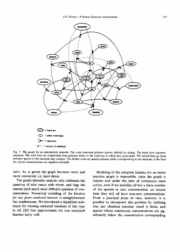
J.D. Farmer / A Rosetta Stone for connectionism 177
u b u b b b
0 ~ 0 J 0 Q 0
o °
l=klmabbbab
6 U D O 9 O O I Q 0 O O 4
= f o o d set
0 = other chemicals
= reactions
• . . . . . = a c t i o n o f c a t a l y s t s
Fig. 7. The graph for an autocatalytic network. The ovals represent polymer species, labeled by strings. The black dots represent reactions. The solid lines are connections from polymer nodes to the reactions in which they participate. The dotted lines go from polymer species to the reactions they catalyze. The double ovals are special polymer nodes corresponding to the elements of the food set, whose concentrations are supplied externally.
ratio. As p grows the graph becomes more and more connected, i.e. more dense.
The graph-theoretic analysis only addresses the question of who reacts with whom, and begs the central (and much more difficult) question of con- centrations. Numerical modeling of the kinetics for any given catalyzed reaction is straightforward but cumbersome. We introduced a simplified tech- nique for treating catalyzed reactions of this type in ref. [20] that approximates the true catalyzed kinetics fairly well.
Modeling of the complete kinetics for an entire reaction graph is impossible, since the graph is infinite and under the laws of continuous mass action, even if we initialize all but a finite number of the species to zero concentration, an instant later they will all have non-zero concentrations. From a practical point of view, however, it is possible to circumvent this problem by realizing that any chemical reaction vessel is finite, and species whose continuous concentrations are sig- nificantly below the concentration corresponding

178 J.D. Farmer / A Rosetta Stone for connectionism
to the presence of a single molecule are unlikely to participate in any reactions. Thus, to cope with this problem we introduce a concentration thresh- old, and only consider reactions where all the members on either side of the reaction equation (either A, B, and E, or C and E) are above the concentration threshold. This then becomes a metadynamical system: At any given time, only a finite number of species are above the threshold, and we only consider a finite graph. As the kinet- ics act, species may rise above the concentration threshold, so that the graph grows, or they may drop below the threshold, so that the graph shrinks.
One of the main goals of this model is to obtain closure in the form of an autocatalytic set, which is a set of polymer species such that each member of the set is produced by at least one catalyzed reaction involving only other members of the set (including the catalysts). Since the reactions are reversible, a species can be "produced" either by cleavage or condensation, depending on which side of equilibrium it finds itself. Thus an autocat- alytic set can be quite simple; for example,
A A + B ~ C + H (19)
is an autocatalytic set, and so is
A + B C c + H . (20)
A, B, and C will be regenerated by supplying either A and B, or by supplying C. Note, however, that such simple autocatalytic sets are only likely to occur when the probability of catalysis is very high. Even for small values of p it is always possible to find autocatalytic sets as long as the food set is big enough. However, the typical auto- catalytic set is more complicated than the exam- pies given in eqs. (19) and (20). There is a critical transition from the case where graphs with auto- catalytic sets are very rare to that in which they are very common, as described in refs. [20, 36]. The results given there show that it is possible to create autocatalytic sets (in this graph theoretic
sense) under reasonably plausible prebiotic condi- tions.
There are three notions of the formation of autocatalytic sets, depending on what we mean by "produced by" in the definition given above:
(i) Graph theoretic. The subgraph defined by the autocatalytic set is closed, so that each member is connected (by a solid connection) to at least one reaction catalyzed by another member.
(ii) Kinetics. Each member is produced at a level exceeding a given concentration threshold.
(iii) Robust. The autocatalytic set is robust un- der at least some changes in its food set, i.e. its members are at concentrations sufficiently large and there are enough pathways so that for some alterations of the food set it remains a kinetic autocatalytic set, capable of regenerating removed elements at concentrations above the threshold.
These notions are arranged in order of their strength, i.e. an autocatalytic set in the sense of kinetics is automatically an autocatalytic set in the graph-theoretic sense, and a robust autocatalytic set is automatically a kinetic autocatalytic set.
Describing the details of the conditions under which autocatalytic sets can be created is outside of the scope of this paper. Suffice it to say that, within our artificial chemistry we can create ro- bust autocatalytic sets. Consider, for example, an autocatalytic set based on the monomers a and b, originally formed by a food set consisting of the species a, b, ab, and bb, as shown in fig. 8 and table 2.
We plot the concentrations of the 21 polymer species in the reactor against an index that is arbitrary except that it orders the species accord- ing to their length. We compare four different alterations of the original food set, all of which have the same rate of mass input. For two of the altered food sets the concentration of the members of the autocatalytic set remains almost the same; they are all maintained at high concentration. For the other two, the autocatalytic set "dies" in that some of the members of the set fall below the concentration threshold, and most of the concen- trations decrease dramatically [7].

J.D. Farmer / .4 Rosetta Stone for connectionism 179
0
0 r.)
lO
1
o.1
O.Ol
o.ooi
o.oooi
1o-6
lO -6
1o-7
10 -a 0
/•'A' ' I ' ' ' ' I '
f V
l"
! " .-x • ~-
F
I"
I0 20
Poly
Fig. 8. An experiment demonstrating the robust properties of an autocatalytic set. The food set is originally a, b, ab, and bb. The food set is altered in four different ways, as shown in table 2. For each alteration of the food set the concentrations of all 21 polymers in the autocatalytic set are plotted against the "polymer index". (The polymer index assigns a unique label to each polymer. It is ordered according to length, but is other- wise arbitrary.) Two of the alterations of the food set cause the autocatalytic set to die, while the other two hardly change it. Like a robust metabolism, the autocatalytic set can digest a variety of different foods.
Table 2 An experiment in varying the food set of an autocatalytic set. The table shows the four species of the food set, and the concentration of each that is supplied externally per unit time. Case v is used to "grow" the autocatalytic set, and cases w-z are four changes made once the autocatalytic set is established, x and z kill the autocatalytic set, while w and y sustain it with only minimal alteration, as shown in fig. 8.
a b ab bb
v 5 5 5 5 w 5 0 5 7.5 x 0 0 10 5 y 10 20 0 0 z 0 10 10 0
Our numerical evidence suggests that any fixed reaction network always approaches a fixed point where the concentrations are constant• However, since spontaneous reactions always take place, there is the possibility that a new species will be created that is on the graph of the autocatalytic
set, but which the kinetics did not yet reach• If the catalyzed pathway is sufficiently strong, then the new species may be regenerated and added to the (kinetic) autocatalytic set. This is the way the
autocatalytic sets evolve; spontaneous reactions provide natural variation, and kinetics provides selection.
Autocatalytic networks create a rich, focused set of enzymes at high concentration• They form sim- ple metabolisms, which might have provided a substrate for contemporary life.
The results discussed here, as well as many others, will be described in more detail in a future paper [7]. We intend to study the evolution of autocatalytic sets, and to make a closer correspon- dence to experimental parameter values.
6.2. Comparison to generic network
(i) Nodes correspond to both polymer species and to reactions. The states are determined by the concentrations of the polymers•
(ii) Connections. The graph connections are quite different in this system, in that there are no direct reaction connections to the same types of nodes. Each reaction node is connected by undirected links to exactly three polymer nodes, and contains one (directed) catalytic link to one or more polymer nodes. A polymer node can be connected by a solid link to any number of reaction nodes, and can have any number of catalytic links to reaction nodes•
(iii) Dynamics. The dynamics is based on the laws of mass action. The equations are physically realistic, and are considerably more complicated than those of the other networks we have discussed. Arbitrarily label all the polymer species by an index i, and let x i represent the concentration of the ith species. Assume that all the forward reactions in eq. (18) have the same rate constant k f , all the backward reactions have the same rate constant kr, and that all catalyzed reactions have the same velocity u. Let the quantity mq~ e represent the connections in the two graphs, where i and j refer to the two species that join together

180 J.D. Farmer / A Rosetta Stone for connectionism
to form k under enzyme e. mijke = 1 when there is a catalyzed reaction, and mijk~ = 0 otherwise. mijke = mjike. Let the dissipation constant be k, let the rate at which elements are added to the foodset be d, and let h be the concentration of water. Neglecting the effects of enzyme saturation, the equations can be written
occasionally happens that one of the new species catalyzes a pathway that feeds back to create that species. Such a fluctuation can be amplified enormously, altering the part of the catalyzed graph that is above the concentration threshold. This provides a mechanism for the evolution of autocatalytic networks.
d x k dt = E mijke(1 + PXe) (k tx ix j -krhXk)
e . i , j
+ 2 ~., mktme(1 + PXe)(krhxm -- kfXkXi) I ,m , e
- k x k + d f ( X k ) . (21)
f is a function whose value is one if x k is in the food set, and is zero otherwise. More accurate equations incorporating the effect of enzyme saturation are given in ref. [20].
An effective instantaneous connection strength can be computed by evaluating 02k/OX p. The resulting expression is too complicated to write here. Like the immune network, the instantaneous connection strength can be either excitatory or inhibitory depending on where the network is relative to its steady state value. In contrast to the other networks we have studied, there are no special variables in eq. (21) that explicitly play the role of either node or connection parameters. The concentration of the enzymes x e that catalyze a given reaction is suggestive of the connection parameters in other connectionist networks. How- ever, since any species can be a reactant in one equation and an enzyme in another, there is no explicit separation of time scales between x e and the other variables.
(iv) Graph dynamics. The separation of time scales usually associated with learning occurs entirely through modification of the graph. The deterministic behavior for any given graph apparently goes to a fixed point. However, in a real autocatalytic system there are always spontaneous reactions creating new species not contained in the catalytic reaction graph. It
Autocatalytic networks are interesting from a connectionist point of view because of their rich graph structure and because of the possibilities opened up by catalytic activity. Catalytic activity is analogous to amplification in electronic circuits; it results in multiplicative terms that either amplify or suppress the activity of a given node. The fixed points of the network may be thought of as self- sustaining memories, caused by the feedback of catalytic activity. The dynamical equations that we use here are based on reversible chemical reactions, and lead to unique fixed points. How- ever, other chemical reaction networks can have multiple fixed points, and it seems likely that when we alter the model to study irreversible reactions such as those observed in contemporary metabolisms, we will see multiple fixed points. In this case the computational possibilities of such networks become much more complex.
7. Other potential examples and applications
The four examples discussed here are by no means the only ones where connectionist models have been used, or could be used. Limitations of space and time prevent a detailed examination of all the possibilities, but a few deserve at least cursory mention.
Bayesian inference networks, Markov networks,
and constraint networks are procedures used in artificial intelligence and decision theory for orga- nizing and codifying casual relationships in com- plex systems [49]. Each variable corresponds to a node of the network. Each node is connected to

J.D. Farmer//A Rosetta Stone for connectionism 181
the other variables on which it depends. Bayesian networks are based on conditional probability dis- tributions, and use directed graphs; Markov net- works are based on joint probability and have undirected graphs; constraint networks assume deterministic constraints between variables. These networks are most commonly used to incorporate prior knowledge, make predictions and test hy- potheses. Learning good graph representations is an interesting problem where further work is needed.
Boolean networks. A neural network whose tran- sition rule is a binary automaton is an example of a Boolean network. In general there is no need to restrict the dynamics to the sum and threshold rules usually used in neural nets (other than the fact that this may make the learning problem simpler). Instead, the nodes can implement arbi- trary logical (Boolean) functions. Kauffman stud- ied the emergent properties of networks in which each node implements a random Boolean function [38, 37]. (The functions are fixed in time, but each node implements a different function.) More re- cently, Miller and Forrest [44] have shown that the dynamics of classifier systems can be mapped into Boolean networks. This allows them to describe the emergent properties of classifier systems. Their work implicitly maps Boolean networks to the generic connectionist framework. The formulation of learning rules for general Boolean networks is an interesting problem that deserves further study. Kauffman has done some work using point muta- tion to modify the graph [39].
Ecological models and population genetics are a natural area for the application of connectionism. There is a large body of work modeling plant and animal populations and their interactions with their environment in terms of differential equa- tions. In these models it is necessary to explicitly state how the populations interact, and translate this into mathematical form. An alternative is to let these interactions evolve. A natural framework for such models is provided by the work of
Maynard Smith in the application of game-theo- retic models to population genetics and ethology [63]. The interactions of the populations with each other are modeled as game-theoretic strategies. In these models, however, it is necessary to state in advance what these strategies are. A natural alter- native is to let the strategies evolve. Some aspects of this have been addressed in the fledgling theory of evolutionary games [24]. A connectionist ap- proach is a natural extension of this work. The immune networks discussed here are very similar to predator-prey models. The strings encoding chemical properties are analogous to genotypes of a given population, and the matrix of interactions are analogous to phenotypes.
Economics is another natural area of applica- tion. Again, existing game-theoretic work suggests a natural avenue for a connectionist approach, which could be implemented along the lines of the immune model. The binary strings can be viewed as encoding simple strategies, specifying the inter- actions of economic agents. Indeed, there are al- ready investigations of models of this type based on classifier systems [4, 5, 41].
Game theory is a natural area of application. For example, Axelrod [6] has studied the game of iterated prisoner's dilemma. His approach was to encode recent past moves as binary variables, and encode the strategy of the player as a Boolean function. He demonstrated that genetic algorithms can be used to evolve Boolean functions that correspond to good strategies. An alternative ap- proach would be to distribute the strategy over many nodes, and use a connectionist model in- stead of a look-up table. Such models may have applications in many different problems where evolutionary games are relevant, such as eco- nomics and ethology.
Molecular evolution models. The autocatalytic model discussed in detail here is by no means the only connectionist model for molecular evolution. Perhaps one of the earliest example is the hypercy-

182 ,I.D. Farmer/A Rosetta Stone for eonnectionism
cle model of Eigen and Schuster [19], which has recently been compared to the Hopfield neural network models [32, 52]. For a review see ref. [27].
8. Conclusions
I hope that presenting four different connection- ist systems in a common framework and notation will make it easier to transfer results from one field to another. This should be particularly useful in areas such as immune networks, where connec- tionist models are not as well developed as they are in other areas, such as neural networks. By showing how similar mathematical structure mani- fests itself in quite different contexts, I hope that I have conveyed the broad applicability of connec- tionism. Finally, I hope that these mathematical analogies make the underlying phenomena clearer. For example, comparing the role of the lympho- cyte in these models to the role of neurons may give more insight into the construction of immune networks with more computational power.
8.1. Open questions
Hopefully the framework for connectionist models presented here will aid the development of a broader mathematical theory of connectionist systems. From an engineering point of view, the central question is: What is the most effective way to construct good connectionist networks? Ques- tions that remain unclear include:
(i) In some systems, such as neural networks and classifier systems, a connection is always ei- ther inhibitory or excitatory. In others, such as immune networks and autocatalytic networks, a connection can be either inhibitory or excitatory, depending on the state of the system. Does the latter more flexible approach complicate learning? Does it give the network any useful additional computational power?
(ii) Is it essential to have independent parame- ters for each connection? In neural nets, each connection has its own parameter. In classifier
systems, the use of the "don ' t care" symbol means that many connections are represented by one classifier, and thus share a common connection parameter. This decreases the flexibility of the network, but at the same time gives an efficient graph representation, and aids the genetic algo- rithms in finding good graphs. In B-cell immune networks the parameters reside entirely in the nodes, and thus as a single parameter changes many different connections are effected. Does this make it impossible to implement certain func- tions? How does this effect learning and evolu- tion? (It is conceivable that the reduction of parameters may actually cause some improve- ments.)
(iii) What is the optimal level of complexity for the transition rule? Some neural nets and classifier systems employ simple activation functions, such as linear threshold rules. Somewhat more compli- cated nonlinear functions, such as sigmoids, have the advantage of being smooth; immune networks have even more complicated activation functions. An alternative is to make each node a flexible function approximation box, for example, with its own set of local linear functions, so that the node can approximate functions with more general shapes [22, 68]. However, complexity also in- creases the number of free parameters and poten- tially increases the amount of data needed for learning.
(iv) A related question concerns the role of catalysis. In autocatalytic networks, a node can be switched on or off by another node through multi- plicatioe coupling terms. In contrast to networks in which inputs can only be summed, this allows a single unit to exert over-riding control over an- other. A similar approach has been suggested in Y'.-FI neural networks [59]; T-cells and neuro- transmitters may play a similar role in real biolog- ical systems. How valuable is specific catalysis to a network? How difficult is the learning problem when it is employed?
(v) What are the optimal approaches to evolv- ing good graph representations? Most of the work in this area has been done for classifier systems,

J.D. Farmer/A Rosetta Stone for connectionism 183
although even here many important issues remain to be clarified. All known algorithms that can create connections and nodes, such as the genetic algorithms, are stochastic; there are deterministic pruning algorithms that can only destroy connec- tions, such as orthogonal projection. Are there efficient deterministic algorithms for creating new graph connections?
(vi) What are the best learning algorithms? A great deal of effort has been devoted to answering this question, but the answer is still obscure. A perusal of the literature suggests certain general conclusions. For example, in problems with de- tailed feedback, e.g. a list of known input-output pairs, deterministic function fitting algorithms such as least-squares minimization (of which back- propagation is an example) can be quite effective. However, if the search space is not smooth, for example because the samples are too small to be statistically stable, stochastic algorithms such as crossover are often more effective [1]. In more general situations where there is no detailed feed- back, there seems to be no general consensus as to which learning algorithms are superior.
Thus far, very few connectionist networks make use of nontrivial computational capabilities. In typical applications most connectionist networks end up functioning as stimulus-response systems, simply mapping inputs to outputs without making use of conditional looping, subroutines, or any of the power we take for granted in computer pro- grams. Even in systems that clearly have a great deal of computational power in principle, such as classifier systems, the solutions actually learned are usually close to look-up tables. It seems to be much easier to implement effective learning rules in simpler architectures that sacrifice computa- tional complexity, such as feed-forward networks.
It may be that there is an inherent trade-off between the complexity of learning and the com- plexity of computation, so that the difficulty of learning increases with computational power. At one end of the spectrum is a look-up table. Learn- ing is trivial; examples are simply inserted as they
occur. Unfortunately, all too often neural network applications have not been compared to this sim- ple approach. In the infamous NET-talk problem [62], for example, a simple look-up table gives better performance than a sum/sigmoid back- propagation network [3]. Simple function approx- imation is one level above a look-up table in computational complexity; functions can at least attempt to interpolate between examples, and gen- eralize to examples that are not in the learning data set. Learning is still fairly simple, although already the subtleties of probability and statistics begin to complicate the matter. However, simple function approximation has less computational ca- pability than a finite state machine. At present, there are no good learning algorithms for finite state machines. Without counting, conditional looping, etc., many problems will simply remain insoluble.
It is probably more likely that learning is possi- ble with more sophisticated computational power, and that we simply do not yet know how to accomphsh it. I suspect that the connectionist networks of the future will be full of loops.
Connectionist models are a useful tool for solv- ing problems in learning and adaptation. They make it possible to deal with situations in which there are an infinite number of possible variables, but in which only a finite number are active at any given time. The connections are explicit but changeable. We have only recently begun to ac- quire the computational capabilities to reahze their potential. I suspect that the next decade will wit- ness an enormous explosion in the application of the connectionist methodology.
However, connectionism represents a level of abstraction that is ultimately limited by such fac- tors as the need to specify connections explicitly, and the lack of builtin spatial structure. Many problems in adaptive systems ultimately require models such as partial differential equations or cellular automata with spatial structure [40]. The molecular evolution models of Fontana et al., for example, explicitly model the spatial structure of individual polymers in an artificial chemistry. As a
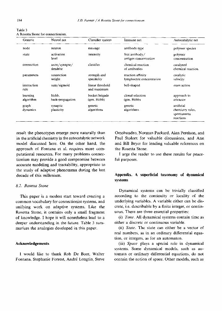
184
Table 3 A Rosetta Stone for connectionism.
J.D. Farmer/A Rosetta Stone for connectionism
Generic Neural net Classifier system Immune net Autocatalytic net
node neuron message antibody type
state activation intensity free antibody/ level antigen concentration
connection axonflsynapse/ classifier chemical reaction dendrite of antibodies
parameters connection strength and reaction affinity weight specificity lymphocyte concentration
interaction sum/sigmoid linear threshold bell-shaped rule and maximum
learning Hcbb, bucket brigade clonal selection algorithm back-propagation (gen. Hcbb) (gen. Hcbb)
graph synaptic genetic genetic dynamics plasticity algorithms algorithms
polymer species
polymer concentration
catalyzed chemical reaction
catalytic velocity
mass action
approach to attractor
artificial chemistry rules, spontaneous reactions
result the phenotypes emerge more naturally than in the artificial chemistry in the autocatalytic network model discussed here. On the other hand, the approach of Fontana et al. requires more com- putational resources. For many problems connec- tionism may provide a good compromise between accurate modeling and tractability, appropriate to the study of adaptive phenomena during the last decade of this millenium.
8.2. Rosetta Stone
This paper is a modest start toward creating a common vocabulary for connectionist systems, and unifying work on adaptive systems. Like the Rosetta Stone, it contains only a small fragment
of knowledge. I hope it will nonetheless lead to a deeper understanding in the future. Table 3 sum- marizes the analogies developed in this paper.
Acknowledgements
I would like to thank Rob De Boer, Walter Fontana, Stephanie Forrest, Andr~ Longtin, Steve
Omohundro, Norman Packard, Alan Perelson, and Paul Stolorz for valuable discussions, and Ann and Bill Beyer for lending valuable references on the Rosetta Stone.
I urge the reader to use these results for peace- ful purposes.
Appendix. A superficial taxonomy of dynamical systems
Dynamical systems can be trivially classified according to the continuity or locality of the underlying variables. A variable either can be dis- crete, i.e. describable by a finite integer, or contin- uous. There are three essential properties:
(i) Time. All dynamical systems contain time as either a discrete or continuous variable.
(ii) State. The state can either be a vector of real numbers, as in an ordinary differential equa- tion, or integers, as for an automaton.
(iii) Space plays a special role in dynamical systems. Some dynamical models, such as au- tomata or ordinary differential equations, do not contain the notion of space. Other models, such as
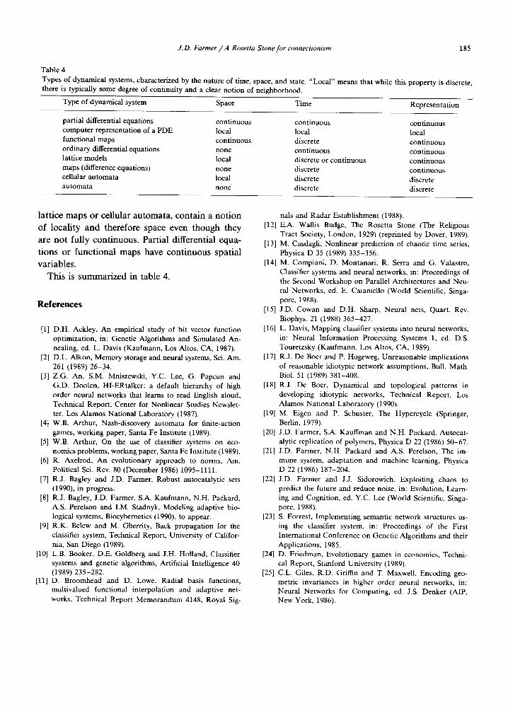
J.D. Farmer/A Rosetta Stone for connectionism
Table 4
Types of dynamical systems, characterized by the nature of time, space, and state. "Local" means that while this there is typically some degree of continuity and a clear notion of neighborhood.
185
property is discrete,
Type of dynamical system Space Time Representation
partial differential equations continuous continuous continuous computer representation of a PDE local local local functional maps continuous discrete continuous ordinary differential equations none continuous continuous lattice models local discrete or continuous continuous maps (difference equations) none discrete continuous cellular automata local discrete discrete automata none discrete discrete
lattice maps or cellular automata, contain a notion of locality and therefore space even though they are not fully continuous. Partial differential equa- tions or functional maps have continuous spatial variables.
This is summarized in table 4.
References
[1] D.H. Ackley, An empirical study of bit vector function optimization, in: Genetic Algorithms and Simulated An- nealing, ed. L. Davis (Kaufmann, Los Altos, CA, 1987).
[2] D.L. Alkon, Memory storage and neural systems, Sci. Am. 261 (1989) 26-34.
[3] Z.G. An, S.M. Mniszewski, Y.C. Lee, G. Papcun and G.D. Doolen, HI-ERtalker: a default hierarchy of high order neural networks that learns to read English aloud, Technical Report, Center for Nonlinear Studies Newslet- ter, Los Alamos National Laboratory (1987).
[4] W.B. Arthur, Nash-discovery automata for finite-action games, working paper, Santa Fe Institute (1989).
[5] W.B. Arthur, On the use of classifier systems on eco- nomics problems, working paper, Santa Fe Institute (1989).
[6] R. Axelrod, An evolutionary approach to norms, Am. Political Sci. Rev. 80 (December 1986) 1095-1111.
[7] R.J. Bagley and J.D. Farmer, Robust autocatalytic sets (1990), in progress.
[8] R.J. Bagley, J.D. Farmer, S.A. Kaufmann, N.H. Packard, A.S. Perelson and I.M. Stadnyk, Modeling adaptive bio- logical systems, Biocybernetics (1990), to appear.
[9] R.K. Belew and M. Gherrity, Back propagation for the classifier system, Technical Report, University of Califor- nia, San Diego (1989).
[10] L.B. Booker, D.E. Goldberg and J.H. Holland, Classifier systems and genetic algorithms, Artificial Intelligence 40 (1989) 235-282.
[11] D. Broomhead and D. Lowe, Radial basis functions, multivalued functional interpolation and adaptive net- works, Technical Report Memorandum 4148, Royal Sig-
nals and Radar Establishment (1988). [12] E.A. Wallis Budge, The Rosetta Stone (The Religious
Tract Society, London, 1929) (reprinted by Dover, 1989). [13] M. Casdagli, Nonlinear prediction of chaotic time series,
Physica D 35 (1989) 335-356. [14] M. Compiani, D. Montanari, R. Serra and G. Valastro,
Classifier systems and neural networks, in: Proceedings of the Second Workshop on Parallel Architectures and Neu- ral Networks, ed. E. Caianiello (World Scientific, Singa- pore, 1988).
[15] J.D. Cowan and D.H. Sharp, Neural nets, Quart. Rev. Biophys. 21 (1988) 365-427.
[16] L. Davis, Mapping classifier systems into neural networks, in: Neural Information Processing Systems 1, ed. D.S. Touretzsky (Kaufmann, Los Altos, CA, 1989).
[17] R.J. De Boer and P. Hogeweg, Unreasonable implications of reasonable idiotypic network assumptions, Bull. Math. Biol. 51 (1989) 381-408.
[18] R.J. De Boer, Dynamical and topological patterns in developing idiotypic networks, Technical Report, Los Alamos National Laboratory (1990).
[19] M. Eigen and P. Schuster, The Hypercycle (Springer, Berlin, 1979).
[20] J.D. Farmer, S.A. Kauffman and N.H. Packard, Autocat- alytic replication of polymers, Physica D 22 (1986) 50-67.
[21] J.D. Farmer, N.H. Packard and A.S. Perelson, The im- mune system, adaptation and machine learning, Physica D 22 (1986) 187-204.
[22] J.D. Farmer and J.J. Sidorowich, Exploiting chaos to predict the future and reduce noise, in: Evolution, Learn- ing and Cognition, ed. Y.C. Lee (World Scientific, Singa- pore, 1988).
[23] S. Forrest, Implementing semantic network structures us- ing the classifier system, in: Proceedings of the First International Conference on Genetic Algorithms and their Applications, 1985.
[24] D. Friedman, Evolutionary games in economics, Techni- cal Report, Stanford University (1989).
[25] C.L. Giles, R.D. Griffin and T. Maxwell, Encoding geo- metric invariances in higher order neural networks, in: Neural Networks for Computing, ed. J.S. Denker (AIP, New York, 1986).

186 J.D. Farmer / A Rosetta Stone for connectionism
[26] S.A. Harp, T. Samad and A Guha, Towards the genetic synthesis of neural networks, in: Proceedings of the Third International Conference on Genetic Algorithms, ed. J.D. Schaffer (Kaufmann, Los Altos, CA, 1989).
[27] J. Hofbauer and K. Sigmund, The Theory of Evolution and Dynamical Systems (Cambridge Univ. Press, Cam- bridge, 1988).
[28] G.W. Hoffmann, A theory of regulation and self-nonself discrimination in an immune network, European J. Im- munol. 5 (1975) 638-647.
[29] G.W. Hoffmann, T.A. Kion, R.B. Forsyth, K.G. Soga and A. Cooper-Willis, The n-dimensional network, in: Theo- retical Immunology, Part II, ed. A.S. Perelson (Santa Fe Institute/Addison-Wesley, Redwood City, CA, 1988).
[30] J. Holland, Escaping brittleness: the possibilities of gen- eral purpose machine learning algorithms applied to paral- lel rule-based systems, in: Machine Learning II, eds. Michalski, Carbonell and Mitchell (Kaufmann, Los Altos, 1986).
[31] J. Holland, K.J. Holyoak, R.F. Nisbett and P.R. Thagard, Induction: Process of Inference, Learning and Discovery (MIT Press, Cambridge, MA, 1986).
[32] J. Hopfield and D.W. Tank, "Neural" computation of decisions in optimization problems, Biol. Cybern. 52 (1985) 141-152.
[33] N.K. Jerne, The immune system, Sci. Am. 229 (1973) 52-60.
[34] N.K. Jerne, Towards a network theory of the immune system, Ann. Immunology (Inst. Pasteur) 125 C (1974) 373-389.
[35] R. Jones, C. Barnes, Y.C. Lee and K. Lee, Fast algorithm for localized prediction, private communication (1989).
[36] S.A. Kauffman, Autocatalytic sets of proteins, J. Theor. Biol. 119 (1986) 1-24.
[37] S.A. Kauffman, Emergent properties in random complex automata, Physica D 10 (1984) 145-156.
[38] S.A. Kauffman, Metabolic stability and epigenesis in ran- domly constructed genetic nets, J. Theor. Biol. 22 (1969) 437.
[39] S.A. Kauffman, Origins of Order, Self-Organization, and Selection in Evolution (Oxford Univ. Press, Oxford, 1990), in press.
[40] C.G. Langton, ed., Artificial Life (Addison-Wesley, Red- wood City, CA 1989).
[41] R. Marimon, E. McGrattan and T.J. Sargeant, Money as a medium of exchange in an economy with artificially intel- ligent agents, Technical Report 89-004, Santa Fe Institute, Santa Fe, NM (1989).
[42] W.S. McCulloch and W. Pitts, A logical calculus of the ideas immanent in nervous activity, Bull. Math. Biophys. 5 (1943) 115-133.
[43] G.F. Miller, P.M. Todd and S.U. Hegde, Designing neural networks using genetic algorithms, in: Proceedings of the Third International Conference on Genetic Algorithms, ed. J.D. Schaffer (Kaufmann, Los Altos, CA, 1989).
[44] J. Miller and S. Forrest, The dynamical behavior of classi- fier systems, in: Proceedings of the Third International
Conference on Genetic Algorithms, ed. J.D. Schaffer (Kaufmann, Los Altos, CA), in press.
[45] S.L. Miller and H.C. Urey, Organic compound synthesis on the primitive earth, Science 130 (1959) 245-251.
[46] D. Montana and L. Davis, Training feedforward neural networks using genetic algorithms, in: Proceedings of the Eleventh International Joint Conference on Artificial In- telligence, 1989.
[47] J. Moody and C. Darken, Learning with localized recep- tive fields, Technical Report, Department of Computer Science, Yale University (1988).
[48] A. Newell, Production systems: models of control struc- tures, in: Visual Information Processing, ed. W.G. Chase (Academic Press, New York, 1973).
[49] J. Pearl, Probabihstic Reasoning in Intelligent Systems: Networks of Plausible Inference (Kaufmann, Los Altos, CA, 1988).
[50] A.S. Perelson, Immune network theory, Immunol. Rev. 110 (1989) 5-36.
[51] A.S. Perelson, Toward a realistic model of the immune system, in: Theoretical Immunology, Part II, ed. A.S. Perelson (Santa Fe Institute/Addison-Wesley, Redwood City, CA, 1988).
[52] E.S. Pichler, J.D. Keeler and J. Ross, Comparison of self-organization and optimization in evolution and neural network models, Technical Report, Chemistry Depart- ment, Stanford University (1989).
[53] F.J. Pineda, Generalization of backpropagation to recur- rent and higher order neural networks, in: Neural Infor- mation Processing Systems, ed. D.Z. Anderson (AIPI New York, 1988).
[54] T. Poggio and F. Girosi, A theory of networks for approx- imation and learning, MIT preprint (1989).
[55] S. Pope, unpublished research. [56] P.H. Richter, A network theory of the immune system,
European J. Immunol. 5 (1975) 350-354. [57] R. Riolo, CFS-C: a package of domain independent sub-
routines for implementing classifier systems in arbitrary, user-defined environments, Technical Report, Logic of Computers Group, University of Michigan (1986).
[58] F. Rosenblatt, The perceptron: a probabilistic model for information storage and organization in the brain, Psycho- logical Rev. 65 (1958) 386.
[59] D. Rummelhart and J. McClelland, Parallel Distributed Processing, Vol 1 (MIT Press, Cambridge, MA, 1986).
[60] A.C. Scott, Neurophysics (Wiley, New York, 1977). [61] L.A. Segel and A.S. Perelson, Shape space analysis of
immune networks, in: Cell to Cell Signalling: From Ex- periments to Theoretical Models, ed. A. Goldbeter (Academic Press, New York, 1989).
[62] T.J. Sejnowski and C.R. Rosenberg, Parallel networks that learn to pronounce English text, Complex Systems 1 (1987) 145-168.
[63] J. Maynard Smith, Evolutionary game theory, Physica D 22 (1986) 43-49.
[64] F.J. Varela, A. Coutinho, B. Dupire and N.N. Vaz, Cogni- tive networks: immune neural and otherwise, in: Theoreti-
J.D. Farmer / A Rosetta Stone for connectionism 187
cal Immunology, Part II, ed. A.S. Perelson (Santa Fe Institute/Addison-Wesley, Redwood City, CA, 1988).
[65] D. Whitley and T. Hanson, Optimizing neural networks using faster, more accurate genetic search, in: Proceedings of the Third International Conference on Genetic Algo- rithms, ed. J.D. Schaffer (Kaufmann, Los Altos, CA, 1989).
[66] S.W. Wilson, Bid competition and specificity reconsid- ered, Complex Systems 2 (1989) 705-723.
[67] S.W. Wilson, Perceptron redux: emergence of structure, Physica D 42 (1990) 249-256, these Proceedings.
[68] D.H. Wolpert, A benchmark for how well neural nets generalize, Biol. Cybern. 61 (1989) 303-313.