NREL is a national laboratory of the U.S. Department of Energy, Office of Energy Efficiency & Renewable Energy, operated by the Alliance for Sustainable Energy, LLC.

Contract No. DE-AC36-08GO28308

The Impact of Financial Structure on the Cost of Solar Energy Michael Mendelsohn, Claire Kreycik, Lori Bird, Paul Schwabe, and Karlynn Cory

Technical Report NREL/TP-6A20-53086 March 2012

NREL is a national laboratory of the U.S. Department of Energy, Office of Energy Efficiency & Renewable Energy, operated by the Alliance for Sustainable Energy, LLC.

National Renewable Energy Laboratory 1617 Cole Boulevard Golden, Colorado 80401 303-275-3000 • www.nrel.gov

Contract No. DE-AC36-08GO28308

The Impact of Financial Structure on the Cost of Solar Energy Michael Mendelsohn, Claire Kreycik, Lori Bird, Paul Schwabe, and Karlynn Cory

Prepared under Task No. SM10.2444

Technical Report NREL/TP-6A20-53086 March 2012

NOTICE

This report was prepared as an account of work sponsored by an agency of the United States government. Neither the United States government nor any agency thereof, nor any of their employees, makes any warranty, express or implied, or assumes any legal liability or responsibility for the accuracy, completeness, or usefulness of any information, apparatus, product, or process disclosed, or represents that its use would not infringe privately owned rights. Reference herein to any specific commercial product, process, or service by trade name, trademark, manufacturer, or otherwise does not necessarily constitute or imply its endorsement, recommendation, or favoring by the United States government or any agency thereof. The views and opinions of authors expressed herein do not necessarily state or reflect those of the United States government or any agency thereof.

Available electronically at http://www.osti.gov/bridge

Available for a processing fee to U.S. Department of Energy and its contractors, in paper, from:

U.S. Department of Energy Office of Scientific and Technical Information P.O. Box 62 Oak Ridge, TN 37831-0062 phone: 865.576.8401 fax: 865.576.5728 email: mailto:reports@adonis.osti.gov

Available for sale to the public, in paper, from:

U.S. Department of Commerce National Technical Information Service 5285 Port Royal Road Springfield, VA 22161 phone: 800.553.6847 fax: 703.605.6900 email: orders@ntis.fedworld.gov online ordering: http://www.ntis.gov/help/ordermethods.aspx

Cover Photos: (left to right) PIX 16416, PIX 17423, PIX 16560, PIX 17613, PIX 17436, PIX 17721

Printed on paper containing at least 50% wastepaper, including 10% post consumer waste.

iii

Acknowledgments

The authors would like to thank Jennifer DeCesaro of the U.S. Department of Energy Solar Technologies Program for her support of this work. The authors would also like to thank the following individuals for providing thoughtful review comments: Daniel Englander of Agile Energy; Matthew Meares of Amonix; Adam Kobos of Stoel Rives; and Craig Turchi and Jeff Logan of NREL. The authors also wish to thank Mary Lukkonen and Linda Huff of NREL for editorial support. The authors are also indebted to the following individuals who provided invaluable insights and perspectives on solar and renewable energy financing terms and issues:

• Mike Niver, SolarCity

• Matthew Meares, Amonix

• Matt Ferguson, Reznick Group

• Joshua Turner and Jordan Roberts, BrightSource Energy

• Daniel Englander, Agile Energy

• John Harper, Birch Tree Capital

• Adam Kobos, Stoel Rives.

iv

Executive Summary

To stimulate investment in renewable energy generation projects, the federal government developed a series of support structures that reduce taxes for eligible investors—the investment tax credit, the production tax credit, and accelerated depreciation. The nature of these tax incentives often requires an outside investor and a complex financial arrangement to allocate risk and reward among the parties. These financial arrangements are generally categorized as "advanced financial structures." Among renewable energy technologies, advanced financial structures were first widely deployed by the wind industry and are now being explored by the solar industry to support significant scale up in project development.1 This report describes four of the most prevalent financial structures used by the renewable sector and evaluates the impact of financial structure on energy costs for utility-scale solar projects that use photovoltaic and concentrating solar power technologies.

A critical aspect of the analysis is the input assumptions, including the cost to install each technology, the costs and terms of financial capital relevant to the technology and financial structure assessed, and the operating costs of each technology. To determine reasonable inputs, the authors conducted a series of interviews with industry experts, reviewed several sources in the current literature, and relied on the default values from the System Advisor Model that was employed in this analysis, which were, in turn, guided by the industry expertise of its developers.

The analysis determined that financial structures that include project-level debt generally yield a lower levelized cost of energy (LCOE) compared to those that rely purely on equity capital, although in practice raising debt at the project level can be difficult, particularly for developers without sizable balance sheets and a strong history of development experience. Other insights from the analysis include:

• Debt associated with the loan guarantee program can reduce LCOE by approximately 20%, and possibly more, depending on the quantity of debt the project is allowed to take on.

• Certain financial experts expect "tax equity" capital—incorporated to maximize the use of federal tax credits and depreciation benefits—to increase in cost by 200 to 400 basis points (bp) (or 2%–4%) due to the termination of the current 1603 Treasury grant program at the end of 2011.2 Such an increase in the cost of tax equity is projected to raise the LCOE from utility-scale solar projects by 3%–20%.

• The cost of tax equity is particularly critical in all-equity financial structures and can have a significant impact on the cost of energy produced. Even more important in all-equity financial structures, the internal rate of return (IRR) target year—the project year in which the tax equity investor is expected to earn the pre-negotiated return—can have a very large impact on the resulting cost of energy. Delaying the IRR target year, for example, from year eight of the project to year nine, can improve the LCOE by 7%–27%, depending on the technology and financial structure employed.

1 Lease structures have been used by the solar industry under earlier investment tax credits. 2 See Section 1603 of Division B of the American Recovery and Reinvestment Act of 2009, as amended.

v

• Development and operational experience is projected to lead to further financial structure innovation and reduction in required investment returns for various sources of financial capital.

vi

Table of Contents List of Figures ........................................................................................................................................... vii List of Tables ............................................................................................................................................. vii 1 Introduction ........................................................................................................................................... 1 2 Background on Financing Structures ................................................................................................ 4

2.1 Single Owner .......................................................................................................................5 2.2 All-Equity Partnership Flip ..................................................................................................6 2.3 Leveraged Partnership Flip ..................................................................................................8 2.4 Sale Leaseback .....................................................................................................................9

3 Selection of Financing Structures in the Marketplace ................................................................... 11 4 Analysis and SAM Model Overview .................................................................................................. 14 5 Technology and Economic Assumptions ........................................................................................ 15 6 Financial Analysis Methodology ....................................................................................................... 17

6.1 Reference Cases .................................................................................................................17 7 Results ................................................................................................................................................. 20

7.1 Reference Case...................................................................................................................20 7.2 Scenario and Sensitivity Analysis ......................................................................................21

7.2.1 Single Variable Scenarios .........................................................................................22 7.2.2 Low and High Financing Cost Scenarios..................................................................24

8 Conclusion .......................................................................................................................................... 27 References ................................................................................................................................................. 29 Appendix A. Tables of Results ................................................................................................................ 30

vii

List of Figures Figure 1. U.S. utility-scale solar projects currently under development ............................................... 2 Figure 2. Single owner example structure ................................................................................................ 5 Figure 3. All-equity partnership flip example structure and allocations ............................................... 7 Figure 4. Leveraged partnership-flip example structure and allocations ............................................. 9 Figure 5. Sale leaseback example structure .......................................................................................... 10 Figure 6. Financial structure impact on CSP and PV real LCOE (reference case) ............................. 20 Figure 7. LCOE spreads between low and high cases for PV, CSP-Trough, and CSP-Tower .......... 26

List of Tables Table 1. Summary of Key Elements of Financing Structures (as modeled for analysis) .................... 4 Table 2. Power Plant Cost Assumptions ................................................................................................ 15 Table 3. Key Financing Variables by Financial Structure – PV Reference Case ................................ 18 Table 4. Key Financing Variables by Financial Structure – CSP Reference Case ............................. 19 Table 5. Comparison of Real LCOE, Nominal LCOE, and First-Year PPA Price for a Theoretical PV

Plant ($/kWh) .............................................................................................................................. 21 Table 6. LCOE Impact of Loan Guarantee Financing Case – PV, CSP-Trough, and CSP-Tower

($/kWh) ........................................................................................................................................ 22 Table 7. LCOE Impact of Altered Target Year for PV ($/kWh Real) ...................................................... 23 Table 8. LCOE Impact of Increased Cost of Equity (PV only) ($/kWh) ................................................ 24 Table 9. Modified Inputs for Low and High Scenarios (for all technologies) ...................................... 25 Table A-1. Reference Case Results ($/kWh) ........................................................................................... 30 Table A-2. Low Case Results ($/kWh) ..................................................................................................... 31 Table A-3. High Case Results ($/kWh) .................................................................................................... 32

1

1 Introduction

The U.S. government has established several mechanisms to support investment in renewable energy generation facilities through the tax code. The two most critical support structures offered by the federal government are (1) investment or production tax credits (ITC or PTC), and (2) an accelerated depreciation schedule for renewable energy projects known as the Modified Accelerated Cost Recovery System (MACRS) and a “bonus” depreciation that allows for additional acceleration of the tax benefits to investors.3 Both the ITC/PTC and MACRS mechanisms can benefit the project by reducing the taxes payable, thereby improving the economic performance of the project. In total, the economic benefit of the federal tax incentives can represent roughly 50%–60% of the installed cost of the solar project (Bolinger 2009). In recent years, there has also been a cash grant available through the Treasury 1603 program in lieu of the ITC, which expired at the end of 2011.

However, renewable energy project developers typically do not have sufficient taxable income to take full advantage of the tax incentives directly.4 Accordingly, renewable energy project developers have implemented a wide array of complex financing structures with specialized “tax equity investors” (typically large investment banks or insurance companies) that have sufficient taxable income from other business activities and expertise to take advantage of the tax benefits.

These financial structures, such as "partnership flips" and various lease structures, have been instrumental in the maturation of the wind industry. As the photovoltaic (PV) and concentrating solar power (CSP) industries continue to develop utility-scale facilities, advanced financial structures are likely to play an increasingly important role in the allocation of risk and reward among different investor classes.

According to the National Renewable Energy Laboratory’s (NREL’s) database of utility-scale projects of 5 megawatts (MW) or greater, more than 16,000 MW are currently under development and hold a power purchase agreement (PPA) with a utility or are under development by a utility (see Figure 1).

3 The federal ITC enables developers to obtain a 30% tax credit for expenditures associated with installing qualifying renewable energy facilities installed by the end of 2016. Facilities qualifying for the 30% ITC include solar, small wind, and fuel cells. The PTC is a federal tax credit of $0.022/kilowatt-hour (kWh) inflation adjusted for the first 10 years of generation from qualifying renewable energy facilities. The PTC is available for wind project through the end of 2012 and for other qualifying technologies such as biomass, geothermal, and marine and hydrokinetic resources through 2013. The PTC is not applicable to solar projects. The MACRS depreciation incentive allows projects to depreciate projects over an accelerated five-year schedule. A 50% first year bonus depreciation provision is currently available through the end of 2012. For more information on these tax incentives, see the Database of State Incentives for Renewable Energy (DSIRE) at http://dsireusa.org/incentives/incentive.cfm?Incentive_Code=US06F&re=1&ee=1. Accessed December 13, 2011. 4 Because the cash grants are scheduled to expire, this analysis focuses on incentives that require tax equity investment to take full advantage of the tax incentives.

2

Figure 1. U.S. utility-scale solar projects currently under development

According to a study by the Lawrence Berkeley National Laboratory (LBNL), the cost of wind energy can be highly influenced by the financing structure utilized, ranging from $48 per megawatt-hour (MWh) to $63/MWh for a hypothetical project (Harper et al. 2007). The authors found the variation in costs to result primarily from (1) financing-related transaction costs, (2) assumptions about internal rate of return for tax and equity investors, and (3) the relative terms of each structure including the level of equity versus debt. Factors that were found to be important in selecting financing structures were: simplicity, standardization, and speed of the financing process. While financial structures utilizing project-level debt were determined to have a lower cost of energy in analytical models, the use of debt was perceived by actual equity investors as expensive to implement (i.e., requiring costly due diligence), complex, and leading to a loss of control (Harper et al. 2007).

The purpose of this analysis is to examine the effects of different financial structures on the cost of energy from PV and CSP plants [with differentiation between parabolic-trough CSP (CSP–Trough) and power-tower CSP (CSP–Tower) technologies]. The analysis relies on modeling results from the System Advisor Model (SAM),5 developed by NREL, in collaboration with Sandia National Laboratories (SNL) and in partnership with the U.S. Department of Energy (DOE) Solar Energy Technologies Program. In early 2011, NREL added the capability to assess complex financial structures to SAM (details provided in text box on page 17).

This study examines the levelized cost of energy (LCOE) impact due to financial structure and terms for CSP and PV technologies. The report first describes in detail four commonly used

5 SAM is available at https://www.nrel.gov/analysis/sam/. Accessed September 26, 2011.

3

financial structures—single owner, all-equity partnership flip, leveraged partnership flip, and sale leaseback—and their use in the solar industry. Next it presents results from the SAM model comparing the LCOE for CSP and PV technologies under the four different financing structures. The assumptions used in the modeling are informed by interviews with renewable energy industry financing experts and relevant literature. The study then examines the sensitivity of the LCOE to changes in key financial variables, including tax equity returns, interest rates, and the duration of partnership flips. Finally, conclusions are offered based on the modeling results and interviews with financial experts.

This report is one in a series of three reports on utility-scale solar installation in the United States. The other reports provide (1) a primer on utility-scale solar technologies and market activities, and (2) an overview of the policies that support financing of utility-scale solar systems.

4

2 Background on Financing Structures

This analysis focuses on four commonly used financial structures: single owner, all-equity partnership flip, leveraged partnership flip, and sale leaseback. Innumerable variations on these structures can be applied depending on the risk appetites and reward expectations of the parties involved, including allocation of tax and cash benefits, buyout provisions during set periods along the project life, and default allocation of risk to parties. The following background information on these structures derives primarily from two sources: Wind Project Financing Structures: A Review and Comparative Analysis (Harper et al. 2007) and Renewable Energy Project Financing: Impacts of the Financial Crisis and Federal Legislation (Schwabe et al. 2009). Other sources are cited separately.

The key elements of the four financing structures are summarized below and in Table 1.

Table 1. Summary of Key Elements of Financing Structures (as modeled for analysis)6

Single Owner All-Equity

Partnership Flip Leveraged Partnership Flip

Sale Leaseback

Equity Owners

Developer

(third party if sold)

Tax investor;

developer

Tax investor;

developer

Tax investor (lessor)

Project Debt

Yes (owner choice)

None Yes None

Return Target

Owner After-Tax IRR

Tax investor after-tax IRR (flip target)

Tax investor after-tax IRR (Flip Target)

Lessor after-tax IRR

Cash Sharing

Owner: 100% of project cash

Pre-Flip: all to tax investor after developer cost recovery;

Post-Flip: primarily to developer

Pre-Flip: Proportional to investment after developer cost recovery;

Post-Flip: Primarily Developer

Lessor: Receives lease payment;

Lessee: Receives operating budget, project margin

Tax Benefit Sharing

Owner: 100% of project tax benefits

Pre-Flip: primarily tax investor;

Post-Flip: primarily developer

Pre-Flip: primarily tax investor;

Post-Flip: primarily developer

Lessor and lessee different taxable incomes;

ITC & depreciation to lessor

Sources: Karcher et al. 2010; SAM User Guide 2011 6 This table does not represent all of the projects using financial structure in today’s market. Actual market projects may have very unique features.

5

2.1 Single Owner The single owner structure involves one project owner, which can be either the project sponsor (developer) or a large taxable entity that has purchased the project from a developer. The single owner receives all of the cash and tax benefits (see Figure 2).7 Generally, an entity that enters into a single-owner structure for a renewable energy generation project has the ability to use all of the tax benefits from the project.8

The single owner may or may not utilize project-level debt to finance the facility. The analysis contained herein assumes project-level debt was employed for the single-owner structure.

Figure 2. Single owner example structure

Source: Harper et al. 2007

The developer or investor often creates a special purpose entity for the project assets and pays the project’s capital costs with funds from other operations. All of the project cash flows, tax incentives, and depreciation benefits remain with the owner. This structure is widely used for renewable energy projects and represents one of the simplest methods of owning and operating a project. There is no third-party equity requirement and there are no flip targets. The owner may acquire project-level debt or obtain financing at the company or parent level. The original SAM "independent power producer" (IPP) financial model follows this structure.

7 Shaded areas represent disbursement of benefits and assumed allocations among investors. 8 Note that a single owner is usually not a utility due to Internal Revenue Service normalization rules (see Scharfenberger 2011).

Senior Lender(if obtained)

Owner(100% of equity)

Project Company(equity + PPA/cash debt)

Power (and REC) Sales

Cash Revenue Investment Tax Credit/Cash Grant

lessOperatingExpenses

lessDebt Service

lessTax-Deductible Expenses

(including MACRS and interest on debt)

equalsTaxable Losses/Income

(which result inTax Benefits/Liabilities)

equalsDistributable Cash

100%

100%

Federal Incentive

100%

6

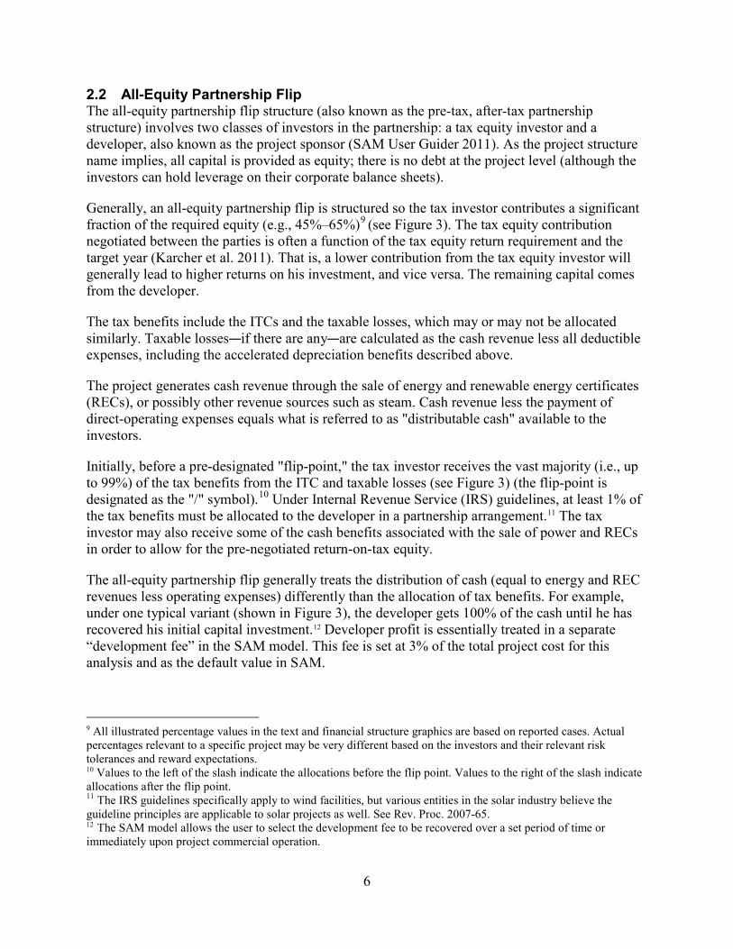
2.2 All-Equity Partnership Flip The all-equity partnership flip structure (also known as the pre-tax, after-tax partnership structure) involves two classes of investors in the partnership: a tax equity investor and a developer, also known as the project sponsor (SAM User Guider 2011). As the project structure name implies, all capital is provided as equity; there is no debt at the project level (although the investors can hold leverage on their corporate balance sheets).

Generally, an all-equity partnership flip is structured so the tax investor contributes a significant fraction of the required equity (e.g., 45%–65%)9 (see Figure 3). The tax equity contribution negotiated between the parties is often a function of the tax equity return requirement and the target year (Karcher et al. 2011). That is, a lower contribution from the tax equity investor will generally lead to higher returns on his investment, and vice versa. The remaining capital comes from the developer.

The tax benefits include the ITCs and the taxable losses, which may or may not be allocated similarly. Taxable losses—if there are any—are calculated as the cash revenue less all deductible expenses, including the accelerated depreciation benefits described above.

The project generates cash revenue through the sale of energy and renewable energy certificates (RECs), or possibly other revenue sources such as steam. Cash revenue less the payment of direct-operating expenses equals what is referred to as "distributable cash" available to the investors.

Initially, before a pre-designated "flip-point," the tax investor receives the vast majority (i.e., up to 99%) of the tax benefits from the ITC and taxable losses (see Figure 3) (the flip-point is designated as the "/" symbol).10 Under Internal Revenue Service (IRS) guidelines, at least 1% of the tax benefits must be allocated to the developer in a partnership arrangement.11 The tax investor may also receive some of the cash benefits associated with the sale of power and RECs in order to allow for the pre-negotiated return-on-tax equity.

The all-equity partnership flip generally treats the distribution of cash (equal to energy and REC revenues less operating expenses) differently than the allocation of tax benefits. For example, under one typical variant (shown in Figure 3), the developer gets 100% of the cash until he has recovered his initial capital investment.12 Developer profit is essentially treated in a separate “development fee” in the SAM model. This fee is set at 3% of the total project cost for this analysis and as the default value in SAM.

9 All illustrated percentage values in the text and financial structure graphics are based on reported cases. Actual percentages relevant to a specific project may be very different based on the investors and their relevant risk tolerances and reward expectations. 10 Values to the left of the slash indicate the allocations before the flip point. Values to the right of the slash indicate allocations after the flip point. 11 The IRS guidelines specifically apply to wind facilities, but various entities in the solar industry believe the guideline principles are applicable to solar projects as well. See Rev. Proc. 2007-65. 12 The SAM model allows the user to select the development fee to be recovered over a set period of time or immediately upon project commercial operation.

7

After the developer recovers its initial investment (designated as the first slash in the bottom boxes of Figure 3), the developer receives 1% of the distributable cash. The tax equity investor receives 99%. After the flip point is reached and when the tax equity investor’s return hits the pre-negotiated target (designated as the second slash in the same boxes), the allocation of cash will change again. This analysis assumes the developer gets 10% of the distributable cash and the tax equity investor 90% after the flip point, also the default values in SAM.

Figure 3. All-equity partnership flip example structure and allocations Source: Adapted from Karcher et al. 2010

The project will reach the designated flip point once the total return (from tax and cash benefits) earned by the tax equity investor reaches a pre-negotiated internal rate of return (IRR). After the flip point is reached, the benefit streams are reallocated among the investors according to the pre-designed arrangement. The flip point is often referred to as the IRR "target year."

Typically, the allocations and equity contributions are designed so that the flip point occurs after the tax benefits have been fully realized and the five-year ITC “recapture” period has expired. During the recapture period, the IRS requires investors that utilize tax benefits to hold onto the assets or risk losing all tax benefits enjoyed since commercial operation began.

Tax Investor(60% of equity)

Developer(40% of equity)

Project Company(100% equity)

Power (and REC) Sales

Cash Revenue Investment Tax Credit/Cash Grant

lessOperatingExpenses

lessTax-Deductible Expenses

(including MACRS)

equalsTaxable Losses/Gains

(which result inTax Benefits/Liabilities)

equalsDistributable Cash

99% / 90%

99% / 90% 1% / 10%

100% / 0% / 10% 0% / 100% / 90%

1% / 10%

Federal Incentive

8

Some all-equity partnership flip structures utilize more flip points and associated reallocations of project benefits than represented in Figure 3, depending on the desires of the investors.13

2.3 Leveraged Partnership Flip The leveraged partnership-flip structure is similar to the all-equity partnership flip but also includes project-level debt. The fraction of debt is determined by the debt terms, the cash generated by the project, and the limits placed by the lending institution. The loan is often sized such that it can be repaid from project cash flow and secured by the project’s assets. The SAM model calculates the fraction of debt as the maximum allowable level given a user-defined debt-service coverage ratio (DSCR). The DSCR represents the additional cash available to service the debt.

Typically, in a leveraged partnership flip, the tax investor contributes virtually all of the equity required after the debt is secured and receives a pro rata allocation (i.e., proportional to its equity contribution) of both cash and tax benefits until it has achieved the pre-negotiated flip target. The developer generally makes a very small equity investment (e.g., 2% of the total equity invested) (see Figure 4).

Like the all-equity partnership flip, the benefit allocations within the leveraged partnership flip are usually designed to provide a flip point within years six to nine of the solar project’s life. After the flip point is reached, the benefits are reallocated to provide the project developer the vast majority (e.g., 90%) of the project cash and remaining tax benefits. As with the equity flip, the post-flip allocations are determined to allow the tax investor to achieve a specific 20-year IRR. The equity contributions and allocation fractions can vary substantially by project. Because the lenders have the first lien on project assets, the equity IRR requirements are higher than with an all-equity partnership flip.

13 The SAM model employed for this analysis is only capable of examining flip structures with a single-flip point.

9

Figure 4. Leveraged partnership-flip example structure and allocations Source: Adapted from Harper et al. 2010

2.4 Sale Leaseback The sale leaseback structure involves a tax equity investor who purchases the project from the developer and then leases it back (SAM User Guide 2011). In this structure, the tax investor (the lessor) leases the facility back to the developer (the lessee) and receives lease payments. The tax investor holds all of the tax credits and depreciation benefits from the project (see Figure 5).

The lessee operates the project and receives revenues from sales of electricity. The lessee also typically retains excess cash flow after operating costs and lease payments are made, which provides an incentive for the developer to operate the project efficiently.

Unlike the flip structures, under the sale leaseback structure, the tax equity investor and developer each have their own taxable income and project cash flows; there is no revenue sharing. However, there are cash flows being exchanged between the two parties as a result of the lease arrangement. The return target is the tax investor’s IRR requirement at a given point in time, typically the end of the lease term.

Senior Lender

Tax Investor(98% of equity)

Developer(2% of equity)

Project Company(equity + PPA/cash debt)

Power (and REC) Sales

Cash Revenue Investment Tax Credit/Cash Grant

lessOperatingExpenses

lessDebt Service

lessTax-Deductible Expenses

(including MACRS and interest on debt)

equalsTaxable Losses/Income

(which result inTax Benefits/Liabilities)

equalsDistributable Cash

98% / 10%

98% / 10% 2% / 90%

2% / 90% 98% / 10%

2% / 90%

Federal Incentive

10

Figure 5. Sale leaseback example structure Source: Karcher et al. 2010

Usually, the purchase price is based on the underlying project value relative to the tax-investor-required rate of return and known revenues, such as a signed PPA. The lease payments are sized based on a pre-defined lease coverage ratio to ensure there is adequate cash in the project to cover the lease payments. The purchase price of the project is based on the present value of lease payments, tax incentives, and depreciation, and is usually supported by an appraisal.

Developer Tax Investor(100% of equity)

ProjectOwned by Tax Investor; leased by Developer

Power (and REC) Sales

Cash Revenue ITC or Cash Grant

lessOperating Expenses

(including lease payment)

MACRS Depreciation DeductionsequalsDistributable Cash

100%

Federal Incentive

100%

100%

Lease Agreement

Sale of Asset

Lease Payment

11

3 Selection of Financing Structures in the Marketplace

The authors conducted a series of interviews with the following industry experts selected for their knowledge of financial structures and large-scale solar development: Matthew Meares, Amonix; Matt Ferguson, Reznick Group; Joshua Turner and Jordan Roberts, BrightSource Energy; Daniel Englander, Agile Energy; John Harper, Birch Tree Capital; Adam Kobos, Stoel Rives; and Mike Niver, SolarCity. Interview topics ranged from the cost and availability of various sources of capital to pros and cons of specific financial structures.

The selection of financing structures for any particular project is based on a variety of factors. Expert interviews suggest that these factors include: project size, experience and comfort with the structure, the strength of the developer’s balance sheet, the ability to use tax credits, and the investor’s risk tolerance and preferences. Harper et al. (2007) also found simplicity, standardization, and speed of the financing process to be important in selecting financing structures.

Interviews also indicated that, because tax equity is in such high demand by a wide array of projects both inside and outside the renewable energy industry, the tax equity investor generally dictates many of the terms of the agreement including the financial structure selected. The tax equity market was often categorized by interview candidates as quite constrained and difficult to access, particularly for projects proposed by newer developers or those employing technologies without significant operational experience.

Tax equity investors frequently specialize in a particular structure due to experience and general comfort with the associated risks. Interviews with developers indicate that they will utilize a variety of structures, the final selection generally depending on tax investor preference and the expected risk/return tradeoff of the offers. The investors in these projects may regard the tax credit incentives—ITC, PTC, and cash grant—differently due to their variable impacts on LCOE and return expectations. Whether the incentive is production-based or investment-based impacts the present value of cash flow to equity. The tax equity investor may have the final say in which financing structure is used.

All interviewees advised developers to evaluate their projects under a range of potential financial structures before setting the PPA with the utility or other off-taker. The reality of the financial structure required by the tax investor may force the PPA to be framed in a certain way or cause higher expenses than assumed by developers when setting the PPA.

Lease structures or master lease agreements, which can be used to streamline a large number of projects, are common for PV in particular. One developer indicated he does not use flip structures because he does not have the tax appetite to take even a small amount of tax credits, while another indicated that some investors are not able to enter into partnership deals because of limitations in their charters. Flip structures can also be challenging for smaller utility-scale projects because of the cost and complexity of structuring the partnership. Also, there is greater uncertainty in the timing of payment with flip structures than with lease structures. Another developer indicated that flip structures are the most forgiving and the easiest to administer, with the fewest number of steps to undertake. The choice of structure can also be influenced by the developer’s interest in monetizing cash flows. Accounting treatment of revenues and losses can

12

be vastly different between structures, which may result in the developer or equity investor preferring one structure or another.

One interviewee in the PV industry indicated that, presently, it is difficult to negotiate debt when tax equity investors are involved, due to issues of forbearance and ownership.14 Forbearance is a special agreement between the lender and the borrower to delay a foreclosure. While the tax equity investor is the owner of the project, senior debt would have a first lien on the assets in the case of bankruptcy. If a project defaults on its debt payments and the lender places a lien on the project, the owner may need to forfeit the tax incentives.

The details of the forbearance and ownership are very complicated, often requiring extensive legal review. For that reason, debt is generally only available at the project level to very large projects or a portfolio of projects. One interviewee indicated that debt lenders prefer to be engaged only in projects of $25 million to $50 million or larger. This is generally true whether the project incorporates direct ownership (i.e., single owner structure), a partnership flip, or a lease structure of some kind (referred to as a levered lease transaction). The only CSP-Trough facility completed of late (the Nevada Solar One Plant developed in 2007) utilized a levered lease transaction.

Joint ventures (also known as strategic partnerships) may be employed in some circumstances in lieu of a partnership flip. In contrast to a partnership flip, a joint venture represents a business venture with equity partners that take pro rata allocations of cash and tax benefits consistent with their investments in the joint venture and are not expected to exit the project after hitting a specified project return.15 Interviewees indicated that joint ventures may be used when tax equity investors perceive that there is too much risk to invest or when a joint venture provides synergies or other benefits.

In one example of a recent joint venture, BrightSource Energy has raised equity at the corporate level and partnered with companies, including NRG Energy and Google, on the CSP-Tower project, Ivanpah Solar Electric Generating System (BrightSource 2011). However, the financial structure of the Ivanpah facility could still evolve as the parties weigh their options during or after construction. Overall, there is minimal market data to assess the preferred financial structure of the market to develop CSP facilities. As mentioned, only one CSP-Trough project was built in the recent past, and no CSP-Tower facilities have been completed recently in the United States.

Project structures frequently allow the developer, or sponsor, to re-purchase the project from the tax equity investor during various intervals along the project life. These repurchase options can provide significant value to the sponsor but are often based on qualitative inputs (e.g., “it’s

14 Because of their capital-intensive nature, renewable energy projects are typically financed using non-recourse, or project, financing under which a special purpose entity is created to shield the sponsor from the detrimental effects of project failure. Under non-recourse financing, the project assets are paid for entirely from project cash flow, not the sponsor’s balance sheet. In contrast, under a corporate finance structure, loans are secured from the general assets or creditworthiness of the project sponsors. 15 There is no specific method to assess joint ventures in the SAM model. Instead, one could utilize the single- owner structure and input the weighted average cost of equity among the joint venture parties as the required return on equity.

13

consistent with their business model”) or require nuanced modeling beyond the capabilities of NREL’s SAM model. Accordingly, the analysis in the following section ignored issues of repurchase or buyout.

14

4 Analysis and SAM Model Overview

This analysis examines the impact of financial structure on energy costs for large-scale solar PV and CSP plants, using the metric of real LCOE. Simply stated, LCOE is a discounted measure of the costs of building and maintaining an electric generating system divided by the discounted amount of energy produced over the analysis period. Both direct expenditures on the generating system and indirect costs, such as transaction costs, returns, and interest rates, contribute to the LCOE.

To complete this analysis, NREL employed the pro forma financial cash flow model that has been integrated into the SAM model to calculate the LCOE and other metrics under the four financial structures discussed above.16 SAM allows users to investigate the impact on LCOE (among other output variables) of variations in project location and physical characteristics, technology performance and cost, and project financing parameters. The authors developed model input assumptions based on market intelligence gathered via the interview process, current literature on the topic, and the default values embedded in the SAM model (also developed by research and industry experts). See Financial Analysis Methodology below.

SAM’s pro forma financial model includes a representative template for each of the project finance structures examined, which is a new feature not included in earlier versions of the model (see text box for differences between the new and old version of SAM).17 For each of the Advanced Utility IPP financing structures, the model incorporates the assumed rates of return by the developer or tax equity investor, the equity contribution ratios, and the cash and tax benefits allocations, and then solves for the LCOE needed to satisfy those input assumptions.18 The model also includes a wide array of input assumptions associated with power production, installed costs, and facility operations and maintenance (O&M).

16 The analysis was conducted using SAM Version 2011.6.30. 17 The SAM User Guide (Gilman 2011) provides more information about the model and its historical development. 18 The model is not designed to provide a bankable pro forma. The pro forma is an annual model, as opposed to a quarterly or monthly model generally required of banking institutions.

15

5 Technology and Economic Assumptions

This analysis examines the LCOE of utility-scale CSP-Trough and CSP-Tower plants (100 MW nameplate capacity) and PV projects (20 MW-direct current nameplate capacity) using the four financial structures described above. The hypothetical plants are sited in Blythe, California (for CSP-Trough and CSP-Tower), and Phoenix, Arizona (for PV).

Table 2. Power Plant Cost Assumptions

Primary Result CSP-Trough CSP-Tower PV

Project Size (MW) 100 100 20

Installed Cost ($/watt)* $7.50 $6.05 $4.30

Capacity Factor 41% 42% 26%

Generation (Annual MWh) 357,587 367,769 22,348

Fixed O&M $70/kW-year $70/kW-year $10/kW-year

Variable O&M $3/MWh $3/MWh -

*The installed cost is calculated as the “overnight” installed cost, and represents all fixed costs but excludes interest during construction and other financing costs.

Table 2 summarizes the key cost and performance variables assumed in the analysis. These values are the default inputs for SAM at the time of the model runs, and are only intended to be generally representative of project costs. The PV cases assume $4.30/watt (W) fully installed ($86 million total) and incur fixed O&M expenses of $10/kW-year. The PV cases also assume single-axis tracking and a 78% direct current to alternating current derate factor. The analysis assumed CSP-Trough and CSP-Tower systems had installed costs of $7.50/W and $6.05/W, respectively. Fixed O&M costs for CSP technologies are assumed to be $70/kW-year and variable O&M costs are assumed to be $3/MWh.

For all cases, a 35% federal tax rate, 7% state tax rate, and a 5% sales tax was applied. Ongoing expenses were inflated at a rate of 2.5% per year. Annual insurance costs were set at 0.5% of initial capital costs. All cases also assumed a 30% ITC and MACRS depreciation with 50% bonus depreciation.

No other incentive structures, such as REC payments, were assumed available. All cases were modeled for 25 years and on the assumption that the developer does not exercise its option to purchase the investor’s interest in the project.

16

Power production is calculated via SAM. All other performance variables are based on SAM model defaults (version 2011-06-30). A detailed description of the model’s input assumptions and default values is provided in the SAM financials user guide (Gilman 2011).

SAM’s Original IPP Model Versus New Advanced IPP Models

The new financial structures incorporated in SAM version 2011-06-30 are referred to as Advanced Utility IPP options. The prior versions of SAM included three IPP modules relevant to utility-scale projects, which are now rolled into a single Utility IPP case.

There are a number of differences between the original Utility IPP model and the new Advanced Utility IPP options. The Utility IPP model can be considered a simplified version of the current “Single Owner” model, which is included within the Advanced Utility IPP options. However, the two cases may not provide equivalent results for what appears to be the same project due to unique treatment of a few input variables.

The following elements are new to the Advanced Utility IPP models:

• Reserve accounts for debt service and working capital – Reserve accounts are generally required by lenders and investors to improve security of their investments and represent an important cost of financing.

• Sculpted debt – Allows specific year-to-year debt repayment based on the annual project cash flows. The quantity of debt, or debt fraction, is calculated as the maximum that can be loaned to the project given a user-defined constant debt service coverage ratio (DSCR). In contrast, the historic Utility IPP model allowed users to specify a debt fraction and a mortgage-style debt (equal annual payments).

• Developer fee – The Advanced IPP models allow the user to define a developer fee that can be paid upon project commercial operation or from cash flows over a specified time period. The original IPP model does not allow for payment of a development fee.

• MACRS depreciation schedules – The original Utility IPP model included the mid-quarter MACRS schedules. Although the mid-quarter convention can apply to a solar facility depending on the facts and circumstances, mid-quarter schedules cannot be accurately modeled in an annual forecasting tool such as SAM. The feature was removed in the new version of SAM for all IPP cases. Mid-year MACRS schedules (shown in SAM as “5-yr MACRS”) are now the default values and were applied for all cases in this analysis.

• Change in property tax accounting – The original Utility IPP model included default values that projected increasing real estate values and tax increases over time. The Advanced IPP model includes default inputs based on declining real estate values for tax purposes consistent with common property tax valuation practices.

• Financial closing costs – The Advanced Utility IPP models include cost components associated with the acquisition of financial capital, including equity-closing costs and debt-closing costs. The original Utility IPP model did not include these inputs.

17

6 Financial Analysis Methodology

To estimate the relative impacts of financing variables on the resulting cost of solar energy, both single variable sensitivities and scenarios were developed and compared to reference scenarios. Input values for reference and alternative scenarios were chosen based on multiple sources, including:

• Default values within the SAM Advanced Utility IPP models

• Interviews with a number of industry experts experienced with project development and underwriting

• 2010 Mintz Levin report, Renewable Energy Project Finance in the U.S.: An Overview and Midterm Outlook, which provides technology-specific debt and equity returns.

6.1 Reference Cases Tables 3 and 4 present the financing variables used in the analysis for PV and CSP, respectively. One interviewee indicated that the interest rate might be 100 basis points higher for CSP-Tower systems because of the greater technology risk. Accordingly, this incremental return was incorporated in the assumed cost of debt and equity. Also, interviewees indicated that, except for small differences in DSCR, financial variables would not differ significantly for cadmium telluride thin film—the primary commercially available thin-film technology utilized in utility-scale installations at present—and crystalline PV technologies. The analysis did not consider financing costs for technologies not currently under development due to the necessary speculation of input assumptions.

For both PV and CSP, the partnership-flip structures were assumed to have an IRR target of year nine (i.e., the project’s tax investors would reach their target IRRs in year nine of the project if the cash and tax benefits were realized as projected). Equity target returns for PV plants were assumed to be 9% and 11% for the all-equity and leveraged partnership flips, respectively. The equity returns for the leveraged partnership-flip structure are higher because the structure includes a creditor who retains first lien on the project’s cash; the tax investor is assumed to require a higher yield because of this added risk.19 Interviews and other resources indicate that those spreads are approximately two percentage points (200 basis points). For CSP technologies, the target returns are assumed to be higher due to technology risk given that only a small number of projects have been installed in the United States: 12% for all-equity flips and 14% for a leveraged flip (Mintz Levin 2010). However, interviewees indicated that there is no real market experience on which to base these rates.

For structures that allow for project-level debt, including the leveraged partnership flip and single-owner structures, key analysis inputs include the debt interest rate, term, and fees relevant to acquiring the debt instruments. The PV reference case debt rate is assumed to be 7% for 18 years, while the CSP debt rate modeled is 8% for 18 years. Other primary financial inputs to 19 Structures with debt carry a greater default risk for the tax equity investor because the project’s debt lenders get priority rights in the case of project default. Therefore, the tax equity investor in the debt-leveraged structures requires a higher target IRR relative to the all-equity financing structure, which compensates for their increased risk exposure (Cory and Schwabe 2009).

18

the structural analysis include the equity closing costs, development fees, and project benefit allocations.

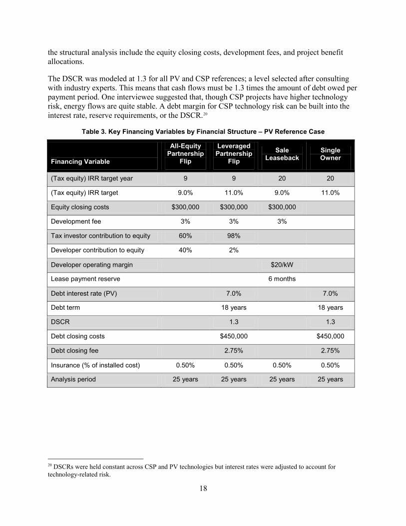
The DSCR was modeled at 1.3 for all PV and CSP references; a level selected after consulting with industry experts. This means that cash flows must be 1.3 times the amount of debt owed per payment period. One interviewee suggested that, though CSP projects have higher technology risk, energy flows are quite stable. A debt margin for CSP technology risk can be built into the interest rate, reserve requirements, or the DSCR.20

Table 3. Key Financing Variables by Financial Structure – PV Reference Case

Financing Variable

All-Equity Partnership

Flip

Leveraged Partnership

Flip

Sale Leaseback

Single Owner

(Tax equity) IRR target year 9 9 20 20

(Tax equity) IRR target 9.0% 11.0% 9.0% 11.0%

Equity closing costs $300,000 $300,000 $300,000

Development fee 3% 3% 3%

Tax investor contribution to equity 60% 98%

Developer contribution to equity 40% 2%

Developer operating margin

$20/kW

Lease payment reserve

6 months

Debt interest rate (PV)

7.0%

7.0%

Debt term

18 years

18 years

DSCR

1.3

1.3

Debt closing costs

$450,000

$450,000

Debt closing fee

2.75%

2.75%

Insurance (% of installed cost) 0.50% 0.50% 0.50% 0.50%

Analysis period 25 years 25 years 25 years 25 years

20 DSCRs were held constant across CSP and PV technologies but interest rates were adjusted to account for technology-related risk.

19

Table 4. Key Financing Variables by Financial Structure – CSP Reference Case

Financing Variable

All-Equity Partnership

Flip

Leveraged Partnership

Flip

Sale Leaseback

Single Owner

(Tax equity) IRR target year 9 9 20 20

(Tax equity) IRR target 12.0% 14.0% 12.0% 14.0%

Equity closing costs $300,000 $300,000 $300,000 Development fee 3% 3% 3% Tax investor contribution to equity 60% 98% Developer contribution to equity 40% 2% Developer operating margin $20/kW Lease payment reserve 6 months Debt interest rate (CSP) 8.0% 8.0%

Debt term 18 years 18 years

DSCR 1.3 1.3

Debt closing costs $450,000 $450,000

Debt closing fee 2.75% 2.75%

Insurance (% of installed cost) 0.50% 0.50% 0.50% 0.50%

Analysis period 25 years 25 years 25 years 25 years

20

7 Results

7.1 Reference Case LCOE is highly dependent on cost and performance inputs, but financial structure and cost of capital can also have a significant impact. Figure 6 highlights the range of results by technology.21 The difference in cost of energy between the technologies is more pronounced in the all-equity financial structures (represented with filled-in markers) in large part due to the cost-of-equity assumptions for PV versus CSP technologies (reference case equity returns for CSP were three percentage points higher than for PV).

Additionally, the PV system demonstrated a more consistent LCOE across financing structures than both CSP-Trough and CSP-Tower systems. A $0.03 variation in real LCOE was noted for PV across financing structures, while real LCOE results varied by $0.08 for CSP-Tower and $0.10 for CSP-Trough. Overall, the CSP technologies were found to be more sensitive to financing assumptions due to their capital intensity.

Figure 6. Financial structure impact on CSP and PV real LCOE (reference case)

21 Note that the LCOE values for PV and CSP are also affected by the size of the hypothetical project considered (20 MW for PV and 100 MW for CSP); the fixed costs associated with the smaller PV project increases the LCOE on a relative basis.

$0.00

$0.05

$0.10

$0.15

$0.20

$0.25

$0.30

PV CSP - Trough CSP - TowerAll Equity Flip $0.163 $0.271 $0.220Leveraged Flip $0.145 $0.177 $0.144Sale Leaseback $0.168 $0.240 $0.193Single Owner $0.134 $0.171 $0.139

Real

LCO

E ($/

kWh)

21

For all of the technologies examined, structures with project-level debt (represented with open markers) provide cost savings over their all-equity counterparts, despite the higher equity returns of 2%, or 200 basis points, required by tax investors when debt is introduced.

CSP-Trough appears to be more expensive under most financial structures tested, but the results should be viewed cautiously as they are highly dependent on cost and other assumptions applied (certain sensitivities were assessed below). This analysis assumes the default values for cost and power-generation embedded in the SAM model. This analysis also provides no energy value premium for the CSP technologies associated with their energy storage and dispatchability, although recent analyses have shown time-of-day production scheduling can improve project economics (Denholm 2011).

For a generic PV plant, holding project-level debt reduced LCOE by $0.03–$0.07/kWh (20%–50%) relative to the all-equity structures simply due to the availability of low-cost credit at a 7.0% interest rate. CSP-Trough and CSP-Tower structures with project-level debt—assuming a debt interest rate of 8%—provided an advantage in LCOE relative to all-equity structures of $0.06–$0.12/kWh (29% – 35%), even with significant debt closing costs of $450,000 and debt acquisition fees representing 2.75% of the debt principal.

Table 5 compares three commonly used metrics for the assessed PV project: real LCOE, nominal LCOE, and first-year PPA price. Real LCOE represents a level price over the analysis period, which produces the required IRRs that excludes the effect of inflation (i.e., represents current purchasing power). Nominal LCOE is similar to real LCOE but includes the effect of inflation. The first-year PPA price incorporates a 1% annual increase in the price-of-power produced. In all cases, all power is valued the same regardless of time-of-day or season it is produced. Similar comparisons of nominal LCOE, real LCOE, and first-year PPA are in the appendix. Only real LCOE is used in the remaining main body of the report.

Table 5. Comparison of Real LCOE, Nominal LCOE, and First-Year PPA Price for a Theoretical PV Plant ($/kWh)

Metric Single Owner All-Equity

Partnership Flip

Leveraged Partnership

Flip Sale

Leaseback

Real LCOE (published) $0.13 $0.16 $0.14 $0.17

Nominal LCOE $0.16 $0.20 $0.18 $0.21

First Year PPA Price $0.15 $0.19 $0.17 $0.19

7.2 Scenario and Sensitivity Analysis Numerous single- and multi-variable scenario analyses were run to test the impact of alternative financial inputs and other key parameters on the LCOE. The following section describes scenarios examining the impacts of: (1) low interest rates such as those that could be obtained through a DOE loan guarantee, (2) changes in the IRR target year, and (3) increased cost of tax equity. Additionally, multi-variable low- and high-financing costs scenarios were developed.

22

7.2.1 Single Variable Scenarios 7.2.1.1 DOE Loan Guarantee Case A separate scenario analysis was developed to assess the financing conditions like those under the DOE’s loan guarantee program with a substantially lower interest rate for debt.

Twelve solar-electric generating projects (seven PV and five CSP) have received loan guarantees from DOE (DOE 2011). As a result, the cost of debt for these projects is expected to be substantially lower than market rates.22 In the past, DOE has indicated its preference for simplistic ownership structures to avoid exacerbating an already-complex due diligence process (Wilson and Sonsini 2009). For this reason, we examined DOE loan guarantee scenarios utilizing only the single-owner financial structure.

For the loan guarantee case, debt returns (interest rates) were assumed to be 4.0%. The loan duration, or tenor, was held fixed for a period of 18 years. Debt closing costs were adjusted upwards from $450,000 to $1 million to reflect the potentially higher transaction costs of the loan guarantee program. These costs likely vary considerably by project and are only illustrative for the purpose of this analysis.

The loan guarantee scenario led to $0.025/kWh–$0.03/kWh savings (17%) compared to the single-owner structure reference cases for the two CSP technologies, and a $0.02/kWh (15%) savings for PV (see Table 6).

Table 6. LCOE Impact of Loan Guarantee Financing Case – PV, CSP-Trough, and CSP-Tower ($/kWh)

Single-Owner

Reference Case ($/kWh Real)

DOE Loan Guarantee

($/kWh Real) Difference

($/kWh Real) % Difference

PV $0.134 $0.114 -$0.020 -15%

CSP-Trough $0.171 $0.138 -$0.033 -19%

CSP-Tower $0.139 $0.114 -$0.025 -18%

7.2.1.2 Adjusted Target Year for IRR Return Target year for the IRR return stands out as having a significant impact on the resulting LCOE, particularly for the all-equity partnership-flip structure. If we alter the target year by making it just one year shorter (or longer) for the all-equity partnership flip, the LCOE increases (or decreases) by nearly $0.06/kWh–$0.09/kWh (Table 7). This is because the all-equity structure needs the full-time horizon represented by the target year to meet the required tax equity return. Altering the target year significantly impacts the amount of cash that must be raised—via the PPA price—to meet the target return.

22 For rates associated with the loans made by the Federal Finance Bank, see http://www.treasury.gov/ffb/press_releases/2011/07-2011.shtml.

23

For the leveraged partnership-flip structure, the impact is insignificant. In this case, the availability of debt which has a lower yield requirement and longer payment time horizon frees up cash in early years to pay the tax equity investor. Altering the target year from the default value has no impact because the PPA price produced adequate cash flow to pay the negotiated return to the tax equity investor.

Table 7. LCOE Impact of Altered Target Year for PV ($/kWh Real)

Technology Target Year Treatment

All-Equity Partnership

Flip Leveraged

Partnership Flip

PV Ref. Case Target Year (year 9) 19.9 16.0

Target Year minus 1 (year 8) 25.4 16.0

Target Year plus 1 (year 10) 16.8 16.0

CSP-Trough Ref. Case Target Year (year 9) 34.0 22.6

Target Year minus 1 (year 8) 39.6 22.6

Target Year plus 1 (year 10) 28.6 22.6

CSP-Tower Ref. Case Target Year (year 9) 27.3 18.2

Target Year minus 1 (year 8) 31.4 18.2

Target Year plus 1 (year 10) 23.1 18.2

Of course, it is unlikely that a tax investor will accept delayed receipt of an expected return without adjustment in other components of the deal structure. Instead, as general investment requirements hold, longer investment durations require higher yields to attract capital, all other things being equal. For example, 20-year bonds almost always provide a higher yield to the investor than bonds of 10- or 5-year maturities.

7.2.1.3 Increased Cost of Tax Equity Several interviewees indicated their significant concern about the future supply and demand of tax equity and potential increases in the cost of tax equity after 2012. The federal 1603 Treasury grant program expires at the end of 2011, although projects completed after 2012 and before the applicable termination date (January 1, 2017, for solar) may qualify for the 1603 Treasury grant if those projects have "begun construction” in 2009, 2010, or 2011. As the 1603 Treasury grant ends, developers will need to find tax equity to finance their projects and monetize the ITCs. Due to the sharp increase in demand and an expected flat level in the supply of tax equity, the price of tax equity is expected to increase. Interviewees indicated that an increase of 2%–4% (200–400 basis points) is possible in the required yield. Tax equity returns can also be affected by other investment opportunities as well as the enactment of other policies.

Even at a 2%-yield increase, the LCOE impact is significant, particularly among the non-levered structures. For example, when 2% higher tax equity returns are required, the PV LCOE increases

24

by $0.025/kWh for sale leaseback structures and $0.05/kWh for the all-equity partnership flip. In comparison, the change in LCOE for the structures that incorporate debt is modest at $0.003/kWh. If such an increase in equity costs were to happen, this could lead to greater interest in leveraged structures. However, levered structures may only be feasible for large utility-scale projects or a significant portfolio of projects that engages sufficient capital and holds PPAs with creditworthy entities.

Table 8. LCOE Impact of Increased Cost of Equity (PV only) ($/kWh)

Single Owner

All-Equity Partnership Flip

Leveraged Partnership

Flip Sale

Leaseback

Default Tax Equity Returns $0.134 $0.163 $0.145 $0.168

Plus 2% $0.137 $0.213 $0.148 $0.193

Difference ($/kWh) $0.003 $0.050 $0.03 $0.025

The availability of both debt and equity capital may also be impacted by other policies (e.g., feed-in tariff, centralized clean energy financing bank, and carbon) and other competing tax equity investments (e.g., affordable housing) as well as non-tax-equity investments represented by the broader equities and commodities markets.

7.2.2 Low and High Financing Cost Scenarios Two multi-variable alternate financing cost scenarios were developed to assess the combined impact of modifying several financing variables, including: tax equity return, IRR target year, debt interest rate, and DSCR (see Table 9). Modified inputs were adjusted consistently across the three technologies assessed even though they started from unique, technology-specific points. All other input parameters were held constant.

25

Table 9. Modified Inputs for Low and High Scenarios (for all technologies)

Modified Inputs Reference Case

Value Low Financing Cost Scenario

High Financing Cost Scenarios

Tax Equity Return 9%–11%, PV

12%–14%, CSP

-100 bpa +100 bp

IRR Target Year Yr. 9, unlevered

Yr. 20, levered

+ 1 year - 1 year

Debt interest rate 7%, PV

8%, CSP

- 100 bp + 100 bp

DSCR 1.3 - 0.1 + 0.1

a bp = basis points, 100 basis points equal 1 percentage point

Figure 7 presents the range of results between the low and high scenarios across technologies and financial structures. Notably, low-cost scenarios produce LCOE results ranging from $0.12/kWh–$0.22/kWh, depending on the financial structure employed, indicating that the cost advantage of using project-level debt diminishes greatly as the cost of tax equity declines. In the high-cost case, the difference between the LCOE across financial structures is much wider, ranging from $0.014/kWh–$0.32/kWh. The all-equity structures result in the widest spread in LCOE between the low- and high-cases ($0.09/kWh–$0.14/kWh of difference).

26

Figure 7. LCOE spreads between low and high cases for PV, CSP-Trough, and CSP-Tower (* marker represents reference case value)

The all-equity partnership-flip model yields the most expensive cost of energy in both the reference- and high-financing solar-cost cases. However, due to perceived risks associated with the technology, energy off-taker, transmission access, or other aspects of the project, project-level debt may simply not be available, available at a yield that eliminates its benefits, or available only with conditions that place extraordinary risk on the equity investors as to negate their interest. Accordingly, the relative benefits of a financial structure are very specific to the project and the parties involved as perceived risk and expected return are very unique attributes.

A similar trend can be seen when comparing the LCOE for CSP-Trough and CSP-Tower plants under the low- and high-financing cost scenarios. Across the board, structures with project-level debt yield the lowest LCOE and the narrowest spread between the low and high financing-cost cases. The high financing-cost case, which assumes a 14% target IRR (16% when project-level debt is included), significantly increases the LCOE for a CSP-Trough plant to more than $0.40/kWh.

The low-cost financing case highlights the potential for CSP projects to lower relevant power costs as risk perception—and thus required financing yields—declines in response to expected technology and developer experience. That is, as these technologies gain development and operational experience, the perceived risk—and required yield—is expected to decline. Lower financing costs, in response, should allow project developers deploying CSP technologies to offer lower LCOEs to their utility customers.

$0.00

$0.05

$0.10

$0.15

$0.20

$0.25

$0.30

$0.35Re

al LC

OE

($/k

WH)

CSP-Tower

PV CSP - Trough

27

8 Conclusion

This analysis is intended to shed light on the direction and magnitude of the impact of solar project financial variables on LCOE when using four common renewable-financing structures. Differences in LCOE between PV, CSP-Trough, and CSP-Tower technologies are highly dependent on technology cost and performance assumptions as well as project-specific factors. Note that this study considered only the cost of energy generated, with no adjustments for time-of-delivery or power dispatchability.

Some results are not surprising because they are not unique to renewable projects or specific to these financing structures. Overall, this analysis found that all-equity structures yield higher LCOEs for CSP-Troughs, CSP-Towers, and PV than do financial structures that include project-level debt. Also, the all-equity structures are more sensitive to changes in key equity-related variables, such as expected return on equity and flip-target year. The LCOE for debt structures is less sensitive to changes in debt rates, as evidenced by the DOE loan guarantee case, where a substantial reduction in debt rate results in a relatively modest change in the overall LCOE (this ignores the other non-cost implications of the loan guarantee, such as potentially increased debt availability).

The choice of financing structure is influenced by a variety of factors that are project dependent and mostly influenced by the investing parties. These include risk tolerance, comfort with the financing structure, ability to use tax credits efficiently, project size, and projected output. Interviews with financial experts indicated that the selection of a financial structure is frequently based on non-cost considerations or project-specific risk parameters.

According to the analysis, financial structures employing project-level debt generally allow for a lower overall cost of capital and power costs. However, project-level debt can complicate the deal structure and is often available only to the largest, most secure developers. Although debt leverage can increase profitability of the project to the developer, equity investors view the presence of debt—and the lender’s senior title to the assets—as a source of increased risk in the case of bankruptcy or underperformance of the project. Accordingly, tax equity investors require increased compensation through higher equity returns when debt is present. Further, the due diligence and negotiation processes can be more complex, potentially placing the project’s success at greater risk. One interviewee in the PV industry indicated that it is difficult to negotiate debt with tax equity investors, but as deals get larger in the future, there could be more reason to bring in debt. One interviewee indicated that debt lenders prefer to be engaged only in larger projects of $25 million–$50 million or larger.

Interviewees indicated that all four of the financing structures have been used in the PV industry, although only limited data are available on the distribution of usage. In particular, sale leasebacks are common in the PV industry where, in some cases, it is leveraged and others not. For CSP projects, most current projects benefit from the federal loan guarantee program, so all-equity structures are not currently being utilized. The substantial reduction in borrowing rates from the loan guarantee program will also affect the debt-to-equity ratio and differ from a ratio based on market rates. However, scenarios based on market rates can have relevance for future projects once the loan guarantees are no longer available.

28

One key issue for the industry is potential increases in the cost of tax equity when the 1603 Treasury cash grant program expires. Interviewees suggest that tax equity investor returns will increase by perhaps 2%–4% (200–400 basis points) due to the increased demand for limited tax equity and expectations of shortage in the market. This analysis suggests that a significant change in tax equity rates can have a significant impact on the LCOE of projects using all-equity financing. Thus, potential increases in tax equity returns due to market shortages could lead to an increased interest in debt structures.

29

References

Bolinger, M. (2009). Financing Non-Residential Photovoltaic Projects: Options and Implications. LBNL-1410E. Berkeley, CA: Lawrence Berkeley National Laboratory. http://eetd.lbl.gov/ea/ems/reports/lbnl-1410e.pdf. Accessed March 19, 2012.

Cory, K.; Schwabe, P. (October 2009). Wind Levelized Cost of Energy: A Comparison of Technical and Financing Input Variables. NREL/TP-6A2-46671. Golden, CO: National Renewable Energy Laboratory. http://www.nrel.gov/docs/fy10osti/46671.pdf. Accessed March 19, 2012.

U.S. Department of Energy. "The Financing Force Behind America’s Clean Energy Economy." Loan Program’s Office website. https://lpo.energy.gov/?page_id=45. Accessed October 20, 2011.

Harper, J.; Karcher, M.; Bolinger, M. (September 2007). Wind Project Financing Structures: A Review & Comparative Analysis. LBNL-63434. Berkeley, CA: Lawrence Berkeley National Laboratory. http://eetd.lbl.gov/ea/emp/reports/63434.pdf. Accessed March 19, 2012.

Kolb, G.J.; Ho, C.K.; Mancini, T.R.; Gary, J.A. (2011). Power Tower Technology Roadmap and Cost Reduction Plan. SAND2011-2419. Albuquerque, NM: Sandia National Laboratory.

Scharfenberger, P. (2010). “Normal Accounting Rules Limit Utility Ownership of Renewable Energy Projects.” https://financere.nrel.gov/finance/content/normal-accounting-rules-limit-utility-ownership-renewable-energy-projects. Accessed November 21, 2011.

Turchi, C.; Mehos, M.; Ho, C.K.; Kolb, G.J. (2010). Current and Future Costs for Parabolic Trough and Power Tower Systems in the US Market. NREL/CP-5500-49303. Golden, CO: National Renewable Energy Laboratory. http://www.nrel.gov/docs/fy11osti/49303.pdf. Accessed March 19, 2012.

Wilson Sonsini. (2009). "FIPP, FIPP, Hooray . . . ? Analysis of and Commentary on DOE's Financial Institution Partnership Program, October 28, 2009." http://www.wsgr.com/WSGR/Display.aspx?SectionName=publications/PDFSearch/wsgralert_FIPP.htm. Accessed November 21, 2011.

Zhang, Y.; Smith, S.J. (2008). Long-Term Modeling of Solar Energy: Analysis of Concentrating Solar Power (CSP) and PV Technologies. PNNL-16727. Richland, WA: Pacific Northwest National Laboratory.

30

Appendix A. Tables of Results Table A-1. Reference Case Results ($/kWh)

Single Owner

All-Equity Partnership Flip

Leveraged Partnership Flip Sale Leaseback

Primary Result

PV

1st Year PPA Price $0.153 $0.187 $0.166 $0.192

Nominal LCOE $0.164 $0.201 $0.178 $0.206

Real LCOE $0.134 $0.163 $0.145 $0.168

CSP-Trough

1st Year PPA Price $0.167 $0.265 $0.174 $0.235

Nominal LCOE $0.212 $0.336 $0.219 $0.297

Real LCOE $0.171 $0.271 $0.177 $0.240

CSP-Tower

1st Year PPA Price $0.136 $0.215 $0.141 $0.189

Nominal LCOE $0.172 $0.272 $0.178 $0.239

Real LCOE $0.139 $0.220 $0.144 $0.193

31

Table A-2. Low Case Results ($/kWh)

Primary Result Single Owner All- Equity Partnership Flip

Leveraged Partnership Flip

Sale Leaseback

PV 1st Year PPA Price $0.140 $0.139 $0.149 $0.176

Nominal LCOE $0.150 $0.149 $0.160 $0.189

Real LCOE $0.122 $0.121 $0.130 $0.153

CSP-Trough 1st Year PPA Price $0.153 $0.196 $0.158 $0.217

Nominal LCOE $0.194 $0.248 $0.200 $0.275

Real LCOE $0.156 $0.201 $0.162 $0.222

CSP-Tower

1st Year PPA Price $0.125 $0.161 $0.129 $0.175

Nominal LCOE $0.158 $0.203 $0.163 $0.221

Real LCOE $0.128 $0.164 $0.132 $0.179

32

Table A-3. High Case Results ($/kWh)

Primary Result Single Owner All-Equity Partnership Flip

Leveraged Partnership Flip

Sale Leaseback

PV 1st Year PPA Price $0.167 $0.275 $0.183 $0.209

Nominal LCOE $0.179 $0.295 $0.196 $0.225

Real LCOE $0.146 $0.240 $0.159 $0.183

CSP-Trough 1st Year PPA Price $0.182 $0.317 $0.182 $0.254

Nominal LCOE $0.231 $0.401 $0.230 $0.321

Real LCOE $0.186 $0.324 $0.186 $0.259

CSP-Tower

1st Year PPA Price $0.148 $0.254 $0.154 $0.204

Nominal LCOE $0.187 $0.320 $0.195 $0.257

Real LCOE $0.151 $0.259 $0.157 $0.208