image and video understanding -...
TRANSCRIPT

Image and Video Understanding
2VO 710.095 WS
Christoph Feichtenhofer, Axel Pinz
Slide credits:Many thanks to all the great computer vision researchers on which this presentation relies on.
Further reading: Szeliski, Richard. Computer Vision: Algorithms andApplications. Springer, 2010, Chapter 3, Section 3.1-3.5

Outline
• Linear filtering and the importance of convolution
– Apply a filtermask to the local neighborhood at each pixel in the image
– The filtermask defines how to combine values from neighbors.
– Can be used for
• Extract intermediate representations to abstract images by higher-level “features”, for further processing (i.e., preserve the useful information only and discard redundancy)
• Image modification, e.g., to reduce noise, resize, increase contrast, etc.
• Match template images (e.g. by correlating two image patches)
• Image filtering in the frequency domain
– Provides a nice way to illustrate the effect of linear filtering
• Filtering is a way to modify the frequencies of images
– Efficient signal filtering is possible in that domain
– The frequency domain offers an alternative way to understanding and manipulating the image.

Motivation: Images as a composition of local parts“Pixel-based” representation
Credit: M. A. Ranzato
Too many parameters!

Motivation: Images as a composition of local parts“Patch-based” representation
Credit: M. A. Ranzato

Motivation: Images as a composition of local partsSparse coding example
Natural Images Learned bases (f1 , …, f64): “Edges”
50 100 150 200 250 300 350 400 450 500
50
100
150
200
250
300
350
400
450
500
50 100 150 200 250 300 350 400 450 500
50
100
150
200
250
300
350
400
450
500
50 100 150 200 250 300 350 400 450 500
50
100
150
200
250
300
350
400
450
500
0.8 * + 0.3 * + 0.5 *
x 0.8 * f36
+ 0.3 * f42 + 0.5 * f63
[a1, …, a64] = [0, 0, …, 0, 0.8, 0, …, 0, 0.3, 0, …, 0, 0.5, 0] (feature representation)
Test example
Credit: A. Coates

Natural Images Learned bases (f1 , …, f64): “Edges”
50 100 150 200 250 300 350 400 450 500
50
100
150
200
250
300
350
400
450
500
50 100 150 200 250 300 350 400 450 500
50
100
150
200
250
300
350
400
450
500
50 100 150 200 250 300 350 400 450 500
50
100
150
200
250
300
350
400
450
500
0.8 * + 0.3 * + 0.5 *
Test example
• Method “invents” edge detection
• Automatically learns to represent an image in terms of the edges that appear in it
• Gives a more succinct, higher-level representation than the raw pixels
• Quantitatively similar to primary visual cortex (area V1) in brain Credit: A. Coates
Motivation: Images as a composition of local partsSparse coding example

Credit: M. A. Ranzato
Motivation: Images as a composition of local parts“Patch-based” representation
Still too many parameters!

Credit: M. A. Ranzato
Motivation: Images as a composition of local partsConvolution example

Credit: M. A. Ranzato
Motivation: Images as a composition of local partsConvolution example

Motivation: Images as a composition of local partsConvolution example
• Why convolution?
– Statistics of images look similar atdifferent locations
– Dependencies are very local
– Filtering is an opteration with translation equivariance
Input Feature Map
.
.
.
Credit: R. Fergus

Motivation: Images as a composition of local partsFiltering example
Credit: R. Fergus
• Why translation equivariance?
• Input translation leads to a translation of features
– Fewer filters needed: no translated replications
– But still need to cover orientation/frequency
Patch-based Convolutional
Patch-based

Linear filtering
Further reading: Szeliski, Richard. Computer Vision: Algorithms andApplications. Springer, 2010, Chapter 3, Section 3.2

Basics: Smoothing via local averaging
Graphic depiction
f
)(xf
Formalization
• We begin by considering a function:
Credit: R. Wildes
2
1

Basics: Smoothing via local averaging
Graphic depiction
f
h
)(xf
Formalization
• We begin by considering a function:
• And we multiply it with values of another function:
Credit: R. Wildes
hxf )(
2
1
1/3

Basics: Smoothing via local averaging
Graphic depiction
f
h
)(xf
Formalization
• We begin by considering a function:
• And we multiply it with values of another function:
• But we do this at various offsets:
Credit: R. Wildes
hxf )(
)()( shsxf
2
1
1/3

Basics: Smoothing via local averaging
Graphic depiction
f
h
)(xf
Formalization
• We begin by considering a function:
• And we multiply it with values of another function:
• But we do this at various offsets:
• and multiply by infinitesimal support elements:
Credit: R. Wildes
hxf )(
)()( shsxf
dsshsxf )()(
2
1
1/3

Basics: Smoothing via local averaging
Graphic depiction
f
h
)(xf
Formalization
• We begin by considering a function:
• And we multiply it with values of another function:
• But we do this at various offsets:
• and multiply by infinitesimal support elements:
• Finally, we sum up (integrate):
Credit: R. Wildes
hxf )(
)()( shsxf
dsshsxf )()(
dsshsxf )()(
2
1
1/3

Basics: Smoothing via local averaging
Graphic depiction
• We call this operation * a convolution
*
f
h
f*h
)(xf
Formalization
• We begin by considering a function:
• And we multiply it with values of another function:
• But we do this at various offsets:
• and multiply by infinitesimal support elements:
• Finally, we sum up (integrate):
Credit: R. Wildes
hxf )(
)()( shsxf
dsshsxf )()(
dsshsxf )()(
f*h = dsshsxf )()(
2
1
1/3

Basics: Smoothing via local averaging
Graphic depiction Numerical calculation
Formalization
*
x s f(x-s)h(s) +
-2 -1
0
1
-1 -1
0
1
0 -1
0
1
1 -1
0
1
2 -1
0
1
f
h
f*h
dsshsxf )()(
Credit: R. Wildes
2
1
1/3

Basics: Smoothing via local averaging
Graphic depiction Numerical calculation
Formalization
*
x s f(x-s)h(s) +
-2 -1 (1)(1/3)
0 (1)(1/3)
1 (1)(1/3) 1
-1 -1
0
1
0 -1
0
1
1 -1
0
1
2 -1
0
1
f
h
f*h
dsshsxf )()(
Credit: R. Wildes
h
s = -1 0 1
2
1
1/3

Basics: Smoothing via local averaging
Graphic depiction Numerical calculation
Formalization
*
x s f(x-s)h(s) +
-2 -1 (1)(1/3)
0 (1)(1/3)
1 (1)(1/3) 1
-1 -1 (3/2)(1/3)
0 (1)(1/3)
1 (1)(1/3) 7.0/6.0
0 -1
0
1
1 -1
0
1
2 -1
0
1
f
h
f*h
dsshsxf )()(
Credit: R. Wildes
h
s = -1 0 1
2
1
1/3

Basics: Smoothing via local averaging
Graphic depiction Numerical calculation
Formalization
*
x s f(x-s)h(s) +
-2 -1 (1)(1/3)
0 (1)(1/3)
1 (1)(1/3) 1
-1 -1 (3/2)(1/3)
0 (1)(1/3)
1 (1)(1/3) 7.0/6.0
0 -1 (2)(1/3)
0 (3/2)(1/3)
1 (1)(1/3) 3.0/2.0
1 -1 (2)(1/3)
0 (2)(1/3)
1 (3/2)(1/3) 11.0/6.0
2 -1 (2)(1/3)
0 (2)(1/3)
1 (2)(1/3) 2
f
h
f*h
dsshsxf )()(
Credit: R. Wildes
h
s = -1 0 1
2
1
1/3
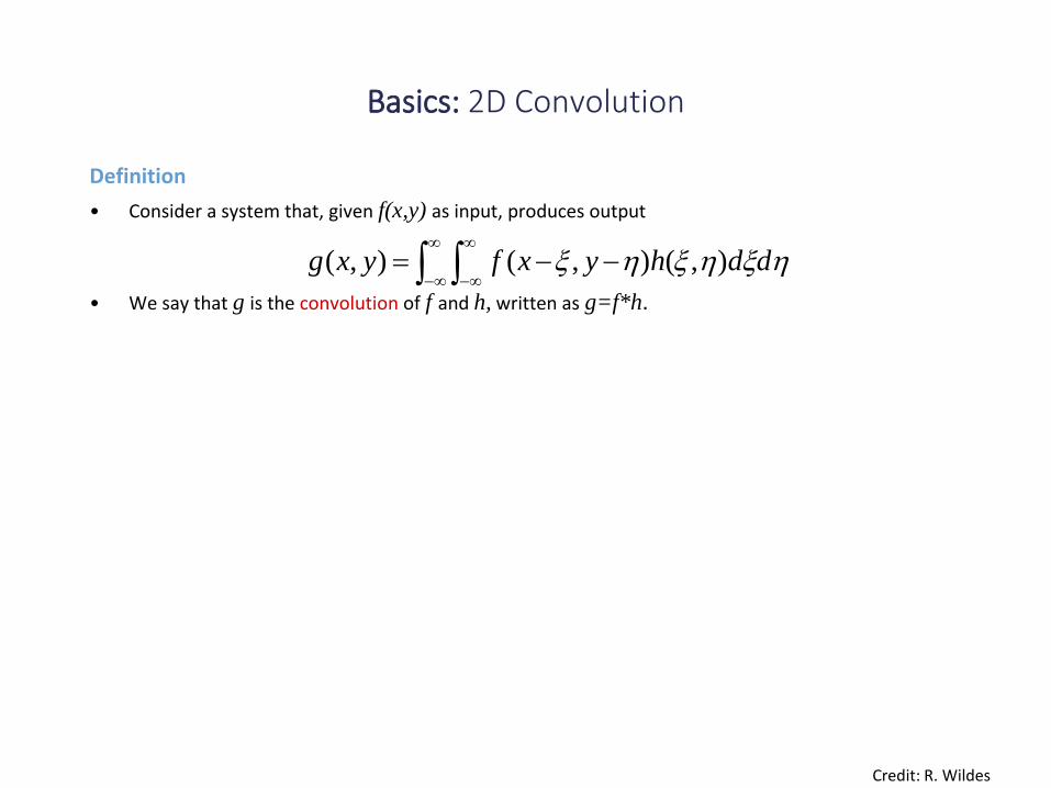
Basics: 2D Convolution
Definition
• Consider a system that, given f(x,y) as input, produces output
• We say that g is the convolution of f and h, written as g=f*h.
ddhyxfyxg ),(),(),(
Credit: R. Wildes

Basics: Another convolution example
Graphic depiction Numerical calculation
Formalization
*
x s f(x-s)h(s) +
-2 -1
0
1
-1 -1
0
1
0 -1
0
1
1 -1
0
1
2 -1
0
1
f
h
f*h
dsshsxf )()(
Credit: R. Wildes
2
1
1

Basics: Another convolution example
Graphic depiction Numerical calculation
Formalization
*
x s f(x-s)h(s) +
-2 -1 (1)(1)
0 (1)(0)
1 (1)(-1) 0
-1 -1
0
1
0 -1
0
1
1 -1
0
1
2 -1
0
1
f
h
f*h
dsshsxf )()(
Credit: R. Wildes
2
1
1h
s = -1 0 1

Basics: Another convolution example
Graphic depiction Numerical calculation
Formalization
*
x s f(x-s)h(s) +
-2 -1 (1)(1)
0 (1)(0)
1 (1)(-1) 0
-1 -1
0
1
0 -1
0
1
1 -1
0
1
2 -1
0
1
f
h
f*h
dsshsxf )()(
Credit: R. Wildes

Basics: Another convolution example
Graphic depiction Numerical calculation
Formalization
*
x s f(x-s)h(s) +
-2 -1 (1)(1)
0 (1)(0)
1 (1)(-1) 0
-1 -1 (3/2)(1)
0 (1)(0)
1 (1)(-1) 1/2
0 -1
0
1
1 -1
0
1
2 -1
0
1
f
h
f*h
dsshsxf )()(
Credit: R. Wildes
2
1
1h

Basics: Another convolution example
Graphic depiction Numerical calculation
Formalization
*
x s f(x-s)h(s) +
-2 -1 (1)(1)
0 (1)(0)
1 (1)(-1) 0
-1 -1 (3/2)(1)
0 (1)(0)
1 (1)(-1) 1/2
0 -1 (2)(1)
0 (3/2)(0)
1 (1)(-1) 1
1 -1
0
1
2 -1
0
1
f
h
f*h
dsshsxf )()(
Credit: R. Wildes
2
1
1h

Basics: Another convolution example
Graphic depiction Numerical calculation
Formalization
*
x s f(x-s)h(s) +
-2 -1 (1)(1)
0 (1)(0)
1 (1)(-1) 0
-1 -1 (3/2)(1)
0 (1)(0)
1 (1)(-1) 1/2
0 -1 (2)(1)
0 (3/2)(0)
1 (1)(-1) 1
1 -1 (2)(1)
0 (2)(0)
1 (3/2)(-1) 1/2
2 -1 (2)(1)
0 (2)(0)
1 (2)(-1) 0
f
h
f*h
dsshsxf )()(
Credit: R. Wildes
2
1
1h

Basics: Convolution
Definition
• Consider a system that, given f(x,y) as input, produces output
• We say that g is the convolution of f and h, written as g=f*h.
Convolution is linear
• Applying the system to (a f1(x,y) + b f2(x,y)) yields (a g1(x,y) + b g2(x,y)).
• Follows from rule for integrating the product of a constant and a function
• and the rule for integrating the sum of two functions.
ddhyxfyxg ),(),(),(
dbdadba )()()()(
Credit: R. Wildes
Basics: Convolution
Definition
• Consider a system that, given f(x,y) as input, produces output
• We say that g is the convolution of f and h, written as g=f*h.
Convolution is linear
• Applying the system to (a f1(x,y) + b f2(x,y)) yields (a g1(x,y) + b g2(x,y)).
• Follows from rule for integrating the product of a constant and a function
• and the rule for integrating the sum of two functions.
Convolution is shift invariant
• Applying the system to f(x-a,y-b) yields g(x-a,y-b).
• Follows from the convolution integral being independent of (x,y)
• So a change of variables (x,y)(x-a,y-b)=(x’,y’) just shifts the result.
• Another way to think of shift invariance is that the operation (e.g. *) “behaves the same everywhere”
• For images: The value of the output depends on the pattern in the image neighborhood, not the position of the neighborhood
ddhyxfyxg ),(),(),(
Credit: R. Wildes

Images as functions
• We can think of an image as a function, f, from
R2 to R:• f( x, y ) gives the intensity at position ( x, y )
• Realistically, we expect the image only to be defined over a
rectangle, with a finite range:
– f: [a,b] x [c,d] [0, 1.0]
• A color image is just three functions pasted
together. We can write this as a “vector-valued”
function: ( , )
( , ) ( , )
( , )
r x y
f x y g x y
b x y
Credit: S. Seitz

Digital images
• In computer vision we operate on digital (discrete) images:• Sample the 2D space on a regular grid
• Quantize each sample (round to nearest integer)
• Image thus represented as a matrix of integer values.
Credit: S. Seitz
2D
1D

Image filtering
• Modify the pixels in an image based on some function of a local neighborhood of each pixel
5 14
1 71
5 310
Local image data
7
Modified image data
Some function
Credit: L. Zhang

Linear filtering
• One simple version: linear filtering (cross-correlation, convolution)
– Replace each pixel by a linear combination (a weighted sum) of its neighbors
• The prescription for the linear combination is called the “kernel” (or “mask”, “filter”)
0.5
0.5 00
10
0 00
kernel
8
Modified image data
Credit: L. Zhang
Local image data
6 14
1 81
5 310
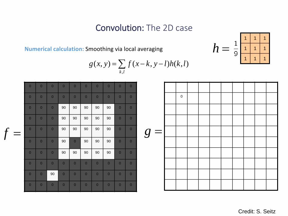
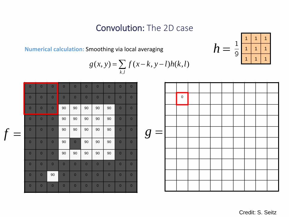
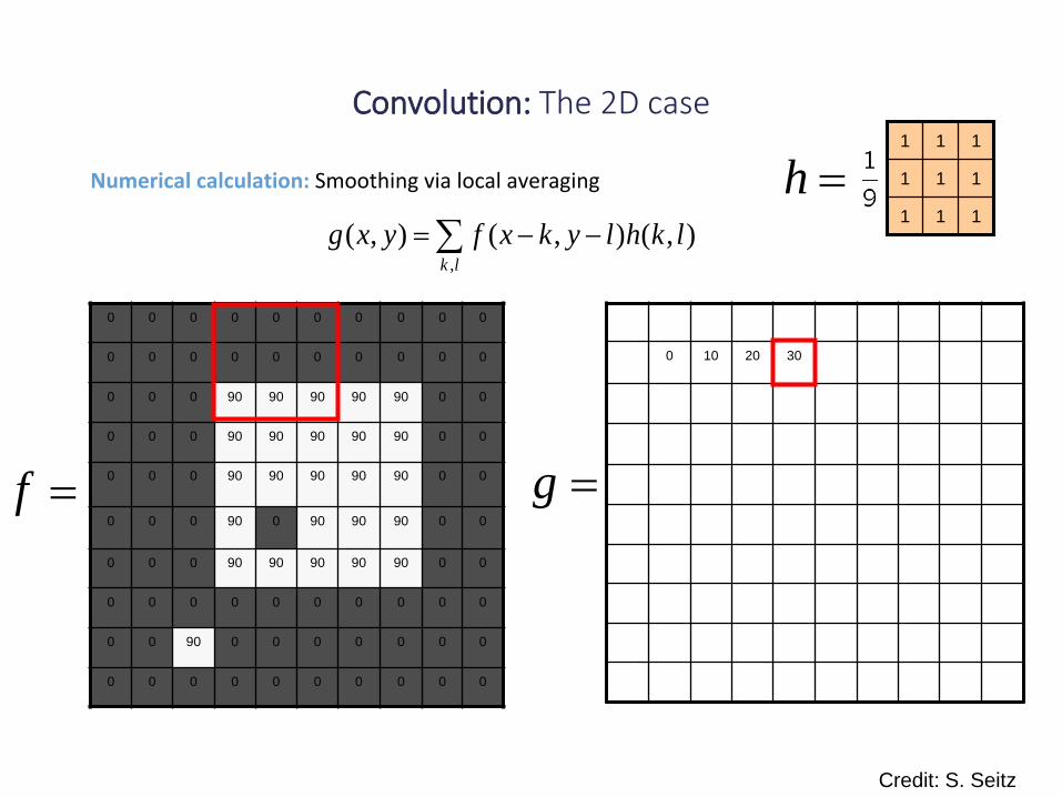
Convolution: The 2D case
Numerical calculation: Smoothing via local averaging
0
0 0 0 0 0 0 0 0 0 0
0 0 0 0 0 0 0 0 0 0
0 0 0 90 90 90 90 90 0 0
0 0 0 90 90 90 90 90 0 0
0 0 0 90 90 90 90 90 0 0
0 0 0 90 0 90 90 90 0 0
0 0 0 90 90 90 90 90 0 0
0 0 0 0 0 0 0 0 0 0
0 0 90 0 0 0 0 0 0 0
0 0 0 0 0 0 0 0 0 0
111
111
111
h
gf
Credit: S. Seitz
lk
lkhlykxfyxg,
),(),(),(
Convolution: The 2D case
Numerical calculation: Smoothing via local averaging
lk
lkhlykxfyxg,
),(),(),(
0
0 0 0 0 0 0 0 0 0 0
0 0 0 0 0 0 0 0 0 0
0 0 0 90 90 90 90 90 0 0
0 0 0 90 90 90 90 90 0 0
0 0 0 90 90 90 90 90 0 0
0 0 0 90 0 90 90 90 0 0
0 0 0 90 90 90 90 90 0 0
0 0 0 0 0 0 0 0 0 0
0 0 90 0 0 0 0 0 0 0
0 0 0 0 0 0 0 0 0 0
111
111
111
h
gf
Credit: S. Seitz

Convolution: The 2D case
Numerical calculation: Smoothing via local averaging
lk
lkhlykxfyxg,
),(),(),(
0 10
0 0 0 0 0 0 0 0 0 0
0 0 0 0 0 0 0 0 0 0
0 0 0 90 90 90 90 90 0 0
0 0 0 90 90 90 90 90 0 0
0 0 0 90 90 90 90 90 0 0
0 0 0 90 0 90 90 90 0 0
0 0 0 90 90 90 90 90 0 0
0 0 0 0 0 0 0 0 0 0
0 0 90 0 0 0 0 0 0 0
0 0 0 0 0 0 0 0 0 0
111
111
111
h
gf
Credit: S. Seitz

Convolution: The 2D case
Numerical calculation: Smoothing via local averaging
lk
lkhlykxfyxg,
),(),(),(
0 10 20
0 0 0 0 0 0 0 0 0 0
0 0 0 0 0 0 0 0 0 0
0 0 0 90 90 90 90 90 0 0
0 0 0 90 90 90 90 90 0 0
0 0 0 90 90 90 90 90 0 0
0 0 0 90 0 90 90 90 0 0
0 0 0 90 90 90 90 90 0 0
0 0 0 0 0 0 0 0 0 0
0 0 90 0 0 0 0 0 0 0
0 0 0 0 0 0 0 0 0 0
111
111
111
h
gf
Credit: S. Seitz
Convolution: The 2D case
Numerical calculation: Smoothing via local averaging
lk
lkhlykxfyxg,
),(),(),(
0 10 20 30
0 0 0 0 0 0 0 0 0 0
0 0 0 0 0 0 0 0 0 0
0 0 0 90 90 90 90 90 0 0
0 0 0 90 90 90 90 90 0 0
0 0 0 90 90 90 90 90 0 0
0 0 0 90 0 90 90 90 0 0
0 0 0 90 90 90 90 90 0 0
0 0 0 0 0 0 0 0 0 0
0 0 90 0 0 0 0 0 0 0
0 0 0 0 0 0 0 0 0 0
111
111
111
h
gf
Credit: S. Seitz

Convolution: The 2D case
Numerical calculation: Smoothing via local averaging
lk
lkhlykxfyxg,
),(),(),(
0 10 20 30 30
0 0 0 0 0 0 0 0 0 0
0 0 0 0 0 0 0 0 0 0
0 0 0 90 90 90 90 90 0 0
0 0 0 90 90 90 90 90 0 0
0 0 0 90 90 90 90 90 0 0
0 0 0 90 0 90 90 90 0 0
0 0 0 90 90 90 90 90 0 0
0 0 0 0 0 0 0 0 0 0
0 0 90 0 0 0 0 0 0 0
0 0 0 0 0 0 0 0 0 0
111
111
111
h
gf
Credit: S. Seitz

Convolution: The 2D case
Numerical calculation: Smoothing via local averaging
lk
lkhlykxfyxg,
),(),(),(
0 10 20 30 30 30
0 0 0 0 0 0 0 0 0 0
0 0 0 0 0 0 0 0 0 0
0 0 0 90 90 90 90 90 0 0
0 0 0 90 90 90 90 90 0 0
0 0 0 90 90 90 90 90 0 0
0 0 0 90 0 90 90 90 0 0
0 0 0 90 90 90 90 90 0 0
0 0 0 0 0 0 0 0 0 0
0 0 90 0 0 0 0 0 0 0
0 0 0 0 0 0 0 0 0 0
111
111
111
h
gf
?
Credit: S. Seitz

Convolution: The 2D case
Numerical calculation: Smoothing via local averaging
lk
lkhlykxfyxg,
),(),(),(
0 10 20 30 30 30
0 0 0 0 0 0 0 0 0 0
0 0 0 0 0 0 0 0 0 0
0 0 0 90 90 90 90 90 0 0
0 0 0 90 90 90 90 90 0 0
0 0 0 90 90 90 90 90 0 0
0 0 0 90 0 90 90 90 0 0
0 0 0 90 90 90 90 90 0 0
0 0 0 0 0 0 0 0 0 0
0 0 90 0 0 0 0 0 0 0
0 0 0 0 0 0 0 0 0 0
111
111
111
h
gf50
Credit: S. Seitz

Convolution: The 2D case
Numerical calculation: Smoothing via local averaging
lk
lkhlykxfyxg,
),(),(),(
0 0 0 0 0 0 0 0 0 0
0 0 0 0 0 0 0 0 0 0
0 0 0 90 90 90 90 90 0 0
0 0 0 90 90 90 90 90 0 0
0 0 0 90 90 90 90 90 0 0
0 0 0 90 0 90 90 90 0 0
0 0 0 90 90 90 90 90 0 0
0 0 0 0 0 0 0 0 0 0
0 0 90 0 0 0 0 0 0 0
0 0 0 0 0 0 0 0 0 0
111
111
111
h
gf
0 10 20 30 30 30 20 10
0 20 40 60 60 60 40 20
0 30 60 90 90 90 60 30
0 30 50 80 80 90 60 30
0 30 50 80 80 90 60 30
0 20 30 50 50 60 40 20
10 20 30 30 30 30 20 10
10 10 10 0 0 0 0 0
Credit: S. Seitz

Convolution vs. correlation
Let f be the image and g be the kernel, the cross-correlation operation is defined as
Note: We have defined convolution as g=f*h
For a symmetric kernel, how will the outputs differ?
If the input is an impulse signal, how will the outputs differ?
lk
lkhlykxfyxg,
),(),(),(
lk
lkhlykxfyxg,
),(),(),(
fFilter kernel is “flipped”in both dimensions (bottom to top, right to left)
Then cross-correlation is applied
f

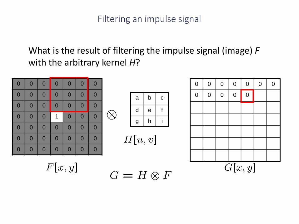
Filtering an impulse signal
0 0 0 0 0 0 0
0 0 0 0 0 0 0
0 0 0 0 0 0 0
0 0 0 1 0 0 0
0 0 0 0 0 0 0
0 0 0 0 0 0 0
0 0 0 0 0 0 0
a b c
d e f
g h i
What is the result of filtering the impulse signal (image) F with the arbitrary kernel H?
?
Credit: K. Grauman
Filtering an impulse signal
0 0 0 0 0 0 0
0 0 0 0 0 0 0
0 0 0 0 0 0 0
0 0 0 1 0 0 0
0 0 0 0 0 0 0
0 0 0 0 0 0 0
0 0 0 0 0 0 0
a b c
d e f
g h i
0 0 0 0 0 0 0
0 0 0 0 0
What is the result of filtering the impulse signal (image) F with the arbitrary kernel H?

Filtering an impulse signal
0 0 0 0 0 0 0
0 0 0 0 0 0 0
0 0 0 0 0 0 0
0 0 0 1 0 0 0
0 0 0 0 0 0 0
0 0 0 0 0 0 0
0 0 0 0 0 0 0
a b c
d e f
g h i
0 0 0 0 0 0 0
0 0 0 0 0 0 0
0 0
What is the result of filtering the impulse signal (image) F with the arbitrary kernel H?

Filtering an impulse signal
0 0 0 0 0 0 0
0 0 0 0 0 0 0
0 0 0 0 0 0 0
0 0 0 1 0 0 0
0 0 0 0 0 0 0
0 0 0 0 0 0 0
0 0 0 0 0 0 0
a b c
d e f
g h i
0 0 0 0 0 0 0
0 0 0 0 0 0 0
0 0 i
What is the result of filtering the impulse signal (image) F with the arbitrary kernel H?

Filtering an impulse signal
0 0 0 0 0 0 0
0 0 0 0 0 0 0
0 0 0 0 0 0 0
0 0 0 1 0 0 0
0 0 0 0 0 0 0
0 0 0 0 0 0 0
0 0 0 0 0 0 0
a b c
d e f
g h i
0 0 0 0 0 0 0
0 0 0 0 0 0 0
0 0 i h
What is the result of filtering the impulse signal (image) F with the arbitrary kernel H?

Filtering an impulse signal
0 0 0 0 0 0 0
0 0 0 0 0 0 0
0 0 0 0 0 0 0
0 0 0 1 0 0 0
0 0 0 0 0 0 0
0 0 0 0 0 0 0
0 0 0 0 0 0 0
a b c
d e f
g h i
0 0 0 0 0 0 0
0 0 0 0 0 0 0
0 0 i h g 0 0
0 0 f e
What is the result of filtering the impulse signal (image) F with the arbitrary kernel H?

Filtering an impulse signal
0 0 0 0 0 0 0
0 0 0 0 0 0 0
0 0 0 0 0 0 0
0 0 0 1 0 0 0
0 0 0 0 0 0 0
0 0 0 0 0 0 0
0 0 0 0 0 0 0
a b c
d e f
g h i
0 0 0 0 0 0 0
0 0 0 0 0 0 0
0 0 i h g 0 0
0 0 f e d 0 0
0 0 c b a
What is the result of filtering the impulse signal (image) F with the arbitrary kernel H?

Filtering an impulse signal
0 0 0 0 0 0 0
0 0 0 0 0 0 0
0 0 0 0 0 0 0
0 0 0 1 0 0 0
0 0 0 0 0 0 0
0 0 0 0 0 0 0
0 0 0 0 0 0 0
a b c
d e f
g h i
0 0 0 0 0 0 0
0 0 0 0 0 0 0
0 0 i h g 0 0
0 0 f e d 0 0
0 0 c b a 0 0
0 0 0 0 0 0 0
0 0 0 0 0 0 0
What is the result of filtering the impulse signal (image) F with the arbitrary kernel H?

Filtering an impulse signal
0 0 0 0 0 0 0
0 0 0 0 0 0 0
0 0 0 0 0 0 0
0 0 0 1 0 0 0
0 0 0 0 0 0 0
0 0 0 0 0 0 0
0 0 0 0 0 0 0
a b c
d e f
g h i
i h g
f e d
c b a
What is the result of filtering the impulse signal (image) F with the arbitrary kernel H?
Filter output is reversed.

Convolution
• Convolution: – Flip the filter in both dimensions (bottom to top, right to left)
– Then apply cross-correlation
Notation for convolution operator
F
H
Credit: K. Grauman

Practice with linear filters
000
010
000
Original
?
Credit: D. Lowe
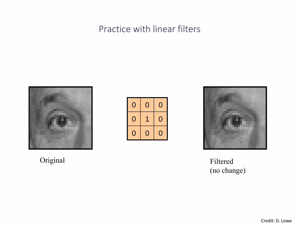
Practice with linear filters
000
010
000
Original Filtered
(no change)
Credit: D. Lowe

Practice with linear filters
000
100
000
Original
?
Credit: D. Lowe

Practice with linear filters
000
100
000
Original Shifted left
By 1 pixel
Credit: D. Lowe

Practice with linear filters
Original
111
111
111
000
020
000
- ?
(Note that filter sums to 1)
Credit: D. Lowe

Practice with linear filters
Original
111
111
111
000
020
000
-
Sharpening filter
- Accentuates differences with local
average
Credit: K. Grauman

Sharpening
original
0
2.0
0
0.33
Sharpened
original
Slide credit: Bill Freeman

Sharpening example
coef
fici
ent
-0.3original
8
Sharpened
(differences are
accentuated; constant
areas are left untouched).
11.21.7
-0.25
8
Slide credit: Bill Freeman

Sharpening
Credit: D. Lowe

Other filters
-101
-202
-101
Vertical Edge
(absolute value)
Sobel
Credit: D. Lowe
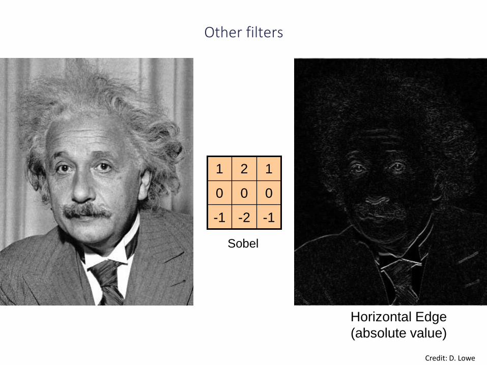
Other filters
-1-2-1
000
121
Horizontal Edge
(absolute value)
Sobel
Credit: D. Lowe

Border treatment
• What about near the edge?
– the filter window falls off the edge of the image
– need to extrapolate
– methods:
• clip filter (black)
• wrap around
• copy edge
• reflect across edge
Credit: S. Marschner

Border treatment
• What is the size of the output?
– shape = ‘full’: output size is sum of sizes of f and g
– shape = ‘same’: output size is same as f
– shape = ‘valid’: output size is difference of sizes of f and g
f
gg
gg
f
gg
gg
f
gg
gg
full same valid
Credit: S. Lazebnik

Smoothing by averaging
depicts box filter: white = high value, black = low value
original filtered
Credit: D. Forsyth

Important filter: Gaussian
0 0 0 0 0 0 0 0 0 0
0 0 0 0 0 0 0 0 0 0
0 0 0 90 90 90 90 90 0 0
0 0 0 90 90 90 90 90 0 0
0 0 0 90 90 90 90 90 0 0
0 0 0 90 0 90 90 90 0 0
0 0 0 90 90 90 90 90 0 0
0 0 0 0 0 0 0 0 0 0
0 0 90 0 0 0 0 0 0 0
0 0 0 0 0 0 0 0 0 0
1 2 1
2 4 2
1 2 1
• What if we want nearest neighboring pixels to have the most influence on the output?
This kernel is an approximation of a Gaussian function:
Credit: S. Seitz

• Weight contributions of neighboring pixels by nearness
0.003 0.013 0.022 0.013 0.0030.013 0.059 0.097 0.059 0.0130.022 0.097 0.159 0.097 0.0220.013 0.059 0.097 0.059 0.0130.003 0.013 0.022 0.013 0.003
5 x 5, = 1
Important filter: Gaussian
Credit: C. Rasmussen

Important filter: Gaussian
• Gaussian filters have some interesting properties
• Common in many natural models
• Smooth and symmetric function it has an infinite number of derivatives
• Fourier Transform of Gaussian is Gaussian (see later)
• Convolution of a Gaussian with itself is a Gaussian
• Gaussian is separable (e.g. 2D convolution can be performed by two 1-D convolutions)
• There is evidence that the human visual system performs Gaussian filtering
0.003 0.013 0.022 0.013 0.0030.013 0.059 0.097 0.059 0.0130.022 0.097 0.159 0.097 0.0220.013 0.059 0.097 0.059 0.0130.003 0.013 0.022 0.013 0.003
5 x 5, = 1

Smoothing with a Gaussian
Credit: D. Forsyth
•Remove “high-frequency” components from the image (low-pass filter)Images become more smooth

Gaussian filters
• What parameters matter here?
• Size of kernel or mask
– Note, Gaussian function has infinite support, but discrete filters use finite kernels
σ = 5 with 10 x 10 kernel
σ = 5 with 30 x 30 kernel
Credit: K. Grauman

Gaussian filters
• What parameters matter here?
• Variance of Gaussian: determines extent of smoothing
• Rule of thumb: filter width of about 6σ
σ = 2 with 30 x 30 kernel
σ = 5 with 30 x 30 kernel
Credit: K. Grauman

Basics: More facts about convolution
Convolution is commutative
• That is f*h = h*f
• Interchange of h and f possible
• Order does not care
Convolution is associative
• That is (f*h1)*h2 = f*(h1*h2)
• Can be exploited for efficient implementations
f gh
gh f
f h1 h2 g
f h1*h2 g
Credit: R. Wildes

Gaussian filters
Note: Convolution is associative: (f*g)*h = f*(g*h)
• Can be exploited for multi-scale processing and efficiency:
– Convolving two times with Gaussian kernel of width σ is same as convolving once with kernel of width σ√2
– Efficiency: multiple smoothing with small-width kernel delivers same result as larger-width kernel
Credit: I. Kokkinos
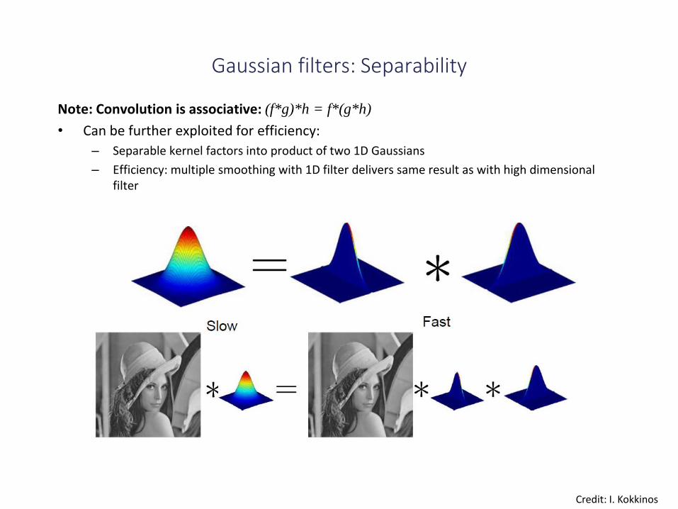
Gaussian filters: Separability
Note: Convolution is associative: (f*g)*h = f*(g*h)
• Can be further exploited for efficiency:
– Separable kernel factors into product of two 1D Gaussians
– Efficiency: multiple smoothing with 1D filter delivers same result as with high dimensional filter
Credit: I. Kokkinos

Separability of the Gaussian filter for 2D
Credit: D. Lowe

Separability: Numeric example for 2D
• 2D filters are separable if they can be expressed as the outer product of two vectors. For example:
Note: Convolution is associative: (f*g)*h = f*(g*h)
g
h
f
Credit: K. Grauman
For MN image, PQ filter: 2D takes MNPQ add/times,
while 1D takes MN(P + Q)
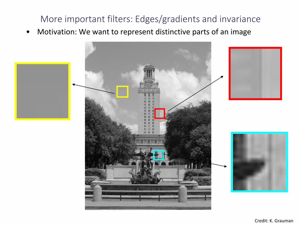
More important filters: Edges/gradients and invariance
Credit: K. Grauman
• Motivation: We want to represent distinctive parts of an image

Derivatives and edges
imageintensity function
(along horizontal scanline) first derivative
edges correspond to
extrema of derivative
An edge is a place of rapid change in the
image intensity function.
Credit: L. Lazebnik

More important filters: Derivative of Gaussian
11 0.0030 0.0133 0.0219 0.0133 0.00300.0133 0.0596 0.0983 0.0596 0.01330.0219 0.0983 0.1621 0.0983 0.02190.0133 0.0596 0.0983 0.0596 0.01330.0030 0.0133 0.0219 0.0133 0.0030
)()( hgIhgI
Credit: K. Grauman

More important filters: Derivative of Gaussian
x-direction y-direction
Credit: L. Lazebnik

Gaussian filters: Steerability
Credit: I. Kokkinos
Steerable filter:

More important filters: Derivative(s) of Gaussian
• is the Laplacian operator:
Laplacian of Gaussian
Gaussian derivative of Gaussian
Credit: K. Grauman

The Fourier transform
Further reading: Szeliski, Richard. Computer Vision: Algorithms and Applications. Springer, 2010, Chapter 3, Section 3.4

Linear image transformations
• In analyzing images, it’s often useful to make a change of basis.
Fourier transform, or
Wavelet transform, or
Steerable pyramid transform
fUF
Vectorized image
transformed image
Credit: B. Freeman
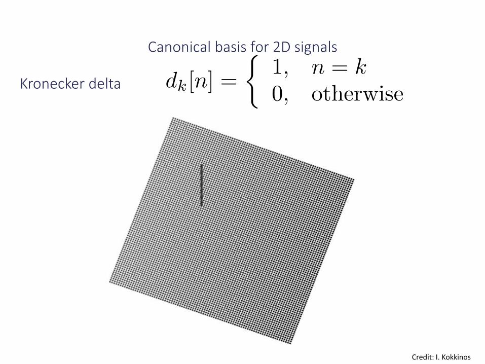
Canonical basis for 2D signals
Kronecker delta
Credit: I. Kokkinos

Fourier Transform = Change of Basis
Credit: I. Kokkinos
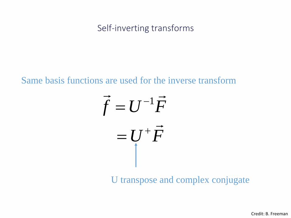
Self-inverting transforms
FU
FUf
1
Same basis functions are used for the inverse transform
U transpose and complex conjugate
Credit: B. Freeman

Jean Baptiste Joseph Fourier (1768-1830)
had crazy idea (1807):Any univariate function can be rewritten as a weighted sum of sines and cosines of different frequencies.
• Don’t believe it?
– Neither did Lagrange, Laplace, Poisson and others
– Not translated into English until 1878!
• But it’s true!
– called Fourier Series
...the manner in which the author arrives at these equations is not exempt of difficulties and...his
analysis to integrate them still leaves something to be desired on the score of generality and even rigour.
Laplace
LagrangeLegendre
Credit: J. Hays

Fourier Transform
Our building block:
Add enough of them to get any signal g(x) you want!
The Fourier transform F(w)stores the magnitude and phase at each frequency
Magnitude encodes how much signal there is at a particular frequency
Phase encodes spatial information (indirectly)
fwxAsin(
Credit: J. Hays
f
A
w

Fourier Transform
•We want to understand the frequency w of our signal. So, let’s reparametrize the signal by w instead of x:
fwxAsin(
f(x) F(w)Fourier
Transform
F(w) f(x)Inverse Fourier
Transform
For every w from 0 to inf, F(w) holds the amplitude A
and phase f of the corresponding sine • How can F hold both? Complex number trick!
)()()( www iIRF 22 )()( ww IRA
)(
)(tan 1
w
wf
R
I
We can always go back:
Credit: A. Efros

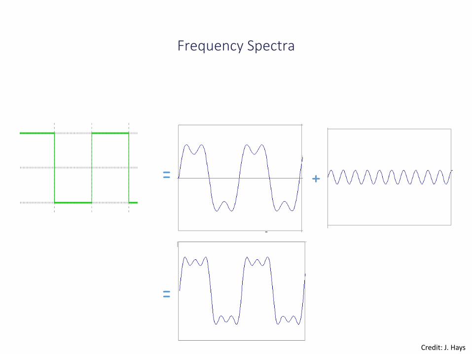
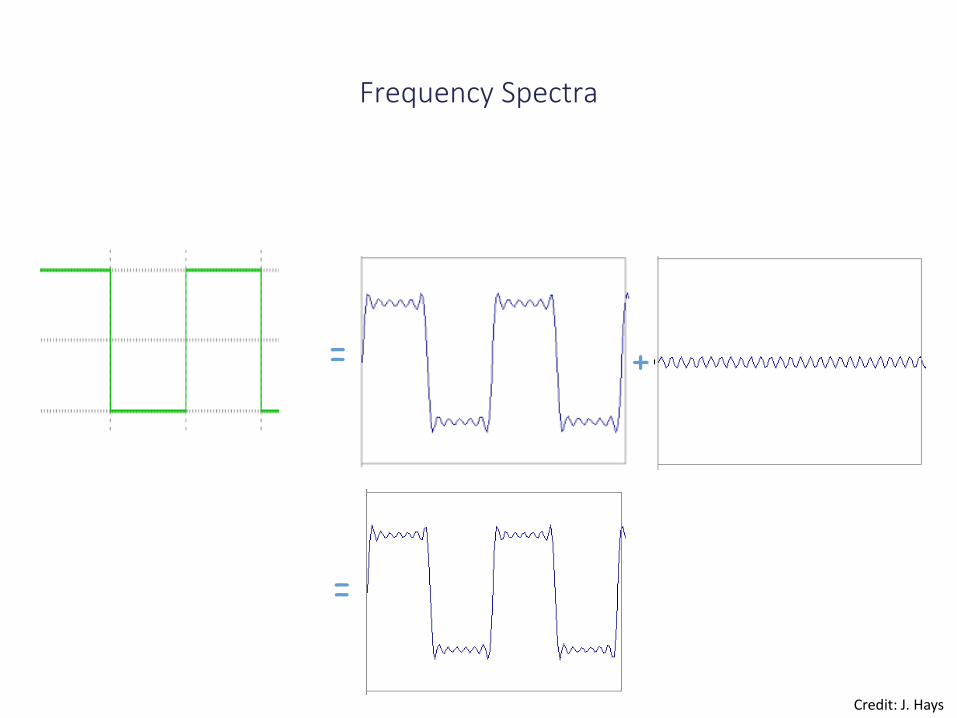
Frequency Spectra
• example : g(t) = sin(2πf t) + (1/3)sin(2π(3f) t)
= +
Credit: A. Efros

Frequency Spectra
Credit: J. Hays

= +
=
Frequency Spectra
Credit: J. Hays
= +
=
Frequency Spectra
Credit: J. Hays

= +
=
Frequency Spectra
Credit: J. Hays

= +
=
Frequency Spectra
Credit: J. Hays
= +
=
Frequency Spectra
Credit: J. Hays

= 1
1sin(2 )
k
A ktk
Frequency Spectra
Credit: J. Hays

Basics: The Fourier transform
Eigenfunctions
• An eigenfunction of a system is one that is simply multiplied by another factor in the output.
• We think of this as analogous to the case of eigenvectors from linear algebra.
f(w) A(w) f(w)
Credit: R. Wildes

Basics: The Fourier transform
Eigenfunctions
• An eigenfunction of a system is one that is simply multiplied by another factor in the output.
• We think of this as analogous to the case of eigenvectors from linear algebra.
Remark
• Notation
with the imaginary number
f(w) A(w) f(w)
)exp(iwteiwt
1i
Credit: R. Wildes

Basics: The Fourier transform
Eigenfunctions
• An eigenfunction of a system is one that is simply multiplied by another factor in the output.
• We think of this as analogous to the case of eigenvectors from linear algebra.
• For the case of 1D Linear Shift Invariant (LSI) systems we find that exp(iwt) is an eigenfunction of convolution.
• Here A(w) is the (possibly complex) factor by which the input signal is multiplied.
• So, from the input exponential we obtain another exponential; but, scaled and shifted in phase.
f(w) A(w) f(w)
exp(iwt) A(w) exp(iwt)
Credit: R. Wildes

Basics: The Fourier transform
Eigenfunctions
• An eigenfunction of a system is one that is simply multiplied by another factor in the output.
• We think of this as analogous to the case of eigenvectors from linear algebra.
• For the case of 1D LSI systems we find that exp(iwt) is an eigenfunction of convolution.
• Here A(w) is the (possibly complex) factor by which the input signal is multiplied.
• So, from the input exponential we obtain another exponential; but, scaled and shifted in phase.
Frequency
• We call w the frequency (or wave number) of the eigenfunction.
• In practice, we use real waveforms, like cos(wt) and sin(wt), with the relationship
exp(iwt)=cos(wt) + i sin(wt)
which is known as Euler’s relation.
• The complex exponential is used in derivations simply because it provides a compact notation.
f(w) A(w) f(w)
exp(iwt) A(w) exp(iwt)
Credit: R. Wildes

Basics: The Fourier transform
1D frequency• We consider functions of the form
f(x) = Acos(ux + d)
where
A is the amplitude
u is the (angular) frequency
d is the phase constant.
• Notice that the function repeats its value when ux + d increases by .
• For example, when d = 0, the maxima and minima occur when , for k an integer.kux
x
f(x)
A
d/u
u/2
2
Credit: R. Wildes

115
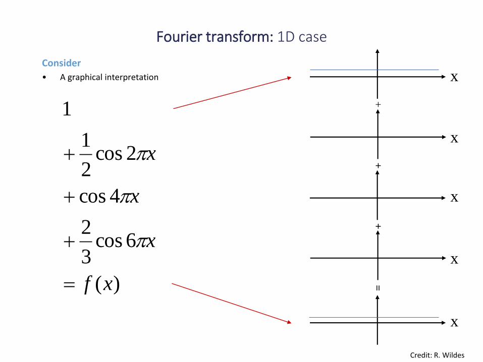
Fourier transform: 1D case
Consider
• A graphical interpretation
)(
6cos3
2
4cos
2cos2
1
1
xf
x
x
x
+
+
+
=
x
x
x
x
x
Credit: R. Wildes
Consider
• A graphical interpretation
)(
6cos3
2
4cos
2cos2
1
1
xf
x
x
x
+
+
+
=
x
x
x
x
x
Fourier transform: 1D case
Credit: R. Wildes

Fourier transform: 1D case
Consider
• A graphical interpretation
)(
6cos3
2
4cos
2cos2
1
1
xf
x
x
x
+
+
+
=
x
x
x
x
x
Credit: R. Wildes

Fourier transform: 1D case
Consider
• A graphical interpretation
)(
6cos3
2
4cos
2cos2
1
1
xf
x
x
x
+
+
+
x
x
x
x
x
=
=
Credit: R. Wildes

Fourier transform: 1D case
Consider• A graphical interpretation
Observation• Complicated signals can be represented as
the sum of simple components.
)(
6cos3
2
4cos
2cos2
1
1
xf
x
x
x
+
+
+
x
x
x
x
x
=
Credit: R. Wildes

Fourier transform: 1D case
+
+
+
x
x
x
x
x
=
u
u
u
u
u
f(x)
+
+
+
=
6;cos3
26cos
3
2
4;cos14cos
2;cos2
12cos
2
1
0;cos10cos1
uuxx
uuxx
uuxx
uuxx
Credit: R. Wildes

Fourier transform: 1D case
+
+
+
x
x
x
x
x
=
u
u
u
u
u
f(x)
+
+
+
=
6;cos3
26cos
3
2
4;cos14cos
2;cos2
12cos
2
1
0;cos10cos1
uuxx
uuxx
uuxx
uuxx
Note• By symmetry, we may choose
to represent this as uCredit: R. Wildes

The Fourier transform of an image
Source image (J. Fourier) Fourier power spectrum
Credit: R. Wildes

Basics: The 2D Fourier transform
2D Eigenfunctions
• For the case of 1D LSI systems we found that exp(iwt) is an eigenfunction of convolution.
• One can show that that exp[i(ux+vy)] is an eigenfunction in 2D.
• The 2D Fourier transform F(u,v) of f(x,y) is given by
exp[i(ux+vy)] A(u,v) exp[i(ux+vy)]
Credit: R. Wildes
exp(iwt) A(w) exp(iwt)
dxdyvyuxiyxfvuF )](exp[),(),(
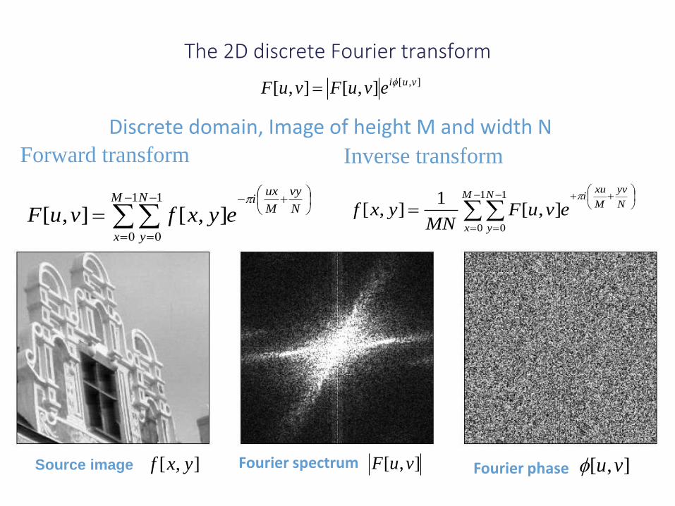
The 2D discrete Fourier transform
Discrete domain, Image of height M and width N
1
0
1
0
],[1
],[M
x
N
y
N
yv
M
xui
evuFMN
yxf
Inverse transform
1
0
1
0
],[],[M
x
N
y
N
vy
M
uxi
eyxfvuF
Forward transform
Source image ],[ vuFFourier spectrum],[ yxf ],[ vufFourier phase
],[],[],[ vuievuFvuF f

Basics: The Fourier transform
2D frequency
• For two spatial dimensions, we see that there are two corresponding frequency
components, u and v.
• We refer to the uv-plane as the frequency domain.
• We refer to the xy-plane as the spatial domain.
• The real waveforms cos(ux+vy) and
sin(ux+vy) correspond to waves in 2D.
y
x
The maxima and minima
of the cosinusoids lie
along parallel equidistant
lines for k
an integer.
kvyux
(u,v)=(a,0)
Credit: R. Wildes
Cross sections orthogonal to
the ridges show a sinusoidal
profile
],[ yxf
y

Basics: The Fourier transform
2D frequency
• For two spatial dimensions, we see that there are two corresponding frequency
components, u and v.
• We refer to the uv-plane as the frequency domain.
• We refer to the xy-plane as the spatial domain.
• The real waveforms cos(ux+vy) and
sin(ux+vy) correspond to waves in 2D.
y
Cross sections orthogonal to
the ridges show a sinusoidal
profile
x
The maxima and minima
of the cosinusoids lie
along parallel equidistant
lines for k
an integer.
kvyux
(u,v)=(0,a)
Credit: R. Wildes
],[ yxf
y

Basics: The Fourier transform
2D frequency
• For two spatial dimensions, we see that there are two corresponding frequency
components, u and v.
• We refer to the uv-plane as the frequency domain.
• We refer to the xy-plane as the spatial domain.
• The real waveforms cos(ux+vy) and
sin(ux+vy) correspond to waves in 2D.
y
x
The maxima and minima
of the cosinusoids lie
along parallel equidistant
lines for k
an integer.
kvyux
Credit: R. Wildes
Cross sections orthogonal to
the ridges show a sinusoidal
profile
(u,v)/|(u,v)|
],[ yxf

The Fourier transform: 2D case
A 2D example
• Recall the 1D example
x
f(x) F(u)
u
for the cosine component
Credit: R. Wildes

The Fourier transform: 2D case
A 2D example
• Recall the 1D example
• And the interpretation of 2D spatial frequency
x
y
The maxima and minima
of the cosinusoids lie
along parallel equidistant
lines for k
an integer.
kvyux
x
f(x) F(u)F(u)
u
for the cosine component
Credit: R. Wildes
(u,v)/|(u,v)|
],[ yxf

The Fourier transform: 2D case
A 2D example
• Recall the 1D example
• Then a 2D analogue could be
x
y
x
f(x) F(u)F(u)
u
for the cosine component
Credit: R. Wildes
],[ yxf
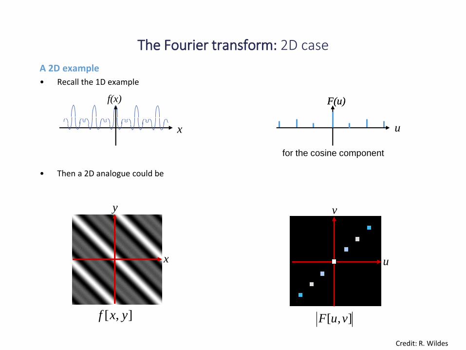
The Fourier transform: 2D case
A 2D example
• Recall the 1D example
• Then a 2D analogue could be
x
y
x
f(x) F(u)
v
u
F(u)
u
for the cosine component
Credit: R. Wildes
],[ vuF],[ yxf

To get some sense of what
basis elements look like, we
plot a basis element --- or
rather, its real part ---
as a function of x,y for some
fixed u, v. We get a function
that is constant when (ux+vy)
is constant. The magnitude of
the vector (u, v) gives a
frequency, and its direction
gives an orientation. The
function is a sinusoid with
this frequency along the
direction, and constant
perpendicular to the
direction.
u
v
vyuxie
vyuxie
Credit: B. Freeman

Here u and v
are larger than
in the previous
slide.
u
v vyuxie
vyuxie
Credit: B. Freeman

And larger still...
u
v
vyuxie
vyuxie
Credit: B. Freeman

The Fourier transform: Filtering
Intensity Image
Fourier Image
http://sharp.bu.edu/~slehar/fourier/fourier.html#filtering

The Fourier transform: Filtering
+ =
http://sharp.bu.edu/~slehar/fourier/fourier.html#filtering
More: http://www.cs.unm.edu/~brayer/vision/fourier.html

Understanding the Fourier transform of an image
Source image (J. Fourier) Fourier power spectrum
Credit: K. Derpanis

Phase and Magnitude
• Fourier transform of a real function is complex– difficult to plot, visualize
– instead, we can think of the phase and magnitude of the transform
• Phase is the phase of the complex transform
• Magnitude is the magnitude of the complex transform
• Curious fact– all natural images have about
the same magnitude transform
– hence, phase seems to matter, but magnitude largely doesn’t
• Demonstration– Take two pictures, swap the
phase transforms, compute the inverse - what does the result look like?
Credit: B. Freeman

Credit: B. Freeman

This is the
magnitude
transform
of the
cheetah pic
Credit: B. Freeman
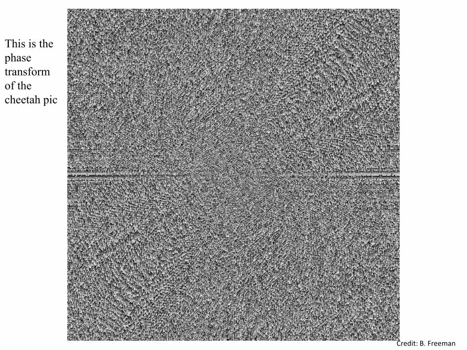
This is the
phase
transform
of the
cheetah pic
Credit: B. Freeman

Credit: B. Freeman

This is the
magnitude
transform
of the zebra
pic
Credit: B. Freeman
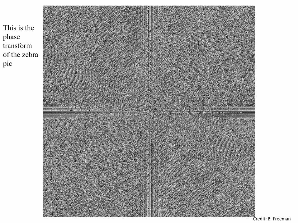
This is the
phase
transform
of the zebra
pic
Credit: B. Freeman

Reconstruction
with zebra
phase, cheetah
magnitude
Credit: B. Freeman

Reconstruction
with cheetah
phase, zebra
magnitude
Credit: B. Freeman

Extension to 3D
Credit: K. Derpanis
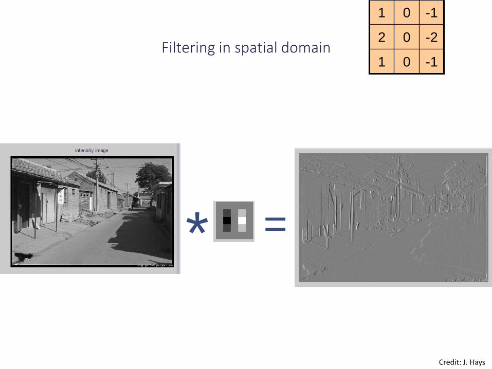
Filtering in spatial domain-101
-202
-101
* =
Credit: J. Hays

The Convolution Theorem
• The Fourier transform of the convolution of two functions is the product of their Fourier transforms
• Convolution in spatial domain is equivalent to multiplication in frequency domain!
]F[]F[]F[ hghg
]]F[][F[F* 1 hghg
Credit: J. Hays
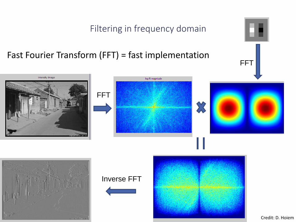
Filtering in frequency domain
FFT
FFT
Inverse FFT
=
Credit: D. Hoiem
Fast Fourier Transform (FFT) = fast implementation

Gaussian
Credit: D. Hoiem
Why does the Gaussian give a nice smooth image, but the square filter give edgy artifacts?

Box Filter
Credit: D. Hoiem
Why does the Gaussian give a nice smooth image, but the square filter give edgy artifacts?

Low pass filteringhttp://www.reindeergraphics.com
Credit: R. Fergus

High pass filteringhttp://www.reindeergraphics.com
Credit: R. Fergus

Low-pass, Band-pass, High-pass filters
low-pass:
High-pass / band-pass:
Credit: A. Efros

Why is the Frequency domain useful for us?
• The linear convolution operation can be understood from a different angle
• It can be performed very efficient using a clever implementation (FFT)
• The Frequency domain provides an alternative way to understand and manipulate the content of images

Match the spatial domain image to the Fouriermagnitude image
Credit: K. Derpanis

Spatial Domain
Basis functions:
……
……
..
Tells you where things are….
… but no concept of what it is
Credit: R. Fergus

Fourier domain
Basis functions:
Tells you what is in the image….
… but not where it is
……
……
……
Credit: R. Fergus

Modulation property and Gabor filters
Credit: I. Kokkinos

Modulation property and Gabor filters
Credit: I. Kokkinos

2D Gabor filterbank and texture analysis
Credit: I. Kokkinos

2D Gabor filterbank and texture analysis
Credit: I. Kokkinos
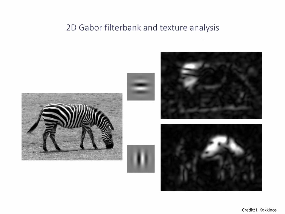
2D Gabor filterbank and texture analysis
Credit: I. Kokkinos

Summary: Images as a composition of local partsFiltering example
• Why filtering?
– Statistics of images look similar atdifferent locations
– Dependencies are very local
– Filtering is an opteration with translation equivariance
Input Feature Map
.
.
.
Credit: R. Fergus

Image Pixels Apply
Gabor filters
Spatial pool
(Sum)
Normalize to unit length
Feature Vector
Credit: R. Fergus
Summary: Compare: SIFT Descriptor

Summary
• Linear filtering and the importance of convolution
– Apply a filtermask to the local neighborhood at each pixel in the image
– The filtermask defines how to combine values from neighbors.
– Can be used for
• Extract intermediate representations to abstract images by higher-level “features”, for further processing (i.e., preserve the useful information only and discard redundancy)
• Image modification, e.g., to reduce noise, resize, increase contrast, etc.
• Match template images (e.g. by correlating two image patches)
• Image filtering in the frequency domain
– Provides a nice way to illustrate the effect of linear filtering
• Filtering is a way to modify the frequencies of images
– Efficient signal filtering is possible in that domain
– The frequency domain offers an alternative way to understanding and manipulating the image.