image-based synthesis for deep 3d human pose estimation
TRANSCRIPT

HAL Id: hal-01717188https://hal.inria.fr/hal-01717188
Submitted on 26 Feb 2018
HAL is a multi-disciplinary open accessarchive for the deposit and dissemination of sci-entific research documents, whether they are pub-lished or not. The documents may come fromteaching and research institutions in France orabroad, or from public or private research centers.
L’archive ouverte pluridisciplinaire HAL, estdestinée au dépôt et à la diffusion de documentsscientifiques de niveau recherche, publiés ou non,émanant des établissements d’enseignement et derecherche français ou étrangers, des laboratoirespublics ou privés.
Image-based Synthesis for Deep 3D Human PoseEstimation
Gregory Rogez, Cordelia Schmid
To cite this version:Gregory Rogez, Cordelia Schmid. Image-based Synthesis for Deep 3D Human Pose Estimation. Inter-national Journal of Computer Vision, Springer Verlag, 2018, 126 (9), pp.993-1008. �10.1007/s11263-018-1071-9�. �hal-01717188�

Noname manuscript No.(will be inserted by the editor)
Image-based Synthesis for Deep 3D Human Pose Estimation
Grégory Rogez · Cordelia Schmid
Received: date / Accepted: date
Abstract This paper addresses the problem of 3D humanpose estimation in the wild. A significant challenge is thelack of training data, i.e., 2D images of humans annotatedwith 3D poses. Such data is necessary to train state-of-the-artCNN architectures. Here, we propose a solution to generatea large set of photorealistic synthetic images of humans with3D pose annotations. We introduce an image-based synthesisengine that artificially augments a dataset of real images with2D human pose annotations using 3D motion capture data.Given a candidate 3D pose, our algorithm selects for eachjoint an image whose 2D pose locally matches the projected3D pose. The selected images are then combined to generatea new synthetic image by stitching local image patches ina kinematically constrained manner. The resulting imagesare used to train an end-to-end CNN for full-body 3D poseestimation. We cluster the training data into a large numberof pose classes and tackle pose estimation as a K-way classi-fication problem. Such an approach is viable only with largetraining sets such as ours. Our method outperforms mostof the published works in terms of 3D pose estimation incontrolled environments (Human3.6M) and shows promis-ing results for real-world images (LSP). This demonstratesthat CNNs trained on artificial images generalize well to realimages. Compared to data generated from more classicalrendering engines, our synthetic images do not require anydomain adaptation or fine-tuning stage.
1 Introduction
Convolutional Neural Networks (CNN) have been very suc-cessful for many different tasks in computer vision. However,
Univ. Grenoble Alpes, Inria, CNRS, Grenoble INP*, LJK,38000 Grenoble, France* Institute of Engineering Univ. Grenoble AlpesE-mail: [email protected]
training these deep architectures requires large scale datasetswhich are not always available or easily collectable. Thisis particularly the case for 3D human pose estimation, forwhich an accurate annotation of 3D articulated poses in largecollections of real images is non-trivial: annotating 2D im-ages with 3D pose information is impractical [6] while largescale 3D pose capture is only available in constrained envi-ronments through marker-based (e.g., HumanEva [49], Hu-man3.6M [20]) or makerless multiview systems (e.g., CMUPanoptic Dataset [25], MARCOnI Dataset [13]). The imagescaptured in such conditions are limited in terms of subjectsand environment diversity and do not match well real envi-ronments, i.e., real-world scenes with cluttered backgrounds.Moreover, with marker-based systems, the subjects have towear capture suits with markers on them to which learningalgorithms may overfit. This has limited the development ofend-to-end CNN architectures for real-world 3D pose under-standing.
Learning architectures usually augment existing train-ing data by applying synthetic perturbations to the originalimages, e.g., jittering exemplars or applying more complexaffine or perspective transformations [22]. Such data aug-mentation has proven to be a crucial stage, especially fortraining deep architectures. Recent work [21,37,54,64] hasintroduced the use of data synthesis as a solution to trainCNNs when only limited data is available. Synthesis can po-tentially provide infinite training data by rendering 3D CADmodels from any camera viewpoint [37,54,64]. Fisher etal. [11] generate a synthetic “Flying Chairs” dataset to learnoptical flow with a CNN and show that networks trainedon this unrealistic data still generalize very well to existingdatasets. In the context of scene text recognition, Jaderberget al. [21] trained solely on data produced by a synthetic textgeneration engine. In this case, the synthetic data is highlyrealistic and sufficient to replace real data. Although synthe-sis seems like an appealing solution, there often exists a large

2 Grégory Rogez, Cordelia Schmid
Fig. 1 Image-based synthesis engine. Input: real images with manual annotation of 2D poses, and 3D poses captured with a motion capture system.Output: 220x220 synthetic images and associated 3D poses.
domain shift from synthetic to real data [37]. Integrating ahuman 3D model in a given background in a realistic way isnot trivial [20]. Rendering a collection of photo-realistic im-ages (in terms of color, texture, context, shadow) that wouldcover the variations in pose, body shape, clothing and scenesis a challenging task.
Instead of rendering a human 3D model, we propose animage-based synthesis approach that makes use of motioncapture data to augment an existing dataset of real imageswith 2D pose annotations. Our system synthesizes a verylarge number of new images showing more pose configu-rations and, importantly, it provides the corresponding 3Dpose annotations (see Figure 1). For each candidate 3D posein the motion capture library, our system combines severalannotated images to generate a synthetic image of a humanin this particular pose. This is achieved by “copy-pasting”the image information corresponding to each joint in a kine-matically constrained manner. Given this large “in-the-wild”dataset, we implement an end-to-end CNN architecture for3D pose estimation. Our approach first clusters the 3D posesintoK pose classes. Then, aK-way CNN classifier is trainedto return a distribution over probable pose classes given abounding box around the human in the image. Our methodoutperforms most state-of-the-art results in terms of 3D poseestimation in controlled environments and shows promisingresults on images captured “in-the-wild”. The work presentedin this paper is an extension of [42]. We provide an additionalcomparison of our image-based synthesis engine with a moreclassical approach based on rendering a human 3D model.The better performance of our method shows that for traininga deep pipeline with a classification or a regression objective,it is more important to produce locally photorealistic datathan globally coherent data.
1.1 Related work
3D human pose estimation in monocular images. Recentapproaches employ CNNs for 3D pose estimation in monoc-ular images [8,28,36] or in videos [71]. Due to the lack oflarge scale training data, they are usually trained (and tested)on 3D motion capture data in constrained environments [28].Pose understanding in natural images is usually limited to 2Dpose estimation [9,59,60]. Motivated by these well-workingoff-the-shelf 2D detectors and inspired by earlier work insingle view 3D pose reconstruction [33,40,50,55], recentwork also tackles 3D pose understanding from 2D poses [2,7,15,32,58]. Some approaches use as input the 2D jointsautomatically provided by a 2D pose detector [7,32,52,62],while others jointly solve the 2D and 3D pose estimation [51,58,68]. Most similar to ours are the architectures that takeadvantage of the different sources of training data, i.e., in-door images with motion capture 3D poses and real-worldimages with 2D annotations [31,67,69]. Iqbal et al. [67] usea dual-source approach that combines 2D pose estimationwith 3D pose retrieval. Mehta et al. [31] propose a 2D-to-3Dknowledge transfer to generalize to in-the-wild images, us-ing pre-trained 2D pose networks to initialize the 3D poseregression networks. The architecture of [69] shares the com-mon representations between the 2D and the 3D tasks. Ourmethod uses the same two training sources, i.e., images withannotated 2D pose and 3D motion capture data. However, wecombine both sources off-line to generate a large training setthat is used to train an end-to-end CNN 3D pose classifier.This is shown to improve over [67], which can be explainedby the fact that training is performed in an end-to-end fashion.Synthetic pose data. A number of works have consideredthe use of synthetic data for human pose estimation. Syn-thetic data have been used for upper body [47], full-bodysilhouettes [1], hand-object interactions [45], full-body pose
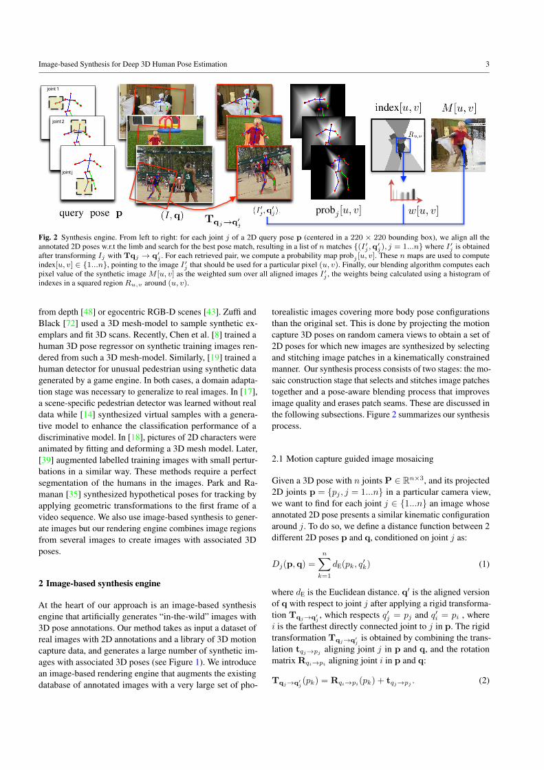
Image-based Synthesis for Deep 3D Human Pose Estimation 3
1
joint 1
joint j
joint 2
4 Grégory Rogez, Cordelia Schmid
i is the farthest directly connected joint to j in p. The rigidtransformation Tqj!q0
jis obtained by combining the trans-
lation tqj!pjaligning joint j in p and q, and the rotation
matrix Rqi!pialigning joint i in p and q:
Tqj!q0j(pk) = Rqi!pi(pk) + tqj!pj . (2)
An example of such transformation is given in Fig. 3.The function Dj measures the similarity between 2 joints
by aligning and taking into account the entire poses. To in-crease the influence of neighboring joints, we weight the dis-tances dE between each pair of joints {(pk, q0k), k = 1...n}according to their distance to the query joint j in both poses.Eq. 1 becomes:
Dj(p,q) =nX
k=1
(wjk(p) + wj
k(q)) dE(pk, q0k) (3)
where weight wjk is inversely proportional to the distance be-
tween joint k and the query joint j, i.e., wjk(p) = 1/dE(pk, pj)
and normalized so thatP
k wjk(p) = 1. This cost function is
illustrated in Fig. 3.
Fig. 3 Illustration of the cost function employed to find pose matches.We show two poses aligned at joint j with red lines across all the otherjoints denoting contributors to the distance.
For each joint j of the query pose p, we retrieve fromour dataset Q = {(I1,q1) . . . (IN ,qN )} of images and an-notated 2D poses:
qj = argminq2QDj(p,q) 8j 2 {1...n}. (4)
In practice, we do not search for self-occluded joints, i.e.,joints occluded by another body part, that can be labelled assuch by simple 3D reasoning. We obtain a list of n matches{(I 0j ,q
0j), j = 1...n} where I 0j is the cropped image obtained
after transforming Ij with Tqj!q0j. Note that a same pair
(I,q) can appear multiple times in the list of candidates, i.e.,being a good match for several joints.
Finally, to render a new image, we need to select thecandidate images I 0j to be used for each pixel (u, v). In-stead of using regular patches, we compute a probabilitymap pj [u, v] associated with each pair (I 0j ,q
0j) based on lo-
cal matches measured by dE(pk, q0k) in Eq. 1. To do so, wefirst apply a Delaunay triangulation to the set of 2D joints
in {q0j} obtaining a partition of the image into triangles, ac-
cording to the selected pose. Then, we assign the probabilityprobj(q
0k) = exp(�dE(pk, q0k)2/�2) to each vertex q0k. We
finally compute a probability map probj [u, v] by interpolat-ing values from these vertices using barycentric interpolationinside each triangle. The resulting n probability maps areconcatenated and an index map index[u, v] 2 {1...n} can becomputed as follows:
index[u, v] = argmaxj2{1...n} probj [u, v], (5)
this map pointing to the training image I 0j that should be usedfor each pixel (u, v). A mosaic M [u, v] can be generated by“copy-pasting” image information at pixel (u, v) indicated byindex[u, v]:
M [u, v] = I 0j⇤ [u, v] with j⇤ = index[u, v]. (6)
2.2 Pose-aware image blending
The mosaic M [u, v] resulting from the previous stage presentssignificant artifacts at the boundaries between image re-gions. Smoothing is necessary to prevent the learning al-gorithm from interpreting these artifacts as discriminativepose-related features. We first experimented with off-the-shelf image filtering and alpha blending algorithms, but theresults were not satisfactory. Instead, we propose a new pose-aware blending algorithm that maintains image informationon the human body while erasing most of the stitching arti-facts. For each pixel (u, v), we select a surrounding squaredregion Ru,v whose size varies with the distance du,v of pixel(u, v) to the pose:
Ru,v = ↵ + �du,v. (7)
Ru,v will be larger when far from the body and smallernearby. The distance du,v is computed using a distance trans-form to the rasterisation of the 2D skeleton. In this paper, weempirically set ↵=6 pixels and �=0.25 to synthesise 220⇥220images. Then, we evaluate how much each image I 0j shouldcontribute to the value of pixel (u, v) by building a histogramof the image indexes inside the region Ru,v:
w[u, v] = Hist(index(Ru,v)) 8j 2 {1 . . . n}, (8)
where the weights are normalized so thatP
j wj [u, v] = 1.The final mosaic M [u, v] (see examples in Figure 1) is thencomputed as the weighted sum over all aligned images:
M [u, v] =X
j
wj [u, v]I 0j [u, v]. (9)
This procedure produces plausible images that are kinemat-ically correct and locally photorealistic. See examples pre-sented in Figure 1 and Figure 4.
Fig. 2 Synthesis engine. From left to right: for each joint j of a 2D query pose p (centered in a 220 × 220 bounding box), we align all theannotated 2D poses w.r.t the limb and search for the best pose match, resulting in a list of n matches {(I′j ,q′j), j = 1...n} where I′j is obtainedafter transforming Ij with Tqj → q′j . For each retrieved pair, we compute a probability map probj [u, v]. These n maps are used to computeindex[u, v] ∈ {1...n}, pointing to the image I′j that should be used for a particular pixel (u, v). Finally, our blending algorithm computes eachpixel value of the synthetic image M [u, v] as the weighted sum over all aligned images I′j , the weights being calculated using a histogram ofindexes in a squared region Ru,v around (u, v).
from depth [48] or egocentric RGB-D scenes [43]. Zuffi andBlack [72] used a 3D mesh-model to sample synthetic ex-emplars and fit 3D scans. Recently, Chen et al. [8] trained ahuman 3D pose regressor on synthetic training images ren-dered from such a 3D mesh-model. Similarly, [19] trained ahuman detector for unusual pedestrian using synthetic datagenerated by a game engine. In both cases, a domain adapta-tion stage was necessary to generalize to real images. In [17],a scene-specific pedestrian detector was learned without realdata while [14] synthesized virtual samples with a genera-tive model to enhance the classification performance of adiscriminative model. In [18], pictures of 2D characters wereanimated by fitting and deforming a 3D mesh model. Later,[39] augmented labelled training images with small pertur-bations in a similar way. These methods require a perfectsegmentation of the humans in the images. Park and Ra-manan [35] synthesized hypothetical poses for tracking byapplying geometric transformations to the first frame of avideo sequence. We also use image-based synthesis to gener-ate images but our rendering engine combines image regionsfrom several images to create images with associated 3Dposes.
2 Image-based synthesis engine
At the heart of our approach is an image-based synthesisengine that artificially generates “in-the-wild” images with3D pose annotations. Our method takes as input a dataset ofreal images with 2D annotations and a library of 3D motioncapture data, and generates a large number of synthetic im-ages with associated 3D poses (see Figure 1). We introducean image-based rendering engine that augments the existingdatabase of annotated images with a very large set of pho-
torealistic images covering more body pose configurationsthan the original set. This is done by projecting the motioncapture 3D poses on random camera views to obtain a set of2D poses for which new images are synthesized by selectingand stitching image patches in a kinematically constrainedmanner. Our synthesis process consists of two stages: the mo-saic construction stage that selects and stitches image patchestogether and a pose-aware blending process that improvesimage quality and erases patch seams. These are discussed inthe following subsections. Figure 2 summarizes our synthesisprocess.
2.1 Motion capture guided image mosaicing
Given a 3D pose with n joints P ∈ Rn×3, and its projected2D joints p = {pj , j = 1...n} in a particular camera view,we want to find for each joint j ∈ {1...n} an image whoseannotated 2D pose presents a similar kinematic configurationaround j. To do so, we define a distance function between 2different 2D poses p and q, conditioned on joint j as:
Dj(p,q) =
n∑
k=1
dE(pk, q′k) (1)
where dE is the Euclidean distance. q′ is the aligned versionof q with respect to joint j after applying a rigid transforma-tion Tqj→q′j
, which respects q′j = pj and q′i = pi , wherei is the farthest directly connected joint to j in p. The rigidtransformation Tqj→q′j
is obtained by combining the trans-lation tqj→pj
aligning joint j in p and q, and the rotationmatrix Rqi→pi
aligning joint i in p and q:
Tqj→q′j(pk) = Rqi→pi
(pk) + tqj→pj. (2)
4 Grégory Rogez, Cordelia Schmid
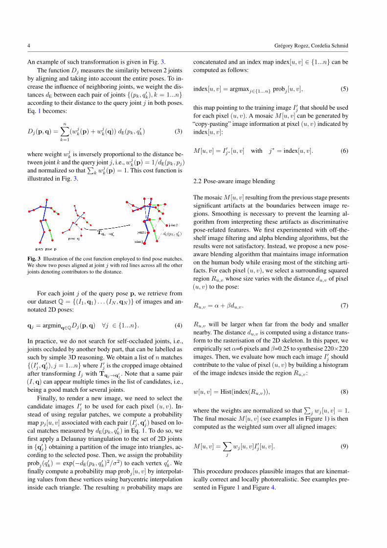
An example of such transformation is given in Fig. 3.The function Dj measures the similarity between 2 joints
by aligning and taking into account the entire poses. To in-crease the influence of neighboring joints, we weight the dis-tances dE between each pair of joints {(pk, q′k), k = 1...n}according to their distance to the query joint j in both poses.Eq. 1 becomes:
Dj(p,q) =
n∑
k=1
(wjk(p) + wj
k(q)) dE(pk, q′k) (3)
where weight wjk is inversely proportional to the distance be-
tween joint k and the query joint j, i.e.,wjk(p) = 1/dE(pk, pj)
and normalized so that∑
k wjk(p) = 1. This cost function is
illustrated in Fig. 3.
Fig. 3 Illustration of the cost function employed to find pose matches.We show two poses aligned at joint j with red lines across all the otherjoints denoting contributors to the distance.
For each joint j of the query pose p, we retrieve fromour dataset Q = {(I1,q1) . . . (IN ,qN )} of images and an-notated 2D poses:
qj = argminq∈QDj(p,q) ∀j ∈ {1...n}. (4)
In practice, we do not search for self-occluded joints, i.e.,joints occluded by another body part, that can be labelled assuch by simple 3D reasoning. We obtain a list of n matches{(I ′j ,q′j), j = 1...n} where I ′j is the cropped image obtainedafter transforming Ij with Tqj→q′j
. Note that a same pair(I,q) can appear multiple times in the list of candidates, i.e.,being a good match for several joints.
Finally, to render a new image, we need to select thecandidate images I ′j to be used for each pixel (u, v). In-stead of using regular patches, we compute a probabilitymap pj [u, v] associated with each pair (I ′j ,q
′j) based on lo-
cal matches measured by dE(pk, q′k) in Eq. 1. To do so, we
first apply a Delaunay triangulation to the set of 2D jointsin {q′j} obtaining a partition of the image into triangles, ac-cording to the selected pose. Then, we assign the probabilityprobj(q
′k) = exp(−dE(pk, q
′k)
2/σ2) to each vertex q′k. Wefinally compute a probability map probj [u, v] by interpolat-ing values from these vertices using barycentric interpolationinside each triangle. The resulting n probability maps are
concatenated and an index map index[u, v] ∈ {1...n} can becomputed as follows:
index[u, v] = argmaxj∈{1...n} probj [u, v], (5)
this map pointing to the training image I ′j that should be usedfor each pixel (u, v). A mosaic M [u, v] can be generated by“copy-pasting” image information at pixel (u, v) indicated byindex[u, v]:
M [u, v] = I ′j∗ [u, v] with j∗ = index[u, v]. (6)
2.2 Pose-aware image blending
The mosaicM [u, v] resulting from the previous stage presentssignificant artifacts at the boundaries between image re-gions. Smoothing is necessary to prevent the learning al-gorithm from interpreting these artifacts as discriminativepose-related features. We first experimented with off-the-shelf image filtering and alpha blending algorithms, but theresults were not satisfactory. Instead, we propose a new pose-aware blending algorithm that maintains image informationon the human body while erasing most of the stitching arti-facts. For each pixel (u, v), we select a surrounding squaredregion Ru,v whose size varies with the distance du,v of pixel(u, v) to the pose:
Ru,v = α+ βdu,v. (7)
Ru,v will be larger when far from the body and smallernearby. The distance du,v is computed using a distance trans-form to the rasterisation of the 2D skeleton. In this paper, weempirically setα=6 pixels and β=0.25 to synthesise 220×220images. Then, we evaluate how much each image I ′j shouldcontribute to the value of pixel (u, v) by building a histogramof the image indexes inside the region Ru,v:
w[u, v] = Hist(index(Ru,v)), (8)
where the weights are normalized so that∑
j wj [u, v] = 1.The final mosaic M [u, v] (see examples in Figure 1) is thencomputed as the weighted sum over all aligned images:
M [u, v] =∑
j
wj [u, v]I′j [u, v]. (9)
This procedure produces plausible images that are kinemat-ically correct and locally photorealistic. See examples pre-sented in Figure 1 and Figure 4.

Image-based Synthesis for Deep 3D Human Pose Estimation 5
Fig. 4 Examples of synthetics images generated using Leeds Sport dataset (LSP)[23] and CMU motion capture dataset as 2D and 3D sourcesrespectively. For each case, we show the 2D pose overlaid on the image and the corresponding orientated 3D pose.
55 x
55
x 96
27 x
27
x 25
6
13 x
13
x 38
4
13 x
13
x 38
4
13 x
13
x 28
6
4096
4096 K
220 x 220
1
2
3
Top score 1 Top score 2 Top score 3
Fig. 5 CNN-based pose classifier. We show the different layers and their corresponding dimensions, with convolutional layers depicted in blueand fully connected ones in green. The output is a distribution over K pose classes. Pose estimation is obtained by taking the highest score in thisdistribution. We show on the right the 3D poses for 3 highest scores. For this example, the top scoring class (top score 1) is correct.
3 CNN for full-body 3D pose estimation
Human pose estimation has been addressed as a classifica-tion problem in the past [4,34,41,43]. Here, the 3D posespace is partitioned into K clusters and a K-way classifier istrained to return a distribution over pose classes. Such a clas-sification approach allows modeling multimodal outputs inambiguous cases, and produces multiple hypothesis that canbe rescored, e.g., using temporal information. Training sucha classifier requires a reasonable amount of data per classwhich implies a well-defined and limited pose space (e.g.walking action) [4,41], a large-scale synthetic dataset [43]or both [34]. Here, we introduce a CNN-based classificationapproach for full-body 3D pose estimation. Inspired by theDeepPose algorithm [60] where the AlexNet CNN architec-ture [27] is used for full-body 2D pose regression, we selectthe same architecture and adapt it to the task of 3D body
pose classification. This is done by adapting the last fully-connected layer to output a distribution of scores over poseclasses as illustrated in Figure 5. Training such a classifierrequires a large amount of training data that we generateusing our image-based synthesis engine.
Given a library of motion capture data and a set of cameraviews, we synthesize for each 3D pose a 220 × 220 image.This size has proved to be adequate for full-body pose estima-tion [60]. The 3D poses are then aligned with respect to thecamera center and translated to the center of the torso, i.e., theaverage position between shoulders and hips coordinates. Inthat way, we obtain orientated 3D poses that also contain theviewpoint information. We cluster the resulting 3D poses todefine our classes which will correspond to groups of similarorientated 3D poses, i.e., body pose configuration and cameraviewpoint. We empirically found that K=5000 clusters was

6 Grégory Rogez, Cordelia Schmid
Table 1 Impact of synthetic data on the performances for the regressor and the classifier. The 3D pose estimation results are given following theprotocol P1 of Human3.6M (see text for details).
Method Type 2D source 3D source Training Errorof images size size pairs (mm)
Reg. Real 17,000 17,000 17,000 112.9Class. Real 17,000 17,000 17,000 149.7Reg. Synth 17,000 190,000 190,000 101.9Class. Synth 17,000 190,000 190,000 97.2Reg. Real 190,000 190,000 190,000 139.6Class. Real 190,000 190,000 190,000 97.7Reg. Synth + Real 207,000 190,000 380,000 125.5Class. Synth + Real 207,000 190,000 380,000 88.1
a sufficient number of clusters and that adding more clustersdid not further improve the results. For evaluation, we returnthe average 2D and 3D poses of the top scoring class.
To compare with [60], we also train a holistic pose regres-sor, which regresses to 2D and 3D poses (not only 2D). To doso, we concatenate the 3D coordinates expressed in metersnormalized to the range [−1, 1], with the 2D pose coordinates,also normalized in the range [−1, 1] following [60].
4 Experiments
We address 3D pose estimation in the wild. However, theredoes not exist a dataset of real-world images with 3D annota-tions. We thus evaluate our method in two different settingsusing existing datasets: (1) we validate our 3D pose predic-tions using Human3.6M [20] which provides accurate 3D and2D poses for 15 different actions captured in a controlled in-door environment; (2) we evaluate on the Leeds Sport dataset(LSP) [23] that presents real-world images together withfull-body 2D pose annotations. We demonstrate competitiveresults with state-of-the-art methods for both of them.
Our image-based rendering engine requires two differenttraining sources: 1) a 2D source of images with 2D pose anno-tations and 2) a motion capture 3D source. We consider twodifferent datasets for each: for 3D poses we use the CMU mo-tion capture dataset1 and the Human3.6M 3D poses [20], andfor 2D pose annotations the MPII-LSP-extended dataset [38]and the Human3.6M 2D poses and images.Motion capture 3D source. The CMU motion capture datasetconsists of 2500 sequences and a total of 140,000 3D poses.We align the 3D poses w.r.t. the torso and select a subsetof 12,000 poses, ensuring that selected poses have at leastone joint 5 cm apart. In that way, we densely populate ourpose space and avoid repeating common poses, e.g., neu-tral standing or walking poses which are over-represented inthe dataset. For each of the 12,000 original motion captureposes, we sample 180 random virtual views with azimuthangle spanning 360 degrees and elevation angles in the range[−45, 45]. We generate over 2 million pairs of 3D/2D pose
1 http://mocap.cs.cmu.edu
configurations (articulated poses + camera position and an-gle). For Human3.6M, we randomly selected a subset of190,000 orientated 3D poses, discarding similar poses, i.e.,when the average Euclidean distance of the joints is less than15mm as in [67].2D source. For the training dataset of real images with 2Dpose annotations, we use the MPII-LSP-extended [38] whichis a concatenation of the extended LSP [24] and the MPIIdataset [3]. Some of the poses were manually corrected asa non-negligible number of annotations are not accurateenough or completely wrong (eg., right-left inversions orbad ordering of the joints along a limb). We mirror the im-ages to double the size of the training set, obtaining a total of80,000 images with 2D pose annotations. For Human3.6M,we consider the 4 cameras and create a pool of 17,000 im-ages and associated 2D poses that we also mirror. To create adiverse set of images, we ensure that the maximum joint-to-joint distance between corresponding 3D poses is over 5 cm,i.e., similar poses have at least one joint 5 cm apart in 3D.
4.1 Evaluation on Human3.6M Dataset
To compare our results with recent work in 3D pose esti-mation [67], we follow the protocol introduced in [26] andemployed in [67]: we consider six subjects (S1, S5, S6, S7,S8 and S9) for training, use every 64th frame of subject S11for testing and evaluate the 3D pose error (mm) averagedover the 13 joints. We refer to this protocol by P1. As in [67],we measure a 3D pose error that aligns the pose by a rigidtransformation, but we also report the absolute error.
We first evaluate the impact of our synthetic data on theperformances for both the regressor and classifier. The resultsare reported in Table 1. We can observe that when consideringfew training images (17,000), the regressor clearly outper-forms the classifier which, in turns, reaches better perfor-mances when trained on larger sets. This can be explained bythe fact that the classification approach requires a sufficientamount of examples. We, then, compare results when train-ing both regressor and classifier on the same 190,000 posesconsidering a) synthetic data generated from Human3.6M,

Image-based Synthesis for Deep 3D Human Pose Estimation 7
Fig. 6 Human 3.6M real and synthetic data. We show on the left a training image from protocol 2 with the overlayed 2D pose. In the middle, weshow a “mosaic” image synthetized using the 2D pose from the real image on the left. In this case, the mosaic has been built by stitching imagepatches from 3 different subjects. On the right, we show a synthetic “surreal” image obtained after rendering the SMPL model using the 3D posefrom the real image on the left. Note that for more realism, the surreal image is rendered at the exact same 3D location in the motion capture room,using the same camera and background as in the real image.
Table 2 Comparison with state-of-the-art methods on Human3.6Mfollowing protocol P1 that measures an aligned 3D pose distance.
Method 2D source 3D source Errorsize size (mm)
Bo&Sminchisescu [5] 120,000 120,000 117.9Kostrikov&Gall [26] 120,000 120,000 115.7
Iqbal et al. [67] 300,000 380,000 108.3Ours 207,000 190,000 88.1
b) the real images corresponding to the 190,000 poses andc) the synthetic and real images together. We observe that theclassifier has similar performance when trained on syntheticor real images, which means that our image-based renderingengine synthesizes useful data. Furthermore, we can see thatthe classifier performs much better when trained on syntheticand real images together. This means that our data is differentfrom the original data and allows the classifier to learn bet-ter features. Note that we retrain AlexNet from scratch. Wefound that it performed better than just fine-tuning a modelpre-trained on Imagenet (3D error of 88.1mm vs 98.3mmwith fine-tuning).
In Table 2, we compare our results to three state-of-the-artapproaches. Our best classifier, trained with a combination ofsynthetic and real data, outperforms these methods in termsof 3D pose estimation by a margin. Note that even thoughwe compute 3D pose error after 3D alignment, our methodinitially estimates absolute pose (with orientation w.r.t. thecamera). That is not the case of Bo et al. [5] for instance, whoestimate a relative pose and do not provide 3D orientation.Comparison with classical synthetic images. We make ad-ditional experiments to further understand how useful ourdata is with respect to more classical synthetic data, i.e. ob-tained by rendering a human 3D model as in [8,61]. To do so,we consider the same 190,000 poses from the previous exper-iments and render the SMPL 3D human mesh model [30] inthese exact same poses using the body parameters and texture
maps from [61]. To disambiguate the type of synthetic data,we refer to these new rendered images as “surreal” images, asnamed in [61] and refer to our data as “mosaic” images. Notethat for more realism and to allow for a better comparison,we place the 3D model in the exact same location withinthe Human3.6M capture room and use the backgrounds andcamera parameters of the corresponding views to render thescenes. An example of the resulting surreal images is visu-alized in Figure 6 where we also show the correspondingoriginal real image as well as our mosaic image obtained forthe exact same pose. When the 2D annotations are accurateand consistent, as it is the case with the Human3.6M dataset,our algorithm produces very plausible images that are locallyphotorealistic and kinematically correct without significantartefacts at the boundaries between the image patches. Notethat for this experiment, we use the poses and images fromsubjects S1, S5, S6, S7 and S8 to generate our synthetic sets,i.e. removing S9 from the training set. This allows us to alsoevaluate on a second protocol (P2) employed in [28,57,71]where only these 5 subjects are used for training.
We then performed quantitative evaluation by trainingthe same classifier on different combinations of the 3 types ofdata (real, mosaic and surreal). When combining 2 or 3 typesof data, we alternate the batches of each data type consideringthe exact same poses in the different batches. In practice, weconsider batches of 256 images and train for 80k iterations,i.e. 110, 55 and 37 epochs for respectively 1, 2 or 3 typesof data in the training set. We evaluate on the same subsetof frames from subject S11 that was used in the previousexperiments (protocol P1). The numerical results are given inFigure 7 where we report classification rate, absolute 3D poseerror and 3D pose error after alignment. We can observe thatthe model trained on real data (green plot) performs signifi-cantly worse than the model trained on our synthetic mosaics(blue) both in terms of classification and 3D pose errors. Witheven less real data available, subject S9 being removed from
8 Grégory Rogez, Cordelia Schmid
Classification rate (%)
3
9
16
23
30
iterations4000 28000 52000 76000
RealMosaicSurrealMosaic+RealReal+SurrealSurreal+MosaicReal+Surreal+Mosaic
Abs. 3D pose error (mm)
110
133
155
178
200
iterations4000 28000 52000 76000
3D pose error (mm)
85
99
113
126
140
iterations4000 28000 52000 76000
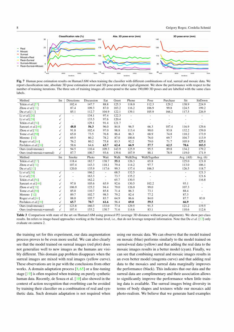
Fig. 7 Human pose estimation results on Human3.6M when training the classifier with different combinations of real, surreal and mosaic data. Wereport classification rate, absolute 3D pose estimation error and 3D pose error after rigid alignment. We show the performance with respect to thenumber of training iterations. The three sets of training images all correspond to the same 190,000 3D poses and are labelled with the same classlabels.
Method Im Directions Discussion Eat Greet Phone Pose Purchase Sit SitDownTekin et al.[57] 102.4 147.7 88.8 125.3 118.0 112.3 129.2 138.9 224.9Zhou et al.[71] 87.4 109.3 87.0 103.2 116.2 106.9 99.8 124.5 199.2Du et al.[12] 85.1 112.7 104.9 122.1 139.1 105.9 166.2 117.5 226.9Li et al.[28] X - 134.1 97.4 122.3 - - - - -Li et al.[29] X - 133.5 97.6 120.4 - - - - -Tekin et al.[56] X - 129.1 91.4 121.7 - - - - -Sanzari et al.[46] X 48.8 56.3 96.0 84.8 96.5 66.3 107.4 116.9 129.6Zhou et al.[70] X 91.8 102.4 97.0 98.8 113.4 90.0 93.8 132.2 159.0Tome et al.[58] X 65.0 73.5 76.8 86.4 86.3 68.9 74.8 110.2 173.9Moreno [32] X 69.5 80.2 78.2 87.0 100.8 76.0 69.7 104.7 113.9Rogez et al.[44] X 76.2 80.2 75.8 83.3 92.2 79.0 71.7 105.9 127.1Pavlakos et al.[36] X 58.6 64.6 63.7 62.4 66.9 57.7 62.5 78.6 103.5Ours (real+mosaic) X 94.5 110.4 109.3 143.9 125.9 95.5 89.8 134.2 179.2Ours (real+mosaic+surreal) X 87.7 100.7 93.6 139.6 107.9 88.1 78.9 119.0 171.9Method Im Smoke Photo Wait Walk WalkDog WalkTogether Avg. (All) Avg. (6)Tekin et al.[57] 118.4 182.7 138.7 55.1 126.3 65.8 125.0 121.0Zhou et al.[71] 107.4 143.3 118.1 79.4 114.2 97.7 113.0 106.1Du et al.[12] 120.0 135.9 117.6 99.3 137.4 106.5 126.5 118.7Li et al.[28] X - 166.2 - 68.5 132.5 - - 121.3Li et al.[29] X - 163.3 - 73.7 135.2 - - 121.6Tekin et al.[56] X - 162.2 - 65.7 130.5 - - 116.8Sanzari et al.[46] X 97.8 105.6 65.9 92.6 130.5 102.2 93.1 -Zhou et al.[70] X 106.9 125.2 94.4 79.0 126.0 99.0 107.3 -Tome et al.[58] X 85.0 110.7 85.8 71.4 86.3 73.1 88.4 -Moreno [32] X 89.7 102.7 98.5 79.2 82.4 77.2 87.3 -Rogez et al.[44] X 88.0 105.7 83.7 64.9 86.6 84.0 87.7 83.0Pavlakos et al.[36] X 65.7 70.7 61.6 56.4 69.0 59.5 66.9 -Ours (real+mosaic) X 123.8 160.3 133.0 77.4 129.5 91.3 121.2 119.5Ours (real+mosaic+surreal) X 107.4 155.2 130.7 71.6 114.6 83.1 110.6 112.6
Table 3 Comparison with state of the art on Human3.6M using protocol P2 (average 3D distance without pose alignment). We show per-classresults. Im refers to image-based approaches working at the frame level, i.e., that do not leverage temporal information. Note that Du et al. [12] onlyevaluate on camera 2.
the training set for this experiment, our data augmentationprocess proves to be even more useful. We can also clearlysee that the model trained on surreal images (red plot) doesnot generalize well to new images as the humans are visi-bly different. This domain gap problem disappears when thesurreal images are mixed with real images (yellow curve).These observations are in par with the conclusions from otherworks. A domain adaptation process [8,65] or a fine-tuningstage [19] is often required when training on purely synthetichuman data. Recently, de Souza et al. [10] also showed in thecontext of action recognition that overfitting can be avoidedby training their classifier on a combination of real and syn-thetic data. Such domain adaptation is not required when
using our mosaic data. We can observe that the model trainedon mosaic (blue) performs similarly to the model trained onsurreal+real data (yellow) and that adding the real data to themosaic images results in a better model (cyan). Finally, wecan see that combining surreal and mosaic images results inan even better model (magenta curve) and that adding realdata to the mosaics and surreal data marginally improvesthe performance (black). This indicates that our data and thesurreal data are complimentary and their association allowsto significantly improve the performance when little train-ing data is available. The surreal images bring diversity interms of body shapes and textures while our mosaics addphoto-realism. We believe that we generate hard examples

Image-based Synthesis for Deep 3D Human Pose Estimation 9
2D 3D Number of Human3.6M Human3.6M Human3.6M LSPsource source training samples Abs Error (mm) Align. Error (mm) Error (pix) Error (pix)
Human3.6M Human3.6M 190,000 130.1 97.2 8.8 31.1MPII+LSP Human3.6M 190,000 248.9 122.1 17.3 20.7MPII+LSP CMU 190,000 320.0 150.6 19.7 22.4MPII+LSP CMU 2.106 216.5 138.0 11.2 13.8
Table 4 Pose error on LSP and Human3.6M using different 2D and 3D sources for rendering the mosaic images and considering different numbersof training samples, i.e., 3D poses and corresponding rendered images.
Fig. 8 2D pose error on LSP and Human3.6M using different pools of annotated images to generate 2 millions of mosaic training images (left),varying the number of mosaic training images (center) and considering different number of pose classes K (right). On this last plot, we also reportthe lower-bound (LB) on the 2D error, i.e., computed with the closest classes from ground-truth annotations.
where the symmetry of the body in terms of shape, color andclothing has not been imposed. This seems to help learningmore discriminative features.
In Table 3, we compare our results to state-of-the-art ap-proaches for the second protocol (P2) where all the framesfrom subjects S9 and S11 are used for testing (and only S1,S5, S6, S7 and S8 are used for training). Our best classifier,trained with a combination of synthetic (mosaic & surreal)and real data, outperforms recent approaches in terms of 3Dpose estimation for single frames, even methods such as Zhouet al. [71] who integrate temporal information. Note that ourmethod estimates absolute pose (including orientation w.r.t.the camera), which is not the case for other methods such asBo et al. [5], who estimate a relative pose and do not provide3D orientation. Only the most recent methods report a bet-ter performance [32,36,44,58]. They use accurate 2D jointdetectors [32,58] or rely on much more complex architec-ture [36,44] while we employ a simple AlexNet architectureand return a coarse pose estimate.
4.2 Evaluation on Leeds Sport Dataset (LSP)
We now train our pose classifier using different combinationsof training sources and use them to estimate 3D poses onimages captured in-the-wild, i.e., LSP. Since 3D pose evalua-tion is not possible on this dataset, we instead compare 2Dpose errors expressed in pixels and measure this error on thenormalized 220× 220 images following [71]. We compute
the average 2D pose error over the 13 joints on both LSP andHuman3.6M (see Table 4).
As expected, we observe that when using a pool of thein-the-wild images to generate the mosaic data, the perfor-mance increases on LSP and drops on Human3.6M, showingthe importance of realistic images for good performance in-the-wild and the lack of generability of models trained onconstrained indoor images. The error slightly increases inboth cases when using the same number (190,000) of CMU3D poses. The same drop was observed by [67] and can be ex-plained by the fact that by CMU data covers a larger portionsof the 3D pose space, resulting in a worse fit. The resultsimprove on both test sets when considering more poses andsynthetic images (2 millions). The larger drop in Abs 3Derror and 2D error compared to aligned 3D error means thata better camera view is estimated when using more syntheticdata. In all cases, the performance (in pixel) is lower on LSPthan on Human3.6M due to the fact that the poses observedin LSP are more different from the ones in the CMU motioncapture data. In Figure 8 , we visualize the 2D pose error onLSP and Human3.6M 1) for different pools of annotated 2Dimages, 2) varying the number of synthesized training imagesand 3) considering different number of pose classes K. Asexpected using a bigger set of annotated images improvesthe performance in-the-wild. Pose error converges both onLSP and Human3.6M when using 1.5 million of images;using more than K=5000 classes does not further improvethe performance. The lower-bound on the 2D error, i.e., com-puted with the closest classes from ground-truth annotations,

10 Grégory Rogez, Cordelia Schmid
Method Feet Knees Hips Hands Elbows Shoulder Head AllWei et al. [63] 6.6 5.3 4.8 8.6 7.0 5.2 5.3 6.2
Pishchulin et al. [38] 10.0 6.8 5.0 11.1 8.2 5.7 5.9 7.6Chen & Yuille [9] 15.7 11.5 8.1 15.6 12.1 8.6 6.8 11.5
Yang et al. [66] 15.5 11.5 8.0 14.7 12.2 8.9 7.4 11.5Ours (AlexNet) 19.1 13 4.9 21.4 16.6 10.5 10.3 13.8
Ours (VGG) 16.2 10.6 4.1 17.7 13.0 8.4 9.8 11.5
Table 5 State-of-the-art results on LSP. The 2D pose error in pixels is computed on the normalized 220× 220 images.
clearly decreases when augmenting the number K of classes.Smaller clusters and finer pose classes are considered whenincreasing K. However, the performance does not furtherincrease for larger values of K. The classes become proba-bly too similar, resulting in ambiguities in the classification.Another reasons for this observation could be the amountof training data available for each class that also decreaseswhen augmenting K.Performance with a deeper architecture. To further im-prove the performance, we also experiment with fine-tuninga VGG-16 architecture [53] for pose classification. By do-ing so, the average (normalized) 2D pose error decreasesby 2.3 pixels. In Table 5, we compare our results on LSP tothe state-of-the-art 2D pose estimation methods. Althoughour approach is designed to estimate a coarse 3D pose, itsperformances is comparable to recent 2D pose estimationmethods [9,66]. In Figure 9, we present some qualitative re-sults obtained with our method. For each image, we show the3D pose corresponding to the average pose of the top scoringclass, i.e., the highest peak in the distribution. The qualita-tive results in Figure 9 show that our algorithm correctlyestimates the global 3D pose. We also show some failurecases.Re-ranking. After a visual analysis of the results, we foundthat failures occur in two cases: 1) when the observed posedoes not belong to the motion capture training database,which is a limitation of purely holistic approaches (e.g., thereexists no motion capture 3D pose of a diver as in the secondexample on the last row in Figure 9), or 2) when there is a pos-sible right-left or front-back confusion. We observed that thislater case is often correct for subsequent top-scoring poses.For the experiments in Table 5 using a VGG architecture,the classification rate2 on LSP is only 21.4%, meaning thatthe classes are very similar and very hard to disambiguate.However, this classification rate reaches 48.5% when consid-ering the best of the 5 top scoring classes, re-ranked usingground truth, as depicted in Fig. 10. It even reaches 100%
when re-ranking the 1000 top scoring classes. i.e., 20% of theK=5000 classes. The 2D error lower bound (≈ 8.7 pixels)is reached when re-ranking the first 100 top scoring classes,only 2% of theK=5000 classes. This highlights a property ofour approach that can keep multiple pose hypotheses which
2 ground truth classes being obtained by assigning the ground truth2D pose to the closest cluster.
could be re-scored adequately, for instance, using temporalinformation in videos.
4.3 Discussion
We now analyse the limitations of the proposed method anddiscuss future research.Limitations of the method. In Fig. 11, we show more visualexamples of generated images with our approach before andafter blending. To better compare the images with/withoutblending, some close-ups are provided. In general, our image-based synthesis engine works well when poses and cameraviews are similar in the query pose and the annotated images.For instance, if the annotated images only include peopleobserved from the front, our engine will not produce accept-able images from side or top views. In the same way, if the2D source only contains standing persons, the engine willnot be able to synthesise an acceptable image of a sittingpose. If viewpoint and pose are similar in query and anno-tated images, several factors can influence the quality of thesynthesised images. We found three main reasons for failureand show an example of each case in Fig. 12: 1) the simi-larity in person’s morphology and clothing in the selectedimages, in the example given in Fig. 12a, stitching patches ofpersons wearing trousers or shorts leads to poor result. 2) the3D depth ambiguities, this inherent to the fact that matchingis performed in 2D and several 3D poses can correspond tothe same 2D pose (see Fig. 12b). 3) the quality of the 2Dannotations. While the “perfect” 2D poses from Human3.6Mled to very plausible images, this is not always the case formanual annotations of real images. If the 2D annotations arenot consistent or inaccurate, as it often happens with bodykeypoints such as hips or shoulders, this can results in asynthetic image of poor quality as depicted in Fig. 12c.Pose and views. A limitation of the proposed approach isthat it does not learn the statistics of human poses in realimages nor the typical views that can be found in real images.These are two presumably important cues. Ideally, one wouldwant to synthesise useful training images that better matchthe test conditions. This could be achieved by sampling froma prior distribution of poses and camera viewpoints insteadof randomly selecting them as done in this paper.Image mosaicing. Our mosaic images do not look realistic.While it seems to be more important for the problem at hand

Image-based Synthesis for Deep 3D Human Pose Estimation 11
Fig. 9 Qualitative results on LSP. We show for each image, the 3D pose corresponding to the top scoring class, i.e. the highest peak in thedistribution. We show correct 3D pose estimations (top 3 rows), imprecise pose estimation due to coarse discretization (fourth row) and typicalfailure cases (bottom row), corresponding to unseen poses or right-left and front-back confusions.
to be locally photorealistic as opposed to globally coherent,this is only true for the 3D pose estimation approaches whichwere tested in this paper, i.e., deep pipeline with regressionor classification objective on images centered on the human.The proposed data might not be appropriate to train moreadvanced approaches to 3D pose estimation based on a moreglobal reasoning such as [44] who jointly detect the humans
in a natural image and estimate their 3D poses. The proposedoptimization ignores image compatibility, which it could takeinto account in future work. If a big enough 2D source, i.e.,pool of annotated images, was available, one could constrainthe matching in a way that the smallest set of images isused for synthesis, resulting in more satisfactory syntheticimages. A new cost function could minimize not just the

12 Grégory Rogez, Cordelia Schmid
Cla
ssif.
Acc
urac
y (%
)
0
25
50
75
100
num. re-ranked classes1 10 100 1000
2D E
rror (
pix)
8
9
10
11
12
num. re-ranked classes1 10 100 1000
Fig. 10 Classification accuracy and 2D pose error on LSP when re-ranking the top scoring classes. To show the potential improvement of areranking stage, we report the performance when varying the number of top scoring classes re-ranked using ground truth annotations.
Fig. 11 Examples of synthetic images generated using LSP and MPII datasets and CMU motion capture dataset as 2D and 3D sources respectively.For each case, we show the image before (up) and after (bottom) blending with close-ups.
Pose-aware Human3.6M Human3.6M Human3.6M LSPBlending Abs Error (mm) Error (mm) Error (pix) Error (pix)
yes 320.0 150.6 19.7 22.4no 337.6 186.2 22.8 35.9
Table 6 Pose error on LSP and Human3.6M with and without blending stage. We compare the results obtained by the AlexNet architecture whentrained on 190,000 mosaic images synthesized using CMU motion capture 3D poses and MPII+LSP dataset as 3D and 2D sources respectively.
individual joint scores as a “unary” but also some “binary”cost that evaluates the match between pairs of joint matches,and also a prior term that encourages color and geometricconsistency/minimal images.
Image blending. In this work, we have proposed to solvethe lack of color and geometric consistency with a pose-aware blending algorithm that removes the artefacts at theboundaries between image regions while maintaining poseinformative edges on the person. In Table 6, we report the per-formance of the proposed approach without this image blend-ing step and show that this second step is actually necessary.The proposed blending function can seem rather heuristic.Another solution could be a GAN-style [16] image synthe-sis approach: given images and the probability maps, find agenerator to generate images that also defeat a discrimina-tive loss. The resulting images would probably look more
compelling and probably respect the overall image structurebetter (coherent body parts and background geometry). Thiswill be explored in future work. Another intriguing questionfor future research is whether and to what extent a similar ap-proach could generate synthetic videos with 3D annotations.
5 Conclusion
In this paper, we introduce an approach for creating a syn-thetic training dataset of “in-the-wild” images and their cor-responding 3D pose. Our algorithm artificially augments adataset of real images with new synthetic images showingnew poses and, importantly, with 3D pose annotations. Weshowed that CNNs can be trained on these artificially lookingimages and still generalize well to real images without re-

Image-based Synthesis for Deep 3D Human Pose Estimation 13
(a) (b) (c)
Fig. 12 Examples of failure cases for synthetic images generated using LSP and MPII datasets and CMU motion capture dataset as 2D and 3Dsources respectively. For each case, we show the image before (up) and after (bottom) blending with close-ups. We show failures due to differencesin clothing (a), 3D depth ambiguity (b) and inaccurate 2D pose annotations (c).
quiring any domain adaptation or fine-tuning stage. We trainan end-to-end CNN classifier for 3D pose estimation andshow that, with our synthetic training images, our methodoutperforms most published methods in terms of 3D pose es-timation in controlled environments while employing a muchsimpler architecture. We also demonstrated our approach onthe challenging task of estimating 3D body pose of humansin natural images (LSP). Finally, our experiments highlightthat 3D pose classification can outperform regression in thelarge data regime, an interesting and not necessarily intuitiveconclusion. In this paper, we have estimated a coarse 3Dpose by returning the average pose of the top scoring cluster.In future work, we will investigate how top scoring classescould be re-ranked and also how the pose could be refined.
Acknowledgments. This work was supported by the Euro-pean Commission under FP7 Marie Curie IOF grant (PIOF-GA-2012-328288) and partially supported by the ERC ad-vanced grant ALLEGRO and an Amazon Academic ResearchAward (AARA). We acknowledge the support of NVIDIAwith the donation of the GPUs used for this research. Wethank Dr Philippe Weinzaepfel for his help. We also thankthe anonymous reviewers for their comments and suggestionsthat helped improve the paper.
References
1. A. Agarwal and B. Triggs. Recovering 3D human pose frommonocular images. PAMI, 28(1):44–58, 2006.
2. I. Akhter and M. Black. Pose-conditioned joint angle limits for 3Dhuman pose reconstruction. In CVPR, 2015.
3. M. Andriluka, L. Pishchulin, P. Gehler, and B. Schiele. 2D humanpose estimation: New benchmark and state-of- the-art analysis. InCVPR, 2014.
4. A. Bissacco, M.-H. Yang, and S. Soatto. Detecting humans viatheir pose. In NIPS, 2006.
5. L. Bo and C. Sminchisescu. Twin Gaussian processes for structuredprediction. IJCV, 87(1-2):28–52, 2010.
6. L. Bourdev and J. Malik. Poselets: Body part detectors trainedusing 3D human pose annotations. In ICCV, 2009.
7. Ching-Hang Chen and Deva Ramanan. 3D human pose estimation= 2D pose estimation + matching. In CVPR, 2017.
8. W. Chen, H. Wang, Y. Li, H. Su, Z. Wang, C. Tu, D. Lischin-ski, D. Cohen-Or, and B. Chen. Synthesizing training images forboosting human 3D pose estimation. In 3DV, 2016.
9. X. Chen and A. L. Yuille. Articulated pose estimation by a graph-ical model with image dependent pairwise relations. In NIPS,2014.
10. C. R. de Souza, A. Gaidon, Y. Cabon, and A.M. Lopez. Proceduralgeneration of videos to train deep action recognition networks. InCVPR, 2017.
11. A. Dosovitskiy, P. Fischer, E. Ilg, P. Häusser, C. Hazirbas,V. Golkov, P. van der Smagt, D. Cremers, and T. Brox. Flownet:Learning optical flow with convolutional networks. In ICCV, 2015.
12. Y. Du, Y. Wong, Y. Liu, F. Han, Y. Gui, Z. Wang, M. Kankan-halli, and W. Geng. Marker-less 3D human motion capture withmonocular image sequence and height-maps. In ECCV, 2016.
13. A. Elhayek, E. Aguiar, A. Jain, J. Tompson, L. Pishchulin, M. An-driluka, C. Bregler, B. Schiele, and C. Theobalt. Efficient convnet-based marker-less motion capture in general scenes with a lownumber of cameras. In CVPR, 2015.
14. M. Enzweiler and D. M. Gavrila. A mixed generative-discriminative framework for pedestrian classification. In CVPR,2008.
15. X. Fan, K. Zheng, Y. Zhou, and S. Wang. Pose locality constrainedrepresentation for 3D human pose reconstruction. In ECCV, 2014.
16. I.J. Goodfellow, J. Pouget-Abadie, M. Mirza, B. Xu, D. Warde-Farley, S. Ozair, A. C. Courville, and Y. Bengio. Generative adver-sarial nets. In NIPS, 2014.
17. H. Hattori, V. N. Boddeti, K. M. Kitani, and T. Kanade. Learningscene-specific pedestrian detectors without real data. In CVPR,2015.
18. A. Hornung, E. Dekkers, and L. Kobbelt. Character animationfrom 2D pictures and 3D motion data. ACM Trans. Graph., 26(1),2007.
19. S. Huang and D. Ramanan. Expecting the unexpected: Trainingdetectors for unusual pedestrians with adversarial imposters. InCVPR, 2017.
20. C. Ionescu, D. Papava, V. Olaru, and C. Sminchisescu. Hu-man3.6M: Large scale datasets and predictive methods for 3D
14 Grégory Rogez, Cordelia Schmid
human sensing in natural environments. PAMI, 36(7):1325–1339,2014.
21. M. Jaderberg, K. Simonyan, A. Vedaldi, and A. Zisserman. Readingtext in the wild with convolutional neural networks. IJCV, 116(1):1–20, 2016.
22. M. Jaderberg, K. Simonyan, A. Zisserman, and K. Kavukcuoglu.Spatial transformer networks. In NIPS, 2015.
23. S. Johnson and M. Everingham. Clustered pose and nonlinearappearance models for human pose estimation. In BMVC, 2010.
24. S. Johnson and M. Everingham. Learning effective human poseestimation from inaccurate annotation. In CVPR, 2011.
25. H. Joo, H. Liu, L. Tan, L. Gui, B. Nabbe, I. Matthews, T. Kanade,S. Nobuhara, and Y. Sheikh. Panoptic studio: A massively multi-view system for social motion capture. In ICCV, 2015.
26. I. Kostrikov and J. Gall. Depth sweep regression forests for esti-mating 3D human pose from images. In BMVC, 2014.
27. A. Krizhevsky, I. Sutskever, and G. E. Hinton. Imagenet classifica-tion with deep convolutional neural networks. In NIPS, 2012.
28. S. Li, W. Zhang, and A. B. Chan. Maximum-margin structuredlearning with deep networks for 3D human pose estimation. InICCV, 2015.
29. S. Li, W. Zhang, and A. B. Chan. Maximum-margin structuredlearning with deep networks for 3D human pose estimation. IJCV,2016.
30. M. Loper, N. Mahmood, J. Romero, G. Pons-Moll, and M. J. Black.SMPL: A skinned multi-person linear model. ACM Trans. Graphics(Proc. SIGGRAPH Asia), 34(6):248:1–248:16, 2015.
31. D. Mehta, H. Rhodin, D. Casas, P. Fua, O. Sotnychenko, W. Xu,and C. Theobalt. Monocular 3D human pose estimation in the wildusing improved CNN supervision. In 3D Vision (3DV), 2017.
32. F. Moreno-Noguer. 3D human pose estimation from a single imagevia distance matrix regression. In CVPR, 2017.
33. G. Mori and J. Malik. Recovering 3D human body configurationsusing shape contexts. PAMI, 28(7):1052–1062, 2006.
34. R. Okada and S. Soatto. Relevant feature selection for human poseestimation and localization in cluttered images. In ECCV, 2008.
35. D. Park and D. Ramanan. Articulated pose estimation with tinysynthetic videos. In CVPR ChaLearn Looking at People Workshop,2015.
36. G. Pavlakos, X. Zhou, K. G. Derpanis, and K. Daniilidis. Coarse-to-fine volumetric prediction for single-image 3D human pose. InCVPR, 2017.
37. X. Peng, B. Sun, K. Ali, and K. Saenko. Learning deep objectdetectors from 3D models. In ICCV, 2015.
38. L. Pishchulin, E. Insafutdinov, S. Tang, B. Andres, M. Andriluka,P. V. Gehler, and B. Schiele. DeepCut: Joint subset partition andlabeling for multi person pose estimation. CVPR, 2016.
39. L. Pishchulin, A. Jain, M. Andriluka, T. Thormählen, andB. Schiele. Articulated people detection and pose estimation: Re-shaping the future. In CVPR, 2012.
40. V. Ramakrishna, T. Kanade, and Y. Sheikh. Reconstructing 3Dhuman pose from 2D image landmarks. In ECCV, 2012.
41. G. Rogez, J. Rihan, C. Orrite, and P. Torr. Fast human pose de-tection using randomized hierarchical cascades of rejectors. IJCV,99(1):25–52, 2012.
42. G. Rogez and C. Schmid. MoCap-guided data augmentation for3D pose estimation in the wild. In NIPS, 2016.
43. G. Rogez, J. Supancic, and D. Ramanan. First-person pose recog-nition using egocentric workspaces. In CVPR, 2015.
44. G. Rogez, P. Weinzaepfel, and C. Schmid. LCR-Net: Localization-Classification-Regression for human pose. In CVPR, 2017.
45. J. Romero, H. Kjellstrom, and D. Kragic. Hands in action: Real-time 3D reconstruction of hands in interaction with objects. InICRA, 2010.
46. M. Sanzari, V. Ntouskos, and F. Pirri. Bayesian image based 3Dpose estimation. In ECCV, 2016.
47. G. Shakhnarovich, P. A. Viola, and T. Darrell. Fast pose estimationwith parameter-sensitive hashing. In ICCV, 2003.
48. J. Shotton, A. W. Fitzgibbon, M. Cook, T. Sharp, M. Finocchio,R. Moore, A. Kipman, and A. Blake. Real-time human pose recog-nition in parts from single depth images. In CVPR, 2011.
49. L. Sigal, A. O. Balan, and M. J. Black. Humaneva: Synchronizedvideo and motion capture dataset and baseline algorithm for evalu-ation of articulated human motion. IJCV, 87(1-2):4–27, 2010.
50. L. Sigal and M. J. Black. Predicting 3D people from 2D pictures.In AMDO, 2006.
51. E. Simo-Serra, A. Quattoni, C. Torras, and F. Moreno-Noguer. Ajoint model for 2D and 3D pose estimation from a single image. InCVPR, 2013.
52. E. Simo-Serra, A. Ramisa, G. Alenyà, C. Torras, and F. Moreno-Noguer. Single image 3D human pose estimation from noisyobservations. In CVPR, 2012.
53. K. Simonyan and A. Zisserman. Very deep convolutional networksfor large-scale image recognition. CoRR, abs/1409.1556, 2014.
54. H. Su, C. Ruizhongtai Qi, Y. Li, and L. J. Guibas. Render for CNN:viewpoint estimation in images using CNNs trained with rendered3D model views. In ICCV, 2015.
55. Camillo J. Taylor. Reconstruction of articulated objects from pointcorrespondences in a single uncalibrated image. In CVPR, 2000.
56. B. Tekin, I. Katircioglu, M. Salzmann, V. Lepetit, and P. Fua. Struc-tured prediction of 3D human pose with deep neural networks. InBMVC, 2016.
57. B. Tekin, A. Rozantsev, V. Lepetit, and P. Fua. Direct predictionof 3D body poses from motion compensated sequences. In CVPR,2016.
58. D. Tome, C. Russell, and L. Agapito. Lifting from the deep: Con-volutional 3D pose estimation from a single image. In CVPR,2017.
59. J. J. Tompson, A. Jain, Y. LeCun, and C. Bregler. Joint trainingof a convolutional network and a graphical model for human poseestimation. In NIPS, 2014.
60. A. Toshev and C. Szegedy. DeepPose: Human pose estimation viadeep neural networks. In CVPR, 2014.
61. G. Varol, J. Romero, X. Martin, N. Mahmood, M.J. Black, I. Laptev,and C. Schmid. Learning from synthetic humans. In CVPR, 2017.
62. C. Wang, Y. Wang, Z. Lin, A. L. Yuille, and W. Gao. Robustestimation of 3D human poses from a single image. In CVPR,2014.
63. S-E Wei, V. Ramakrishna, T. Kanade, and Y. Sheikh. Convolutionalpose machines. In CVPR, 2016.
64. Z. Wu, S. Song, A. Khosla, F. Yu, L. Zhang, X. Tang, and J. Xiao.3D shapenets: A deep representation for volumetric shapes. InCVPR, 2015.
65. J. Xu, S. Ramos, D.Vázquez, and A. M. López. Domain adaptationof deformable part-based models. PAMI, 36(12):2367–2380, 2014.
66. W. Yang, W. Ouyang, H. Li, and X. Wang. End-to-end learn-ing of deformable mixture of parts and deep convolutional neuralnetworks for human pose estimation. In CVPR, 2016.
67. H. Yasin, U. Iqbal, B. Krüger, A. Weber, and J. Gall. A dual-sourceapproach for 3D pose estimation from a single image. In CVPR,2016.
68. F. Zhou and F. De la Torre. Spatio-temporal matching for humandetection in video. In ECCV, 2014.
69. X. Zhou, Q. Huang, X. Sun, X. Xue, and Y. Wei. Towards 3Dhuman pose estimation in the wild: A weakly-supervised approach.In ICCV, 2017.
70. X. Zhou, X. Sun, W. Zhang, S. Liang, and Y. Wei. Deep kinematicpose regression. In ECCV Workshop on Geometry Meets DeepLearning, 2016.
71. X. Zhou, M. Zhu, S. Leonardos, K. Derpanis, and K. Daniilidis.Sparseness meets deepness: 3D human pose estimation frommonocular video. In CVPR, 2016.
72. S. Zuffi and M. J. Black. The stitched puppet: A graphical modelof 3D human shape and pose. In CVPR, 2015.