Image Colorization usingGenerative Adversarial Networks

Kamyar Nazeri, Eric Ng, and Mehran Ebrahimi

Faculty of Science, University of Ontario Institute of Technology2000 Simcoe Street North, Oshawa, Ontario, Canada L1H 7K4

{kamyar.nazeri,eric.ng,mehran.ebrahimi}@uoit.ca

http://www.ImagingLab.ca/

Abstract. Over the last decade, the process of automatic image col-orization has been of significant interest for several application areasincluding restoration of aged or degraded images. This problem is highlyill-posed due to the large degrees of freedom during the assignment ofcolor information. Many of the recent developments in automatic col-orization involve images that contain a common theme or require highlyprocessed data such as semantic maps as input. In our approach, weattempt to fully generalize the colorization procedure using a condi-tional Deep Convolutional Generative Adversarial Network (DCGAN).The network is trained over datasets that are publicly available such asCIFAR-10 and Places365. The results between the generative model andtraditional deep neural networks are compared.

1 Introduction

The automatic colorization of grayscale images has been an active area of re-search in machine learning for an extensive period of time. This is due to thelarge variety of applications such color restoration and image colorization foranimations. In this manuscript, we will explore the method of colorization usinggenerative adversarial networks (GANs) proposed by Goodfellow et al. [1]. Thenetwork is trained on the datasets CIFAR-10 and Places365 [2] and its resultswill be compared with those obtained using existing convolutional neural net-works (CNN).Models for the colorization of grayscales began back in the early 2000s. In 2002,Welsh et al. [3] proposed an algorithm that colorized images through texturesynthesis. Colorization was done by matching luminance and texture informa-tion between an existing color image and the grayscale image to be colorized.However, this proposed algorithm was defined as a forward problem, thus all so-lutions were deterministic. Levin et al. [4] proposed an alternative formulation tothe colorization problem in 2004. This formulation followed an inverse approach,where the cost function was designed by penalizing the difference between eachpixel and a weighted average of its neighboring pixels. Both of these proposedmethods still required significant user intervention which made the solutions lessthan ideal.

arX

iv:1

803.

0540

0v5

[cs

.CV

] 1

6 M

ay 2

018

In [5], a colorization method was proposed by comparing colorization differencesbetween those generated by convolutional neural networks and GAN. The mod-els in the study not only learn the mapping from input to output image, butalso learn a loss function to train this mapping. Their approach was effective inill-posed problems such as synthesizing photos from label maps, reconstructingobjects from edge maps, and colorizing images. We aim to extend their approachby generalizing the colorization procedure to high resolution images and suggesttraining strategies that speed up the process and greatly stabilize it.

2 Generative Adversarial Network

In 2014, Goodfellow et al. [1] proposed a new type of generative model: genera-tive adversarial networks (GANs). A GAN is composed of two smaller networkscalled the generator and discriminator. As the name suggests, the generator’stask is to produce results that are indistinguishable from real data. The discrim-inator’s task is to classify whether a sample came from the generator’s modeldistribution or the original data distribution. Both of these subnetworks aretrained simultaneously until the generator is able to consistently produce resultsthat the discriminator cannot classify.The architectures of the generator and discriminator both follow a multilayerperceptron model. Since colorization is a class of image translation problems,the generator and discriminator are both convolutional neural networks (CNNs).The generator is represented by the mapping G(z; θG), where z is a noise vari-able (uniformly distributed) that acts as the input of the generator. Similarly,the discriminator is represented by the mapping D(x; θD) to produce a scalarbetween 0 and 1, where x is a color image. The output of the discriminator canbe interpreted as the probability of the input originating from the training data.These constructions of G and D enable us to determine the optimization prob-lem for training the generator and discriminator: G is trained to minimize theprobability that the discriminator makes a correct prediction in generated data,while D is trained to maximize the probability of assigning the correct label.Mathematically, this can be expressed as

minθG

J (G)(θD, θG) = minθG

Ez [log(1−D(G(z)))] , (1)

maxθD

J (D)(θD, θG) = maxθD

(Ex [log(D(x))] + Ez [log(1−D(G(z)))]) . (2)

The above two equations provide the cost functions required to train a GAN.In literature, these two cost functions are often presented as a single minimaxgame problem with the value function V (G,D):

minG

maxD

V (G,D) = Ex [logD(x)] + Ez [log(1−D(G(z)))] . (3)

In our model, we have decided to use an alternate cost function for the generator.In equation 1, the cost function is defined by minimizing the probability of the

2

discriminator being correct. However, this approach presents two issues: 1) Ifthe discriminator performs well during training stages, the generator will have anear-zero gradient during back-propagation. This will tremendously slow downconvergence rate because the generator will continue to produce similar resultsduring training. 2) The original cost function is a strictly decreasing functionthat is unbounded below. This will cause the cost function to diverge to −∞during the minimization process.To address the above issues, we have redefined the generator’s cost functionby maximizing the probability of the discriminator being mistaken, as opposedto minimizing the probability of the discriminator being correct. The new costfunction was suggested by Goodfellow at NIPS 2016 Tutorial [6] as a heuristic,non-saturating game, and is presented as:

maxθG

J (G)∗(θD, θG) = maxθG

Ez [log(D(G(z)))] , (4)

which can also be written as the minimization problem:

minθG−J (G)∗(θD, θG) = min

θG−Ez [log(D(G(z)))] . (5)

The comparison between the cost functions in equations 1 and 5 can be visualizedin figure 1 by the blue and red curves respectively. In addition, the cost function

Fig. 1: Comparison of cost functions J(G) (dashed blue) and −J(G)∗ (red).

was further modified by using the `1-norm in the regularization term [5]. Thisproduces an effect where the generator is forced to produce results that aresimilar to the ground truth images. This will theoretically preserve the structureof the original images and prevent the generator from assigning arbitrary colorsto pixels just to “fool” the discriminator. The cost function takes the form

minθG

J (G)∗(θD, θG) = minθG−Ez [log(D(G(z)))] + λ‖G(z)− y‖1 (6)

where λ is a regularization parameter and y is the ground truth color labels.

3

2.1 Conditional GAN

In a traditional GAN, the input of the generator is randomly generated noisedata z. However, this approach is not applicable to the automatic colorizationproblem because grayscale images serve as the inputs of our problem rather thannoise. This problem was addressed by using a variant of GAN called conditionalgenerative adversarial networks [7]. Since no noise is introduced, the input ofthe generator is treated as zero noise with the grayscale input as a prior, ormathematically speaking, G(0z|x). In addition, the input of the discriminatorwas also modified to accommodate for the conditional network. By introducingthese modifications, our final cost functions are as follows:

minθG

J (G)(θD, θG) = minθG−Ez [log(D(G(0z|x)))] + λ‖G(0z|x)− y‖1 (7)

maxθD

J (D)(θD, θG) = maxθD

(Ey [log(D(y|x))] + Ez [log(1−D(G(0z|x)|x))]) (8)

The discriminator gets colored images from both generator and original dataalong with the grayscale input as the condition and tries to decide which paircontains the true colored image.

3 Method

Image colorization is an image-to-image translation problem that maps a highdimensional input to a high dimensional output. It can be seen as pixel-wiseregression problem where structure in the input is highly aligned with structurein the output. That means the network needs not only to generate an output withthe same spatial dimension as the input, but also to provide color informationto each pixel in the grayscale input image. We provide an entirely convolutionalmodel architecture using a regression loss as our baseline and then extend theidea to adversarial nets.In this work we utilize the L*a*b* color space for the colorization task. This isbecause L*a*b* color space contains dedicated channel to depict the brightnessof the image and the color information is fully encoded in the remaining twochannels. As a result, this prevents any sudden variations in both color andbrightness through small perturbations in intensity values that are experiencedthrough RGB.

3.1 Baseline Network

For our baseline model, we follow the “fully convolutional network”[8] modelwhere the fully connected layers are replaced by convolutional layers which in-clude upsampling instead of pooling operators. This idea is based on encoder-decoder networks [9] where input is progressively downsampled using a series ofcontractive encoding layers, and then the process is reversed using a series ofexpansive decoding layers to reconstruct the input. Using this method we can

4

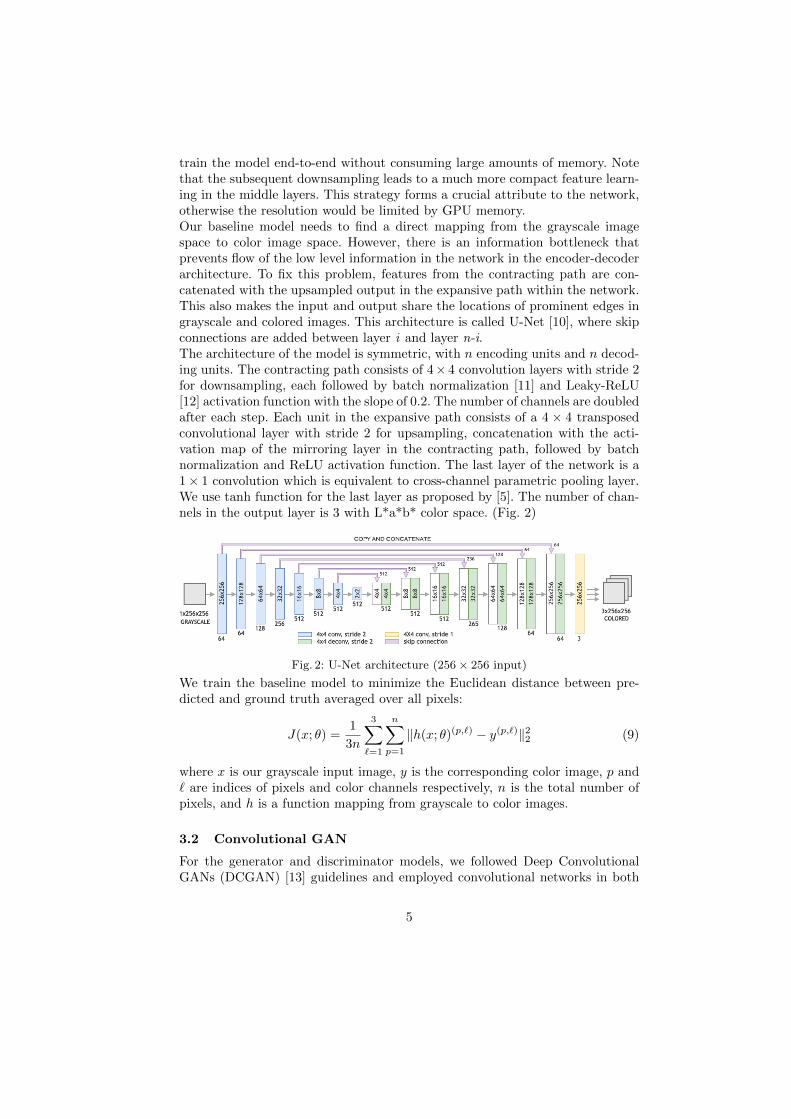
train the model end-to-end without consuming large amounts of memory. Notethat the subsequent downsampling leads to a much more compact feature learn-ing in the middle layers. This strategy forms a crucial attribute to the network,otherwise the resolution would be limited by GPU memory.Our baseline model needs to find a direct mapping from the grayscale imagespace to color image space. However, there is an information bottleneck thatprevents flow of the low level information in the network in the encoder-decoderarchitecture. To fix this problem, features from the contracting path are con-catenated with the upsampled output in the expansive path within the network.This also makes the input and output share the locations of prominent edges ingrayscale and colored images. This architecture is called U-Net [10], where skipconnections are added between layer i and layer n-i.The architecture of the model is symmetric, with n encoding units and n decod-ing units. The contracting path consists of 4× 4 convolution layers with stride 2for downsampling, each followed by batch normalization [11] and Leaky-ReLU[12] activation function with the slope of 0.2. The number of channels are doubledafter each step. Each unit in the expansive path consists of a 4 × 4 transposedconvolutional layer with stride 2 for upsampling, concatenation with the acti-vation map of the mirroring layer in the contracting path, followed by batchnormalization and ReLU activation function. The last layer of the network is a1× 1 convolution which is equivalent to cross-channel parametric pooling layer.We use tanh function for the last layer as proposed by [5]. The number of chan-nels in the output layer is 3 with L*a*b* color space. (Fig. 2)

Fig. 2: U-Net architecture (256 × 256 input)

We train the baseline model to minimize the Euclidean distance between pre-dicted and ground truth averaged over all pixels:

J(x; θ) =1

3n

3∑`=1

n∑p=1

‖h(x; θ)(p,`) − y(p,`)‖22 (9)

where x is our grayscale input image, y is the corresponding color image, p and` are indices of pixels and color channels respectively, n is the total number ofpixels, and h is a function mapping from grayscale to color images.

3.2 Convolutional GAN

For the generator and discriminator models, we followed Deep ConvolutionalGANs (DCGAN) [13] guidelines and employed convolutional networks in both

5

generator and discriminator architectures. The architecture was also modified asa conditional GAN instead of a traditional DCGAN; we also follow guideline in[5] and provide noise only in the form of dropout [14], applied on several layersof our generator. The architecture of generator G is the same as the baseline. Fordiscriminator D, we use similar architecture as the baselines contractive path:a series of 4× 4 convolutional layers with stride 2 with the number of channelsbeing doubled after each downsampling. All convolution layers are followed bybatch normalization, leaky ReLU activation with slope 0.2. After the last layer,a convolution is applied to map to a 1 dimensional output, followed by a sigmoidfunction to return a probability value of the input being real or fake. The inputof the discriminator is a colored image either coming from the generator or truelabels, concatenated with the grayscale image.

3.3 Training Strategies

For training our network, we used Adam [15] optimization and weight initial-ization as proposed by [16]. We used initial learning rate of 2 × 10−4 for bothgenerator and discriminator and manually decayed the learning rate by a factorof 10 whenever the loss function started to plateau. For the hyper-parameter λwe followed the protocol from [5] and chose λ = 100, which forces the generatorto produce images similar to ground truth.GANs have been known to be very difficult to train as it requires finding a Nashequilibrium of a non-convex game with continuous, high dimensional parameters[17]. We followed a set of constraints and techniques proposed by [5,13,17,18] toencourage convergence of our convolutional GAN and make it stable to train.

– Alternative Cost FunctionThis heuristic alternative cost function [6] was selected due to its non-saturating nature; the motivation for this cost function is to ensure thateach player has a strong gradient when that player is “losing” the game.

– One Sided Label SmoothingDeep neural networks normally tend to produce extremely confident outputswhen used in classification. It is shown that replacing the 0 and 1 targetsfor a classifier with smoothed values, like .1 and .9 is an excellent regular-izer for convolutional networks [19]. Salimans et al [17] demonstrated thatone-sided label smoothing will encourage the discriminator to estimate softprobabilities and reduce the vulnerability of GANs to adversarial examples.In this technique we smooth only the positive labels to 0.9, leaving negativelabels set to 0.

– Batch NormalizationOne of the main difficulties when training GANs is for the generator tocollapse to a parameter setting where it always emits the same output [17].This phenomenon is called mode-collapse, also known as the Helveticascenario [6]. When mode-collapse has occurred, the generator learns that asingle output is able to consistently trick the discriminator. This is non-idealas the goal is for the network to learn the distribution of the data rather

6

than the most ideal way of fooling the discriminator. Batch normalization[11] is proven to be essential to train both networks preventing the generatorfrom collapsing all samples to a single point [13]. Batch-Norm is not appliedon the first layer of generator and discriminator and the last layer of thegenerator as suggested by [5].

– All Convolutional NetStrided convolutions are used instead of spatial pooling functions. This effec-tively allows the model to learn its own downsampling/upsampling ratherthan relying on a fixed downsampling/upsampling method. This idea wasproposed in [20] and has shown to improve training performance as the net-work learns all necessary invariances just with convolutional layers.

– Reduced MomentumWe use Adam optimizer [15] for training both networks. Recent research hasshown that using a large momentum term β1 (0.9 as suggested), could resultin oscillation and instability in training. We followed the suggestion in [13]to reduce the momentum term to 0.5.

– LeakyReLU Activation FunctionRadford et al. [13] showed that using leaky ReLU [5] activation functions inthe discriminator resulted in better performance over using regular ReLUs.We also found that using leaky ReLU in the encoder part of the generatoras suggested by [5] works slightly better.

4 Experimental Results

To measure the performance, we have chosen to employ mean absolute error(MAE) and accuracy. MAE is computed by taking the mean of the absoluteerror of the generated and source images on a pixel level for each color channel.Accuracy is measured by the ratio between the number of pixels that have thesame color information as the source and the total number of pixels. Any twopixels are considered to have the same color if their underlying color channelslie within some threshold distance ε. This is mathematically represented by

acc(x, y) =1

n

n∑p=1

3∏`=1

1[0,ε`](|h(x)(p,`) − y(p,`)|) (10)

where 1[0,ε`](x),x ∈ R denotes the indicator function, y is the correspondingcolor image, h is a function mapping from grayscale to color images, and ε` isa threshold distance used for each color channel. The training results for eachmodel are summarized in Table 1. Some of the preliminary results using theCIFAR-10 (32 × 32) dataset are shown in Appendix A. The images from GANhad a clear visual improvement than those generated by the baseline CNN. Theimages generated by GAN contained colors that were more vibrant whereas theresults from CNN suffered from a light hue. In some cases, the GAN was ableto nearly replicate the ground truth. However, one drawback was that the GANtends to colorize objects in colors that are most frequently seen. For example,

7

Dataset Network Batch Size EPOCHs MAE Accuracy ε = 2% Accuracy ε = 5%

CIFAR-10 U-Net 128 200 7.9 13.7 37.2%

CIFAR-10 GAN 128 200 5.1 24.1 65.5%

Places365 GAN 16 20 7.5 18.3 47.3 %

Table 1: Training results of baseline model and GAN.

many car images were colored red. This is most likely due to the significantlylarger number of images with red cars than images with cars of another color.The preliminary results using Places365 (256 × 256) are shown in AppendixB. We noticed that there were some instances of mis-colorization: regions ofimages that have high fluctuations are frequently colored green. This is likelycaused by the large number of grassland images in the training set, thus themodel leans towards green whenever it detects a region with high fluctuations inpixel intensity values. We also noticed that some colorized images experienced a“sepia effect” seen with CIFAR-10 under U-Net. This hue is evident especiallywith images with clear sky, where the color of the sky includes a strange colorgradient between blue and light yellow. We suspect that this was caused byinsufficient training, and will correct itself over time.

5 Conclusion and Future Work

In this study, we were able to automatically colorize grayscale images using GAN,to an acceptable visual degree. With the CIFAR-10 dataset, the model was ableto consistently produce better looking (qualitatively) images than U-Net. Manyof the images generated by U-Net had a brown-ish hue in the results known asthe “Sepia effect” across L*a*b* color space. This is due to the L2 loss functionthat was applied to the baseline CNN, which is known to cause a blurring effect.We obtained mixed results when colorizing grayscale images using the Places365dataset. Mis-colorization was a frequent occurrence with images containing highlevels of textured details. This leads us to believe that the model has identifiedthese regions as grass since many images in the training set contained leavesor grass in an open field. In addition, this network was not as well-trained asthe CIFAR-10 counterpart due to its significant increase in resolution (256×256versus 32×32) and the size of the dataset (1.8 million versus 50, 000). We expectthe results will improve if the network is trained further.We would also need to seek a better quantitative metric to measure performance.This is because all evaluations of image quality were qualitative in our tests.Thus, having a new or existing quantitative metric such as peak signal-to-noiseratio (PSNR) and root mean square error (RMSE) will enable a much morerobust process of quantifying performance.Source code is publicly available at:

https://github.com/ImagingLab/Colorizing-with-GANs

8

Acknowledgments This research was supported in part by an NSERC DiscoveryGrant for ME. The authors gratefully acknowledge the support of NVIDIA Corporationfor donation of GPUs through its Academic Grant Program.

References

1. Ian Goodfellow, Jean Pouget-Abadie, Mehdi Mirza, Bing Xu, David Warde-Farley,Sherjil Ozair, Aaron Courville, and Yoshua Bengio. Generative adversarial nets.In Advances in neural information processing systems, pages 2672–2680, 2014.

2. Bolei Zhou, Aditya Khosla, Agata Lapedriza, Antonio Torralba, and Aude Oliva.Places: An image database for deep scene understanding. 2016.

3. Tomihisa Welsh, Michael Ashikhmin, and Klaus Mueller. Transferring color togreyscale images. In ACM TOG, volume 21, pages 277–280, 2002.

4. Anat Levin, Dani Lischinski, and Yair Weiss. Colorization using optimization. InACM transactions on graphics (tog), volume 23, pages 689–694. ACM, 2004.

5. Phillip Isola, Jun-Yan Zhu, Tinghui Zhou, and Alexei A Efros. Image-to-imagetranslation with conditional adversarial networks. 2016.

6. Ian Goodfellow. Nips 2016 tutorial: Generative adversarial networks. 2016.7. Mehdi Mirza and Simon Osindero. Conditional generative adversarial nets. 2014.8. Jonathan Long, Evan Shelhamer, and Trevor Darrell. Fully convolutional networks

for semantic segmentation. In Proceedings of the IEEE Conference on ComputerVision and Pattern Recognition, pages 3431–3440, 2015.

9. Geoffrey E Hinton and Ruslan R Salakhutdinov. Reducing the dimensionality ofdata with neural networks. science, 313(5786):504–507, 2006.

10. Olaf Ronneberger, Philipp Fischer, and Thomas Brox. U-net: Convolutional net-works for biomedical image segmentation. In International Conference on MedicalImage Computing and Computer-Assisted Intervention. Springer, 2015.

11. Sergey Ioffe and Christian Szegedy. Batch normalization: Accelerating deep net-work training by reducing internal covariate shift. In International Conference onMachine Learning, 2015.

12. Andrew L Maas, Awni Y Hannun, and Andrew Y Ng. Rectifier nonlinearitiesimprove neural network acoustic models. In Proc. ICML, volume 30, 2013.

13. Alec Radford, Luke Metz, and Soumith Chintala. Unsupervised representationlearning with deep convolutional generative adversarial networks. 2015.

14. Nitish Srivastava, Geoffrey E Hinton, Alex Krizhevsky, Ilya Sutskever, and RuslanSalakhutdinov. Dropout: a simple way to prevent neural networks from overfitting.Journal of machine learning research, 15(1):1929–1958, 2014.

15. Diederik Kingma and Jimmy Ba. Adam: A method for stochastic optimization.16. Kaiming He, Xiangyu Zhang, Shaoqing Ren, and Jian Sun. Delving deep into

rectifiers: Surpassing human-level performance on imagenet classification. In Pro-ceedings of the IEEE international conference on computer vision, 2015.

17. Tim Salimans, Ian Goodfellow, Wojciech Zaremba, Vicki Cheung, Alec Radford,and Xi Chen. Improved techniques for training gans. In Advances in NeuralInformation Processing Systems, pages 2234–2242, 2016.

18. Antonia Creswell, Tom White, Vincent Dumoulin, Kai Arulkumaran, Biswa Sen-gupta, and Anil A Bharath. Generative adversarial networks: An overview. 2017.

19. Christian Szegedy, Vincent Vanhoucke, Sergey Ioffe, Jon Shlens, and ZbigniewWojna. Rethinking the inception architecture for computer vision. In Proceedingsof the IEEE Conference on Computer Vision and Pattern Recognition, 2016.

20. Jost Tobias Springenberg, Alexey Dosovitskiy, Thomas Brox, and Martin Ried-miller. Striving for simplicity: The all convolutional net. 2014.

9

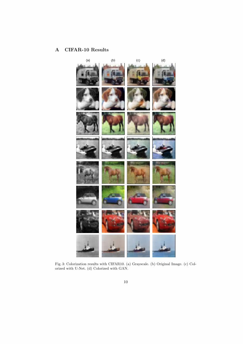
A CIFAR-10 Results

Fig. 3: Colorization results with CIFAR10. (a) Grayscale. (b) Original Image. (c) Col-orized with U-Net. (d) Colorized with GAN.

10

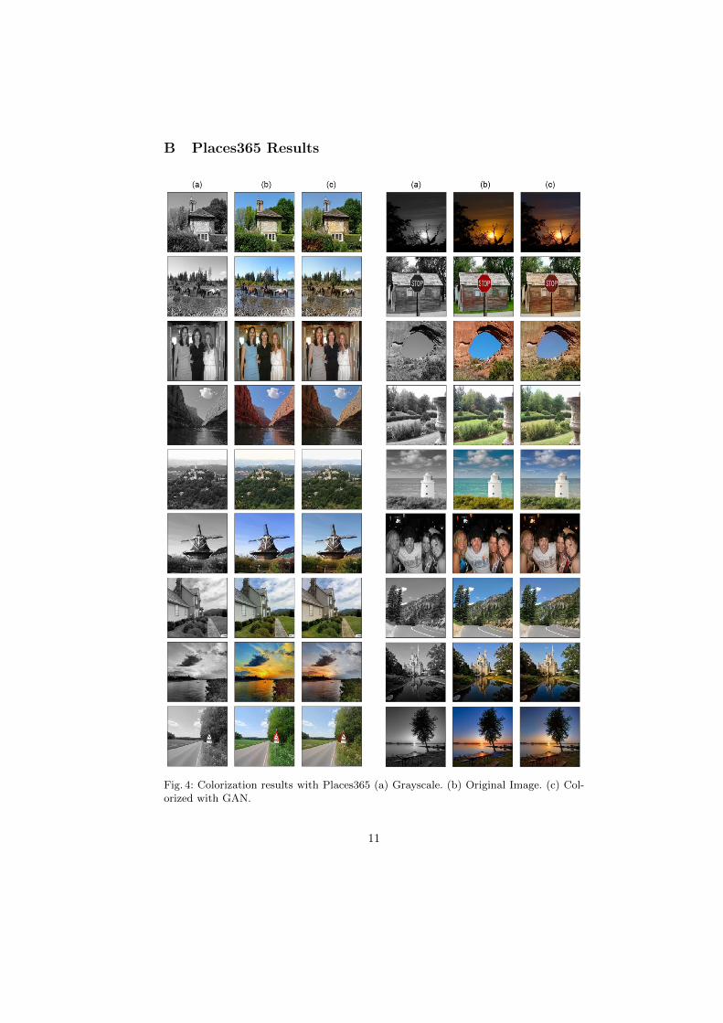
B Places365 Results

Fig. 4: Colorization results with Places365 (a) Grayscale. (b) Original Image. (c) Col-orized with GAN.

11