image denoising using stochastic chaotic simulated annealing · simulated annealing lipo wang,...
TRANSCRIPT

Image Denoising Using Stochastic Chaotic Simulated Annealing
Lipo Wang, Leipo Yan, and Kim-Hui Yap
School of Electrical and Electronic Engineering, Nanyang Technological University Block S1, 50 Nanyang Avenue, Singapore 639798
Abstract. In this Chapter, we present a new approach to image denoising based on a novel optimization algorithm called stochastic chaotic simulated annealing. The original Bayesian framework of image denoising is reformulated into a constrained optimization problem using continuous relaxation labeling. To solve this optimiza- tion problem, we then use a noisy chaotic neural network (NCNN), which adds noise and chaos into the Hopfield neural network (HNN) to facilitate efficient searching and to avoid local minima. Experimental results show that this approach can offer good quality solutions to image denoising.
Keywords: image denoising, neural networks, chaos, noise
1 Introduction
Image denoising is to estimate the original image from a noisy image with some assumptions or knowledge of the image degradation process. There exist many approaches for image denoising [I] [2] [3] [4]. Here we adopt a Bayesian framework because it is highly parallel and it can decompound a complex com- putation into a network of simple local computations [3], which is important in hardware implementation of neural networks. This approach computes the maximum a posteriori (MAP) estimation of the original image given a noisy image. The MAP estimation requires the prior distribution of the original im- age and the conditional distribution of the data. The prior distribution of the original images imposes contextual constraints and can be modeled by Markov random field (MRF) or, equivalently, by Gibbs distribution. The MAP-MRF principle centers on applying MAP estimation on MRF modeling of images.
Li incorporated augmented Lagrange multipliers into the Hopfield neural network (HNN) for solving optimization problems [5 ] . He transformed a com- binatorial optimization problem into real constrained optimization using the notion of continuous relaxation labeling. The HNN was then used to solve the real constrained optimization.

The neural network approaches have been shown to be a powerful tool for solving the optimization problems [6] [7]. The HNN is a typical model of neural network with symmetric connection weights. It is capable of solv- ing quadratic optimization problems. However, it suffers from convergence to local minima [8]. To overcome the weakness, different simulated annealing techniques have been combined with the HNN to solve optimization prob- lems [8] [9] [lo] [ll] [12]. Kajiura et a1 [ll] proposed the gaussian machine which combines stochastic simulated annealing (SSA) with neural network for solving assignment problems. Convergence to globally optimal solutions is guaranteed if the cooling schedule is sufficiently slow, i.e., no faster than logarithmic progress [3]. SSA searches the entire solution space, which is time consuming. Chen and Aihara [9] proposed a transiently chaotic neural net- work (TCNN) which adds a large negative self-coupling with slow damping in the Euler approximation of the continuous HNN so that neurodynamics eventually converge from strange attractors to an equilibrium point. Chaotic simulated annealing (CSA) can search efficiently because of its reduced search spaces. The TCNN showed good performance in solving traveling salesman problem. However CSA is deterministic and is not guaranteed to settle into a global minimum. In view of this, Wang and Tian [12] proposed a novel algo- rithm called stochastic chaotic simulated annealing (SCSA) which combines both stochastic manner of SSA and chaotic manner of CSA. In this paper the NCNN, which performs SCSA algorithm, is applied to solve the constrained optimization in the MAP-MRF formulated image denoising. Experimental results show that the NCNN outperforms the HNN and the TCNN.
The rest of the chapter is organized as follows: Section 2 introduces the MAP-MRF framework in image restoration and the transformation of the combinatorial optimization to a real unconstrained optimization. Section 3 presents the NCNN and the derivation of the neural network dynamics. The experimental results are shown in Section 4. Section 5 concludes the paper.
2 MAP-MRF Image Restoration
Let the original image, the restored image and the degraded image be denoted by x = {xi I i E S), f = {f i I i E S) and y = {yi I i E S) respectively, where S = {I,. . . , N) indexes the set of sites corresponding to the image pixels and N is the number of the image pixels.
When the original image is degraded by identical independently dis- tributed (i.i.d.) Gaussian noise, the degraded image is modeled by
where ei N N(0,a2) is the zero mean Gaussian distribution with standard deviation a . The objective of image denoising is to find an f that approximates 2.

Each pixel takes on a discrete value in the label set L = 1,. . . , M. The spatial relationship of the sites is determined by a neighborhood system N = {Ni I i E S) where Ni is the set of sites neighboring i. A single site or a set of neighboring sites form a clique denoted by c. C is the set of all cliques.
There are many different ways the pixels can influence each other through contextual interactions. Such contextual interactions can be modeled as MRFs. According to Markov-Gibbs equivalence [13], an MRF is equivalent to a Gibbs distribution
p(,) = 2 - 1 x e-+ C c c c v~(x) (2)
where V,(x) is the clique potential function, T is a temperature constant, and Z is a normalizing constant.
In the MAP-MRF labeling, the posterior distribution can be computed by using [14]
p(y) is a constant when y is given. P(x) is the prior probability and p(y1x) is the conditional distribution. The prior distribution of the original image which imposes the contextual constraints can be expressed in terms of the MRF clique potentials
where
In this chapter only pair-site cliques are considered. In (1) the noise is independent Gaussian noise. The conditional distribution
can be expressed in terms of y, x and a.
where
Knowing the prior distribution and the conditional distribution, the energy in the posterior distribution is given by [4]
in which C{i,i,lEC V2(xi,xi,) is the pair-site clique potential of the MRF model. Maximizing a posteriori is equivalent to find an 2 such that E(2) is the global minimum.

In order to minimize E(x) in (8), proper MRF model has to be chosen so that appropriate contextual constraints can be posed. Among various MRFs, the multi-level logistic (MLL) model is a simple mechanism for encoding a large class of spatial patterns [14]. In MLL, the pair-site clique potentials take the form
where PC is the parameter for cliques of type c = {i, il). However we found that the pair-site potentials are strong constraints. Instead of using (9) we use
Fig. 1. Graphical representation of g(xi, xi,)
g(xi, zit) in the modified potential function is an exponential function in (-1,1]. Compared to the potential function in the MLL model, the modified potential function allows the pixels to be slightly different from the neigh- boring pixels. This is logical as most real images have smooth non-uniform regions.
Since image pixels can only take discrete values, the minimization in (8) is combinatorial. The combinatorial optimization can be converted into a con- strained optimization in a real space using the continuous relaxation labeling. Let pi(I) E [O,1] represent the strength with which label I is assigned to i, the energy with the p variables is given by

where I = xi and I' = xi!, r i (I) = &(IIy) = ( I - yi)2/2a2 is the single- site clique potential function and r i , i~ ( I , 1') = V2(I, I' ly) = V2(I, 1') is the pair-site clique potential function in the posterior distribution P(x1y).
With such a representation, the combinatorial minimization is reformu- lated as the following constrained minimization
min E (p) P
(13)
subject to Ci(p) = 0 i E S (14)
pi(I) > 0 Vi E S , V I E L (15)
where Ci(p) = CIp i ( I ) - 1 = 0. The augmented Lagrange Hopfield (ALH) method can be used to solve the
above constrained minimization problem [4]. It uses the augmented Lagrange technique to satisfy the equality constraints of (14) and the Hopfield encoding to impose the inequality constraints of (15). The augmented Lagrange function takes the form
where yk are the Lagrange multipliers and P > 0 is the weight for the penalty term. The final solution p* is subject t o additional constraints: pf (I) E (0, 1).
The ALH method uses the HNN to optimize the energy function. However the HNN is prone to trappings at local minima. In view of this, we propose a new network NCNN to perform the optimization.
3 Noisy Chaotic Neural Network
Let ui(I) denote the internal state of the neuron (i, I ) and pi(I) denote the output of the neuron (i, I ) . pi(I) E [O,1] represents the strength that the pixel at location i takes the value I . The NCNN is formulated as follows [12]:

where TiI,ilIl : connection weight from neuron (i', It) to neuron (i, I ) ; Zi ( I ) : input bias of neuron (i, I ) ; k : damping factor of nerve membrane (0 5 k 5 1) a : positive scaling parameter for inputs; E : steepness parameter of the output function (E 2 0); z : self-feedback connection weight or refractory strength (z 2 0); I, : positive parameter; n : random noise injected into the neurons; p, : positive parameter (0 < ,B, < 1); ,& : positive parameter (0 < p, < 1); A[n] : the noise amplitude.
When n(t) in (18) equals to zero, the NCNN becomes TCNN. When dt) equals to zero, the TCNN becomes similar to the HNN with stable fixed point dynamics. The basic difference between the HNN and the TCNN is that a nonlinear term z( t ) (p i t ) (~) - I,) is added to the HNN. Since the "tempera- ture" dt) tends toward zero with time evolution, the updating equations of the TCNN eventually reduce to those of the HNN. In (18) the variable can be interpreted as the strength of negative self-feedback connection of each neuron, the damping of ~ ( ~ 1 produces successive bifurcations so that the neuro- dynamics eventually converge from strange attractors to a stable equilibrium point [8].
CSA is deterministic and is not guaranteed to settle into a global minimum. In view of this, Wang and Tian [12] added a noise term n(t) in (18). The noise term continues to search for the optimal solution after the chaos of the TCNN disappears.
From (13)-(15) and (18), we obtain the dynamics of the NCNN:
where
Note that the Lagrange multipliers are updated with neural outputs according to ,$+l) = (t) rk + PCi (P'" 1.
4 Experimental Results
Both artificial image and real image have been used to demonstrate the per- formance of the NCNN on image denoising.
The artificial image is a circle image of size 256 x 256 with M = 4 gray levels. Its label set is L = {0,1,2,3). Three noisy circle images were generated by adding zero-mean i.i.d. Gaussian noise with standard deviation a = 0.5, a = 0.75 and a = 1 respectively.

The noisy images were set to be the input of the neural networks. After the neural networks were initialized, each neuron was updated using (21) and (17). After all neurons in the neural networks were updated once, yk, z and n are updated. The updating scheme is cyclic and asynchronous. When all the neurons are updated once, we call it one iteration. Once the state of a neuron is updated, the new state information is immediately available to other neurons in the network (asynchronous).
The parameters that we used for the NCNN are: k = 1 , ~ = 0.01, a = 0.005, I. = 0.65, z(O) = 0.05, n(O) = 0.01. ,B is increased from 1 to 50 according to ,B c l . O l , B . The decreasing rate of z and n , ,LIZ and ,B, are 0.005. For the TCNN and the HNN we use the same parameters as the NCNN except that n = 0 for the TCNN, n = 0 and z = 0 for the HNN. The MRF pair-site clique potential parameter ,B,=l.
Table 1 shows the required iteration numbers and the peak signal-to-noise ratio (PSNR) of the denoised images. The higher the PSNR, the better the image quality. The denoised images are shown in Fig. 2-4.
Table 1. Numerical denoising results of the circle image (PSNRT: PSNR of the denoised image, PSNRd: PSNR of the noisy image)
Noise ~evell 11terationsI PSNR, I PSNRd I I HNN 1 23 135.8127118.70181
a = 0.5
a = 0.75
a = 1
The next experiment was conducted on the real image. The real image is the Lena image of size 128 x 128 with M = 256 gray levels. Its label set is L = {0,1,2,. . . ,255). Three noisy Lena images were generated by adding zero-mean i.i.d. Gaussian noise with standard deviation of a = 8, a = 16 and a = 24 respectively.
The denoising process of the noisy Lena images is the same as the circle image denoising process. The parameters that we used for the NCNN of the Lena image denoising process are: k = 1, E = 0.01, a = 0.0001, I. = 0.65, z(O) = 0.05, n(O) = 0.01. ,B is increased from 1 to 50 according to ,B t 1.01,B.
TCNN
NCNN
NCNN
HNN
TCNN
NCNN
HNN
TCNN
75
199
151
121
125
206
226
137
38.935
38.9675
29.4505
18.7018
18.7018
30.6347
33.0543
33.7814
27.3437
28.4625
14.7626
15.8694
15.8694
15.8694
14.7626
14.7626

Fig. 2. Denoising of the circle image with noise level u = 0.5: (a) Original image. (b) Noisy image. (c)-(e) Denoised images using the HNN, the TCNN and the NCNN, respectively

Fig. 3. Denoising of the circle image with noise level o = 0.75: (a) Original image. (b) Noisy image. (c)-(e) Denoised images using the HNN, the TCNN and the NCNN, respectively

Fig. 4. Denoising of the circle image with nose level a = 1: (a) Original image. (b) Noisy image. (c)-(e) Denoised images using the HNN, the TCNN and the NCNN, respectively

The decreasing rate of z and n, ,6, and ,6, are 0.005. For the TCNN and the HNN we use the same parameters as the NCNN except that n = 0 for the TCNN, n = 0 and z = 0 for the HNN. The MRF pair-site clique potential parameter PC=%
Table 2 shows the required iteration numbers and the peak signal-to-noise ratio (PSNR) of the denoised images. The higher the PSNR, the better the image quality. It can be seen from the table that the NCNN offers the best performance. The PSNR of the restored image using the NCNN is higher than those of the restored images using the HNN and the TCNN. In addition, the NCNN use less iterations to converge than the HNN and the TCNN. The denoised images are shown in Fig. 5-7.
Table 2. Numerical denoising results of the Lena image (PSNR,: PSNR of the denoised image, PSNRd: PSNR of the noisy image)
Noise ~evell I~terations
I HNN 1 950
HNN 1489
a = 1 6 TCNN 1173
NCNN 1114
HNN 2054
a = 24 TCNN 1571
NCNN 1862
5 Conclusion
A new neural network, called noisy chaotic neural network (NCNN), is used to address the MAP-MRF formulated image denoising problem. SCSA effectively overcomes the local minima problem. We have shown that the NCNN gives better quality solutions compared to the HNN and the TCNN.
References
1. Andrews, H. C., Hunt, B. R. (1977) Digital Image Restoration. Englewood Cliffs, N J, Prentice-Hall

Fig. 5. Denoising of the Lena Image with noise level a = 8: (a) Original image. (b) Noisy image. (c)-(e) Denoised images using the HNN, the TCNN and the NCNN, respectively
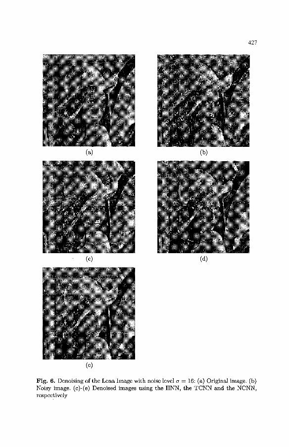
Fig. 6. Denoising of the Lena Image with noise level a = 16: (a) Original image. (b) Noisy image. (c)-(e) Denoised images using the HNN, the TCNN and the NCNN, respectively

Fig. 7. Denoising of the Lena Image with noise level a = 24: (a) Original image. (b) Noisy image. (c)-(e) Denoised images using the HNN, the TCNN and the NCNN, respectively

2. Rosenfeld, A., Kak, A. C. (1982) Digital Picture Processing, 1, Academic Press, 2nd edition
3. Geman ,S., Geman, D. (1984) Stochastic relaxation, gibbs distributions and the bayesian restoration of images. IEEE Transactions on Pattern Analysis and Machine Intelligence, 66, 721-741
4. Li, S. Z. (1998) Map image restoration and segmentation by constrained opti- mization. IEEE Transactions on Image Processing, 712, 1730-1735
5. Wang, H., Li, S. Z., Petrou, M. (1990) Relaxation labeling of markov random fields. IEEE Transactions on Systems, Man and Cybernetics, 20, 709-715
6. Peterson, C., Soderberg, B. (1992) Combinatorial Optimization with Neural Networks. Blackwell
7. Hopfield, J . J., Tank, D. W. (1985) Neural computation of decisions in opti- mization problems. Biol. Cybern., 52, 141-152
8. Chen, L., Aihara, K. (1995) Chaotic simulated annealing by a neural network model with transient chaos. Neural Networks, 86, 915-930
9. Chen, L., Aihara, K. (1994) Transient chaotic neural networks and chaotic sim- ulated annealing. Towards the Harness of Chaos, 347-352
10. Aihara, K., Tokuda, I., Nagashima, T . (1998) Adaptive annealing for chaotic optimization. Phys. Rev. El 58, 5157-5160
11. Kajiura, M., Anzai, Y., Akiyama, Y., Yamashira, A., Aiso, H. (1991) The gaus- sian machine: a stochastic neural network for solving assignment problems. J . Neural Network Comput., 2, 43-51
12. Wang, L., Tian, F. (2000) Noisy chaotic neural networks for solving combina- torial optimization problems. Proc. International Joint Conference on Neural Networks, 4, 4037-4040
13. Hammersley, J. M., Clifford, P. (1971) Markov field on finite graphs and lattices. unpublished Manuscript
14. Li, S. Z. (1995) Markov Random Field Modeling in Computer Vision. Springer- Verlag