Image Denoising Using Tree-based Wavelet SubbandCorrelations and Shrinkage

To appear in Optical Engineering

First author

James S. Walker

Department of Mathematics

University of Wisconsin–Eau Claire

Eau Claire, WI 54702–4004

Phone: 715–836–3301

Fax: 715–836–2924

e-mail: walkerjs@uwec.edu

Second author

Ying-Jui Chen

Department of Electrical

& Computer Engineering

Boston University

8 St Mary’s Street

Boston, MA 02215

Phone: 617-353-1040

Fax: 617-353-1282

e-mail: yrchen@bu.edu

Abstract

In this paper we describe new methods of denoising images which combine wavelet shrinkage withproperties related to the statistics of quad-trees of wavelet transform values for natural images.They are called Tree-Adapted Wavelet Shrinkage (TAWS) methods. The shift-averaged versionof TAWS produces denoisings which are comparable to state of the art denoising methods, suchas cycle-spin thresholding and the cycle-spin version of the Hidden Markov Tree method. Thenon-shift averaged version of TAWS is superior to the classic wavelet shrinkage method, and fitsnaturally into a signal compression algorithm. These TAWS methods bear some relation to therecently proposed Hidden Markov Tree methods, but are deterministic rather than probabilistic.They may prove useful in settings where speed is critical and/or signal compression is needed.

Keywords: image denoising; wavelet transform; signal processing.

1 Introduction

This paper describes a new method of denoising images called TAWS (Tree-Adapted WaveletShrinkage). The TAWS method is a modification of wavelet shrinkage, based upon a deterministicselection procedure for distinguishing image dominated wavelet transform values from noise dom-inated transform values. This selection procedure is adapted from a new image compression algo-rithm described in [1]. The TAWS algorithm is only slightly more complex than wavelet-shrinkage[2], yet yields superior denoisings. It has a shift-averaged version which yields denoisings com-parable or superior to state of the art denoising methods such as cycle-spin thresholding [3] anduHMT-spin [4].

The paper is organized as follows. In section 2, we describe the TAWS method. This sectionbegins with a brief summary of the compression method from which TAWS is derived. Under-standing the rationale behind this compression technique helps in understanding how TAWS com-bats the ringing artifacts that wavelet shrinkage suffers from. It also helps in understanding howTAWS dynamically adapts the sizes of thresholds in relation to specific image features. In section3, we report on denoisings of test images. A comparison of TAWS with various state of the artdenoising methods is done in this section. The paper concludes in section 4 with a brief discussionof future work.

2 The TAWS Method

The TAWS denoising method is built upon the ideas involved in a new lossy image codec calledAdaptively Scanned Wavelet Difference Reduction (ASWDR), which is described in [1]. Here isa summary of this method, with some amendments made to adapt to the noise removal case:

2

The ASWDR Method

Step 1. Perform a wavelet transform of the discrete image,����� ����� �

, producing the trans-formed image,

������ ����� �. For the denoisings reported on in this paper, the Daub 9/7 transform

[5] was used exclusively.

Step 2. Use a scanning order for searching through the transformed image. This is a one-to-one and onto mapping,

���� ����������� ��, whereby the transform values are scanned through via

a linear ordering�����

, � , . . . , � . The value of � being the number of pixels in the image.Initially, the scanning order is a zigzag through subbands, from lower to higher [6].

Step 3. Choose an initial threshold, � , such that at least one transform value,��� ��

say,satisfies � ��� �� � �!� and all transform values,

��� ��, satisfy � ��� �� � "#�$� .

Step 4 (Significance pass). Determine new significant index values—i.e., those new indices% for which��� %

has a magnitude greater than or equal to the present threshold. Assigna value & � % '� �)(�*,+�-/. ��� % 10

as the quantized value corresponding to the transform value��� % .

Step 5 (Refinement pass). Refine quantized transform values corresponding to old signifi-cant transform values. Each refined value is a better approximation to the exact transformvalue. More details of this step will be provided below.

Step 6. Create a new scanning order as follows. For the highest-scale level (the one con-taining the all-lowpass subband), use the indices of the remaining insignificant values as thescan order at that level. Use the scan order at level

�to create the new scan order at level�324�

as follows. Run through the significant values at level�

in the wavelet transform. Eachsignificant value, called a parent value, induces a set of four child values as described in thespatial-orientation tree definition in [7]. The first part of the scan order at level

�526�contains

the insignificant values lying among these child values. Run through the insignificant valuesat level

�in the wavelet transform. The second part of the scan order at level

�72��contains

the insignificant values lying among the child values induced by these insignificant parentvalues. Use this new scanning order for level

�324�to create the new scanning order for level�72 � , until all levels are exhausted. We shall explain the rationale for this step below.

Step 7. Divide the present threshold by � and repeat steps 4–7 until this new threshold is lessthan a preset value 8 .

A few remarks are in order to clarify the procedure outlined above. First, in the refinementpass, the precision of quantized values is increased to make them at least as accurate as the presentthreshold. For example, if an old significant transform’s magnitude � ��� % � lies in the interval� 9 � �;:=<=0 , say, and the present threshold is

<, then it will be decided at this step if its magnitude

lies in� 9 � �;:=>=0 or

� :=>?�;:=<=0. In the latter case, the new quantized value becomes

:=> (�*,+�-/. ��� % 10, and

in the former case, the quantized value remains9 ��(�*,+�-@. ��� % 10

. The refinement pass is thereforesimply the bit-plane encoding method used by most state of the art compression algorithms [7].

3

Second, when the whole procedure is finished, then a final step of further refinement can bedone. The quantized values for all the significant coefficients (those whose magnitudes are at leastas large as 8 ) can be further refined by successive divisions of 8 by � and executing the refinementstep (but not the significance step, no new significant values are added). In practice, we havefound that five more refinements are usually sufficient for further improvement of signal to noiseratio. (Even when these further refinements are omitted—which is done when including TAWSas an option within the compression procedure ASWDR—there is usually only a small effect onsignal to noise ratio.) Finally, all the quantized values are set at the midpoints of the quantizationbins, and an inverse transform is performed (after shrinkage, which we discuss below) to producea denoised image.

Third, and most importantly, the change in scanning order described in Step 6 is a new tech-nique in compression. Unlike most state of the art compression methods, ASWDR is not a zero-treemethod. Rather, it utilizes an adaptive scanning designed to efficiently encode the exact positionsof significant transform values. It is shown in [1] that this adaptive scanning enables ASWDRto retain more significant details in compressed images. The TAWS method aims to utilize thisimproved approximation property of ASWDR in order to facilitate noise removal in thresholdingof wavelet transforms.

There has been related work done on reduction of quantization noise in compression and de-noising ([8], [9], [4], [10], and [11]). In [8], the emphasis is on compression rather than denoising,and a probabilistic model is employed (TAWS is a deterministic procedure). The work describedin [9] shows that a quantization procedure can be used for denoisings, but the procedure describedis not linked to a tree-based coding scheme nor to an embedded coder. Both of these desirable fea-tures are found in the link between TAWS and the ASWDR compression procedure. The HiddenMarkov Tree (HMT) model described in [11] is a more powerful method than the TAWS proce-dure. The HMT procedure uses a sophisticated denoising scheme based on a hidden Markov treemodel for the significance of the elements of quad-trees. As pointed out in [10], however, theHMT method is an enormously time consuming, hence usually impractical, method. TAWS is amuch simpler, low-complexity procedure (requiring � . � 0

operations). A TAWS denoising of a� � ��� � � � image typically requires just a few seconds on a PC (200 MHz with 32MB RAM). ThusTAWS is more advantageous in situations where speed is critical and/or compression is needed.TAWS bears some relation to the more recently proposed universal HMT (uHMT) method of [4],which is a low-complexity HMT algorithm. Both TAWS and uHMT use properties of correlationsacross scales in quad-trees of wavelet coefficients. TAWS, however, is a deterministic procedure,unlike uHMT which is probabilistic. Furthermore, in TAWS the inter-layer correlations betweensignificant wavelet transform values are based on half-threshold correlations between parents andchildren (more on this below), not on same threshold correlations as in the HMT procedure.

The TAWS method of denoising is a modification of the classic method of wavelet shrinkagedenoising. Wavelet shrinkage is described in [2] as a nearly optimal method for removing additiveGaussian noise.

We assume that a given discrete image is contaminated by additive i.i.d. Gaussian noise�

.That is, the contaminated image � is related to the original image

�by � � ��� �

, where the noisevalues,

� � �����, are independent random variables with underlying distributions that are all zero-

4

mean Gaussian normal of variance � � . It is well-known that an orthogonal transform will preservethe noise-type; the transformed noise will remain Gaussian i.i.d. with mean zero and variance � � .Although the Daub 9/7 wavelet transform is not orthogonal, it is close enough to an orthogonaltransform that energy-based, threshold denoising is still quite effective using it. Moreover, thesymmetry of Daub 9/7 wavelets helps in suppressing artifacts at the edges of denoised images.

In [2] and [12], a method known as wavelet shrinkage is proven to be asymptotically nearlyoptimal for removing i.i.d. Gaussian noise. That is, the values

� �� � ����� � of the wavelet transformednoisy image are subjected to the following shrinkage function (where 8 is the threshold):

� . � 05� �� � > if � � ��" 8� 2 8 if� �!8� � 8 if��� 2 8 .

To be more precise, the shrinkage is performed only on wavelet (detail) subbands, the all-lowpasssubband is left unaltered. With a � - or

9-level wavelet transform, the noise energy within the

all-lowpass subband is usually small enough to be ignored.When applied to � images, where a separable wavelet transform is performed by 1D

transforms on rows and columns, the threshold 8 is chosen to be 8�� � �� ������+��� . After applyingthe shrinkage function, an inverse wavelet transform is applied to produce the denoised image.This method is dubbed the VisuShrink method in [2]. As shown in [12], the VisuShrink method isa nearly optimal method for removing Gaussian noise.

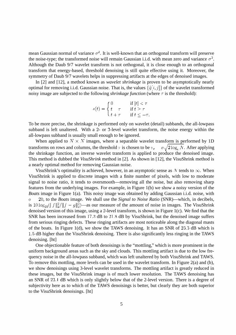
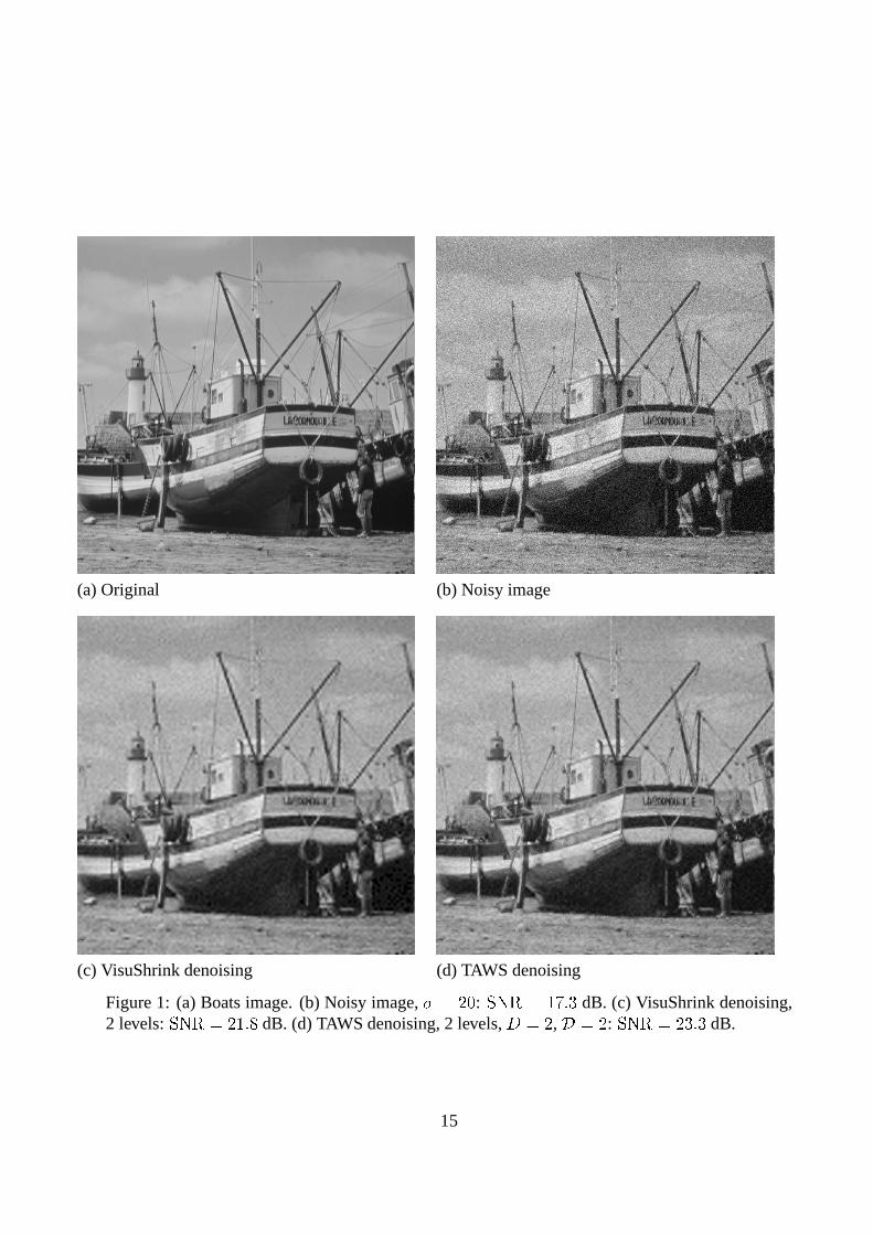
VisuShrink’s optimality is achieved, however, in an asymptotic sense as tends to � . WhenVisuShrink is applied to discrete images with a finite number of pixels, with low to moderatesignal to noise ratio, it tends to oversmooth—removing all the noise, but also removing sharpfeatures from the underlying images. For example, in Figure 1(b) we show a noisy version of theBoats image in Figure 1(a). This noisy image was obtained by adding Gaussian i.i.d. noise, with� � � > , to the Boats image. We shall use the Signal to Noise Ratio (SNR)—which, in decibels,is

� > ����+���� .�� � � ���� � � 2 ��� �� 0 —as our measure of the amount of noise in images. The VisuShrinkdenoised version of this image, using a � -level transform, is shown in Figure 1(c). We find that theSNR has been increased from

� �"! 9dB to � ��! < dB by VisuShrink, but the denoised image suffers

from serious ringing defects. These ringing artifacts are most noticeable along the diagonal mastsof the boats. In Figure 1(d), we show the TAWS denoising. It has an SNR of � 9#! 9 dB which is��! �

dB higher than the VisuShrink denoising. There is also significantly less ringing in the TAWSdenoising. [ht]

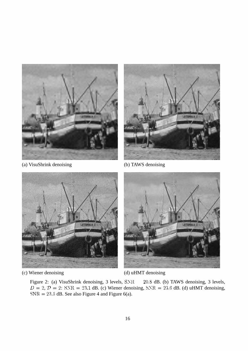
One objectionable feature of both denoisings is the “mottling,” which is more prominent in theuniform background areas such as the sky and clouds. This mottling artifact is due to the low fre-quency noise in the all-lowpass subband, which was left unaltered by both VisuShrink and TAWS.To remove this mottling, more levels can be used in the wavelet transform. In Figure 2(a) and (b),we show denoisings using 3-level wavelet transforms. The mottling artifact is greatly reduced inthese images, but the VisuShrink image is of much lower resolution. The TAWS denoising hasan SNR of � 9#! � dB which is only slightly below that of the 2-level version. There is a degree ofsubjectivity here as to which of the TAWS denoisings is better, but clearly they are both superiorto the VisuShrink denoisings. [ht]

5

The TAWS method is a combination of wavelet shrinkage with the predictive apparatus un-derlying Step 6 in the ASWDR method described above. This predictive apparatus makes use ofan assumed correlation between significant transform values at a threshold � and their children atthreshold � � � . In [13] it is shown that there is a high correlation between significant transform val-ues, whose magnitudes are at least � , and significant child transform values, whose magnitudes areat least � � � . Figure 4B in [13] provides a good illustration of this correlation. That figure shows aconditional histogram for fine scale horizontal subband transform values from the Boats test image.The conditional histogram is of ����+ � � � � (base 2 log of child magnitudes) versus ����+ � � � � (base 2log of parent magnitudes). It is clear from the figure that a large percentage of child magnitudesare above ����+ � � � � 2 �

, i.e., are either significant at the present threshold or will be significant atthe next threshold.

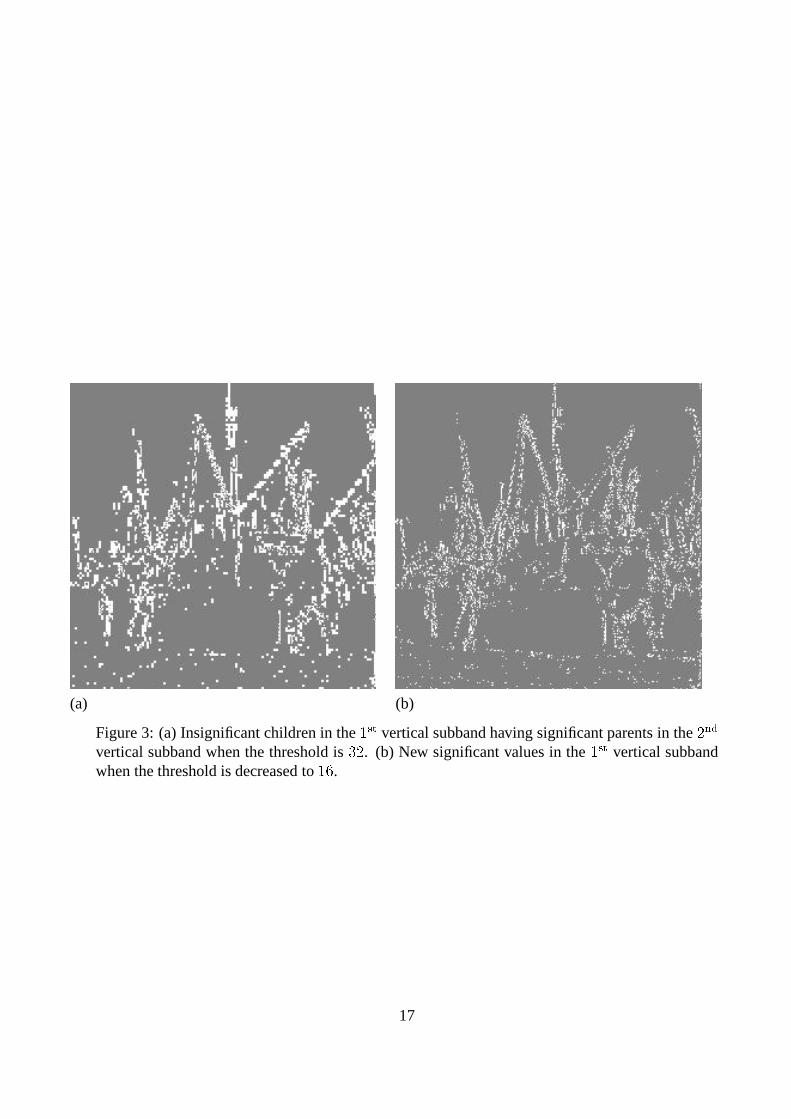
In Figure 3, we provide an illustration of this correlation. This figure was obtained from aDaub 9/7 wavelet transform of the Boats image. Figure 3(a) depicts the insignificant child values(shown in white) in the

�����level vertical subband of significant parent values in the ���� level

vertical subband, when the threshold is9 � . Figure 3(b) depicts the new significant values for the

half-threshold—those whose magnitudes are less than9 � and greater than or equal to

��—in the� ���

vertical subband. Notice that the child locations in Fig. 3(a) are good predictors for the newsignificant values in Fig. 3(b). Although these predictions are not perfectly accurate, there is agreat deal of overlap between the two images (in fact, the fraction of new significant values that liewithin the first part of the scan order created by Step 6 is

>#! � :). Notice also how the locations of

significant values are highly correlated with the location of edges in the Boats image. The scanningorder of ASWDR dynamically adapts to the locations of edge details in an image, and this enhancesthe resolution of these edges in ASWDR compressed images. By adapting this selection procedurefor significant values, the TAWS algorithm aims to improve resolution of edge details in denoising.As can be seen in Figures 1(d) and 2(b), this reduces ringing artifacts in the denoising of the noisyboat image. [ht]

A justification for these correlations for many natural noise-free images is based on the re-cursive nature of wavelet transforms; the parent values at any level being produced from a half-resolution version of the image that was used to produce the child transform values. When anorthogonal wavelet transform is applied to Gaussian i.i.d. random noise, however, the resultingtransform values are uncorrelated since they are also i.i.d. Gaussian random variables (with thesame variance as the untransformed noise). Therefore, noise transform values will exhibit par-ent/child correlations with a low probability. Although the Daub 9/7 wavelet transform is notorthogonal, it is close enough to an orthogonal transform that significant noise transform valuesstill exhibit low parent/child correlations.

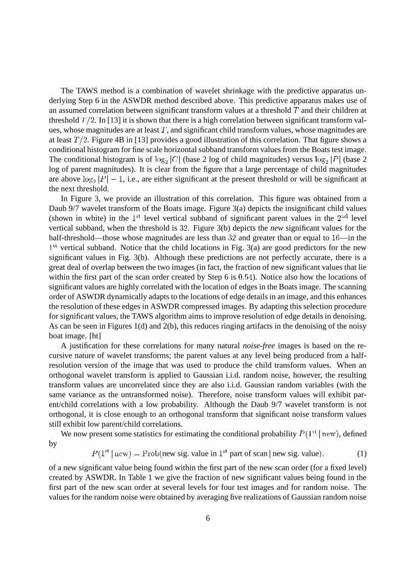
We now present some statistics for estimating the conditional probability � . � ��� � - ��� 0 , definedby

� . � ��� � - ��� 05����� ��� . new sig. value in� ���

part of scan � new sig. value0 �

(1)

of a new significant value being found within the first part of the new scan order (for a fixed level)created by ASWDR. In Table 1 we give the fraction of new significant values being found in thefirst part of the new scan order at several levels for four test images and for random noise. Thevalues for the random noise were obtained by averaging five realizations of Gaussian random noise

6

with mean 0 and standard deviation � < . (Although only five realizations were used, the results inTable 1 for the noise were quite stable showing deviations of no more than �

>#! >?�for all values.)

The data in this table clearly show that the probability in Eq. (1) is much greater for high-magnitudethreshold values for the test images than for the random noise. (By high-magnitude values we meanthose values whose magnitudes are greater than the standard deviation of the child subband.)

Parent level/Threshold 512 256 128 64 32 16 8Lena,

: ���, � � 9 �

(>#! 9�>

)>#! 9 � >#! : >#! � � >#! � >#! �< >#! �<

Goldhill,: ���

, � � 9�: . >#! >�>=0 >#! 9?� >#! : � >#! :=< >#! ��� >#! � >#! �<Boats,

: ���, � ��:�� . >#! � 9=0 >#! 9�9 >#! : � >#! � 9 >#! ?� >#! � >#! � :

Barbara,: ���

, � � 9�<(>#! >�

)>#! :=9 >#! � : >#! �> >#! �9 >#! �< >#! ���

Noise,: ���

, � � � � >#! >�> >#! > � >#! � � >#! � >#! ���Lena,

9�� � , � � � � . >#! > ��0 >#! 9?� >#! � > >#! � >#! � � >#! � >Goldhill,

9�� � , � ��� � . >#! >�:�0 >#! � : >#! 9 � >#! : � >#! � : >#! �Boats,

9�� � , � � � � . >#! >�>=0 . >#! � :�0 >#! :=> >#! :�� >#! � : >#! � >#! �Barbara,

9�� � , � � ��� >#! >?� >#! > � >#! � >#! 9�< >#! � � >#! �>Noise,

9�� � , � � � >#! >�> >#! >�9 >#! � >#! � < >#! ��<Lena, � �� , � � � � . >#! � � 0 >#! � � >#! � : >#! : � >#! 9�<

Goldhill, � �� , � �� . >#! > ��0 >#! 9 � >#! 9 � >#! :=> >#! : Boats, � �� , � � . >#! : �$0 >#! :=9 >#! � > >#! � � >#! � �

Barbara, � �� , � � � � >#! >�9 >#! � � >#! 9 � >#! � � >#! � �Noise, � �� , � � � : >#! >�> >#! >�9 >#! � � >#! ��� >#! � �

Table 1: Fraction of new significant values captured by first part of the new scan order created byASWDR. The standard deviations � are for the child subbands of each level. The Noise values wereobtained from averaging values for wavelet transforms of five realizations of Gaussian randomnoise with mean

>and standard deviation � < . A fraction in parentheses indicates that it may be an

unreliable estimate of the conditional probability � . ����� � - ��� 0 in Eq. (1), due to the number of newsignificant values being too small (less than � >�> ).

Notice that, for the random noise only, it is highly unlikely that a newly significant child valuewill be found in the first part of the scan order when the threshold is greater than the standarddeviation for the child subband. This facilitates the separation of noise dominated transform valuesfrom image dominated transform values at much lower thresholds than is possible with the standardwavelet thresholding methods.

These considerations lead to the following method of extending wavelet shrinkage so as toinclude more image dominated transform values lying below the VisuShrink threshold, 8 � . In theTAWS method, there are three parameters which are set at the start. One parameter is the descentindex � , which is a non-negative integer. The cutoff threshold 8 is then set at �78�� � �� , where theheight index � satisfies � � �

. For all of the TAWS denoisings reported on in this paper, the valueof this second parameter � was set as

� . In Figure 2(b), for example, the descent index is �� � ,

7

so 8 � ��8 � � : . Note that if �� >

and �� �

, then 8 � 8 � and TAWS reduces to the VisuShrinkmethod.

The third parameter is a depth index � , which is an integer lying between�

and � , where � isthe number of levels in the wavelet transform. We shall clarify below the nature of the depth index� .

The TAWS method consists of applying Steps 1 through 7 above, but with Step 6 modified asfollows. In this step the integer � is defined via the equation � � ��� �

� 8 � . That � is an integercan be arranged by a rescaling of wavelet transform values.

Step 6 (TAWS). For the first � cycles through Steps 4–6, produce a new scanning orderusing the Step 6 described above in the ASWDR method. For cycles �

�#�to �

�� , scan

only through children corresponding to significant parents in the highest subbands (levels 1to � ), while following the original recipe of Step 6 in the ASWDR algorithm for the other,lower, subbands.

From this description we can see that � must be no larger than � . For all of the TAWS denois-ings reported on below, it was found that setting � equal to the smaller of the values of � and �produced the best results.

Step 6 (TAWS) is phrased in terms of adapting a scanning order. Since a scanning order is a pro-cess of scanning through insignificant transform values in order to select those having magnitudeabove the present threshold, this provides a selection procedure for distinguishing transform valuesdominated by noise from those dominated by image. Unlike VisuShrink and cycle-spin threshold-ing, which use uniform thresholds for all transform values, the TAWS selection procedure usesdifferent thresholds ( � 8 � � � 8 � � � � ! ! ! � � 8 � � � ) which vary in their spatial locations, based on thepositions in the scan order of the transform values to which they are applied. Such a spatiallyadaptive thresholding gives TAWS a greater flexibility than a uniform thresholding method.

In the next section we shall demonstrate that the TAWS procedure outperforms VisuShrink,and is competitive with other, more state of the art, denoising methods.

3 Simulation results

In section 2 above, we gave one example of the performance of TAWS on denoising a noisy ver-sion of the Boats image. It performed significantly better than VisuShrink, both in terms of SNRand subjective visual quality. We shall now examine how TAWS performs on denoising the stan-dard test images—Lena, Goldhill, Boats, and Barbara—contaminated with additive i.i.d. Gaussiannoise of various standard deviations. We shall compare its performance on these test images withVisuShrink and with the following state of the art denoising methods: localized Wiener filtering[14], cycle-spin thresholding, and the uHMT methods.

In Table 2, we show a summary of how VisuShrink and TAWS performed in denoising thesetest images. In each case we list the highest SNR values for each method. For instance, for thefirst entry, the Lena image contaminated with noise of standard deviation

<, a 1-level transform

8

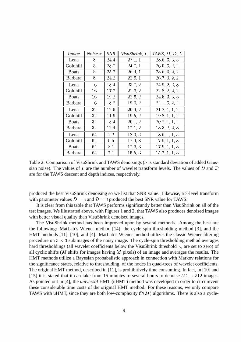
Image Noise � SNR VisuShrink, � TAWS, � , � , �Lena

< � :�! : � �"! � , � � <#! ,9,9,9

Goldhill< � 9#! � � :�! � ,

� � #! � , 9 , � , �Boats

< � � ! � � #! : ,� � <#! ,

9, � , �

Barbara< � :�! � ��� ! ,

� � #! � ,9, � , �

Lena�� � <#! : � 9#! � , � � :�! � , � , � ,

9Goldhill

�� � �"! � � ��! , � ��� ! < , � , � , �Boats

�� � � ! � ��� ! , � � :�! � , 9 ,9,9

Barbara�� � <#! � � � ! >

, � ��� ! � , 9 , � , �Lena

9 � � � ! � � >#! � , � � ��! � , � , � , �Goldhill

9 � ����! � � � ! �, � � � ! <

,�,�, �

Boats9 � � 9#! : � >#! � , � � >#! � ,

�,�, �

Barbara9 � � � ! : � �"! �

, � � <#! 9, � , � ,

9Lena

�: �"! � � <#! 9,9 � <#!

,�,�,9

Goldhill�: #! � � �"! :

,9 � �"! �

,�,�,9

Boats�: <#! � � �"!

,9 � �"! �

,�,�,9

Barbara�: �"! � � � ! �

,9 � � ! �

,�,�,9

Table 2: Comparison of VisuShrink and TAWS denoisings ( � is standard deviation of added Gaus-sian noise). The values of � are the number of wavelet transform levels. The values of � and �are for the TAWS descent and depth indices, respectively.

produced the best VisuShrink denoising so we list that SNR value. Likewise, a9-level transform

with parameter values �� 9

and �� 9

produced the best SNR value for TAWS.It is clear from this table that TAWS performs significantly better than VisuShrink on all of the

test images. We illustrated above, with Figures 1 and 2, that TAWS also produces denoised imageswith better visual quality than VisuShrink denoised images.

The VisuShrink method has been improved upon by several methods. Among the best arethe following: MatLab’s Wiener method [14], the cycle-spin thresholding method [3], and theHMT methods [11], [10], and [4]. MatLab’s Wiener method utilizes the classic Wiener filteringprocedure on

9 � 9subimages of the noisy image. The cycle-spin thresholding method averages

hard thresholdings (all wavelet coefficients below the VisuShrink threshold 8�� are set to zero) ofall cyclic shifts ( � shifts for images having � pixels) of an image and averages the results. TheHMT methods utilize a Bayesian probabalistic approach in connection with Markov relations forthe significance states, relative to thresholding, of the nodes in quad-trees of wavelet coefficients.The original HMT method, described in [11], is prohibitively time consuming. In fact, in [10] and[15] it is stated that it can take from 15 minutes to several hours to denoise

� � � � � � � images.As pointed out in [4], the universal HMT (uHMT) method was developed in order to circumventthese considerable time costs of the original HMT method. For these reasons, we only compareTAWS with uHMT, since they are both low-complexity � . � 0

algorithms. There is also a cycle-

9

spin averaged version of uHMT which averages uHMT denoisings of all cyclic shifts of the noisyimage. We shall refer to this method as uHMT-spin.

As with cycle-spin thresholding and uHMT-spin, there is a cycle-spin averaged version ofTAWS, which we shall refer to as TAWS-spin. The TAWS-spin method simply consists of aver-aging TAWS denoisings of a finite number of cyclic shifts of the image:

����� �52 ���� 2 % �for��� % � >

, ��,! ! !

, . In Table 3 we list the results for � � , which is an averaging of TAWSdenoisings of � � different shiftings, under the heading T-S. Experiments show that for

�-, � -, or9

-level transforms, the SNR values rapidly converge as the number of shifts increases, and that � � yields a good compromise between increased SNR values and increased time and memoryconsumption needed to perform averages. It is important to remember that although cycle-spinmethods are � . � ����+�� 0

methods, it still requires considerable memory resources to store partsof previously computed transforms of shifted images. The TAWS-spin method requires only amodest increase in memory resources, just two extra arrays equal in size to the image array forholding the image shifts and for storing partial averages.

Image, � SNR VS W HMT TAWS C-S H-S T-SLena,

< � :�! : � �"! � 28.9 28.9 � <#! � <#! � 29.9 � � ! �Goldhill,

< � 9#! � � :�! � � #! � � #! > 26.5 � #! 9 � #! � 27.0Boats,

< � � ! � � #! : � <#! � � <#! : 28.6 � <#! : 29.3 29.3Barbara,

< � :�! � ��� ! � :�! � � 9#! : 26.7 � 9#! � � :�! � 27.0Lena,

�� � <#! : � 9#! � � � ! > 25.5 � :�! � � � ! � 26.4 � #! �Goldhill,

�� � �"! � � ��! 23.3 ��� ! < ��� ! < � 9#! � � 9#! � 23.6Boats,

�� � � ! � ��� ! 25.0 � :�! � :�! � � � ! > � � ! 9 25.5Barbara,

�� � <#! � � � ! >22.1 � >#! > 22.1 ��� ! > � >#! � 22.5

Lena,9 � � � ! � � >#! � � � ! �

22.3 � ��! � ��� ! � 22.9 ��� ! �Goldhill,

9 � ����! � � � ! � � <#! 20.2

� � ! < � >#! � 20.8 � >#! :Boats,

9 � � 9#! : � >#! � � >#! � 21.4 � >#! � � ��! < 21.9 � ��! Barbara,

9 � � � ! : � �"! � � <#! � � �"! �18.3

� <#! � � <#! �18.6

Lena,�: �"! � � <#! 9 � :�! �

19.2� <#! � <#! <

19.6� � ! 9

Goldhill,�: #! � 9 � �"! : � 9#!

17.7� �"! � � �"! �

18.1� <#! >

Boats,�: <#! � � �"! � � ! �

18.6� �"! � � <#! 9

18.9� <#! �

Barbara,�: �"! � � � ! � � 9#!

16.0� � ! � � � ! �

16.2 16.2

Table 3: Comparison of various denoisings ( � is standard deviation of added Gaussian noise).Key: VS is VisuShrink, W is MatLab’s Wiener method, HMT is the uHMT method, TAWS is theTAWS method, C-S is the cycle-spin thresholding method, H-S is the uHMT-spin method, and T-Sis the TAWS-spin method.

In columns 3–6 of Table 3, we list the SNR values for denoising the same test images as inTable 2 for each of the methods—VisuShrink, MatLab’s Wiener, uHMT, and TAWS—which donot make use of cycle-spin averaging. In columns 7–9, we list the SNR values for the methods—

10

cycle-spin, uHMT-spin, and TAWS-spin—which do utilize cycle-spin averaging. For the fournon-averaged methods, the largest SNR value for each of the four tested methods is displayed inbold-face. Likewise, the largest SNR value for each of the three cycle-spin averaged methods isdisplayed in bold-face. We first discuss the non-averaged methods, and then treat the cycle-spinaveraged methods. In every case, the TAWS method employs the same values for � , � , and � , aswere used in the denoisings summarized in Table 2. The cycle-spin thresholding method uses foreach image the value of � used for the VisuShrink denoisings in Table 2. We shall explain belowwhich values of � , � , and � were used in the TAWS-spin denoisings.

For the non-averaged methods, the data in Table 3 show that no one method is superior amongthe three best (Wiener, uHMT, and TAWS). Wiener and TAWS yield higher SNR values for low ormoderate noise levels. On the other hand, uHMT performs better with higher noise levels, muchbetter than Wiener and moderately better than TAWS. Note that TAWS and Wiener significantlyoutperform uHMT on the Barbara denoisings. The reason for this is that uHMT is based on asingle set of prior assumptions for the image data. More precisely, uHMT assumes a particular rateof decay of wavelet coefficients across scales. The default choice of this decay rate, specified inthe MatLab code in [15] and derived in [10], is appropriate for smoother images (images with verylittle energy in higher spatial frequencies) like Lena. It is not appropriate for an image like Barbarawhich has much greater energy in higher spatial frequencies. This explains why uHMT performsso well on denoising the Lena images, but not so well on the Barbara images.

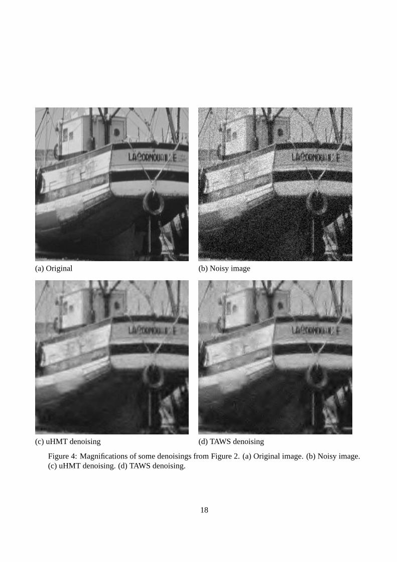
Since SNR values are not precisely equivalent to human perception, it is important to exam-ine some denoised images using these methods. We show in Figure 2, the Wiener and uHMTdenoisings of the noisy image from Figure 1(b), as well as the VisuShrink and TAWS denoisingsdiscussed above. Although the Wiener denoising has the highest SNR, it also exhibits a largeamount of residual, low frequency noise, which makes it perceptually inferior to both the TAWSand uHMT denoisings. This is even more clearly revealed by comparing the magnification of theWiener denoised image, in Figure 6(a), with the magnifications of the uHMT and TAWS denois-ings, in Figure Figures 4(c) and (d). Comparing the TAWS and uHMT denoisings in Figure 2, theTAWS denoising appears sharper, more focused, although it retains some residual noise.

This last point is more clearly shown in the magnifications in Figure 4. The TAWS denoisingin Figure 4(d) has a sharper, more focused, appearance. In contrast, the uHMT denoising in Figure4(c) appears slightly blurred, slightly out of focus. On the other hand, there are isolated noisy spotsretained in the TAWS image, while the uHMT image appears completely free of random noise. [ht]

This raises an interesting question for future research. Since the residual noise retained inthe TAWS denoisings consists of isolated noisy spots, it is possible that a filtering out of isolatedtransform values in the highest subbands could be used to post-process the TAWS denoised images.Preliminary results show this to be effective. It also appears to be of considerable value in denoisingimages contaminated with speckle noise. Details will be reported in a subsequent paper.

Another possibility is to utilize decay rate assumptions, as uHMT does, in order to remove somewavelet coefficients which survive the correlation filter used by TAWS. Since these coefficients arethe source of the isolated noise spots, their removal would eliminate these noise spots.

A third option is to change the value of the height index � . We show below that this optionworked well for improving TAWS-spin denoisings.

11

We now turn to simulation results for the spin-averaged methods. The SNR values for our testimages are shown in the last three columns of Table 3. The TAWS-spin denoisings used the value�� � , and the values of �

� �, � , and � , from those shown in Table 2. For example, the noisy

Lena image with � � <, was denoised by TAWS-spin using �

� � , �� :

, �� 9

, and �� 9

(while the TAWS denoising used �� � , � � 9

, �� 9

, and �� 9

).These results are reminiscent of the ones just discussed for the non-averaged methods. Again,

there is no method which is clearly superior for all noise levels.In Figure 5, we show denoised images of the noisy boat image from Figure 1(a). In addition to

the TAWS-spin denoising using �� � , we have also shown a TAWS-spin denoising with �

� �(which is the value of � used for TAWS denoisings). The SNR value for TAWS-spin with �

� �is

>#! :dB larger than when �

� � is used. Furthermore, although it is hard to see, there isconsiderably less residual noise in the TAWS-spin denoising for �

� � . By using a higher value of� , and a higher value of � , the TAWS-spin denoisings are applying the Step 6 (TAWS) selectionprocedure over a greater range of threshold values (beginning with a higher value of � 8 � ) and isthus able to select out more residual noise values than TAWS alone can do. For the simulationsreported in Table 3, we found that using �

� � in place of �� � generally produced higher

SNR values and very little residual noise in TAWS-spin denoised images. At this time, we havenot been able to discover a similar value of � which works as well for TAWS denoisings ( �

� �reduces residual noise, but also significantly lowers SNR values). [ht]

In Figure 6, we show magnifications of some denoisings of the noisy boat image from Figure1. The MatLab Wiener denoising is clearly inferior to both the TAWS-spin and the uHMT-spindenoising. The TAWS-spin image is the sharpest, most clearly focused, of the denoisings. Inaddition, it exhibits essentially no residual noise. The uHMT-spin image also seems to containno residual noise, but is slightly more blurred than the TAWS-spin and the cycle-spin thresholddenoisings. [ht]

4 Conclusion

We have described two new methods for denoising images, the TAWS method and the TAWS-spinmethod, which provide denoisings comparable to state of the art methods. A problem for futureresearch is how to choose the parameters � and � used in the TAWS and TAWS-spin method(and how to choose the parameter � in the TAWS method). One possibility is an initial analysis ofthe statistical trends at higher thresholds (several standard deviations above the noise), in order topredict a good ending threshold. Better predictive schemes than the parent-child scheme employedat present should also be investigated, as they will reduce the number of isolated, residual, noisespots that appear in TAWS denoisings (as well as increase the SNR). For example, use might bemade of a lack of clustering [11] in higher spatial frequency subbands (this is the basis for theisolation filter described above in section 3). Finally, integration of TAWS with ASWDR into acombination compressor/denoiser is an important goal for future research.

12

Acknowledgements

The first author would like to thank the University of Wisconsin for its generous support, and theBoston University Departments of Mathematics and of Electrical & Computer Engineering fortheir hospitality, during his 1998–99 sabbatical year when the initial version of this paper waswritten. He also wishes to thank Truong Q. Nguyen for his help and encouragement.

References

[1] J.S. Walker. A lossy image codec based on adaptively scanned wavelet difference reduc-tion. To appear in Optical Engineering.

[2] D. Donoho and I. Johnstone. Ideal spatial adaptation via wavelet shrinkage. Biometrika,Vol. 81, pp. 425–455, Dec. 1994.

[3] R. Coifman and D. Donoho, Translation-invariant denoising. In Wavelets and Statistics,Lecture Notes in Statistics, Springer, 1995.

[4] J.K. Romberg, H. Choi, and R.G. Baraniuk, Shift-invariant denoising using wavelet-domain hidden Markov trees. Proc.

9�9 � � Asilomar Conference, Pacific Grove, CA, October1999.

[5] A. Cohen, I. Daubechies, and J.-C. Feauveau. Biorthogonal bases of compactly supportedwavelets. Commun. on Pure and Appl. Math., Vol. 45, pp. 485-560, 1992.

[6] J.M. Shapiro. Embedded image coding using zerotrees of wavelet coefficients. IEEE Trans.Signal Proc., Vol. 41, No. 12, pp. 3445–3462, Dec. 1993.

[7] A. Said and W.A. Pearlman. A new, fast, and efficient image codec based on set partitioningin hierarchical trees. IEEE Trans. on Circuits and Systems for Video Technology, Vol. 6,No. 3, pp. 243–250, June 1996.

[8] S. Servetto, J.R. Rosenblatt, and K. Ramchandran, A binary Markov model for the quan-tized wavelet coefficients of images and its rate/distortion optimization. Proc. of ICIP1997, Vol. 3, pp. 82–85.

[9] S. G. Chang, B. Yu, and M. Vetterli, Image denoising via lossy compression and waveletthresholding. Proc. of ICIP 1997, Vol. 1, pp. 604–607.

[10] J.K. Romberg, H. Choi, and R.G. Baraniuk, Bayesian tree-structured image modeling us-ing wavelet-domain hidden Markov models. Proc. SPIE Technical Conference on Math-ematical Modeling, Bayesian Estimation, and Inverse Problems, pp. 31–44, Denver, July1999.

13

[11] M.S. Crouse, R.D. Nowak, and R.G. Baraniuk, Wavelet-based statistical signal processingusing hidden Markov models. IEEE Trans. Signal Proc., Vol. 46, No. 4, pp. 886–902, April1998.

[12] D. Donoho, I. Johnstone, G. Kerkyacharian, and D. Picard. Wavelet shrinkage: asymp-topia? J. Royal Stat. Soc. B, Vol. 57, No. 2, pp. 301–369, 1995.

[13] R.W. Buccigrossi and E.P. Simoncelli, Image compression via joint statistical characteri-zation in the wavelet domain. IEEE Trans. on Image Proc., Vol. 8, No. 12, pp. 1688–1701,1999.

[14] MatLab, a product of The Math Works, Inc. The localized Wiener method is calledwiener2 in MatLab, and is part of MatLab’s Image Processing Toolbox.

[15] J.K. Romberg, H. Choi, and R.G. Baraniuk, MatLab code for Hidden Markov denoising,located at the URL:

http://www-dsp.rice.edu/software/WHMT/

14

(a) Original (b) Noisy image

(c) VisuShrink denoising (d) TAWS denoising

Figure 1: (a) Boats image. (b) Noisy image, � � � > : ������ � �"! 9

dB. (c) VisuShrink denoising,2 levels: �����

� � ��! < dB. (d) TAWS denoising, 2 levels, �� � , � � � : ����� � � 9#! 9 dB.

15

(a) VisuShrink denoising (b) TAWS denoising

(c) Wiener denoising (d) uHMT denoising

Figure 2: (a) VisuShrink denoising, 3 levels, ������ � >#! < dB. (b) TAWS denoising, 3 levels,

�� � , � � � : ����� � � 9#! � dB. (c) Wiener denoising, �����

� � 9#! dB. (d) uHMT denoising,�����

� � 9#! � dB. See also Figure 4 and Figure 6(a).

16

(a) (b)

Figure 3: (a) Insignificant children in the�����

vertical subband having significant parents in the � ��vertical subband when the threshold is

9 � . (b) New significant values in the� ���

vertical subbandwhen the threshold is decreased to

��.

17

(a) Original (b) Noisy image

(c) uHMT denoising (d) TAWS denoising

Figure 4: Magnifications of some denoisings from Figure 2. (a) Original image. (b) Noisy image.(c) uHMT denoising. (d) TAWS denoising.

18

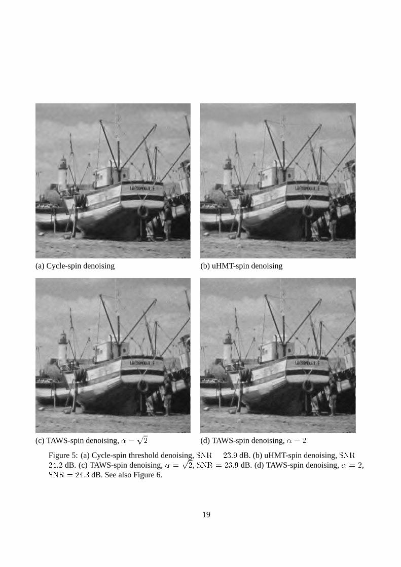
(a) Cycle-spin denoising (b) uHMT-spin denoising

(c) TAWS-spin denoising, �� � (d) TAWS-spin denoising, �

� �Figure 5: (a) Cycle-spin threshold denoising, �����

� � 9#! � dB. (b) uHMT-spin denoising, ������

� :�! � dB. (c) TAWS-spin denoising, �� � , ����� � � 9#! � dB. (d) TAWS-spin denoising, �

� � ,�����

� � :�! 9 dB. See also Figure 6.

19

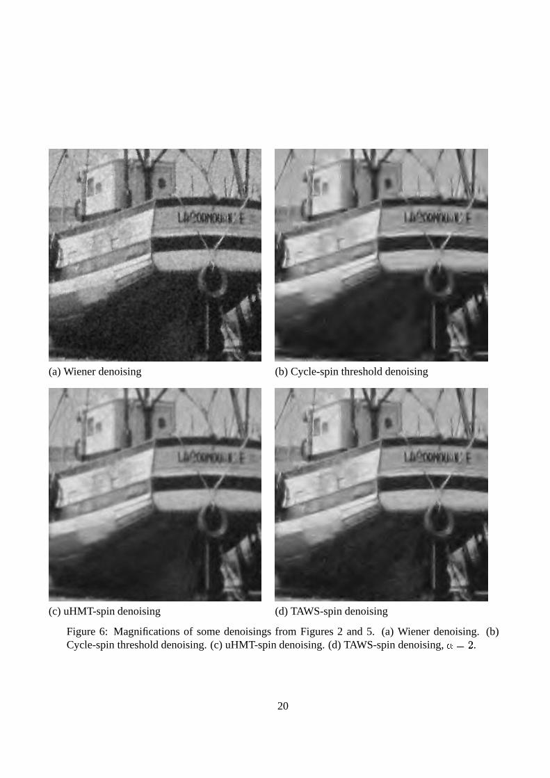
(a) Wiener denoising (b) Cycle-spin threshold denoising

(c) uHMT-spin denoising (d) TAWS-spin denoising

Figure 6: Magnifications of some denoisings from Figures 2 and 5. (a) Wiener denoising. (b)Cycle-spin threshold denoising. (c) uHMT-spin denoising. (d) TAWS-spin denoising, �

� � .

20