image processing with python - uni-hamburg.deseppke/...visualization with matplotlib and the spyder...
TRANSCRIPT

Image Processing with Python
An introduction to the use of Python, NumPy, SciPy and matplotlib
for image processing tasks
In preparation for the exercises of the Master course module Image Processing 1
at winter semester 2013/14
Benjamin Seppke ([email protected]) 17.10.2013

Outline Introduction
Presenting the Python programming language
Image processing with NumPy and SciPy
Visualization with matplotlib and the spyder IDE
Summary

Outline Introduction
Presenting the Python programming language
Image processing with NumPy and SciPy
Visualization with matplotlib and the spyder IDE
Summary

Prerequisites (Software) Python (we use version 2.X with X>5)
http://www.python.org
NumPy and SciPy (with PIL: http://www.pythonware.com/products/pil ) http://www.scipy.org
matplotlib http://matplotlib.org
spyder IDE http://code.google.com/p/spyderlib

Installing Python and packages
Linux All of the prerequisites should be installable by means of the
package manager of the distribution of your choice.
Mac OS X Install the MacPorts package manager (http://www.macports.org)
and use this to get all necessary packages.
Windows Python-(x,y) (http://code.google.com/p/pythonxy) contains all
necessary packages in binary form and an installer.

Goals for today... Draw interest to another programming language,
namely: Python
Motivation of an interactive Workflow („Spielwiese“)
„Easy access” into practical image processing tasks using NumPy, SciPy, matplotlib and spyder
Finally: Give you the ability to solve the exercises of this course

Outline Introduction
Presenting the Python programming language
Image processing with NumPy and SciPy
Visualization with matplotlib and the spyder IDE
Summary

Introducing Python
The following introduction is based on the official „Python-Tutorial“
http://docs.python.org/tutorial/index.html

Python „Python is an easy to learn, powerful programming language. [...]
Python’s elegant syntax and dynamic typing, together with its interpreted nature, make it an ideal language for scripting and rapid application development in many areas on most platforms.“
„By the way, the language is named after the BBC show “Monty Python’s Flying Circus” and has nothing to do with reptiles.“
The Python Tutorial, Sep. 2010

Why another language? Why Python?
Interactive: no code/compile/test-cycle!
A lot of currently needed and easy accessible functionality compared with traditional scripting languages!
Platform independent and freely available!
Large user base and good documentation!
Forces compactness and readability of programs by syntax!
Some say: can be learned in 10 minutes...

Getting in touch with Python (2.X)
All of this tutorial will use the interactive mode: Start the interpreter: python Or, an advanced interpreter: ipython
1. Example: > python
Python 2.7 (#1, Feb 28 2010, 00:02:06)
Type "help", "copyright", "credits" or "license" for more information.
>>> the_world_is_flat = True
>>> if the_world_is_flat:
... print "Be careful not to fall off!"
...
Be careful not to fall off!
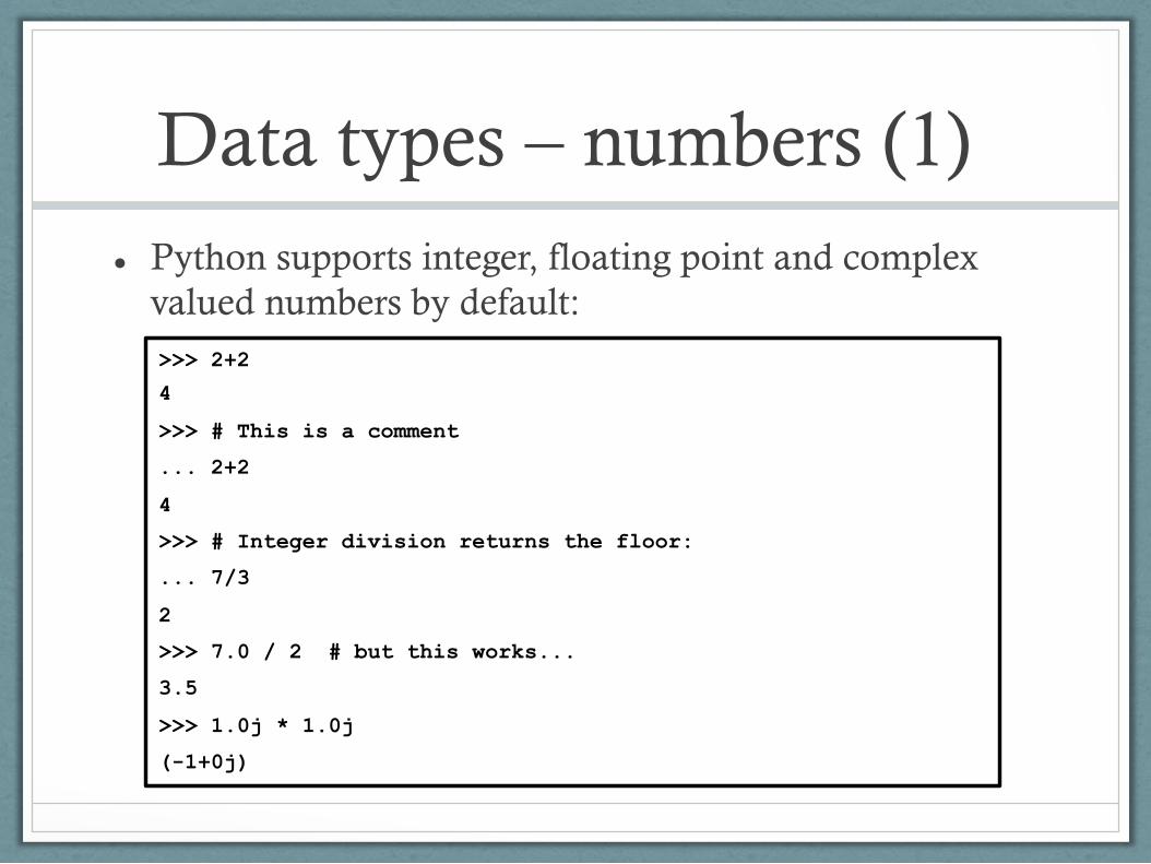
Data types – numbers (1) Python supports integer, floating point and complex
valued numbers by default: >>> 2+2
4
>>> # This is a comment
... 2+2
4
>>> # Integer division returns the floor:
... 7/3
2
>>> 7.0 / 2 # but this works...
3.5
>>> 1.0j * 1.0j
(-1+0j)

Data types – numbers (2) Assignments and conversions:
>>> a=3.0+4.0j
>>> float(a)
Traceback (most recent call last):
File "<stdin>", line 1, in ?
TypeError: can't convert complex to float; use abs(z)
>>> a.real
3.0
>>> a.imag
4.0
>>> abs(a) # sqrt(a.real**2 + a.imag**2)
5.0

Special variables Example: last result „_“ (only in interactive mode):
Many more in ipython!
>>> tax = 12.5 / 100
>>> price = 100.50
>>> price * tax
12.5625
>>> price + _
113.0625
>>> round(_, 2)
113.06

Data types – strings Sequences of chars (like e.g. in C), but immutable!
>>> word = 'Help' + 'A'
>>> word
'HelpA'
>>> '<' + word*5 + '>'
'<HelpAHelpAHelpAHelpAHelpA>'
>>> 'str' 'ing' # <- This is ok
'string'
>>> word[4]
'A'
>>> word[0:2]
'He'
>>> word[2:] # Everything except the first two characters
'lpA'
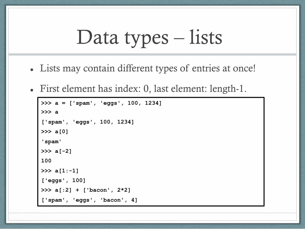
Data types – lists Lists may contain different types of entries at once!
First element has index: 0, last element: length-1. >>> a = ['spam', 'eggs', 100, 1234]
>>> a
['spam', 'eggs', 100, 1234]
>>> a[0]
'spam'
>>> a[-2]
100
>>> a[1:-1]
['eggs', 100]
>>> a[:2] + ['bacon', 2*2]
['spam', 'eggs', 'bacon', 4]

The first program (1) Counting Fibonacci series
>>> # Fibonacci series:
... # the sum of two elements defines the next
... a, b = 0, 1
>>> while b < 10:
... print b
... a, b = b, a+b
...
1
1
2
3
5
8
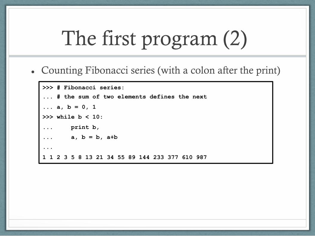
The first program (2) Counting Fibonacci series (with a colon after the print)
>>> # Fibonacci series:
... # the sum of two elements defines the next
... a, b = 0, 1
>>> while b < 10:
... print b,
... a, b = b, a+b
...
1 1 2 3 5 8 13 21 34 55 89 144 233 377 610 987

Conditionals – if Divide cases in if/then/else manner:
>>> x = int(raw_input("Please enter an integer: "))
Please enter an integer: 42
>>> if x < 0:
... x = 0
... print 'Negative changed to zero'
... elif x == 0:
... print 'Zero'
... elif x == 1:
... print 'Single'
... else:
... print 'More'
...
More

Control flow – for (1) Python‘s for-loop:
is indeed a for-each-loop!
>>> # Measure the length of some strings:
... a = ['two', 'three', 'four']
>>> for x in a:
... print x, len(x)
...
two 3
three 5
four 4
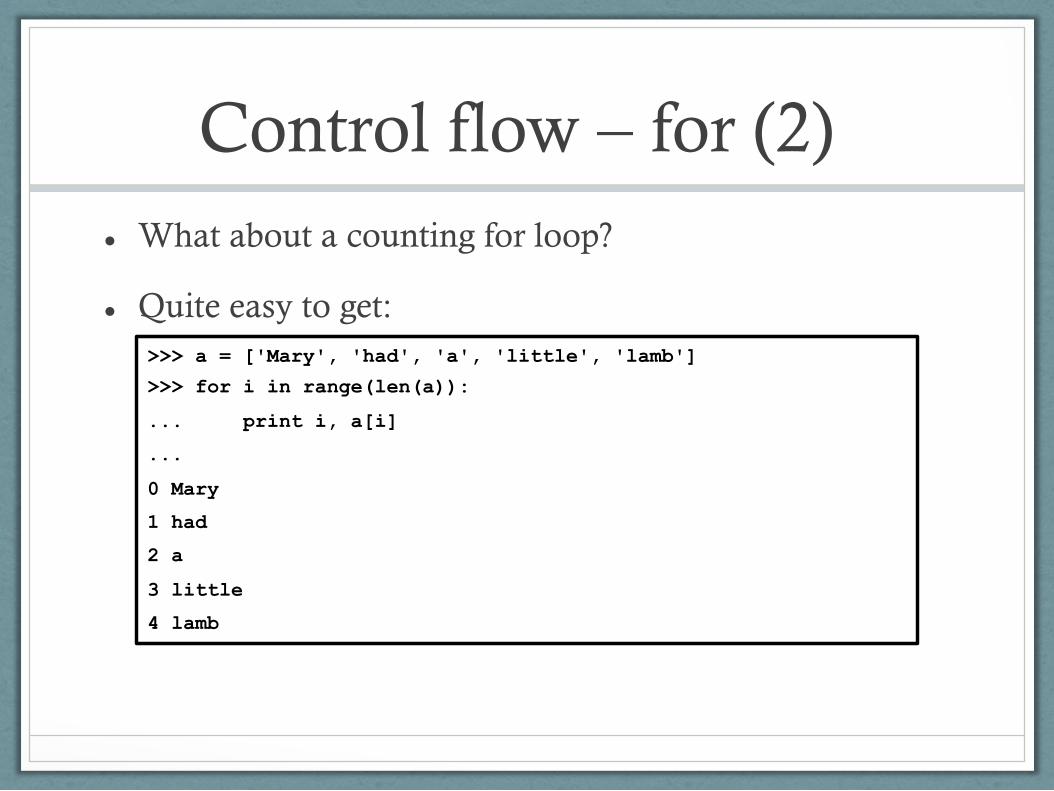
Control flow – for (2) What about a counting for loop?
Quite easy to get: >>> a = ['Mary', 'had', 'a', 'little', 'lamb']
>>> for i in range(len(a)):
... print i, a[i]
...
0 Mary
1 had
2 a
3 little
4 lamb

Defining functions (1) Functions are one of the most important way to
abstract from problems and to design programs: >>> def fib(n): # write Fibonacci series up to n
... """Print a Fibonacci series up to n."""
... a, b = 0, 1
... while a < n:
... print a,
... a, b = b, a+b
...
>>> # Now call the function we just defined:
... fib(2000)
0 1 1 2 3 5 8 13 21 34 55 89 144 233 377 610 987 1597
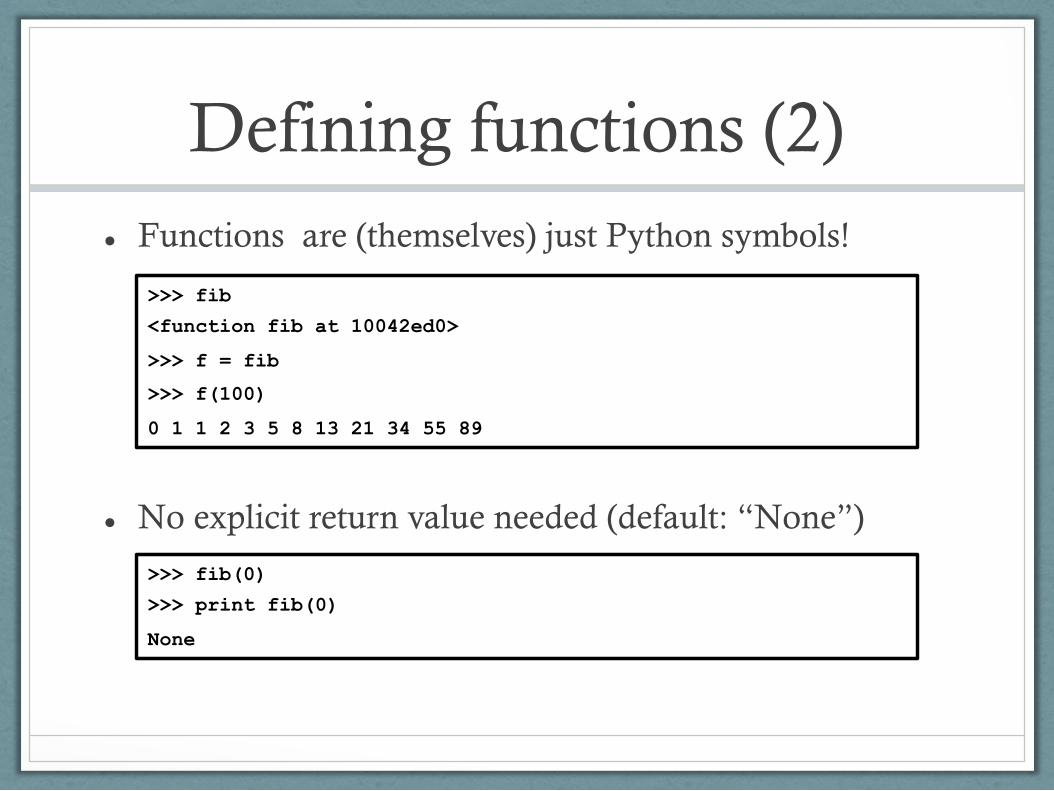
Defining functions (2) Functions are (themselves) just Python symbols!
No explicit return value needed (default: “None”)
>>> fib
<function fib at 10042ed0>
>>> f = fib
>>> f(100)
0 1 1 2 3 5 8 13 21 34 55 89
>>> fib(0)
>>> print fib(0)
None

Defining functions (3) Fibonacci series with a list of numbers as return value:
>>> def fib2(n): # return Fibonacci series up to n
... """Return a list containing the Fibonacci series up to n."""
... result = []
... a, b = 0, 1
... while a < n:
... result.append(a) # see below
... a, b = b, a+b
... return result
...
>>> f100 = fib2(100) # call it
>>> f100 # write the result
[0, 1, 1, 2, 3, 5, 8, 13, 21, 34, 55, 89]

Function argument definitions (1)
Named default arguments:
def ask_ok(prompt, retries=4, complaint='Yes or no, please!'):
while True:
ok = raw_input(prompt)
if ok in ('y', 'ye', 'yes'):
return True
if ok in ('n', 'no', 'nop', 'nope'):
return False
retries = retries - 1
if retries < 0:
raise IOError('refuse user')
print complaint
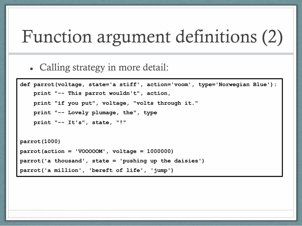
Function argument definitions (2)
Calling strategy in more detail:
def parrot(voltage, state='a stiff', action='voom', type='Norwegian Blue'):
print "-- This parrot wouldn't", action,
print "if you put", voltage, "volts through it."
print "-- Lovely plumage, the", type
print "-- It's", state, "!"
parrot(1000)
parrot(action = 'VOOOOOM', voltage = 1000000)
parrot('a thousand', state = 'pushing up the daisies')
parrot('a million', 'bereft of life', 'jump')

Excurse: lambda abstraction If you want, you can go functional with Python, e.g.
using the provided lambda abstractor: >>> f = lambda x, y: x**2 + 2*x*y + y**2
>>> f(1,5)
36
>>> (lambda x: x*2)(3)
6

Modules If you have saved this as „fibo.py“:
…you have already written your first Python module. Call it using:
# Fibonacci numbers module
def fib(n): # return Fibonacci series up to n
result = []
a, b = 0, 1
while b < n:
result.append(b)
a, b = b, a+b
return result
>>> import fibo
>>> fibo.fib(100)
[1, 1, 2, 3, 5, 8, 13, 21, 34, 55, 89]

Summary of Python You‘ll learn Python the best:
… by means of practical use of the language! … especially not by listening to lectures!
Python has a lot more to offer! E.g.: A class system, error handling, IO, GUI, Networking
The slides shown before should have shown that: Getting in touch is quite easy!
The learning rate is comparably steep!
You get early and valuable experiences of achievements!
All this makes Python so popular!!

Outline Introduction
Presenting the Python programming language
Image processing with NumPy and SciPy
Visualization with matplotlib and the spyder IDE
Summary

Image processing with NumPy and SciPy
Unfortunately, it is not possible to give a complete introduction in either NumPy or SciPy.
The image processing introduction is based on: http://scipy-lectures.github.io/advanced/image_processing
More material regarding NumPy can e.g. be found at: http://numpy.scipy.org
A good beginner‘s tutorial is provided at: http://www.scipy.org/Tentative_NumPy_Tutorial

Images as efficient arrays?! In many programming environments, like e.g. MatLab,
images are represented as random access arrays
However, Python‘s built-in array is often neither flexible nor powerful enough for image processing
Thus: use NumPy arrays for image representation.
Idea of a first (very basic) workflow: Load images using scipy.misc (via PIL)
Process the images using NumPy and Scipy
Save the images using scipy.misc (via PIL)
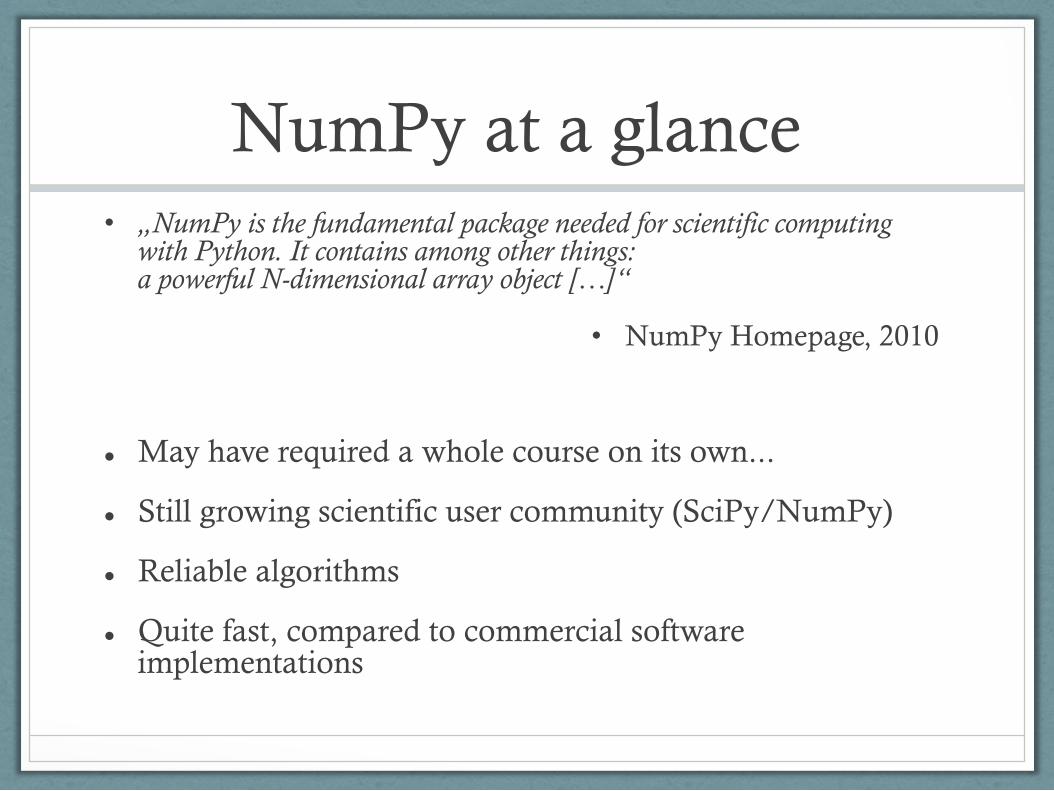
NumPy at a glance • „NumPy is the fundamental package needed for scientific computing
with Python. It contains among other things: a powerful N-dimensional array object […]“
• NumPy Homepage, 2010
May have required a whole course on its own...
Still growing scientific user community (SciPy/NumPy)
Reliable algorithms
Quite fast, compared to commercial software implementations

Loading and saving images Load an image into a NumPy array (requires PIL)
Saving a NumPy array as an image (requires PIL)
Attention: Usually only 2d- and 3d-arrays with datatype„uint8“ (0 – 255) can be saved as images. A type conversion may be necessary before saving!
>>> import numpy as np
>>> from scipy import misc
>>> img = misc.imread('lena.png‘)
...
>>> img = misc.imread('lena.png‘)
>>> misc.imsave('lena_copy.png‘, img)

„Hello Image“ First example: Load, “view” and save an image:
...
>>> img = misc.imread('lena.png‘) #or: img = misc.lena()
>>> img
array([[162, 162, 162, ..., 170, 155, 128],
...,
[ 44, 44, 55, ..., 104, 105, 108]])
>>> misc.imsave(img, 'lena_copy.png‘)

NumPy image representation (1)
Gray-value images: ...
>>> img
array([[162, 162, 162, ..., 170, 155, 128],
[162, 162, 162, ..., 170, 155, 128],
[162, 162, 162, ..., 170, 155, 128],
...,
[ 43, 43, 50, ..., 104, 100, 98],
[ 44, 44, 55, ..., 104, 105, 108],
[ 44, 44, 55, ..., 104, 105, 108]])

NumPy image representation (2)
RGB-value images: ...
>>> img_rgb
array([[[121, 112, 131], ..., [139, 144, 90]], [[ 89, 82, 100], ..., [146, 153, 99]],
[[ 73, 66, 84], ..., [144, 153, 98]],
...,
[[ 87, 106, 76], ..., [119, 158, 95]],
[[ 85, 101, 72], ..., [120, 156, 94]],
[[ 85, 101, 74], ..., [118, 154, 92]]], dtype=uint8)

NumPy slicing and index tricks
Extract channels using slicing
Extract sub-images using index ranges:
Attention: NumPy often creates views and does not copy your data, when using index tricks! Compare to Call-By-Reference Semantics
>>> img_rgb[:,:,0] # <-- red channel >>> img_rgb[...,0] # same as above, fix inner-most dim. to 0 >>> img_rgb[...,1] # <-- green channel >>> img_rgb[...,2] # <-- blue channel >>> img_rgb[...,-1] # same as above, since blue is the last ch.
>>> img_rgb[100:200,100:200,0] # <-- red channel, size 100x100 px >>> img[100:200,100:200] # <-- 100x100 px of gray-scale image

Basic Image Processing (1) Example: Invert an image (create the negative):
... >>> img_invert = 255 - img
>>> img_rgb_invert = 255 – img_rgb # <-- works for rgb too!

Basic Image Processing (2) Example: Threshold an image:
... >>> threshold = 100 >>> mask = img < threshold
>>> masked_img = img.copy()
>>> masked_img[mask] = 0
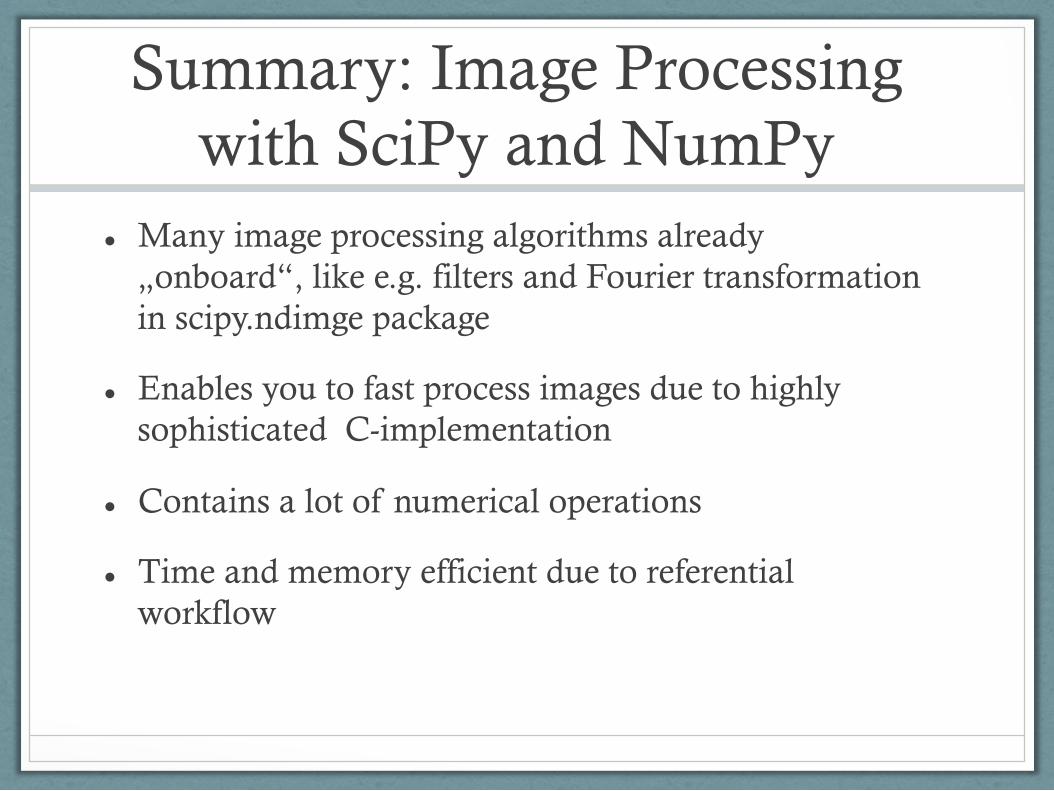
Summary: Image Processing with SciPy and NumPy
Many image processing algorithms already „onboard“, like e.g. filters and Fourier transformation in scipy.ndimge package
Enables you to fast process images due to highly sophisticated C-implementation
Contains a lot of numerical operations
Time and memory efficient due to referential workflow

Outline Introduction
Presenting the Python programming language
Image processing with NumPy and SciPy
Visualization with matplotlib and the spyder IDE
Summary

Visualization with matplotlib
“matplotlib is a python 2D plotting library which produces publication quality figures in a variety of hardcopy formats and interactive environments across platforms. matplotlib can be used in python scripts, the python and ipython shell...“
http://matplotlib.org, October 2013
This introduction is based on the matplotlib image tutorial: http://matplotlib.org/users/image_tutorial.html

Showing images interactively
• Use matplotlib to show an image figure: >>> import matplotlib.pyplot as plt >>> from scipy import misc >>> img = misc.imread(‚stinkbug.png‘) # <-- stored as a gray rgb image >>> lum_img = img[...,0] >>> img_plot = plt.imshow(img) >>> img_plot.show() >>> img_lum_plot = plt.imshow(lum_img) >>> img_lum_plot.show() >>> img_lum_plot.set_cmap(gray) # also try hot, spectral etc.
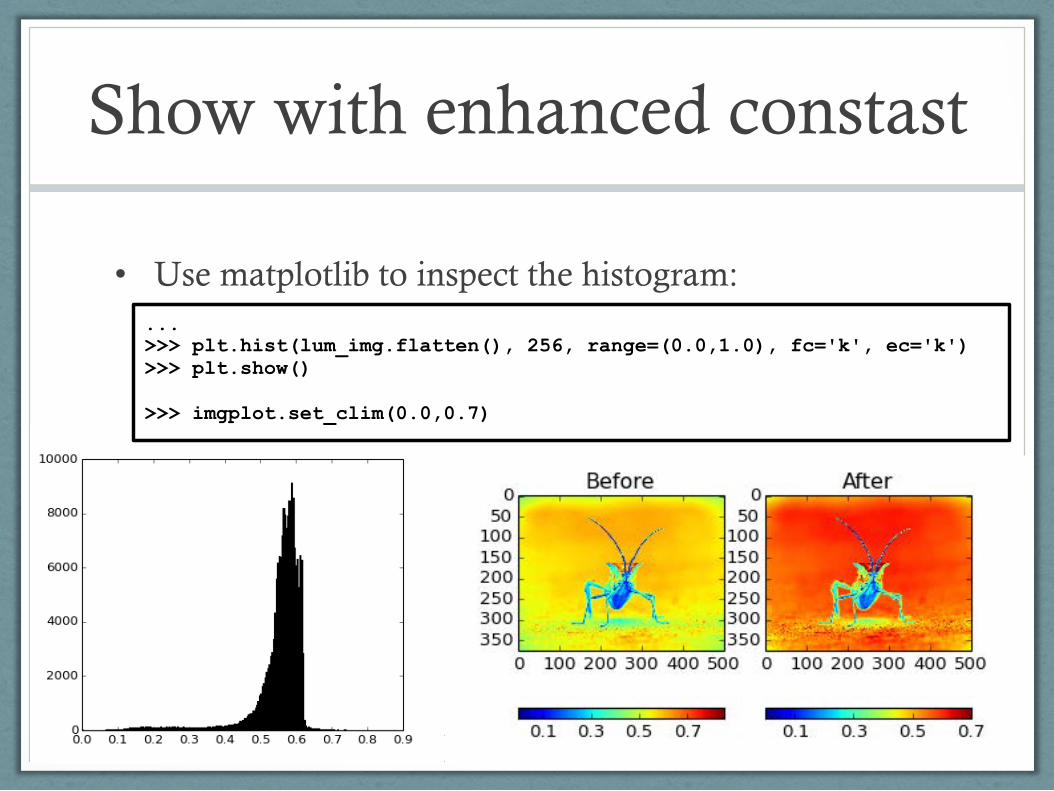
Show with enhanced constast
• Use matplotlib to inspect the histogram: ... >>> plt.hist(lum_img.flatten(), 256, range=(0.0,1.0), fc='k', ec='k') >>> plt.show() >>> imgplot.set_clim(0.0,0.7)

Visualization issue: Interpolation
• When zooming in, it may be necessary to interpolate the images pixels.
• By default, bilinear interpolation is used. It might be better to use „nearest neighbor“ interpolation to see the pixels:
• Or, for more accuracy, you may want to try bicubic interpolation:
... >>> img_plot.set_interpolation('nearest‘)
... >>> img_plot.set_interpolation(‘bicubic‘)
Working with the spyder IDE
„spyder (previously known as Pydee) is a powerful interactive development environment for the Python language with advanced editing, interactive testing, debugging and introspection features.[...]
spyder lets you easily work with the best tools of the Python scientific stack in a simple yet powerful environment.[...]“
http://code.google.com/p/spyderlib, October 2013
The screenshots of this introduction have been taken from the spyder homepage.

The spyder IDE

spyder - the editor

spyder - the console

spyder - the variable explorer

Outline Introduction
Presenting the Python programming language
Image processing with NumPy and SciPy
Visualization with matplotlib and the spyder IDE
Summary

Summary (1) The Python programming language
Readable, meaningful syntax (remember the tabs!)
Highly functional, full of functionality
Steep learning experience and fast results
Perfectly practicable for interactive work
Can be extended easily
Large global community
Summary (2) NumPy and SciPy
Efficient Array implementation
Loading and saving of images (transparently via PIL)
Adds (nature) scientific stuff to Python
Contains basic image processing functionality
Highly active and widely recommended packages

Summary (3) matplotlib
Plots everything...
Works well with NumPy arrays
spyder Nice IDE
Integrates Scientific work flow (a bit like MatLab)
Everything is there and freely available: Time to start with the excercises!

Thank you for your attention!
Time for questions, discussions etc.