Image Pyramids

Shai AvidanTel Aviv University

Slide Credits (partial list)

• Rick Szeliski• Steve Seitz• Alyosha Efros• Miki Elad• Yacov Hel-Or• Hagit Hel-Or• Marc Levoy• Bill Freeman• Fredo Durand• Sylvain Paris

Multi-resolution

• Gaussian Pyramids• Laplacian Pyramids• Other representations:

– Wavelets

– Steerable Pyramid

The Gaussian pyramid

• Synthesis – smooth and sub-sample

• Analysis– take the top image

• Gaussians are low pass filters, so representation is redundant

http://www-bcs.mit.edu/people/adelson/pub_pdfs/pyramid83.pdf

What filter to use?

∑

∑

=∀

<<∀≥

=

=

+

−

. :onContributi Equal 4.

0 : Unimodal3.

:Symmetry 2.

1 :Normalized 1.

2 constwj

jiww

ww

w

ij

ji

ii

i

1. Keeps that local image mean remains the same2. No bias in any direction3. Monotonic decrease of influence from center pixel4. Every pixel contributes equally to the next pyramid level

a+2c = 2b 2b=0.5 b=0.25 a>b=0.5 c=0.5(0.5-a)(4) (1,4) (3) (1)

The computational advantage of pyramids

http://www-bcs.mit.edu/people/adelson/pub_pdfs/pyramid83.pdf

Computational Cost

• Memory:2n x 2n(1 + ¼ + 1/16 + …) = 2n x 2n *4/3

Computation:Each level can be computed with a single convolution

Multi-scale Pattern Matching

Hierarchical pattern matching.Search in coarse level and focusefforts only on promising regions

Similarly, Hierarchical block motionestimation.

Laplacian Pyramid

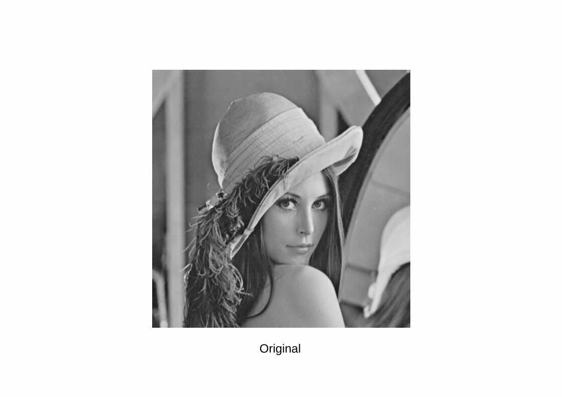
Original

Smoothed

Difference

Laplacian PyramidVersion 1:

Synthesize:P_L(0) = X – Blur(X)P_L(1) = Reduce(Blur(X))

Reconstruct:X = Expand(P_L(1)) + P_L(0) =

Expand(Reduce(Blur(X)) + X – Blur(X) != X

Laplacian PyramidVersion 2:

Synthesize:P_G(0) = XP_G(1) = Reduce(Blur(P_G(0))P_L(0) = P_G(0) – Expand(P_G(1))P_L(1) = P_G(1)

Reconstruct:X = Expand(P_L(1)) + P_L(0)

= Expand(P_G(1)) + P_G(0) – Expand(P_G(1))= Expand(Reduce(Blur(P_G(0))) + P_G(0) –

Expand(Reduce(Blur(P_G(0))) = P_G(0) = X

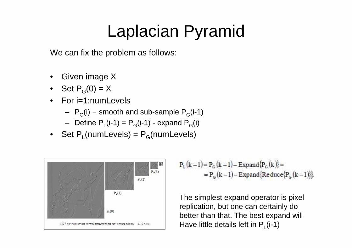
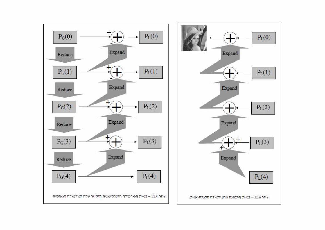
Laplacian PyramidWe can fix the problem as follows:

• Given image X• Set PG(0) = X• For i=1:numLevels

– PG(i) = smooth and sub-sample PG(i-1) – Define PL(i-1) = PG(i-1) - expand PG(i)

• Set PL(numLevels) = PG(numLevels)

The simplest expand operator is pixelreplication, but one can certainly do better than that. The best expand willHave little details left in PL(i-1)

Computational Cost

• Memory:2n x 2n(1 + ¼ + 1/16 + …) = 2n x 2n *4/3

but coefficients can be compressedComputation:

Each level can be computed with a single convolution

Image Blending

15-463: Computational PhotographyAlexei Efros, CMU, Fall 2008

© NASA

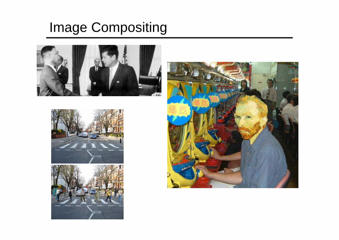
Image Compositing

Compositing Procedure1. Extract Sprites (e.g using Intelligent Scissors in Photoshop)

Composite by David Dewey

2. Blend them into the composite (in the right order)

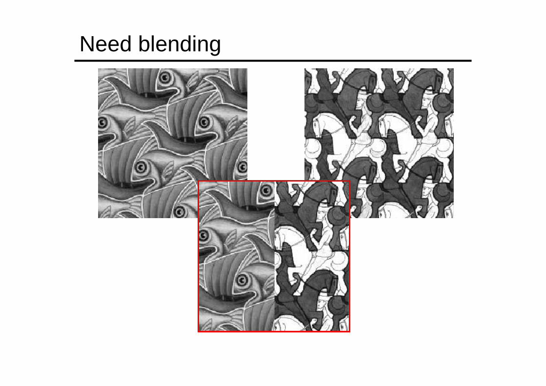
Need blending

Alpha Blending / Feathering

01

01

+

=Iblend = αIleft + (1-α)Iright

Setting alpha: simple averaging

Alpha = .5 in overlap region

Setting alpha: center seam

Alpha = logical(dtrans1>dtrans2)

DistanceTransformbwdist

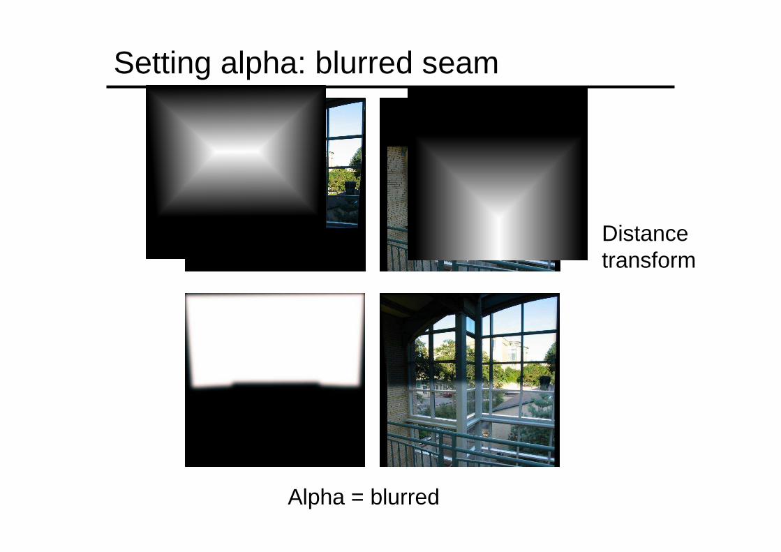
Setting alpha: blurred seam

Alpha = blurred

Distancetransform

Setting alpha: center weighting

Alpha = dtrans1 / (dtrans1+dtrans2)

Distancetransform

Ghost!

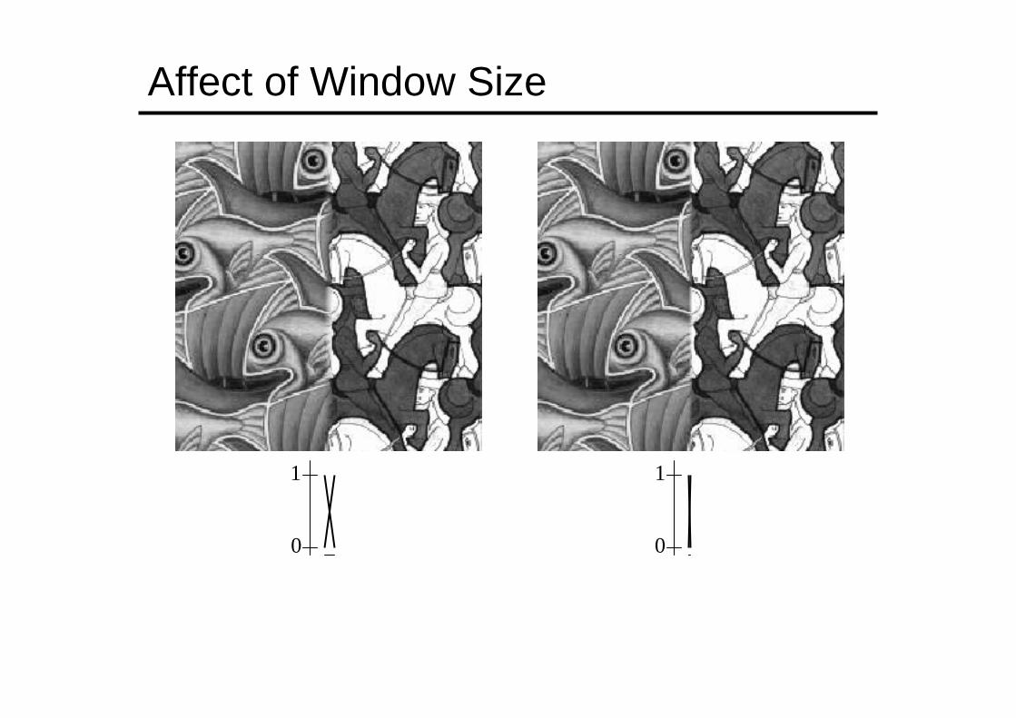
Affect of Window Size

0

1 left

right0

1

Affect of Window Size

0

1

0

1

Good Window Size

0

1

“Optimal” Window: smooth but not ghosted

What is the Optimal Window?

To avoid seams•window = size of largest prominent feature

To avoid ghosting•window <= 2*size of smallest prominent feature

Natural to cast this in the Fourier domain• largest frequency <= 2*size of smallest frequency• image frequency content should occupy one “octave” (power of two)

FFT

What if the Frequency Spread is Wide

Idea (Burt and Adelson)•Compute Fleft = FFT(Ileft), Fright = FFT(Iright)•Decompose Fourier image into octaves (bands)

–Fleft = Fleft1 + Fleft

2 + …

•Feather corresponding octaves Flefti with Fright

i

–Can compute inverse FFT and feather in spatial domain

•Sum feathered octave images in frequency domain

Better implemented in spatial domain

FFT

Octaves in the Spatial Domain

Bandpass Images

Lowpass Images

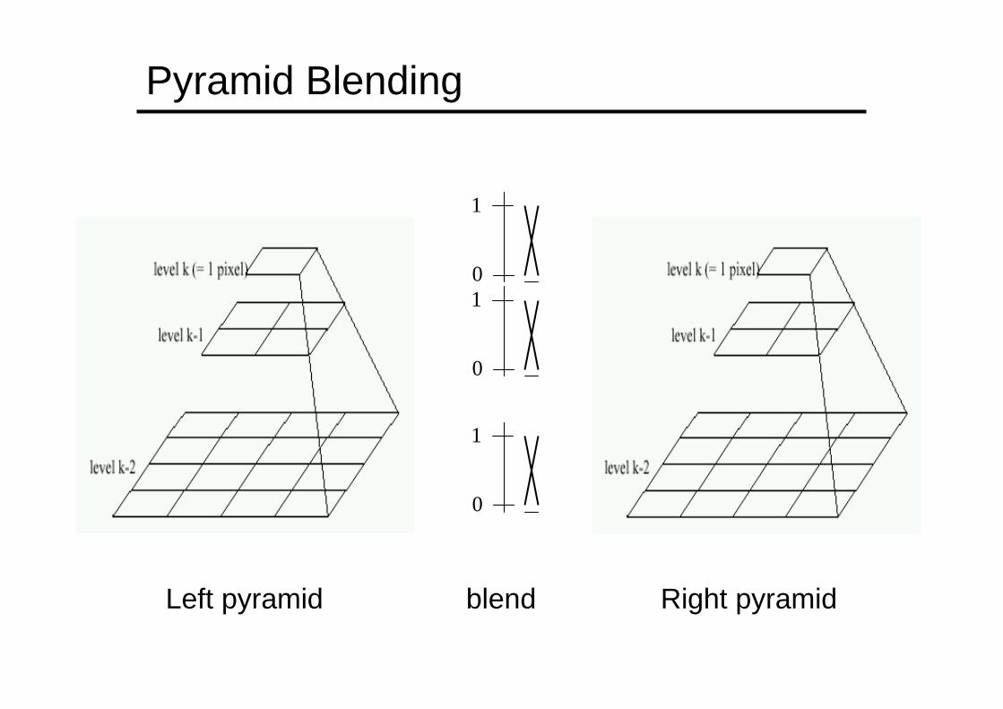
Pyramid Blending

0

1

0

1

0

1

Left pyramid Right pyramidblend

Pyramid Blending

laplacianlevel

4

laplacianlevel

2

laplacianlevel

0

left pyramid right pyramid blended pyramid

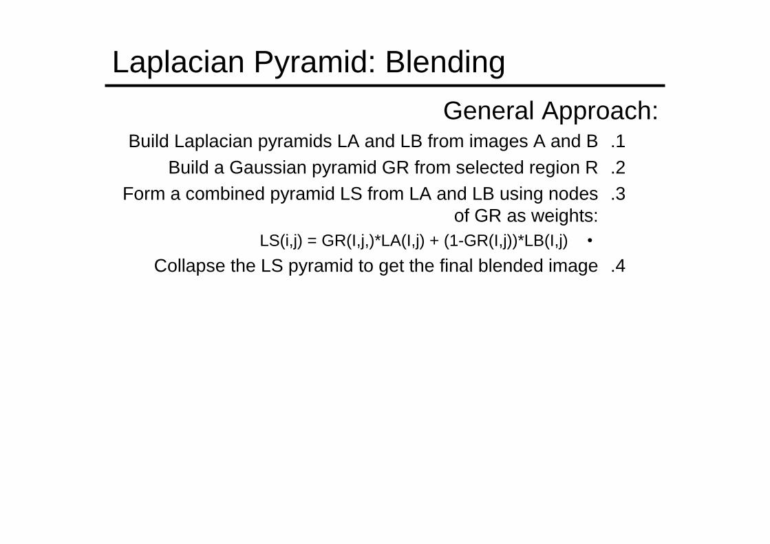
Laplacian Pyramid: Blending

General Approach:.1Build Laplacian pyramids LA and LB from images A and B.2Build a Gaussian pyramid GR from selected region R.3Form a combined pyramid LS from LA and LB using nodes

of GR as weights:•LS(i,j) = GR(I,j,)*LA(I,j) + (1-GR(I,j))*LB(I,j)

.4Collapse the LS pyramid to get the final blended image

Blending Regions

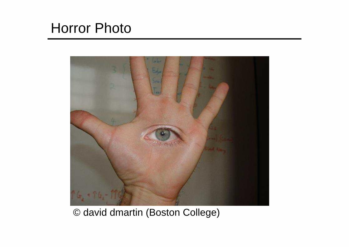
Horror Photo

© david dmartin (Boston College)

Results from this class (fall 2005)

© Chris Cameron

Season Blending (St. Petersburg)

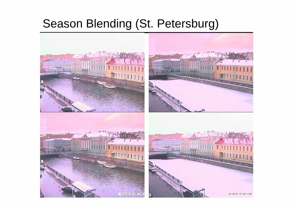
Season Blending (St. Petersburg)

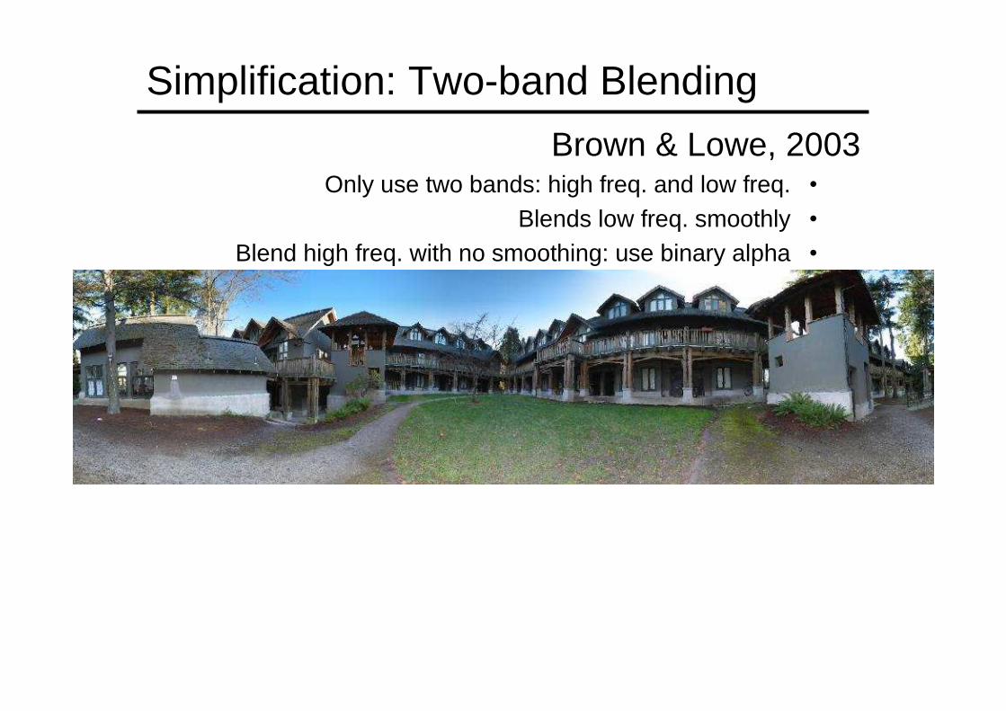
Simplification: Two-band Blending

Brown & Lowe, 2003•Only use two bands: high freq. and low freq.•Blends low freq. smoothly•Blend high freq. with no smoothing: use binary alpha

Low frequency (λ > 2 pixels)

High frequency (λ < 2 pixels)

2-band Blending

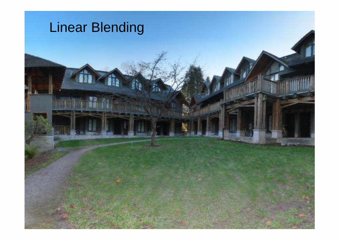
Linear Blending

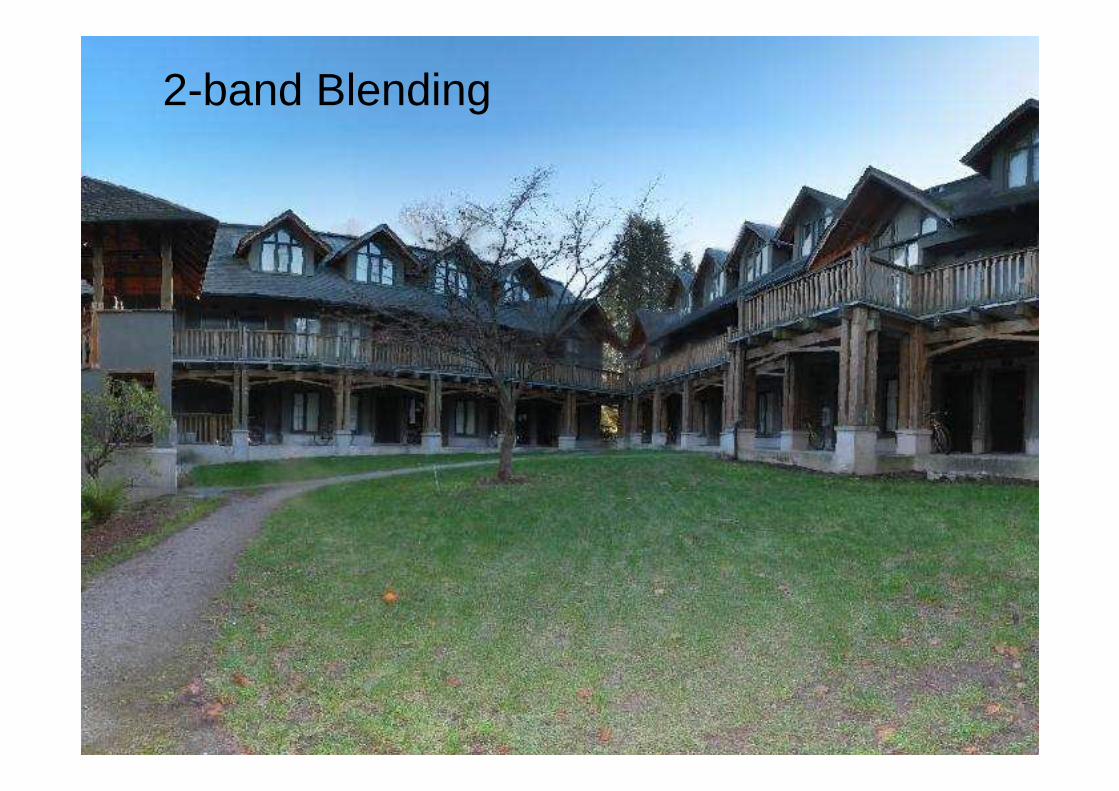
2-band Blending

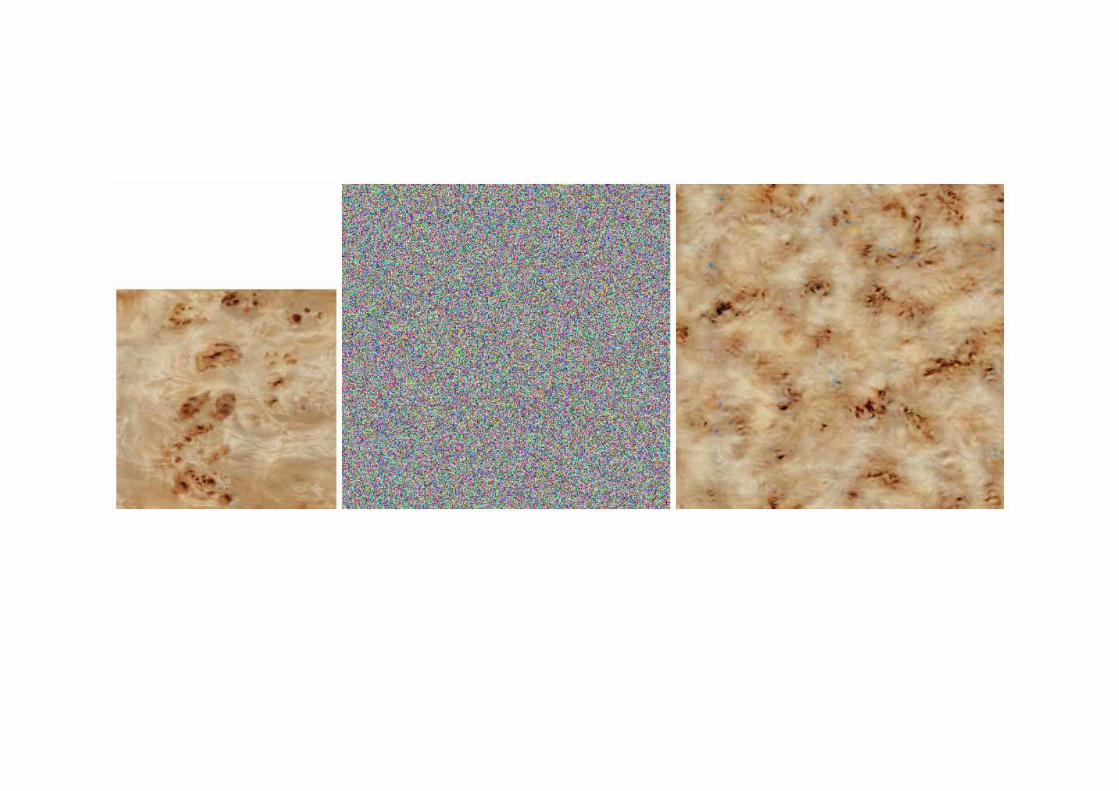
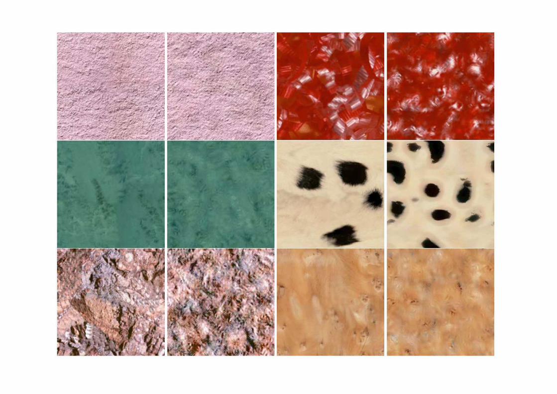
Texture SynthesisInput: Image of a textureOutput: Synthetic texture

Algorithm:

Create random image of required sizeBuild Laplacian pyramid for each

Histogram match levels of the random pyramid to the texture pyramid

Collapse pyramid of synthetic textureGo to 2

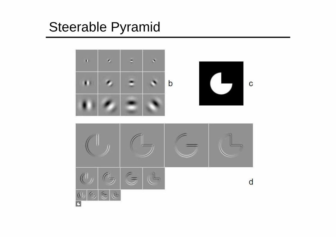
Steerable Pyramid

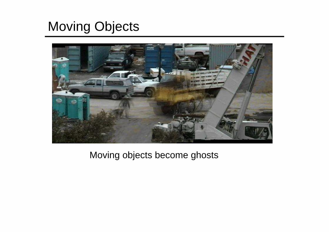
Moving Objects

Moving objects become ghosts

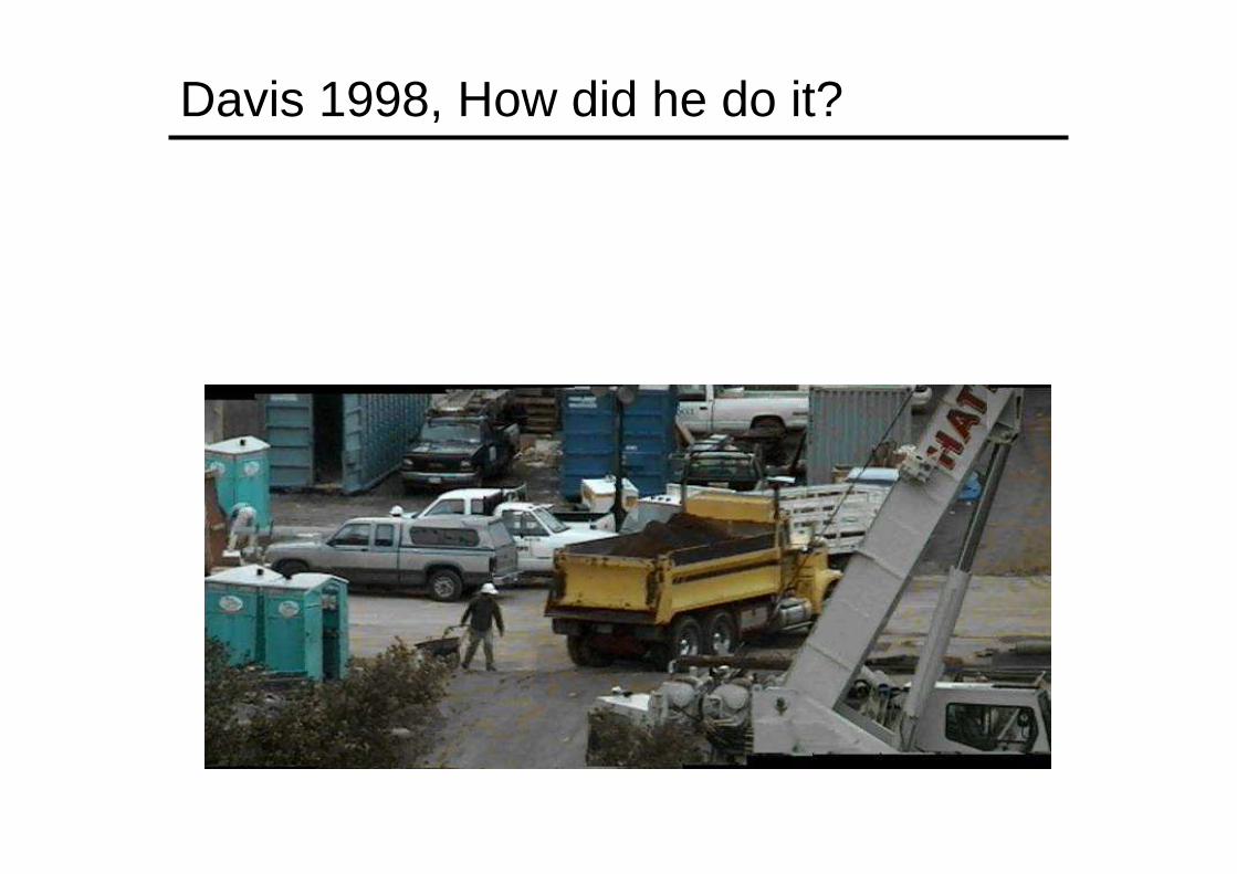
Davis 1998, How did he do it?

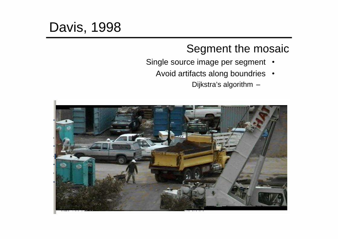
Davis, 1998

Segment the mosaic•Single source image per segment•Avoid artifacts along boundries

–Dijkstra’s algorithm

Interactive Digital PhotomontageInteractive Digital Photomontage

Aseem Agarwala, Mira Dontcheva, Maneesh Agrawala, Steven Drucker, Alex Colburn, Brian Curless, David Salesin, Michael Cohen, “Interactive Digital Photomontage”, SIGGRAPH 2004

• Combining multiple photos

• Find seams using graph cuts• Combine gradients and integrate

Algorithm DescriptionAlgorithm Description

The program operates as follows:

•The input files are read•A big blank picture is created

–The COMPOSITE

•Using graph-cut optimization algorithm–Choose good seams to combine source images

and place them on the composite

•We have N source images: S1 , ... , SN

•Choose a source image Si for each pixel p

Algorithm Description (cont.)Algorithm Description (cont.)

•Mapping between pixels and source images is a labeling L(p)

•A seam exists between two neighboring pixels p, q if L(p) ≠ L(q)

•In the inner loop at the t’th iteration:–Takes specific label α and a current labeling Lt

–Computes optimal labeling Lt+1 such that:

–Lt+1(p) = Lt (p) or Lt+1(p) = α•The outer loop iterates over each possible label

Algorithm Description (cont.)Algorithm Description (cont.)

•Terminates when passed over all labels and failed to reduce the cost function

•The cost function C of a pixel labeling L is–Sum of data penalty Cd over all pixels p–And an interaction penalty Ci over all pairs

of neighboring pixels p, q

))(),(,,())(,()(,

qLpLqpCpLpCLCqp

ip

d ∑∑ +=

Algorithm Description (cont.)Algorithm Description (cont.)

•Data penalty Cd is the distance to the image objective

–Euclidean distance in RGB space of the source image pixel SL(p)(p) from the original

composite

•Interaction Ci penalty is the distance to the seam objective

–The seam objective is 0 if L(p)=L(q)

))(),(,,())(,()(,

qLpLqpCpLpCLCqp

ip

d ∑∑ +=

Algorithm Description (cont.)Algorithm Description (cont.)

)()()()())(),(,,( )()()()( qSqSpSpSqLpLqpC qLpLqLpLi −+−=

•If L(p) ≠ L(q) then interaction penalty is:

• The algorithm employs fast approximate energy minimization via graph cuts which is called “alpha expansion”

• When this seam penalty is used, many of the theoretical guarantees of the “alpha expansion” algorithm are lost

• However, in practice the authors have found it still gives good results

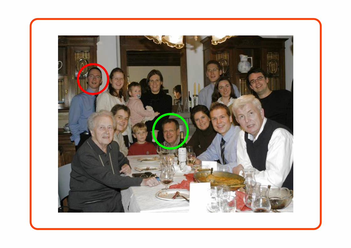
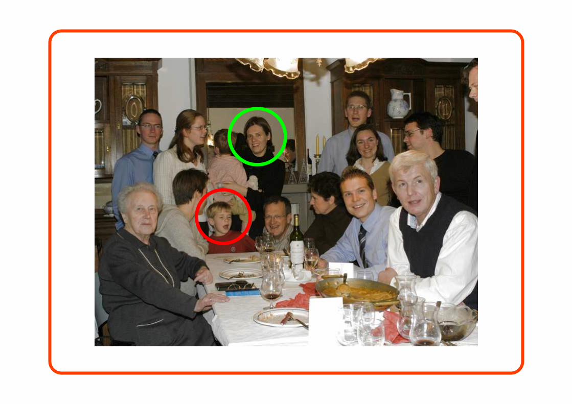
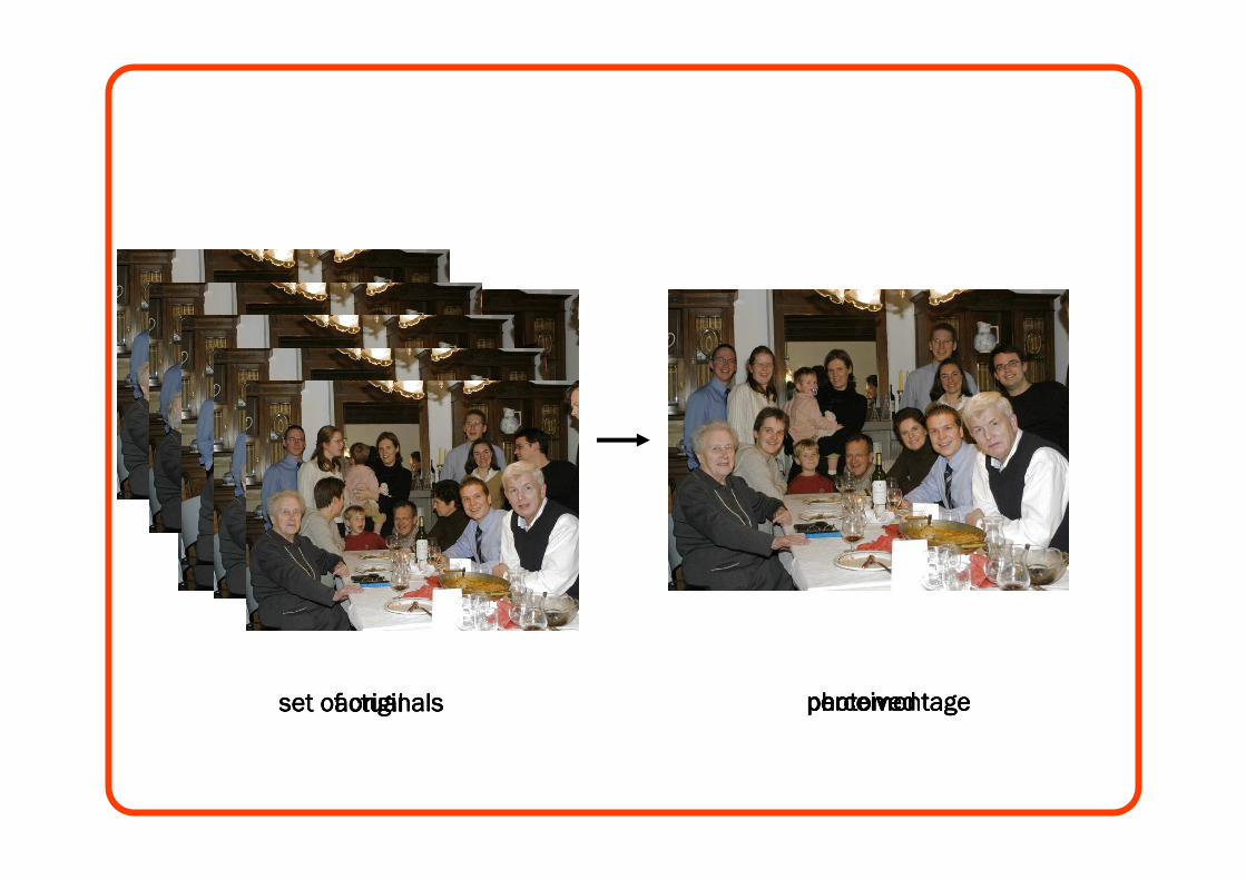
actualactualactualactual photomontagephotomontagephotomontagephotomontageset of originalsset of originalsset of originalsset of originals perceivedperceivedperceivedperceived

Source images Brush strokes Computed labeling

Composite

Brush strokes Computed labeling

Figure 2 A set of macro photographs of an ant (three of eleven used shown on the left) taken at different focal lengths. We use a global maximum contrast image objective to compute the graph-cut composite automatically (top left, with an inset to show detail, and the labeling shown directly below). A small number of remaining artifacts disappear after gradient-domain fusion (top, middle). For comparison we show composites made by Auto-Montage (top, right), by Haeberli’s method (bottom, middle), and by Laplacianpyramids (bottom, right). All of these other approaches have artifacts; Haeberli’s method creates excessive noise, Auto-Montage fails to attach some hairs to the body, and Laplacian pyramids create halos around some of the hairs.

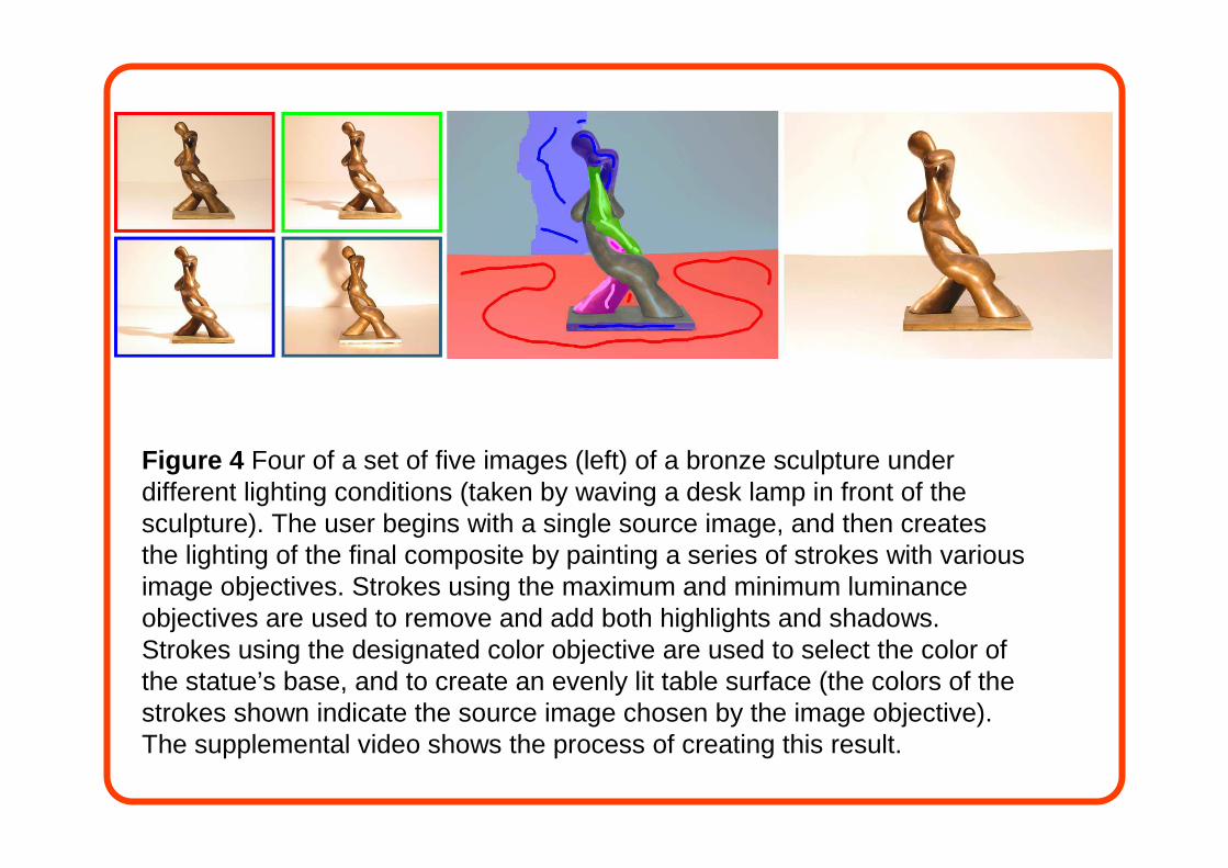
Figure 4 Four of a set of five images (left) of a bronze sculpture under different lighting conditions (taken by waving a desk lamp in front of the sculpture). The user begins with a single source image, and then creates the lighting of the final composite by painting a series of strokes with various image objectives. Strokes using the maximum and minimum luminance objectives are used to remove and add both highlights and shadows. Strokes using the designated color objective are used to select the color of the statue’s base, and to create an evenly lit table surface (the colors of the strokes shown indicate the source image chosen by the image objective). The supplemental video shows the process of creating this result.

Figure 6 We use a set of portraits (first row) to mix and match facial features, to either improve a portrait, or create entirely new people. The faces are firsthand-aligned, for example, to place all the noses in the same location. In the first two images in the second row, we replace the closed eyes of a portrait with the open eyes of another. The user paints strokes with the designated source objective to specify desired features. Next, we create a fictional person by combining three source portraits. Gradient-domain fusion is used to smooth out skin tone differences. Finally, we show two additional mixed portraits.