image reconstruction from fan-beam and cone-beam
TRANSCRIPT
Image Reconstruction from Fan-Beam andCone-Beam Projections
Bildrekonstruktion aus Facherstrahl- undKegelstrahlprojektionen
Submitted to
Technische Fakultat der
Universitat Erlangen-Nurnberg
in partial fulfillment of the requirements for
the degree of
DOKTOR-INGENIEUR
of
Frank Dennerlein
Erlangen — 2008

As dissertation accepted byTechnische Fakultat der
Universitat Erlangen-Nurnberg
Date of submission: September 8, 2008Date of doctorate: December 4, 2008Dean: Prof. Dr.-Ing. habil. Johannes HuberReviewer: Prof. Dr.-Ing. Joachim Hornegger
Frederic Noo, PhD, Associate Professor

Meinen Eltern

Abstract
This thesis addresses the problem of reconstructing static objects in 2D and 3D transmission com-puted tomography (CT). After reviewing the classical CT reconstruction theory, we discuss andthoroughly evaluate various novel reconstruction methods, two of which are original.
Our first original approach is for 2D CT reconstruction from full-scan fan-beam data, i.e., for 2Dimaging in the geometry of diagnostic medical CT scanners. Compared to conventional methods, ourapproach is computationally more efficient and also yields results with an overall reduction of imagenoise at comparable spatial resolution, as demonstrated in detailed evaluations based on simulatedfan-beam data and on data collected with a Siemens Somatom CT scanner. Part two of this thesisdiscusses the problem of 3D reconstruction in the short-scan circular cone-beam (CB) geometry,i.e., the geometry of medical C-arm systems. We first present a detailed comparative evaluation ofinnovative methods recently suggested in the literature for reconstruction in this geometry and ofthe approach applied on many existing systems. This evaluation involves various quantitative andqualitative figures-of-merit to assess image quality. We then derive an original short-scan CB recon-struction method that is based on a novel, theoretically-exact factorization of the 3D reconstructionproblem into a set of independent 2D inversion problems, each of which is solved iteratively andyields the object density on a single plane. In contrast to the state-of-the-art methods discussed ear-lier in this thesis, our factorization approach does not involve any geometric approximations duringits derivation and enforces all reconstructed values to be positive; it thus provides quantitativelyvery accurate results and effectively reduces CB artifacts in the reconstructions, as illustrated in thenumerical evaluations based on computer-simulated CB data and also real CB data acquired witha Siemens Axiom Artis C-arm system.
Kurzfassung
Diese Arbeit behandelt das Problem der Rekonstruktion statischer Objekte in der 2D und 3DTransmissions-Computertomographie (CT). Wir geben einen Uberblick der klassischen CT Rekon-struktionstheorie und diskutieren und evaluieren anschliessend mehrere neue CT Rekonstruktions-methoden; zwei dieser Methoden sind originar.
Unser erstes originares Verfahren ist fur die 2D CT Rekonstruktion aus Vollkreis-Facherstrahl-daten, das heisst, fur 2D Bildgebung in der Geometrie diagnositischer medizinischer CT Scanner.Unser Verfahren ist im Vergleich zu herkommlichen Methoden recheneffizienter und liefert aus-serdem Ergebnisse mit reduziertem Bildrauschen bei vergleichbarerer Ortsauflosung, was anhandausfuhrlicher Untersuchungen mit simulierten Daten und mit Daten eines Siemens Somatom CTScanners demonstriert wird. Teil zwei dieser Arbeit behandelt das 3D Rekonstruktionsproblem inder Teilkreis-Kegelstrahlgeometrie, das heisst, in der Geometrie medizinischer C-Bogen Systeme.Wir prasentieren eine detaillierte Vergleichsstudie innovativer Methoden, die kurzlich in der Li-teratur fur die Rekonstruktion in dieser Geometrie vorgeschlagen wurden, sowie des Verfahrens,das in vielen existierenden Systemen Anwendung findet. Unser Vergleich basiert auf quantitati-ven sowie qualitativen Bildqualitatskenngrossen. Wir leiten anschliessend eine originare Teilkreis-Kegelstrahlrekonstruktionsmethode her, die auf einer neuen, theoretisch exakten Faktorisierung des3D Rekonstruktionsproblems in eine Menge unabhangiger 2D Inversionsprobleme beruht. Jedes In-versionsproblem wird iterativ gelost und liefert die Objektdichte auf einer einzelnen Ebene. UnserFaktorisierungsverfahren bezieht im Gegensatz zu den vorher untersuchten Methoden keinerlei geo-metrische Annaherungen wahrend seiner Herleitung mit ein und erzwingt, dass alle rekonstruiertenWerte positiv sind. Es liefert daher quantitativ sehr akkurate Ergebnisse und eine effektive Reduzie-rung von Kegelstrahlartefakten, was in den numerischen Auswertungen mit simulierten Daten undmit Daten eines Siemens Axiom Artis C-Bogen Systems veranschaulicht wird.


Acknowledgement
This thesis covers some of the topics I was dealing with as a research associate at theUtah Center for Advanced Imaging Research (UCAIR) in Salt Lake City, USA. My stayabroad, from 2005 to 2008, was facilitated in the context of a research collaboration betweenthe University of Utah, the University of Erlangen-Nurnberg and Siemens AG, MedicalSolutions and I would like to express my gratitude to everyone who was involved in thisproject for the support and for valuable discussions over the years, in particular to
Prof. Dr. Frederic Noo, for his excellent supervision of my research at UCAIR and forsharing his great expertise about image reconstruction theory, and to
Prof. Dr.-Ing. Joachim Hornegger, for his guidance and motivating influence on my workdespite the large distance that separated our offices for most of the time as well as forplacing emphasis on real-data evaluations, and to
Dr. Gunter Lauritsch, for first introducing me to the exciting world of CT, for his adviceand the discussions during my semi-annual visits in Forchheim and for supporting C-armdata acquisition.
Furthermore, I would like to thank my co-workers at the Universities of Utah and Erlangen-Nurnberg and everyone I had the chance to work with over the years, for the fruitful timewe spent together during and outside working-hours. I want to thank Adam Wunderlich foracquiring and providing the 2D CT data sets that were used for the evaluation in chapter 4as well as Stefan Hoppe, Marcus Prummer and Christopher Rohkohl for their assistance inconverting and preparing the real C-arm data for the evaluations in chapter 7.
Finally, I would like to thank the Siemens AG and the NIH for providing financial supportfor my research.

Contents
1 Introduction 11.1 Computed Tomography . . . . . . . . . . . . . . . . . . . . . . . . . . . . . 11.2 CT Image Reconstruction in the Medical Environment . . . . . . . . . . . . 31.3 Scope and Original Contribution of this Thesis . . . . . . . . . . . . . . . . 41.4 Outline of this Thesis . . . . . . . . . . . . . . . . . . . . . . . . . . . . . . 5
2 The Data Model in CT 7
3 Classical Theory for Image Reconstruction in Two Dimensions 113.1 2D Radon Transform and Its Inversion . . . . . . . . . . . . . . . . . . . . . 11
3.1.1 2D Parallel-beam Geometry . . . . . . . . . . . . . . . . . . . . . . . 113.1.2 The 2D Radon Transform . . . . . . . . . . . . . . . . . . . . . . . . 123.1.3 Concept of Backprojection . . . . . . . . . . . . . . . . . . . . . . . . 153.1.4 Classical Inversion Formula for the 2D Radon Transform . . . . . . . 173.1.5 Parallel Beam Reconstruction Formula for Redundant Data . . . . . 193.1.6 Numerical Reconstruction Algorithm . . . . . . . . . . . . . . . . . . 20
3.2 2D Fan-Beam Transform and Its Classical Inversion Formula . . . . . . . . 223.2.1 The 2D Fan-Beam Geometry . . . . . . . . . . . . . . . . . . . . . . 223.2.2 The 2D Fan-Beam Transform . . . . . . . . . . . . . . . . . . . . . . 233.2.3 Classical Inversion Formula for the 2D Fan-Beam Transform . . . . 243.2.4 Numerical Reconstruction Algorithm . . . . . . . . . . . . . . . . . . 27
4 Fan-Beam Reconstruction without Backprojection Weight 294.1 Introduction . . . . . . . . . . . . . . . . . . . . . . . . . . . . . . . . . . . . 294.2 Alternative Inversion Formula for the 2D Fan-Beam Transform . . . . . . . 304.3 Fan-Beam Reconstruction with No Backprojection Weight . . . . . . . . . . 324.4 Numerical Evaluation . . . . . . . . . . . . . . . . . . . . . . . . . . . . . . 34
4.4.1 Implementation Details . . . . . . . . . . . . . . . . . . . . . . . . . 344.4.2 Evaluation of Spatial Resolution . . . . . . . . . . . . . . . . . . . . 354.4.3 Evaluation of Image Noise . . . . . . . . . . . . . . . . . . . . . . . . 384.4.4 Evaluation of Computational Efficiency . . . . . . . . . . . . . . . . 39
4.5 Reconstruction from Real CT Data . . . . . . . . . . . . . . . . . . . . . . . 434.6 Discussion and Conclusions . . . . . . . . . . . . . . . . . . . . . . . . . . . 46
5 General Theory for Image Reconstruction in Three Dimensions 495.1 3D Radon Transform and Its Inversion . . . . . . . . . . . . . . . . . . . . . 49
5.1.1 3D Radon Transform . . . . . . . . . . . . . . . . . . . . . . . . . . . 495.1.2 Analytical 3D Radon Inversion Formula . . . . . . . . . . . . . . . . 51
i
5.2 Image Reconstruction in the Cone-Beam Geometry . . . . . . . . . . . . . . 535.2.1 General Cone-beam Acquisition Geometry . . . . . . . . . . . . . . . 535.2.2 Cone-Beam Reconstruction in General . . . . . . . . . . . . . . . . . 545.2.3 The Issue of CB Data Sufficiency . . . . . . . . . . . . . . . . . . . . 565.2.4 Reconstruction via Filtered Backprojection . . . . . . . . . . . . . . 575.2.5 Reconstruction via Differentiated Backprojection . . . . . . . . . . . 58
6 Evaluation of Circular Short-Scan Reconstruction Methods 596.1 Introduction . . . . . . . . . . . . . . . . . . . . . . . . . . . . . . . . . . . . 596.2 Circular Short-Scan Geometry using a Planar Detector . . . . . . . . . . . . 606.3 The Short-Scan FDK Method . . . . . . . . . . . . . . . . . . . . . . . . . . 62
6.3.1 Reconstruction Method . . . . . . . . . . . . . . . . . . . . . . . . . 636.3.2 Implementation Details . . . . . . . . . . . . . . . . . . . . . . . . . 64
6.4 The ACE Method . . . . . . . . . . . . . . . . . . . . . . . . . . . . . . . . 646.4.1 Reconstruction Method . . . . . . . . . . . . . . . . . . . . . . . . . 646.4.2 Implementation Details . . . . . . . . . . . . . . . . . . . . . . . . . 65
6.5 The Virtual PI-Line BPF Methods . . . . . . . . . . . . . . . . . . . . . . . 666.5.1 Reconstruction Method . . . . . . . . . . . . . . . . . . . . . . . . . 676.5.2 The Virtual PI-Line BPF Method with Parker Weighting . . . . . . 686.5.3 Implementation Details . . . . . . . . . . . . . . . . . . . . . . . . . 69
6.6 Comparative Evaluation . . . . . . . . . . . . . . . . . . . . . . . . . . . . . 696.6.1 Evaluation of Spatial Resolution . . . . . . . . . . . . . . . . . . . . 706.6.2 Evaluation of Contrast-to-Noise Ratio . . . . . . . . . . . . . . . . . 746.6.3 Evaluation of CB Artifacts . . . . . . . . . . . . . . . . . . . . . . . 786.6.4 Evaluation of Impact of Axial Truncation . . . . . . . . . . . . . . . 85
6.7 Discussion and Conclusions . . . . . . . . . . . . . . . . . . . . . . . . . . . 86
7 A Factorization Method for Circular Short-Scan CB Reconstruction 897.1 Introduction . . . . . . . . . . . . . . . . . . . . . . . . . . . . . . . . . . . . 897.2 Reconstruction Theory . . . . . . . . . . . . . . . . . . . . . . . . . . . . . . 89
7.2.1 The Plane of Interest P . . . . . . . . . . . . . . . . . . . . . . . . . 897.2.2 Image Reconstruction on P . . . . . . . . . . . . . . . . . . . . . . . 917.2.3 Volume Reconstruction . . . . . . . . . . . . . . . . . . . . . . . . . 93
7.3 Numerical Algorithm . . . . . . . . . . . . . . . . . . . . . . . . . . . . . . . 957.3.1 Computation of the Intermediate Function . . . . . . . . . . . . . . 957.3.2 Discretization of the 2D Inversion Problem . . . . . . . . . . . . . . 957.3.3 Stability and Numerical Inversion Scheme . . . . . . . . . . . . . . . 97
7.4 Numerical Studies . . . . . . . . . . . . . . . . . . . . . . . . . . . . . . . . 1007.4.1 Experimental Set-Up . . . . . . . . . . . . . . . . . . . . . . . . . . . 1007.4.2 Impact of Parameter α on Image Quality . . . . . . . . . . . . . . . 1007.4.3 Impact of Parameter σ on Image Quality . . . . . . . . . . . . . . . 103
7.5 Comparative Evaluation of the Factorization Method . . . . . . . . . . . . . 1037.5.1 Comparison of Spatial Resolution and Image Noise . . . . . . . . . . 1047.5.2 Comparison of CB Artifacts . . . . . . . . . . . . . . . . . . . . . . . 1067.5.3 Comparison of Axial Truncation Artifacts . . . . . . . . . . . . . . . 110
7.6 Reconstruction from Real C-arm Data . . . . . . . . . . . . . . . . . . . . . 1117.6.1 Acquisition Geometry of a Real C-arm System . . . . . . . . . . . . 1117.6.2 Handling of Real C-arm CB Data . . . . . . . . . . . . . . . . . . . . 1127.6.3 Reconstruction Results . . . . . . . . . . . . . . . . . . . . . . . . . . 113
ii

7.7 Discussion and Conclusions . . . . . . . . . . . . . . . . . . . . . . . . . . . 115
8 Conclusions and Outlook 117
List of Symbols and Acronyms 125
List of Figures 127
List of Tables 131
iii

iv
Chapter 1
Introduction
1.1 Computed Tomography
This thesis addresses specific research topics in the field of recovering human body struc-tures from X-ray projection data in medical examination. The historical starting point tothis examination method can be traced back into the 1890s, when the high-energetic electro-magnetic rays that are nowadays known as X-rays were discovered [8]. One of the pioneerswho carried out first experiments was the German physicist Wilhelm Conrad Roentgen,who was able to generate and measure X-rays and who managed to demonstrate, in 1895,that these rays, which are able to traverse most solid objects, can be used to create pho-tographic impressions of interior object structures that are otherwise hidden to the humaneye [77]. This was an exciting discovery [8], and over the years, examination of objects usingX-rays has found its way into various fields of application, including the field of securitysystems, the field of non-destructive evaluation of industrial objects and – in particular –the field of medical imaging [71].
In the early days of X-ray examination and also in the contemporary application, thefundamental design of systems used for X-ray examination is based on the following concept:X-rays are generated in a ray source, sent through the object under investigation, so thatthey project the object structure onto some X-ray sensitive material, such as chemical film,that transforms incoming X-radiation into an image. Hence, the natural capability of X-ray systems is to acquire projection images of the investigated object and these projectionscan be collected from one or more viewing directions, as desired. The individual imagesmay then be interpreted by a specialist and for a long time, this described examinationmethod, known as projection radiography, was the method commonly used in the practicalapplication [30, 85].
Over the last few decades, however, X-ray examination systems have become more andmore sophisticated [30, 48]. Electronic control, for instance, allows the user to approachdifferent viewing directions quickly, automatically and with high precision. Nowadays,projection images can be acquired using high-resolution digital detectors that involve semi-conductor technology instead of using chemical film [71]. These and other refinements in themechanical design and the acquisition process naturally created a desire for more compleximaging applications [30, 71, 70], such as
i) quantitative measurements, for instance, precise determination of the density, thelength or the volume of structures within the investigated object,
1
2 Chapter 1. Introduction
ii) volumetric visualization, for instance, graphically illustrating the 3D surface of theobject or of parts of the object, possibly using specific color schemes to encode addi-tional information, or
iii) computer-aided image interpretation, for instance, assisting the user in detectingor locating specific features in the investigated object.
These applications significantly increase the practical benefit of X-ray examination systems,but they require information about the actual structure of the object; pure knowledge aboutindividual projection images, as can be collected with an X-ray system, is not sufficient.Hence there is some discrepancy between the information that can be naturally obtainedduring examination and the information needed to carry out the desired applications listedabove. This discrepancy is effectively tackled by the concepts of transmission computedtomography (CT) .
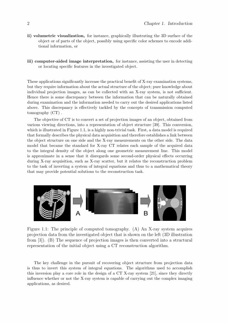
The objective of CT is to convert a set of projection images of an object, obtained fromvarious viewing directions, into a representation of object structure [39]. This conversion,which is illustrated in Figure 1.1, is a highly non-trivial task. First, a data model is requiredthat formally describes the physical data acquisition and therefore establishes a link betweenthe object structure on one side and the X-ray measurements on the other side. The datamodel that became the standard for X-ray CT relates each sample of the acquired datato the integral density of the object along one geometric measurement line. This modelis approximate in a sense that it disregards some second-order physical effects occurringduring X-ray acquisition, such as X-ray scatter, but it relates the reconstruction problemto the task of inverting a system of integral equations and thus to a mathematical theorythat may provide potential solutions to the reconstruction task.
Figure 1.1: The principle of computed tomography. (A) An X-ray system acquiresprojection data from the investigated object that is shown on the left (3D illustrationfrom [3]). (B) The sequence of projection images is then converted into a structuralrepresentation of the initial object using a CT reconstruction algorithm.
The key challenge in the pursuit of recovering object structure from projection datais thus to invert this system of integral equations. The algorithms used to accomplishthis inversion play a core role in the design of a CT X-ray system [21], since they directlyinfluence whether or not the X-ray system is capable of carrying out the complex imagingapplications, as desired.
1.2. CT Image Reconstruction in the Medical Environment 3
1.2 CT Image Reconstruction in the Medical En-
vironment
The concepts of CT have been applied on medical imaging systems for more than 30 years.One of the first prototype systems for CT imaging was developed by Godfrey Hounsfieldand first commercially-available systems were introduced by the British company EMI [12].Since then, the CT technology contributed to significant advancements in medical diagnosisand intervention by providing improved or entirely new imaging techniques; examples ofthese techniques are given, for instance, in [48, 70, 71, 59].
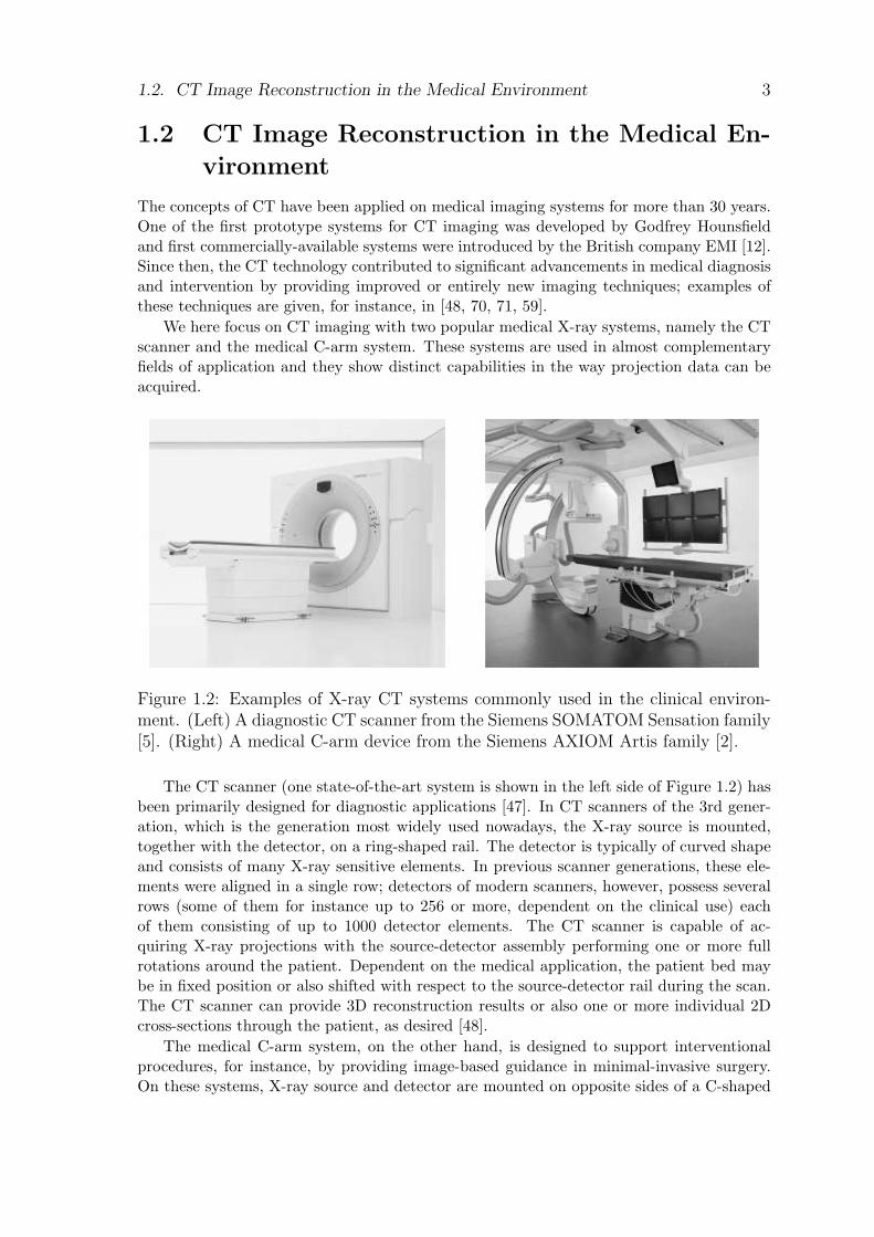
We here focus on CT imaging with two popular medical X-ray systems, namely the CTscanner and the medical C-arm system. These systems are used in almost complementaryfields of application and they show distinct capabilities in the way projection data can beacquired.
Figure 1.2: Examples of X-ray CT systems commonly used in the clinical environ-ment. (Left) A diagnostic CT scanner from the Siemens SOMATOM Sensation family[5]. (Right) A medical C-arm device from the Siemens AXIOM Artis family [2].
The CT scanner (one state-of-the-art system is shown in the left side of Figure 1.2) hasbeen primarily designed for diagnostic applications [47]. In CT scanners of the 3rd gener-ation, which is the generation most widely used nowadays, the X-ray source is mounted,together with the detector, on a ring-shaped rail. The detector is typically of curved shapeand consists of many X-ray sensitive elements. In previous scanner generations, these ele-ments were aligned in a single row; detectors of modern scanners, however, possess severalrows (some of them for instance up to 256 or more, dependent on the clinical use) eachof them consisting of up to 1000 detector elements. The CT scanner is capable of ac-quiring X-ray projections with the source-detector assembly performing one or more fullrotations around the patient. Dependent on the medical application, the patient bed maybe in fixed position or also shifted with respect to the source-detector rail during the scan.The CT scanner can provide 3D reconstruction results or also one or more individual 2Dcross-sections through the patient, as desired [48].
The medical C-arm system, on the other hand, is designed to support interventionalprocedures, for instance, by providing image-based guidance in minimal-invasive surgery.On these systems, X-ray source and detector are mounted on opposite sides of a C-shaped
4 Chapter 1. Introduction
arm and the mechanical design of this arm is focussed on providing very flexible motionaround the patient bed. The C-arm system differs in some aspects fundamentally fromthe diagnostic CT scanner. C-arm systems, for instance, do not in general allow X-rayprojections to be acquired along a full rotation around the patient. Also, modern C-armsystems possess a large, digital flat-panel detector that, e.g., consists of several millionX-ray sensitive elements arranged in a 2D grid that covers an area of about 30 cm×40 cm[2]. Another important fact is that C-arm systems were initially designed exclusively foracquiring 2D projections from various points of view [60] – the concepts of 3D CT wereintroduced as a standard feature of C-arm systems in the late 1990s [88].
The practical benefit of these two medical CT systems depends on the quality of theimage reconstruction. For a long time, image quality issues were dominated not by thereconstruction algorithm but by the fact that the physical processes during data acquisitiondeviate to some respect from the data assumptions of the reconstruction algorithm – thisinconsistency yields reconstruction artifacts. However, due to improvements in hardwareand data processing, this mismatch between the data model and physical reality was reducedsuccessively so that nowadays, the performance of the reconstruction algorithm becomesincreasingly decisive for the resulting image quality. Considering the fact that CT imagereconstruction on many existing systems is carried out using methods that are variations ofapproaches introduced more than 20 years ago [71], the consideration of novel reconstructionapproaches may be the key for improving the overall system performance.
1.3 Scope and Original Contribution of this Thesis
In this thesis, we present and thoroughly evaluate various novel approaches to achieve imagereconstruction from static objects on medical X-ray CT systems. The new methods comewith advantages in image quality and/or efficiency compared to the conventional approachesthat are typically considered in existing CT systems. Two of these presented methods areoriginal and some of their concepts have been published in peer-reviewed journals; see[27, 29].
In the first part of this thesis, we derive and evaluate a novel analytic method for 2Dimage reconstruction from projection data measured in the geometry of the diagnostic CTscanner. Our novel approach is primarily designed to be computationally more efficientcompared to classical approaches, by avoiding the application of a specific weighting factorduring computation. In addition to that, it also yields improvements in the noise char-acteristics of the resulting images without noticeably sacrificing resolution. In the secondpart of this thesis, we consider 3D image reconstruction in the geometry of medical C-armsystems and present, in a uniform way, three methods recently suggested in the literature toaccomplish that task. We describe a methodology for detailed comparison of image qualityin C-arm CT and use this methodology to compare these three reconstruction methodsto each other, but also to the reconstruction method currently in use in many existingC-arm systems. We then derive a novel, original approach for image reconstruction fromC-arm data that comes along without any geometric approximations during its derivation,in contrast to the methods described before. It thus aims at achieving higher accuracy inthe reconstruction results, in particular compared to the method currently used in mostC-arm systems. Our new method involves analytic steps and also a 2D iterative scheme torecover 3D object density, and is furthermore designed to naturally cope with some degreeof truncation in the acquired projection images.
1.4. Outline of this Thesis 5
Each of the two original reconstruction methods that we present in this thesis is carefullyderived from known theory, thoroughly numerically evaluated against other competitivemethods using computer-simulated CB data and also tested for image reconstruction fromprojection data acquired with commercially-available X-ray CT systems.
1.4 Outline of this Thesis
This thesis is structured as follows. Chapter 2 describes the standard CT data model,which is a prerequisite for the considerations in the subsequent chapters. The main bodyof this thesis, which follows this introductory chapter, is divided into two parts that areabout image reconstruction in the 2D scenario (chapters 3 and 4) and in the 3D scenario(chapters 5, 6 and 7), respectively. Each of these parts starts with a chapter that reviews theclassical theory of image reconstruction in the respective scenario. In these review chapters,we give derivations of the fundamental concepts wherever appropriate, and also presentnumerical examples to illustrate the corresponding theory. In the subsequent chapters ofeach part we thoroughly present our original contributions, in the following sequence:
Chapter 4 presents our novel, original filtered-backprojection method for 2D image re-construction in the geometry of the diagnostic CT-scanner. In sections 4.2 and 4.3, we deriveour method and point out its differences from the conventional approaches. Our novel ap-proach is thoroughly evaluated and compared to the analytic reconstruction method of Nooet al. [67] in section 4.4. The evaluation is based on computer-simulated data and carriedout in terms of spatial resolution, image noise and computational efficiency. Section 4.5presents an evaluation based on real projection data acquired with a commercially-availableCT scanner. Final discussions and conclusions are given in section 4.6.
Chapter 6 is focussed on 3D image reconstruction in the circular short-scan cone-beamacquisition geometry with a flat detector, i.e., in the geometry of most modern C-arm sys-tems, which is formally introduced in section 6.2. We then present four state-of-the-artmethods suggested for image reconstruction from short-scan circular cone-beam data, insections 6.3, 6.4 and 6.5, and compare the image quality achievable with these methodsin section 6.6. Our comparative image quality study is based on a uniform evaluationframework and carried out in terms of spatial resolution (section 6.6.1), contrast-to-noiseratio (section 6.6.2), cone-beam artifacts (section 6.6.3) and axial truncation artifacts (sec-tion 6.6.4). Section 6.7 gives conclusions and discussions about our comparison study.
Chapter 7 presents our novel, original factorization approach for circular short-scancone-beam reconstruction. The general theoretical background of our method is illustratedin section 7.2. We then suggest, in section 7.3, a numerical scheme to implement from thistheory a practical cone-beam reconstruction algorithm. The performance of this factoriza-tion algorithm is then evaluated and compared to that of the methods described earlier inthis thesis. Section 7.6 is about reconstruction from cone-beam data collected with a clinicalC-arm system. It first describes specific aspects of the geometry of existing C-arm systemsand presents modifications we considered in our algorithm to cope with these geometricaspects. Reconstruction results of a physical thorax phantom are shown in section 7.6.3and final discussions on our factorization approach are given in section 7.7.
In the final chapters of this thesis, we present an overall conclusion about our researchand give an outlook about possible future theoretical and algorithmic developments of thespecific topics discussed in this thesis and of the field of CT image reconstruction in general.Note finally that we use a notation scheme where a symbol is in general restricted to the

6 Chapter 1. Introduction
chapter in which it is introduced. Some symbols are, however, used throughout variouschapters; these symbols are summarized in the glossary at the end of this thesis.
Chapter 2
The Data Model in CT
This chapter briefly describes the standard data model of X-ray CT, i.e., the model used toestablish a formal relation between the measured data and the object under investigation.This formal relation is essential for the development of reconstruction algorithms, and thusalso forms the backbone of the algorithms discussed in the following chapters.
Projection data acquired with modern CT systems is the result of an X-ray sourcethat emits X-ray photons and many X-ray sensitive detector elements with each elementmeasuring incoming radiation. Clearly, source and detector elements need to be locatedon distinct sides of the investigated object; in medical CT devices, which are the focus ofthis thesis, the distance between these two entities is about 1 to 1.5 meters, thus providingenough space for the patient to be conveniently placed in between. Compared to thisgeometric scale, both the X-ray focal spot and each considered detector element are tinyobjects with typically only about one millimeter width and length [71].
Let us focus on one arbitrary sample of the X-ray data set from now on, i.e., on themeasurement obtained at one single detector element at one point in time; the formal de-scription of this data sample is based on a simplification on the real physical processes.First, it is assumed that both, focal spot of the X-ray source and the considered detectorelement are punctiform. In other words, X-ray photons are assumed to diverge from an in-finitessimately small area centered on the actual X-ray focal spot and all photons registeredby the detector element are assumed to pass through the central point on that finite sizedetector region. The ray that connects the points representing X-ray source and detectorelement will be referred to as a measurement ray in the following and will be denoted usingthe symbol L. It is furthermore assumed that the source emits monochromatic X-radiationand that the direction in which each X-ray photon advances in space remains unchangedafter emission. The number of photons sent from the source point along the considered lineL will be denoted by the integer NS and the amount of photons eventually registered atthe detector element as ND. The ratio of these two photon counts, ND and NS , containsinformation about the attenuation characteristic of the material along L as will becomeclearer below.
Let the value µ ≥ 0 denote the linear X-ray attenuation coefficient of the investigatedobject. Values of µ are commonly expressed in a scale (the Hounsfield scale [71]) that is de-fined relative to the attenuation of water, for which we use the value µwater = 0.01836mm−1
throughout this thesis. The linear attenuation coefficient is converted into values of theHounsfield scale as [47]
µ− µwater
µwater× 1000. (2.1)
7
8 Chapter 2. The Data Model in CT
Consequently, the absence of attenuating material corresponds to a value of−1000 Hounsfieldunits (HU), while the attenuation of water is given, for instance, as 0 HU. The attenuationcoefficients of important structures of the human body, such as those of bones or of differentorgans, are given in [71].
Beer’s law [71] then introduces the following relation between the object attenuationcoefficient and the X-ray photon measurements:
ND = NS e−
tD∫tS
µL(t) dt
. (2.2)
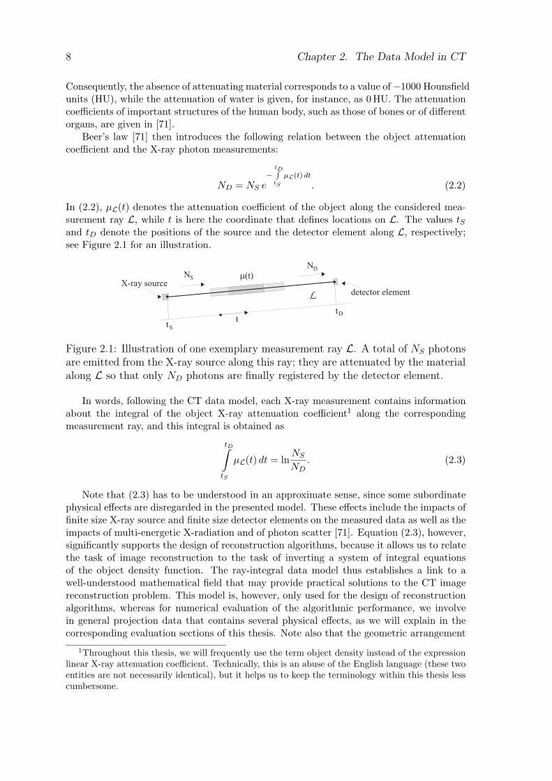
In (2.2), µL(t) denotes the attenuation coefficient of the object along the considered mea-surement ray L, while t is here the coordinate that defines locations on L. The values tSand tD denote the positions of the source and the detector element along L, respectively;see Figure 2.1 for an illustration.
Figure 2.1: Illustration of one exemplary measurement ray L. A total of NS photonsare emitted from the X-ray source along this ray; they are attenuated by the materialalong L so that only ND photons are finally registered by the detector element.
In words, following the CT data model, each X-ray measurement contains informationabout the integral of the object X-ray attenuation coefficient1 along the correspondingmeasurement ray, and this integral is obtained as
tD∫
tS
µL(t) dt = lnNS
ND. (2.3)
Note that (2.3) has to be understood in an approximate sense, since some subordinatephysical effects are disregarded in the presented model. These effects include the impacts offinite size X-ray source and finite size detector elements on the measured data as well as theimpacts of multi-energetic X-radiation and of photon scatter [71]. Equation (2.3), however,significantly supports the design of reconstruction algorithms, because it allows us to relatethe task of image reconstruction to the task of inverting a system of integral equationsof the object density function. The ray-integral data model thus establishes a link to awell-understood mathematical field that may provide practical solutions to the CT imagereconstruction problem. This model is, however, only used for the design of reconstructionalgorithms, whereas for numerical evaluation of the algorithmic performance, we involvein general projection data that contains several physical effects, as we will explain in thecorresponding evaluation sections of this thesis. Note also that the geometric arrangement
1Throughout this thesis, we will frequently use the term object density instead of the expressionlinear X-ray attenuation coefficient. Technically, this is an abuse of the English language (these twoentities are not necessarily identical), but it helps us to keep the terminology within this thesis lesscumbersome.

9
of all measurement rays occurring during the X-ray CT data acquisition significantly deter-mines both feasibility and difficulty of this reconstruction task [39], as will become clearerin the following chapters.

10 Chapter 2. The Data Model in CT
Chapter 3
Classical Theory for ImageReconstruction in Two Dimensions
This chapter introduces the classical theory about reconstruction of 2D objects from 1Dprojection data. The plane on which these objects are defined will be referred to as the imageplane from now on. A Cartesian, right-handed world coordinate system with coordinatesx and y is introduced on the image plane such that an arbitrary position can be addressedusing the coordinate vector x = (x, y)T. Note that here and throughout the rest of thisthesis, the superscript T denotes the transpose of a matrix or vector.
The spatial density distribution of the investigated object on the 2D image plane willbe described using the function f(x). It is assumed that the object is of finite size andfurthermore approximately centered on the origin of the world coordinate system. Morespecifically, the object is assumed to fit entirely into a circular region of radius Ro aroundthe world coordinate origin; this region will be denoted as Ωf from now on, so that
f(x) = 0 for all x /∈ Ωf := x |√
x2 + y2 ≤ Ro. (3.1)
3.1 2D Radon Transform and Its Inversion
Section 3.1 deals with the problem of image reconstruction from integral data that is ac-quired with measurement lines aligned parallel to each other. This specific scenario corre-sponds to the least complex geometry discussed in this thesis and is referred to as the 2Dparallel-beam geometry from now on. Note that direct data acquisition in this geometry isnot very practical and has only be considered in CT scanners of the first generation [47].However, this scenario is interesting from a theoretical perspective, because image recon-struction in the 2D parallel-beam geometry is a direct application of the theory of Radonintegral transforms [46] that has been introduced by Johann Radon in 1917 [76].
3.1.1 2D Parallel-beam Geometry
Consider an arbitrary set of parallel lines in the image plane. This set may be specified,following the scheme used in [4], by the unit vector θ = (cos θ, sin θ)T that is perpendicularto all lines in the set. In this notation, parameter θ corresponds to the angle that vectorθ describes with the x-axis, measured in counterclockwise direction. One specific elementamong all lines in the set defined by any θ can be addressed by its signed distance s ∈ R
11
12 Chapter 3. Classical Theory for Image Reconstruction in Two Dimensions
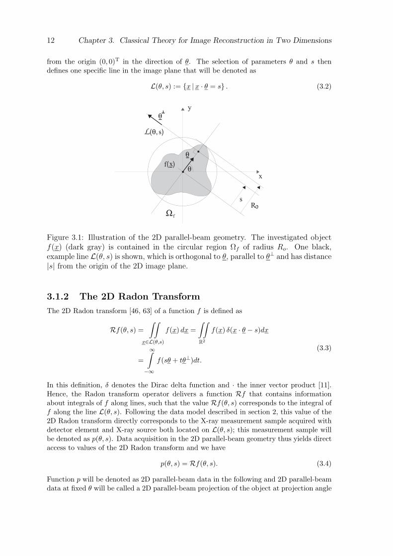
from the origin (0, 0)T in the direction of θ. The selection of parameters θ and s thendefines one specific line in the image plane that will be denoted as
L(θ, s) := x |x · θ = s . (3.2)
y
R
x
s
f x
s
f
Figure 3.1: Illustration of the 2D parallel-beam geometry. The investigated objectf(x) (dark gray) is contained in the circular region Ωf of radius Ro. One black,example line L(θ, s) is shown, which is orthogonal to θ, parallel to θ⊥ and has distance|s| from the origin of the 2D image plane.
3.1.2 The 2D Radon Transform
The 2D Radon transform [46, 63] of a function f is defined as
Rf(θ, s) =∫∫
x∈L(θ,s)
f(x) dx =∫∫
R2
f(x) δ(x · θ − s)dx
=
∞∫
−∞f(sθ + tθ⊥)dt.
(3.3)
In this definition, δ denotes the Dirac delta function and · the inner vector product [11].Hence, the Radon transform operator delivers a function Rf that contains informationabout integrals of f along lines, such that the value Rf(θ, s) corresponds to the integral off along the line L(θ, s). Following the data model described in section 2, this value of the2D Radon transform directly corresponds to the X-ray measurement sample acquired withdetector element and X-ray source both located on L(θ, s); this measurement sample willbe denoted as p(θ, s). Data acquisition in the 2D parallel-beam geometry thus yields directaccess to values of the 2D Radon transform and we have
p(θ, s) = Rf(θ, s). (3.4)
Function p will be denoted as 2D parallel-beam data in the following and 2D parallel-beamdata at fixed θ will be called a 2D parallel-beam projection of the object at projection angle
3.1. 2D Radon Transform and Its Inversion 13
θ. Clearly, any line L(θ, s) with |s| > Ro has no intersection with the object due to theinitial assumption (3.1), and consequently
p(θ, s) = 0 for |s| > Ro. (3.5)
Therefore, if p(θ, s) is given for all s ∈ [−Ro, Ro], the entire set of potentially non-zerovalues of the 2D Radon transform of f at parameter θ are known. The 2D parallel-beamprojection at the corresponding projection angle will be called non-truncated from now on.
Consider the following example for an illustration of the 2D Radon transform operator[4]. Let
fcirc(x) =
1 if
√x2 + y2 ≤ Rcirc
0 otherwise(3.6)
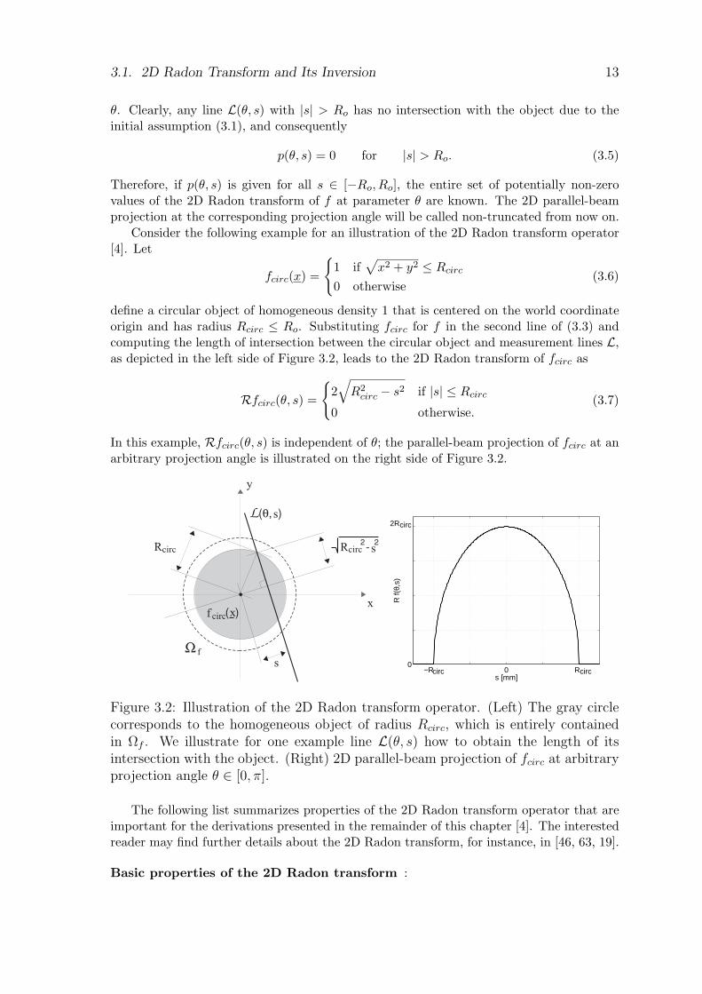
define a circular object of homogeneous density 1 that is centered on the world coordinateorigin and has radius Rcirc ≤ Ro. Substituting fcirc for f in the second line of (3.3) andcomputing the length of intersection between the circular object and measurement lines L,as depicted in the left side of Figure 3.2, leads to the 2D Radon transform of fcirc as
Rfcirc(θ, s) =
2√
R2circ − s2 if |s| ≤ Rcirc
0 otherwise.(3.7)
In this example, Rfcirc(θ, s) is independent of θ; the parallel-beam projection of fcirc at anarbitrary projection angle is illustrated on the right side of Figure 3.2.
Rcirc s
x
y
f
Rcirc
s
s
circf x
−Rcirc 0 Rcirc0
2Rcirc
s [mm]
R f(
θ,s)
Figure 3.2: Illustration of the 2D Radon transform operator. (Left) The gray circlecorresponds to the homogeneous object of radius Rcirc, which is entirely containedin Ωf . We illustrate for one example line L(θ, s) how to obtain the length of itsintersection with the object. (Right) 2D parallel-beam projection of fcirc at arbitraryprojection angle θ ∈ [0, π].
The following list summarizes properties of the 2D Radon transform operator that areimportant for the derivations presented in the remainder of this chapter [4]. The interestedreader may find further details about the 2D Radon transform, for instance, in [46, 63, 19].
Basic properties of the 2D Radon transform :
14 Chapter 3. Classical Theory for Image Reconstruction in Two Dimensions
• Linearity:
R(
N∑
i=1
cifi
)(θ, s) =
N∑
i=1
ciRfi(θ, s) (3.8)
• Periodicity:Rf(θ + 2πk, s) = Rf(θ, s); k ∈ Z (3.9)
• Redundancy:Rf(θ + π,−s) = Rf(θ, s) (3.10)
The linearity of the operator R follows from its definition in (3.3) and from thelinearity of the integral operation. The 2π periodicity in θ and the redundancyproperty, on the other hand, are a direct result from (3.3) and from the characteristicsof the involved trigonometric functions.
2D Radon transform and object modification :
• Object translation:The 2D Radon transform of objects f(x) and f0(x) that are related to each otherthrough a translation with the translation vector x0, such that f(x) = f0(x−x0),satisfies the following relation [4]:
Rf(θ, s) =∫∫
R2
f0(x− x0)δ(x · θ − s) dx
=∫∫
R2
f0(x′)δ(x′ · θ + x0 · θ − s) dx′
=∫∫
R2
f0(x′)δ(x′ · θ − (s− x0 · θ)) dx′
=Rf0(θ, s− x0 · θ).
(3.11)
• Linear object distortion:If the object f can be related to a reference object f0 through a non-singularlinear transformation, such as a rotation or a dilation, i.e., if f(x) = f0(Ax)with A ∈ R2×2 and detA 6= 0, it can be shown that
Rf(θ, s) =∫∫
R2
f0(Ax)δ(x · θ − s)dx
=1
detA
∫∫
R2
f0(x′)δ(A−1x′ · θ − s)dx′
=1
detA
∫∫
R2
f0(x′)δ(x′ ·A−T θ − s)dx′
=1
detA1
‖A−T θ‖∫∫
R2
f0(x′)δ(
x′ · ψ − s
‖A−T θ‖)
dx′
=1
detA1
‖A−T θ‖Rf0
(ψ,
s
‖A−T θ‖)
,
(3.12)
3.1. 2D Radon Transform and Its Inversion 15
where ψ = (cosψ, sinψ)T = (A−T θ)/‖A−T θ‖. In (3.12), detA denotes thedeterminant of matrix A and ‖ · ‖ denotes the Euclidean vector norm.
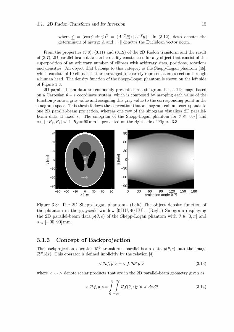
From the properties (3.8), (3.11) and (3.12) of the 2D Radon transform and the resultof (3.7), 2D parallel-beam data can be readily constructed for any object that consist of thesuperposition of an arbitrary number of ellipses with arbitrary sizes, positions, rotationsand densities. An object that belongs to this category is the Shepp-Logan phantom [46],which consists of 10 ellipses that are arranged to coarsely represent a cross-section througha human head. The density function of the Shepp-Logan phantom is shown on the left sideof Figure 3.3.
2D parallel-beam data are commonly presented in a sinogram, i.e., a 2D image basedon a Cartesian θ − s coordinate system, which is composed by mapping each value of thefunction p onto a gray value and assigning this gray value to the corresponding point in thesinogram space. This thesis follows the convention that a sinogram column corresponds toone 2D parallel-beam projection, whereas one row of the sinogram visualizes 2D parallel-beam data at fixed s. The sinogram of the Shepp-Logan phantom for θ ∈ [0, π] ands ∈ [−Ro, Ro] with Ro = 90 mm is presented on the right side of Figure 3.3.
x [mm]
y [m
m]
−90 −60 −30 0 30 60 90
−90
−60
−30
0
30
60
90
projection angle θ [°]
s [m
m]
0 30 60 90 120 150 180
−90
−60
−30
0
30
60
90
Figure 3.3: The 2D Shepp-Logan phantom. (Left) The object density function ofthe phantom in the grayscale window [0 HU, 40 HU]. (Right) Sinogram displayingthe 2D parallel-beam data p(θ, s) of the Shepp-Logan phantom with θ ∈ [0, π] ands ∈ [−90, 90] mm.
3.1.3 Concept of Backprojection
The backprojection operator R# transforms parallel-beam data p(θ, s) into the imageR#p(x). This operator is defined implicitly by the relation [4]
< Rf, p >=< f,R#p > (3.13)
where < ·, · > denote scalar products that are in the 2D parallel-beam geometry given as
< Rf, p >=
π∫
0
∞∫
−∞Rf(θ, s)p(θ, s) ds dθ (3.14)
16 Chapter 3. Classical Theory for Image Reconstruction in Two Dimensions
and< f,R#p >=
∫∫
R2
f(x)R#p(x) dx. (3.15)
Using the definition of the 2D Radon transform (3.3) in (3.14) and applying the change ofvariable x = sθ + tθ⊥ of Jacobian 1 yields
< Rf, p > =
π∫
0
∞∫
−∞
∞∫
−∞f(sθ + tθ⊥) dt p(θ, s) ds dθ
=
π∫
0
∫∫
R2
f(x)p(θ, x · θ) dx dθ.
(3.16)
Changing the order of integration in (3.16) and using the definitions (3.13) and (3.15) resultsin
R#p(x) =
π∫
0
p(θ, θ · x) dθ, (3.17)
which is the wanted expression for the backprojection operator.In order to obtain a valid backprojection result at a point x according to (3.17), 2D
parallel-beam data need to be known for all θ ∈ [0, π) and within each parallel-beamprojection at s = x · θ. The computation of R#p(x) thus requires integral data associatedto all lines that contain x. On the other hand, if 2D parallel-beam data are known forθ ∈ [0, π] and s ∈ [−Ro, Ro], the function R#p can be computed everywhere in the imageplane.
x [mm]
y [m
m]
−90 −60 −30 0 30 60 90
−90
−60
−30
0
30
60
90
x [mm]
y [m
m]
−90 −60 −30 0 30 60 90
−90
−60
−30
0
30
60
90
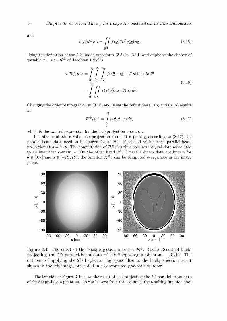
Figure 3.4: The effect of the backprojection operator R#. (Left) Result of back-projecting the 2D parallel-beam data of the Shepp-Logan phantom. (Right) Theoutcome of applying the 2D Laplacian high-pass filter to the backprojection resultshown in the left image, presented in a compressed grayscale window.
The left side of Figure 3.4 shows the result of backprojecting the 2D parallel-beam dataof the Shepp-Logan phantom. As can be seen from this example, the resulting function does
3.1. 2D Radon Transform and Its Inversion 17
not correspond to the object density f . However, the following relation can be established[46]:
R#Rf(x) =
π∫
0
Rf(θ, θ · x) dθ =
π∫
0
∞∫
−∞f
((θ · x)θ + tθ⊥
)dt dθ
=
π∫
0
∞∫
−∞f(x + tθ⊥) dt dθ =
∫∫
R2
1‖x− x′‖f(x′) dx′.
(3.18)
Hence, R#Rf corresponds to the result of convolving f with the 2D low-pass filter kernel1/‖x‖. Discontinuities in the object density function f can be determined by applyingthe 2D Laplacian operator on R#Rf [4], see the right side of Figure 3.4. This approach,however, does not allow a quantitative recovery of the object density.
3.1.4 Classical Inversion Formula for the 2D Radon Trans-form
In the following, an inverse of the 2D Radon transform operator is derived. This result isbased on a link between the 2D Fourier transform in x of the object density function andthe 1D Fourier transform in s of the 2D parallel-beam data at projection angle θ. TheseFourier transforms are given respectively as [46]
Fxf(ξ) =∫∫
R2
f(x)e−2πiξ·x dx and FsRf(θ, σ) =
∞∫
−∞Rf(θ, s)e−2πiσs ds (3.19)
with the subscript parameter denoting the argument in which the transform is applied.The link between these two functions, which is known as the 2D Fourier slice theorem, isobtained as
FsRf(θ, σ) =
∞∫
−∞Rf(θ, s)e−2πiσs ds
=
∞∫
−∞
∞∫
−∞f(sθ + tθ⊥)e−2πiσs dt ds
=∫∫
R2
f(x)e−2πiσθ·x dx
= Fxf(σθ).
(3.20)
The inversion formula for the 2D Radon transform is now derived in a similar fashionas in [4] by first expressing the object as the inverse 2D Fourier transform of Fxf , i.e., as
f(x) =∫∫
R2
Fxf(ξ)e2πiξ·x dξ (3.21)
with ξ = (ξ1, ξ2)T. The change of variable from Cartesian to polar coordinates
ξ1 = σ cos θ, ξ2 = σ sin θ (3.22)
18 Chapter 3. Classical Theory for Image Reconstruction in Two Dimensions
of Jacobian |σ| and the use of the 2D Fourier slice theorem (3.20) transforms (3.21) into
f(x) =
π∫
0
∞∫
−∞|σ|Fxf(σθ)e2πiσθ·x dσ dθ
=
π∫
0
∞∫
−∞|σ|FsRf(θ, σ)e2πiσθ·x dσ dθ
(3.23)
and thus into an analytical inversion approach for the 2D Radon transform, which is basedon the following steps:
Step 1 – 1D Filtering: 2D parallel-beam data at fixed θ are filtered in s to obtain
pF (θ, s) =
∞∫
−∞Fshramp(σ)Fsp(θ, σ)e2πiσs dσ (3.24)
=
Ro∫
−Ro
hramp(s− s′)p(θ, s) ds′ (3.25)
with the filter kernel hramp defined in frequency and spatial domain, respectively, as
Fshramp(σ) = |σ| and hramp(s) = limb→∞
b∫
−b
|σ|e2πiσsdσ. (3.26)
The function hramp is of infinite support and known as the ramp filter kernel [46].Note that the limits of integration in (3.25) were adjusted to−Ro and Ro, respectively,and that this adjustment became possible because of the bounded support of p.
Step 2 – 2D Backprojection: Backprojection of the filtered parallel-beam projectionsonto the image plane using the operator R# yields the object density function as
f(x) =
π∫
0
pF (θ, x · θ) dθ. (3.27)
The analytical filtered backprojection (FBP) inversion method presented in (3.25)-(3.27) isreferred to as the classical 2D Radon inversion method from now on. For a valid recoveryof the value of f at a single point x, this method requires filtered parallel-beam data pF
to be known for all projection angles θ ∈ [0, π), using in every projection the sample atx · θ. On the other hand, the values pF at any fixed angle θ can only be computed if thecorresponding parallel-beam projection is non-truncated, because the convolution equation(3.25) corresponds to a global filter operation. In order to allow object density to berecovered at a single point, the 2D Radon inversion formula thus requires non-truncatedprojections for θ ∈ [0, π), or, in other words, the integral data associated to every lineintersecting the object. Note that if recovery of f according to (3.25)-(3.27) can be achievedat some point x, then it is achievable everywhere within Ωf .
3.1. 2D Radon Transform and Its Inversion 19
3.1.5 Parallel Beam Reconstruction Formula for RedundantData
In the previous section, an inversion formula for the operatorR was given that requires non-truncated parallel-beam data for θ ∈ [0, π]. If p is, for instance, known over an interval θ ∈[0, θmax] with π < θmax < 2π, however, the 2D parallel-beam data contains redundancies.That means that data samples at coordinates (θ, s) and at (θ + π,−s) are identical, whichfollows from (3.10); see Figure 3.5 for illustration.
0 30 60 90 120 150 180 210 240 270
−90
−60
−30
0
30
60
90
projection angle θ [°]
s [m
m]
A
A
B
BC
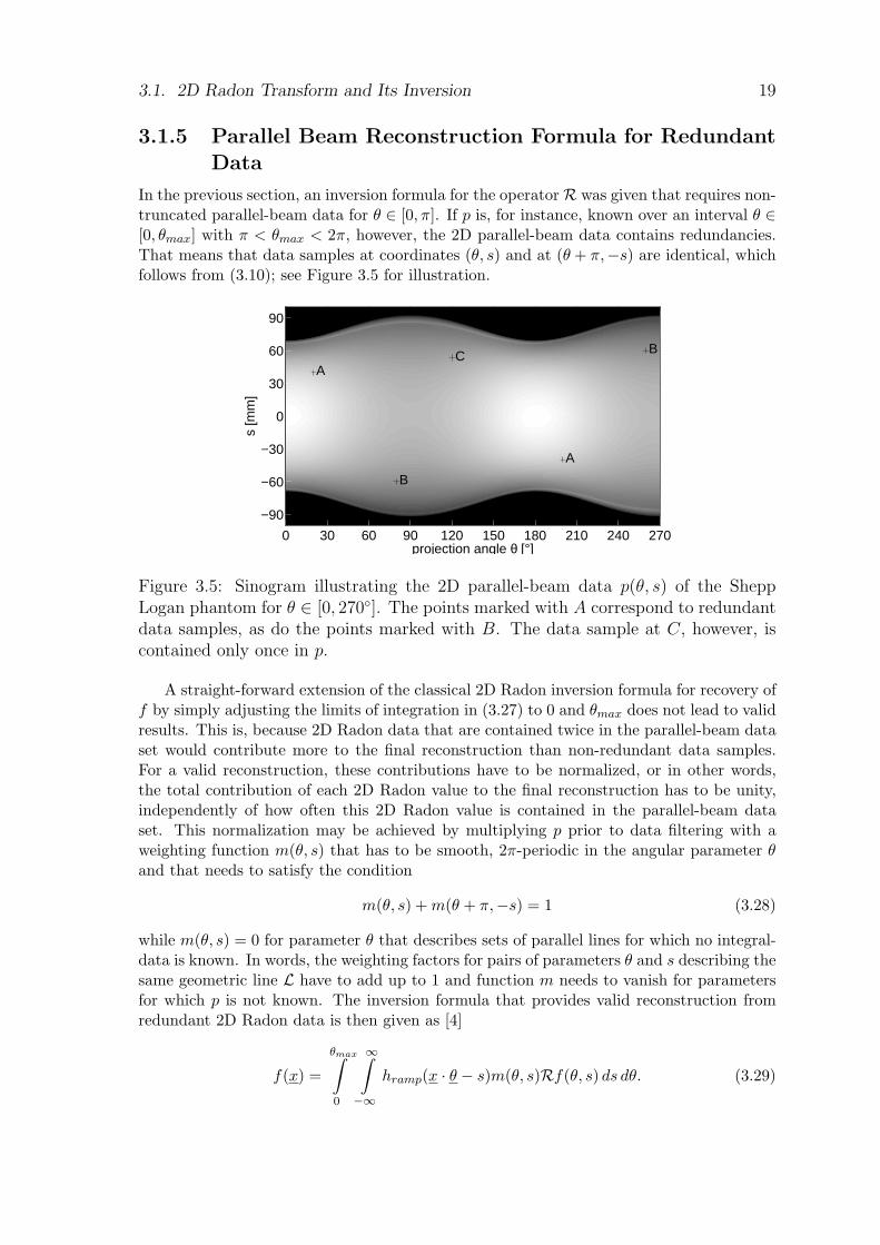
Figure 3.5: Sinogram illustrating the 2D parallel-beam data p(θ, s) of the SheppLogan phantom for θ ∈ [0, 270]. The points marked with A correspond to redundantdata samples, as do the points marked with B. The data sample at C, however, iscontained only once in p.
A straight-forward extension of the classical 2D Radon inversion formula for recovery off by simply adjusting the limits of integration in (3.27) to 0 and θmax does not lead to validresults. This is, because 2D Radon data that are contained twice in the parallel-beam dataset would contribute more to the final reconstruction than non-redundant data samples.For a valid reconstruction, these contributions have to be normalized, or in other words,the total contribution of each 2D Radon value to the final reconstruction has to be unity,independently of how often this 2D Radon value is contained in the parallel-beam dataset. This normalization may be achieved by multiplying p prior to data filtering with aweighting function m(θ, s) that has to be smooth, 2π-periodic in the angular parameter θand that needs to satisfy the condition
m(θ, s) + m(θ + π,−s) = 1 (3.28)
while m(θ, s) = 0 for parameter θ that describes sets of parallel lines for which no integral-data is known. In words, the weighting factors for pairs of parameters θ and s describing thesame geometric line L have to add up to 1 and function m needs to vanish for parametersfor which p is not known. The inversion formula that provides valid reconstruction fromredundant 2D Radon data is then given as [4]
f(x) =
θmax∫
0
∞∫
−∞hramp(x · θ − s)m(θ, s)Rf(θ, s) ds dθ. (3.29)
20 Chapter 3. Classical Theory for Image Reconstruction in Two Dimensions
A common additional constraint in this context is to require that m(θ, s) ≥ 0 so that eachmeasured data sample has positive contribution to the final reconstruction.
3.1.6 Numerical Reconstruction Algorithm
In the practical context of 2D CT, reconstruction of object density is usually carried outfrom sampled 2D parallel-beam data. CT scanners of the first generation [71, 48], forinstance, consisted of an X-ray source and one detector element and therefore acquired onemeasurement ray, i.e. one sample of p, at a time. During the scan, the source-detectorassembly was translated and rotated, which allowed function p to be determined within thedesired intervals in θ and s, but only at a finite number of sampling positions dependingon the increments of the scanner motion. This section presents a numerical FBP algorithmbased on the results of Section 3.1.4 to compute from the discrete 2D parallel-beam dataan estimate of the true object density. This estimate will be denoted as fe where thesuperscript e emphasizes that the entity is computed from sampled data. For convenience,but without loss of generality, we assume that the sampling in both s and θ is uniform withdiscretization steps given as ∆s and ∆θ, respectively.
−10 −5 0 5 10
−0.5
0
0.5
1
s [mm]
h ram
p(s)
Figure 3.6: The ramp filter hbramp with rectangular band-limitation, presented in
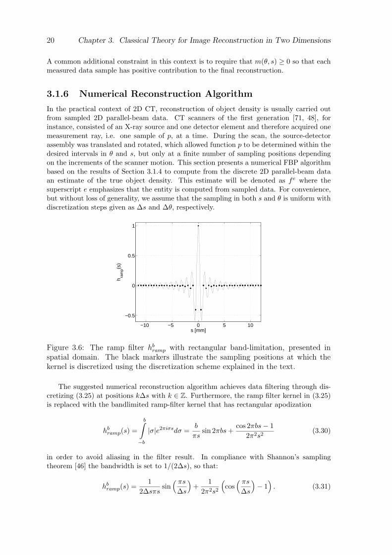
spatial domain. The black markers illustrate the sampling positions at which thekernel is discretized using the discretization scheme explained in the text.
The suggested numerical reconstruction algorithm achieves data filtering through dis-cretizing (3.25) at positions k∆s with k ∈ Z. Furthermore, the ramp filter kernel in (3.25)is replaced with the bandlimited ramp-filter kernel that has rectangular apodization
hbramp(s) =
b∫
−b
|σ|e2πiσsdσ =b
πssin 2πbs +
cos 2πbs− 12π2s2
(3.30)
in order to avoid aliasing in the filter result. In compliance with Shannon’s samplingtheorem [46] the bandwidth is set to 1/(2∆s), so that:
hbramp(s) =
12∆sπs
sin( πs
∆s
)+
12π2s2
(cos
( πs
∆s
)− 1
). (3.31)
3.1. 2D Radon Transform and Its Inversion 21
Figure 3.6 shows the filter kernel hbramp with the positions where this kernel is evaluated
using the suggested discretization scheme. For improved computational efficiency, the 1Dconvolution in (3.25) is carried out using standard signal processing techniques, i.e., usingmultiplication in frequency domain and using the fast-Fourier transform (FFT) and theinverse FFT to convert between the domains.
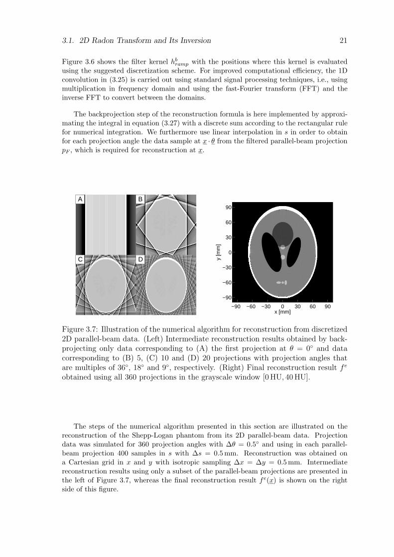
The backprojection step of the reconstruction formula is here implemented by approxi-mating the integral in equation (3.27) with a discrete sum according to the rectangular rulefor numerical integration. We furthermore use linear interpolation in s in order to obtainfor each projection angle the data sample at x · θ from the filtered parallel-beam projectionpF , which is required for reconstruction at x.
C
A
D
B
x [mm]
y [m
m]
−90 −60 −30 0 30 60 90
−90
−60
−30
0
30
60
90
Figure 3.7: Illustration of the numerical algorithm for reconstruction from discretized2D parallel-beam data. (Left) Intermediate reconstruction results obtained by back-projecting only data corresponding to (A) the first projection at θ = 0 and datacorresponding to (B) 5, (C) 10 and (D) 20 projections with projection angles thatare multiples of 36, 18 and 9, respectively. (Right) Final reconstruction result f e
obtained using all 360 projections in the grayscale window [0 HU, 40 HU].
The steps of the numerical algorithm presented in this section are illustrated on thereconstruction of the Shepp-Logan phantom from its 2D parallel-beam data. Projectiondata was simulated for 360 projection angles with ∆θ = 0.5 and using in each parallel-beam projection 400 samples in s with ∆s = 0.5mm. Reconstruction was obtained ona Cartesian grid in x and y with isotropic sampling ∆x = ∆y = 0.5mm. Intermediatereconstruction results using only a subset of the parallel-beam projections are presented inthe left of Figure 3.7, whereas the final reconstruction result fe(x) is shown on the rightside of this figure.
22 Chapter 3. Classical Theory for Image Reconstruction in Two Dimensions
3.2 2D Fan-Beam Transform and Its Classical In-
version Formula
The considerations in the previous section provided a general introduction into the con-cepts of analytical reconstruction theory. Most practical CT scanners used for 2D imaging,however, do not acquire data in the parallel-beam geometry. Data acquisition happens withmeasurement rays that occur in groups of fans on the image plane rather than in parallelsets [47]. This described scenario will here be referred to as the 2D fan-beam geometry,and image reconstruction in this geometry will be discussed below.
3.2.1 The 2D Fan-Beam Geometry
Diagnostic CT scanners may be used to acquire 1D projection data by sending X- rays fromthe X-ray focal spot through the image plane; these rays pass the object and eventuallyinteract with an appropriately located X-ray detector [71, 47]. During the scan, X-ray sourceand detector typically rotate as a single assembly around the object under investigation, sothat projections are acquired with the X-ray focal spot moving along a circular trajectoryon the image plane. The radius of this trajectory will be denoted using the symbol Rand since the source is necessarily located outside the object region Ωf , we have R > Ro.Without loss of generality, it is here assumed that the circular trajectory is centered on theimage plane origin (0, 0)T and that the source is located on the positive x-axis at the startof the scan. The function
a(λ) = (R cosλ,R sinλ)T (3.32)
then gives the source location during acquisition; the trajectory parameter λ correspondsto the source polar angle and may take values λ ∈ [0, λmax] in our geometric set-up.
a
x
y
f
R
max
a
a 0
x
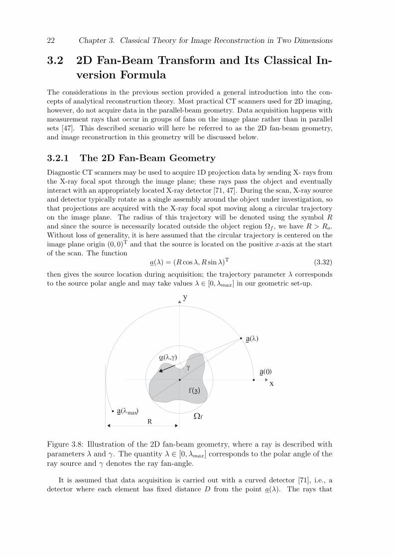
Figure 3.8: Illustration of the 2D fan-beam geometry, where a ray is described withparameters λ and γ. The quantity λ ∈ [0, λmax] corresponds to the polar angle of theray source and γ denotes the ray fan-angle.
It is assumed that data acquisition is carried out with a curved detector [71], i.e., adetector where each element has fixed distance D from the point a(λ). The rays that
3.2. 2D Fan-Beam Transform and Its Classical Inversion Formula 23
connect the source point with all detector elements form a fan and for each such fan, acentral ray can be identified, i.e., the ray that passes through the origin of the image plane(0, 0)T. Each ray within one fan may then be addressed using the fan angle γ ∈ [−γm, γm]that it describes with the central ray, where γ increases in the clockwise direction. Thequantity γm denotes the absolute value of the fan-angle of the ray that intersects with thefirst or last element of the detector, respectively. We assume that the detector is largeenough so that all rays that diverge from the source and intersect the region Ωf also hitthe detector and this condition will be met if γm = asin(Ro/R).
For a description of the 2D fan-beam data let us furthermore introduce the two unitvectors
eu(λ) = (− sinλ, cosλ)T (3.33)ew(λ) = (cosλ, sinλ)T. (3.34)
Note that the vector eu(λ) is tangent to the source trajectory at a(λ) while ew(λ) gives thedirection from the origin (0, 0)T towards the source a(λ). The unit vector along the raydescribed with parameters λ and γ is then given as
α(λ, γ) = sin γ eu(λ)− cos γ ew(λ). (3.35)
3.2.2 The 2D Fan-Beam Transform
According to the data model of section 2, measurements in the fan-beam geometry thenyields samples of the function
g(λ, γ) =
∞∫
0
f (a(λ) + tα(λ, γ)) dt. (3.36)
Function g will be referred to as fan-beam data from now on and fan-beam data at fixed λwill be called a fan-beam projection. Due to the geometric assumptions introduced in theprevious section
g(λ, γ) = 0 for |γ| > γm (3.37)
so that all acquired fan-beam projections are non-truncated.Since a(λ) is always outside the region Ωf , either the ray facing in direction α or the one
facing in direction −α will never intersect the object. Consequently, the limits of integrationin (3.36) can be modified to
g(λ, γ) =
∞∫
−∞f (a(λ) + tα(λ, γ)) dt (3.38)
without changing the fan-beam data function. This modification allows us to establish alink between samples of fan-beam data and 2D Radon data, as described below. A specificselection of parameters λ and γ defines one specific ray, and thus also one specific lineL on the image plane. The unit vectors parallel and orthogonal to this line L are given,respectively, as
θ⊥(λ, γ) = α(λ, γ) and θ(λ, γ) = cos γeu(λ) + sin γew(λ). (3.39)
24 Chapter 3. Classical Theory for Image Reconstruction in Two Dimensions
Following this geometric property and the definition in (3.38), the fan-beam data sampleg(λ, γ) thus coincides with the value of the 2D Radon transform Rf(θ(λ, γ), s(λ, γ)) withthe arguments given as
θ(λ, γ) = λ +π
2− γ and s(λ, γ) = a(λ) · θ(λ, γ) = R sin γ. (3.40)
source polar angle λ [°]
fan
angl
e γ
[°]
−80 −80 −80
−40 −40 −40
0 0 0
40 40 40
80 80 80
10
10
50
50
50
90
90
9013
0
130
130
170
170
170
210
210
0 30 60 90 120 150 180 210−20
−15
−10
−5
0
5
10
15
20
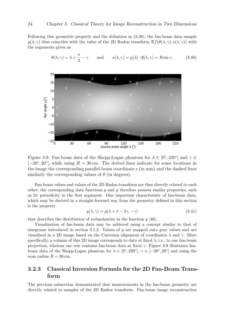
Figure 3.9: Fan-beam data of the Shepp-Logan phantom for λ ∈ [0, 220] and γ ∈[−20, 20], while using R = 30 cm. The dotted lines indicate for some locations inthe image the corresponding parallel-beam coordinate s (in mm) and the dashed linessimilarly the corresponding values of θ (in degrees).
Fan-beam values and values of the 2D Radon transform are thus directly related to eachother; the corresponding data functions p and g therefore possess similar properties, suchas 2π periodicity in the first argument. One important characteristic of fan-beam data,which may be derived in a straight-forward way from the geometry defined in this sectionis the property
g(λ, γ) = g(λ + π − 2γ,−γ) (3.41)
that describes the distribution of redundancies in the function g [46].Visualization of fan-beam data may be achieved using a concept similar to that of
sinograms introduced in section 3.1.2. Values of g are mapped onto gray values and arevisualized in a 2D image based on the Cartesian alignment of coordinates λ and γ. Morespecifically, a column of this 2D image corresponds to data at fixed λ, i.e., to one fan-beamprojection, whereas one row contains fan-beam data at fixed γ. Figure 3.9 illustrates fan-beam data of the Shepp-Logan phantom for λ ∈ [0, 220], γ ∈ [−20, 20] and using thescan radius R = 30 cm.
3.2.3 Classical Inversion Formula for the 2D Fan-Beam Trans-form
The previous subsection demonstrated that measurements in the fan-beam geometry aredirectly related to samples of the 2D Radon transform. Fan-beam image reconstruction
3.2. 2D Fan-Beam Transform and Its Classical Inversion Formula 25
may thus be achieved by a rather straight-forward application of techniques derived insection 3.1.4. It can be shown that using the 2D Radon inversion formula for redundantdata (presented in section 3.1.5) and applying the change of variables (θ, s) → (λ, γ), whichhas been defined in (3.40), directly leads to the following analytical inversion formula forthe 2D fan-beam geometry [4, 46]:
f(x) =
λmax∫
0
R
‖x− a(λ)‖2
π/2∫
−π/2
hramp (sin(γ∗(x)− γ)) cos γ m(λ, γ) g(λ, γ) dγ dλ. (3.42)
The quantity
γ∗(x) = atan(
x · eu(λ)R− x · ew(λ)
)(3.43)
in this formula denotes the fan angle of the measurement ray that diverges from a(λ) andcontains x, the function hramp is the ramp filter kernel and m is a redundancy weightingfunction. Note that here and in the following, the superscript ∗ is used to denote a functionthat depends on λ, without explicitly listing this argument.
The redundancy weight m in (3.42) is similar to the function m in the 2D parallel-beamgeometry: it equalizes the contribution of every 2D Radon value contained in the set offan-beam data for the final reconstruction. Function m needs to be smooth in γ [46], 2π-periodic in λ and is assumed to be 0 at parameters λ for which no ray-integrals have beenmeasured. Equalization will then be achieved if m satisfies the normalization condition
m(λ, γ) + m(λ + π − 2γ,−γ) = 1, (3.44)
which follows directly from the redundancy property (3.41) of the fan-beam data function.Equation 3.42 will be referred to as the classical analytical fan-beam inversion formula
throughout this thesis. It has FBP structure and may be decomposed into the followingthree steps:
Step 1 – Data Weighting: Fan-beam data are multiplied with the redundancy weight-ing function and a cosine term to yield weighted fan-beam projections
gW (λ, γ) = m(λ, γ) cos γ g(λ, γ). (3.45)
Step 2 – 1D Filtering: The weighted fan-beam projections are filtered in γ using thekernel of the ramp filter to obtain filtered projections
gF (λ, γ) =
γm∫
−γm
hramp(sin(γ − γ′))gW (λ, γ′)dγ′. (3.46)
Step 3 – 2D Weighted Backprojection: The function gF is backprojected onto theimage plane using a weighting factor that is inversely proportional to the square ofthe distance between the source position a(λ) and the point x where reconstructionis to be achieved to obtain
f(x) =
λmax∫
0
R
‖x− a(λ)‖2gF (λ, γ∗(x)) dλ (3.47)
with the function γ∗ defined in (3.43).
26 Chapter 3. Classical Theory for Image Reconstruction in Two Dimensions
In order to obtain valid reconstruction of f at any point x ∈ Ωf using the classicalscheme described above, we require filtered fan-beam projections for a scan with at leastλmax = π + 2γm [46, 47], which is referred to as a short-scan. Note also that data filteringat any λ can only be achieved if the corresponding projection is non-truncated, which isguaranteed when g(λ, γ) is known over the interval γ ∈ [−γm, γm]. The redundancy weightused for reconstruction can be selected somewhat flexibly within the constraints imposedby the normalization and the smoothness conditions. One possible explicit espression forfunction m can, for instance, be given as 1
m(λ, γ) =
sin2(
π4 · λ
γthres+γ
)if 0 ≤ λ < 2(γthres + γ),
1 if 2(γthres + γ) ≤ λ < π + 2γ,
sin2(
π4 · π+2γthres−λ
γthres+γ
)if π + 2γ ≤ λ < π + 2γthres,
0 if π + 2γthres ≤ λ < 2π.
(3.48)
The weighting function defined in this equation gives a contribution of 1 to each ray integralthat is measured only once and nicely balances the contributions of redundant data samples,using the property of the trigonometric functions, so that the weights corresponding to datasamples considered twice for reconstruction sum up to unity.
source polar angle λ [°]
fan
angl
e γ
[°]
0.1
0.1
0.1
0.1
0.1
0.3
0.3
0.3
0.3
0.3
0.3
0.5
0.5
0.5
0.5
0.5
0.50.7
0.7
0.7
0.7
0.7
0.70.9
0.9
0.9
0.9
0.9
0.9
0 30 60 90 120 150 180 210−20
−15
−10
−5
0
5
10
15
20
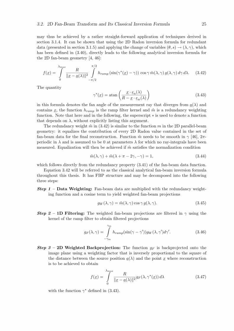
Figure 3.10: Illustration of the Parker weighting function which is used to accountfor data redundancies in fan-beam data g.
The parameter γthres in (3.48), which may here take values γm ≤ γthres ≤ π/2, providessome control about the amount of data used for reconstruction. For γthres = γm, equation(3.48) corresponds to the redundancy weighting function suggested by Parker [75], whichis widely used for fan-beam reconstruction from a short-scan trajectory, i.e., for λmax =π + 2γm. Figure 3.10 illustrates the Parker weighting function for γm = 20. For the casethat fan-beam projections are acquired over an interval in λ exceeding a short-scan, the useof γthres = (λmax−π)/2 was suggested [79], so that all known values of g receive a non-zerocontribution to the final reconstruction; the resulting weighting function will be referred toas the generalized Parker weight from now on.
1Note that in the equation, we only define one period of the redundancy weighting function,which is 2π periodic in λ.
3.2. 2D Fan-Beam Transform and Its Classical Inversion Formula 27
3.2.4 Numerical Reconstruction Algorithm
From the results of section 3.2.3, a numerical algorithm may be given for image reconstruc-tion from fan-beam data in practical CT applications. CT data acquisition allows in generalthe function g to be determined only at a finite number of sampling positions. Here it isassumed that the polar angles λ of the source of two adjacent fan-beam projections differ bythe fixed increment ∆λ and that furthermore the rays within one fan-beam projection areuniformly sampled in γ; the angular sample spacing between two adjacent rays is denotedas ∆γ. This section presents a numerical algorithm to compute from this sampled fan-beamdata function an estimate of the object density. This estimate will be denoted as fe.
C
A
D
B
x [mm]
y [m
m]
−90 −60 −30 0 30 60 90
−90
−60
−30
0
30
60
90
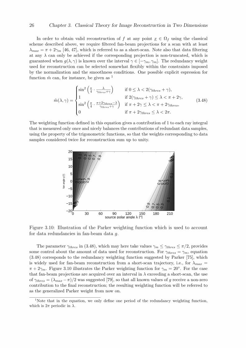
Figure 3.11: Illustration of the numerical 2D fan-beam reconstruction algorithm.(Left) Intermediate results obtained by backprojecting only (A) 1 (B) 5 (C) 10 or(D) 20 filtered fan-beam projections, respectively, which are evenly distributed overthe known interval [0, 220]. (Right) Final reconstruction result f e obtained using440 fan-beam projections, presented in the grayscale window [0 HU, 40 HU].
The numerical algorithm achieves data filtering by first modifying (3.46) using theidentity [46]
hramp (sin(γ∗(x)− γ)) = hramp
(γ∗(x)− γ
γ∗(x)− γsin(γ∗(x)− γ))
)
=(
γ∗(x)− γ
sin(γ∗(x)− γ)
)2
hramp(γ∗(x)− γ)
= hramp(γ∗(x)− γ)
(3.49)
that can be derived using the scaling property of the ramp filter kernel:
hramp(as) =
∞∫
−∞|σ|e2πiσas dσ =
∞∫
−∞
1a2|σ′|e2πiσ′s dσ′
=1a2
hramp(s)
(3.50)
28 Chapter 3. Classical Theory for Image Reconstruction in Two Dimensions
that holds for any a 6= 0. Equation (3.49) then enables us to express the data filteringequation as a 1D convolution in γ of the weighted fan-beam data with the modified rampfilter
hγramp(γ) =
(γ
sin γ
)2
hramp(γ) (3.51)
In our implementation, the function hramp(γ) in (3.51) was substituted with its band-limited version using bandwidth 1/(2∆γ); see section 3.1.6 for details. The resulting filterequation is discretized at the sampling positions k∆γ with k ∈ Z and 1D convolution isagain efficiently carried out by multiplication of the involved functions in frequency domain;see again section 3.1.6. Backprojection is achieved by discretizing (3.47) and using linearinterpolation in γ to obtain in each filtered fan-beam projection the value at the requiredsampling position γ∗(x).
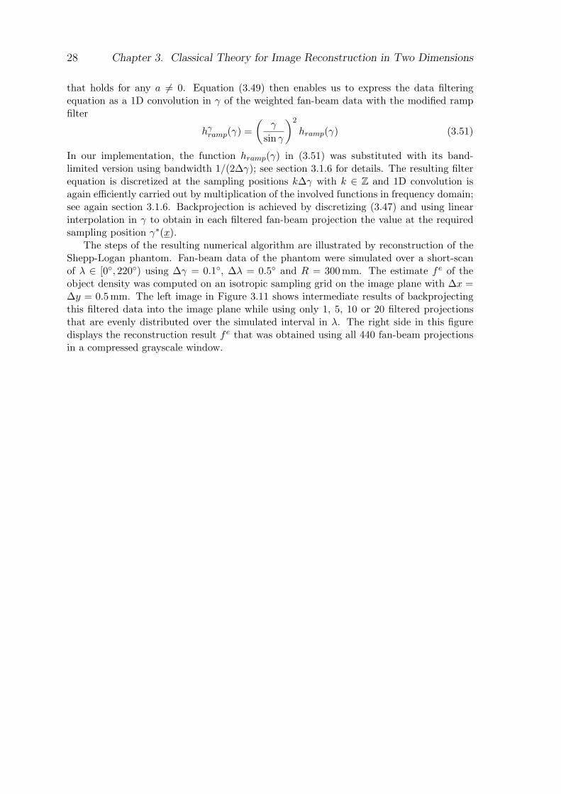
The steps of the resulting numerical algorithm are illustrated by reconstruction of theShepp-Logan phantom. Fan-beam data of the phantom were simulated over a short-scanof λ ∈ [0, 220) using ∆γ = 0.1, ∆λ = 0.5 and R = 300 mm. The estimate fe of theobject density was computed on an isotropic sampling grid on the image plane with ∆x =∆y = 0.5mm. The left image in Figure 3.11 shows intermediate results of backprojectingthis filtered data into the image plane while using only 1, 5, 10 or 20 filtered projectionsthat are evenly distributed over the simulated interval in λ. The right side in this figuredisplays the reconstruction result fe that was obtained using all 440 fan-beam projectionsin a compressed grayscale window.
Chapter 4
Fan-Beam Reconstruction withoutBackprojection Weight
4.1 Introduction
Filtered-backprojection is a common way to achieve image reconstruction in 2D X-ray CT,see, for instance, the classical inversion methods for the 2D parallel beam geometry and 2Dfan beam geometry, as explained in sections 3.1.4 and 3.2.3, respectively.
This chapter addresses the issue of FBP image reconstruction from fan-beam data. Fan-beam reconstruction may be carried out directly, by applying the FBP in the measurementgeometry, see chapter 3.2.3 or the methods in [7, 14, 46, 56, 66, 74], but also indirectly, byfirst rebinning the 2D fan-beam data into the 2D parallel-beam geometry and then using a2D parallel- beam reconstruction method to recover the object density function [10, 46, 73].
Both approaches, direct and indirect, have their pros and cons, and are currently inuse in medical CT scanners. One drawback of indirect approaches is that the rebinningstep comes with additional computational cost. Furthermore, rebinning requires in generalinterpolation in order to yield 2D parallel-beam data with a sampling beneficial for theapplication of a 2D parallel-beam reconstruction method; this interpolation is expected tohave negative impact on the spatial resolution achievable in the reconstruction result.
On the other hand, one disadvantage of the direct FBP approach is that the backpro-jection step includes a weighting factor that varies with both, the source polar angle λ andthe point x where reconstruction is to be performed. This weighting factor is often seenas a source of noise increase [96], and also makes backprojection in the direct approachmore computationally demanding and more difficult to code in hardware than the indirectapproach [10, 73].
This chapter is focussed on the direct FBP approach and presents a novel FBP formulafor image reconstruction from 2D fan-beam data collected over a full 2π scan, which isderived from the alternative inversion formula for fan-beam data suggested by Noo et al.[66]. Our novel formula operates directly in the fan-beam geometry, so that it does notrequire any data rebinning, and it also comes along without the spatially varying weightingfactor during backprojection.
29
30 Chapter 4. Fan-Beam Reconstruction without Backprojection Weight
4.2 Alternative Inversion Formula for the 2D Fan-
Beam Transform
In [66], Noo et al. suggested a direct fan-beam inversion formula that is different from theclassical approach introduced in section 3.2.3. Noo’s alternative formula is based on theclassical 2D parallel beam inversion method
f(x) =
π∫
0
pF (θ, θ · x) dθ with pF (θ, s) =
∞∫
−∞hramp(s− s′)p(θ, s′) ds′ (4.1)
and derived using the following two concepts:
Concept 1 - Decomposition of the ramp filter hramp :
In Fourier domain, the ramp filter may be developed into
Fshramp(σ) = |σ| = σ signσ =12π
(−i)signσ 2πiσ
=12πFshhilb(σ)Fshder(σ)
(4.2)
where hder and hhilb denote the kernels of the differentiation operator and of theHilbert transform, respectively, which are given as
hder(s) =
∞∫
−∞2πiσ e2πiσs dσ (4.3)
and
hhilb(s) =
∞∫
−∞(−i) signσ e2πiσsdσ. (4.4)
Hence, ramp filtering of a 1D function may be alternatively achieved by applyingsubsequently but in arbitrary order the following operations: data differentiation,convolution with the kernel of the Hilbert transform and data weighting. The filteringin (4.1) can thus be expressed as
pF (θ, s) =12π
∂
∂spH(θ, s) (4.5)
with pH(θ, s) denoting the Hilbert transform of 2D parallel beam data in the param-eter s:
pH(θ, s) =
∞∫
−∞hhilb(s− s′)p(θ, s′) ds′. (4.6)
Hence, an alternative expression of the 2D parallel beam inversion formula (4.1) isgiven as
f(x) =12π
π∫
0
∂
∂spH(θ, s)
∣∣∣∣s=x·θ
dθ. (4.7)
4.2. Alternative Inversion Formula for the 2D Fan-Beam Transform 31
Concept 2 - Hilbert transform in angular parameter γ :
Image reconstruction according to (4.7) requires values of the function pH , whichmay be obtained according to (4.6). However, as shown in [66], samples of pH mayalso be obtained directly in the fan-beam geometry, namely by using the convolution
pH(θ, a(λ) · θ) =
π∫
−π
hhilb(sin(θ − γ)) g(λ, γ) dγ. (4.8)
In order to proof the identity in (4.8), we use the fact that sin(θ−γ) = −α(λ, γ)·θ withα(λ, γ) defined in (3.35), which follows directly from the theorems of trigonometricfunctions, and develop the right hand side in (4.8) as
π∫
−π
hhilb(sin(θ − γ)) g(λ, γ) dγ =
π∫
−π
hhilb(−α(λ, γ) · θ) g(λ, γ) dγ
=
π∫
−π
hhilb(−α(λ, γ) · θ)∞∫
0
f(a(λ) + tα(λ, γ)) dt dγ
=
π∫
−π
∞∫
0
t hhilb(−tα(λ, γ) · θ)f(a(λ) + tα(λ, γ)) dt dγ
=∫∫
R2
hhilb((a(λ)− x) · θ)f(x) dx
=∫∫
R2
∞∫
−∞δ(s− x · θ) hhilb(a(λ) · θ − s)f(x) ds dx
=
∞∫
−∞hhilb(a(λ) · θ − s) p(θ, s) ds = pH(θ, a(λ) · θ).
(4.9)
The step from line 2 to line 3 in this derivation involves the scaling property of theHilbert kernel, namely the identity t hhilb(ts) = hhilb(s) for t 6= 0, which can bederived analog to the scheme in (3.50). Furthermore, to obtain line 4 from line 3,we use the change of variable x = a(λ) + tα(λ, γ), which comes with a Jacobian thatcancels out the factor t in front of the expression of the Hilbert kernel function. Notethat the calculation of the value pH(θ, s) according to (4.8) requires a non-truncatedfan-beam projection with the source at polar angle λ that satisfies a(λ) · θ = s.Geometrically, we thus require integral data associated to all rays that diverge froma(λ) and that intersect Ωf . Requirement on the data is therefore different from thatof the conventional filter equation (4.6), which requires integral data to be known forall lines that are orthogonal to θ and that intersect Ωf .
Using the two concepts listed above, Noo et al. derived an alternative direct FBPformula for reconstruction from fan-beam data g(λ, γ). For a full-length derivation of thisformula, we direct the reader to [66]. Reconstruction from full-scan fan-beam data usingNoo’s alternative formula is achieved as
f(x) =12π
2π∫
0
w(λ, x)‖x− a(λ)‖
γm∫
−γm
hhilb(sin(γ∗(x)− γ)) g(λ, γ) dγ dλ (4.10)
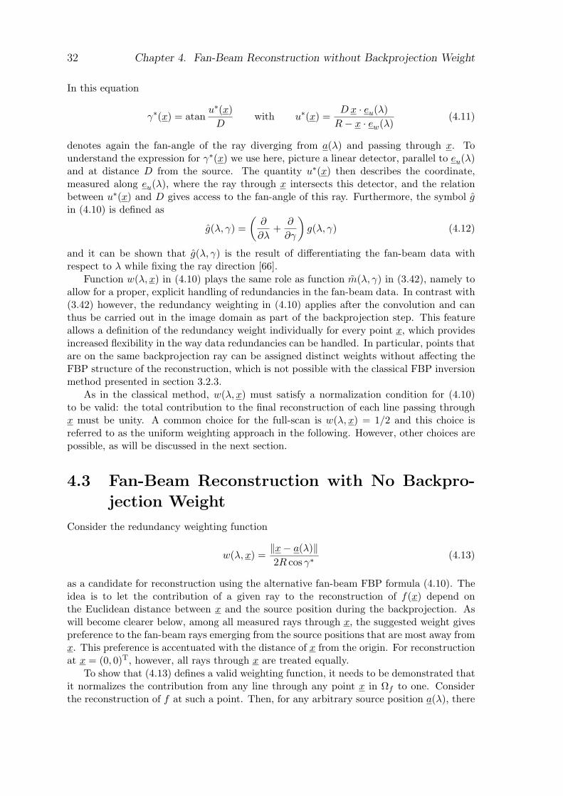
32 Chapter 4. Fan-Beam Reconstruction without Backprojection Weight
In this equation
γ∗(x) = atanu∗(x)
Dwith u∗(x) =
D x · eu(λ)R− x · ew(λ)
(4.11)
denotes again the fan-angle of the ray diverging from a(λ) and passing through x. Tounderstand the expression for γ∗(x) we use here, picture a linear detector, parallel to eu(λ)and at distance D from the source. The quantity u∗(x) then describes the coordinate,measured along eu(λ), where the ray through x intersects this detector, and the relationbetween u∗(x) and D gives access to the fan-angle of this ray. Furthermore, the symbol gin (4.10) is defined as
g(λ, γ) =(
∂
∂λ+
∂
∂γ
)g(λ, γ) (4.12)
and it can be shown that g(λ, γ) is the result of differentiating the fan-beam data withrespect to λ while fixing the ray direction [66].
Function w(λ, x) in (4.10) plays the same role as function m(λ, γ) in (3.42), namely toallow for a proper, explicit handling of redundancies in the fan-beam data. In contrast with(3.42) however, the redundancy weighting in (4.10) applies after the convolution and canthus be carried out in the image domain as part of the backprojection step. This featureallows a definition of the redundancy weight individually for every point x, which providesincreased flexibility in the way data redundancies can be handled. In particular, points thatare on the same backprojection ray can be assigned distinct weights without affecting theFBP structure of the reconstruction, which is not possible with the classical FBP inversionmethod presented in section 3.2.3.
As in the classical method, w(λ, x) must satisfy a normalization condition for (4.10)to be valid: the total contribution to the final reconstruction of each line passing throughx must be unity. A common choice for the full-scan is w(λ, x) = 1/2 and this choice isreferred to as the uniform weighting approach in the following. However, other choices arepossible, as will be discussed in the next section.
4.3 Fan-Beam Reconstruction with No Backpro-
jection Weight
Consider the redundancy weighting function
w(λ, x) =‖x− a(λ)‖2R cos γ∗
(4.13)
as a candidate for reconstruction using the alternative fan-beam FBP formula (4.10). Theidea is to let the contribution of a given ray to the reconstruction of f(x) depend onthe Euclidean distance between x and the source position during the backprojection. Aswill become clearer below, among all measured rays through x, the suggested weight givespreference to the fan-beam rays emerging from the source positions that are most away fromx. This preference is accentuated with the distance of x from the origin. For reconstructionat x = (0, 0)T, however, all rays through x are treated equally.
To show that (4.13) defines a valid weighting function, it needs to be demonstrated thatit normalizes the contribution from any line through any point x in Ωf to one. Considerthe reconstruction of f at such a point. Then, for any arbitrary source position a(λ), there
4.3. Fan-Beam Reconstruction with No Backprojection Weight 33
Figure 4.1: Geometric illustrations of the redundantly measured line L. The lineintegral corresponding to L is obtained at source parameters λ and λc. The absolutevalue of the fan angle to the line L is identical in both views, λ and λc.
exists a complementary source parameter λc, such that x, a(λ) and a(λc) are collinearand define a line L (see Figure 4.1). The integral along L is acquired twice, at sourceparameters λ and λc, respectively. From equation (4.13) which defines the weight that eachmeasurement on L receives, and from the relation γ∗c = −γ∗ (see Figure 4.1), it can beshown that
‖x− a(λ)‖2R cos γ∗
+‖x− a(λc)‖2R cos γ∗c
=‖x− a(λ)‖+ ‖x− a(λc)‖
2R cos γ∗
=‖a(λc)− a(λ)‖
2R cos γ∗= 1 .
(4.14)
The result in (4.14) proves that the weighting scheme in (4.13) achieves the required nor-malization to unity of the contribution from each line through x. Hence, the function wsuggested in (4.13) defines a valid weighting scheme. Moreover, since w is proportionalto ‖a(λ) − x‖, it cancels out the backprojection weight 1/‖a(λ) − x‖ in the alternativefan-beam FBP inversion formula (4.10). This means that the computationally costly stepof applying the backprojection weight in a direct FBP reconstruction can be avoided. Incompensation, the convolved fan-beam data just needs to be multiplied by 1/(2R cos γ)prior to backprojection. Substituting the suggested weighting function (4.13) into (4.10)yields the novel direct FBP formula for reconstruction from full-scan fan-beam data:
f(x) =1
4πR
2π∫
0
gF (λ, γ∗) dλ (4.15)
where
gF (λ, γ) =1
cos γ
γm∫
−γm
hhilb(sin(γ − γ′)) g(λ, γ′) dγ′ (4.16)
with g given by equation (4.12). This formula has no backprojection weight.
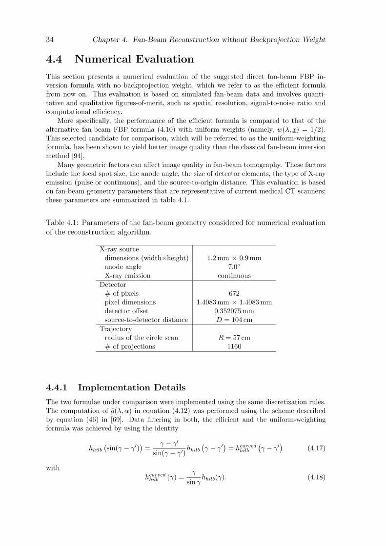
34 Chapter 4. Fan-Beam Reconstruction without Backprojection Weight
4.4 Numerical Evaluation
This section presents a numerical evaluation of the suggested direct fan-beam FBP in-version formula with no backprojection weight, which we refer to as the efficient formulafrom now on. This evaluation is based on simulated fan-beam data and involves quanti-tative and qualitative figures-of-merit, such as spatial resolution, signal-to-noise ratio andcomputational efficiency.
More specifically, the performance of the efficient formula is compared to that of thealternative fan-beam FBP formula (4.10) with uniform weights (namely, w(λ, x) = 1/2).This selected candidate for comparison, which will be referred to as the uniform-weightingformula, has been shown to yield better image quality than the classical fan-beam inversionmethod [94].
Many geometric factors can affect image quality in fan-beam tomography. These factorsinclude the focal spot size, the anode angle, the size of detector elements, the type of X-rayemission (pulse or continuous), and the source-to-origin distance. This evaluation is basedon fan-beam geometry parameters that are representative of current medical CT scanners;these parameters are summarized in table 4.1.
Table 4.1: Parameters of the fan-beam geometry considered for numerical evaluationof the reconstruction algorithm.
X-ray sourcedimensions (width×height) 1.2 mm × 0.9mmanode angle 7.0
X-ray emission continuousDetector
# of pixels 672pixel dimensions 1.4083 mm × 1.4083mmdetector offset 0.352075mmsource-to-detector distance D = 104 cm
Trajectoryradius of the circle scan R = 57 cm# of projections 1160
4.4.1 Implementation Details
The two formulae under comparison were implemented using the same discretization rules.The computation of g(λ, α) in equation (4.12) was performed using the scheme describedby equation (46) in [69]. Data filtering in both, the efficient and the uniform-weightingformula was achieved by using the identity
hhilb
(sin(γ − γ′)
)=
γ − γ′
sin(γ − γ′)hhilb
(γ − γ′
)= hcurved
hilb
(γ − γ′
)(4.17)
withhcurved
hilb (γ) =γ
sin γhhilb(γ). (4.18)
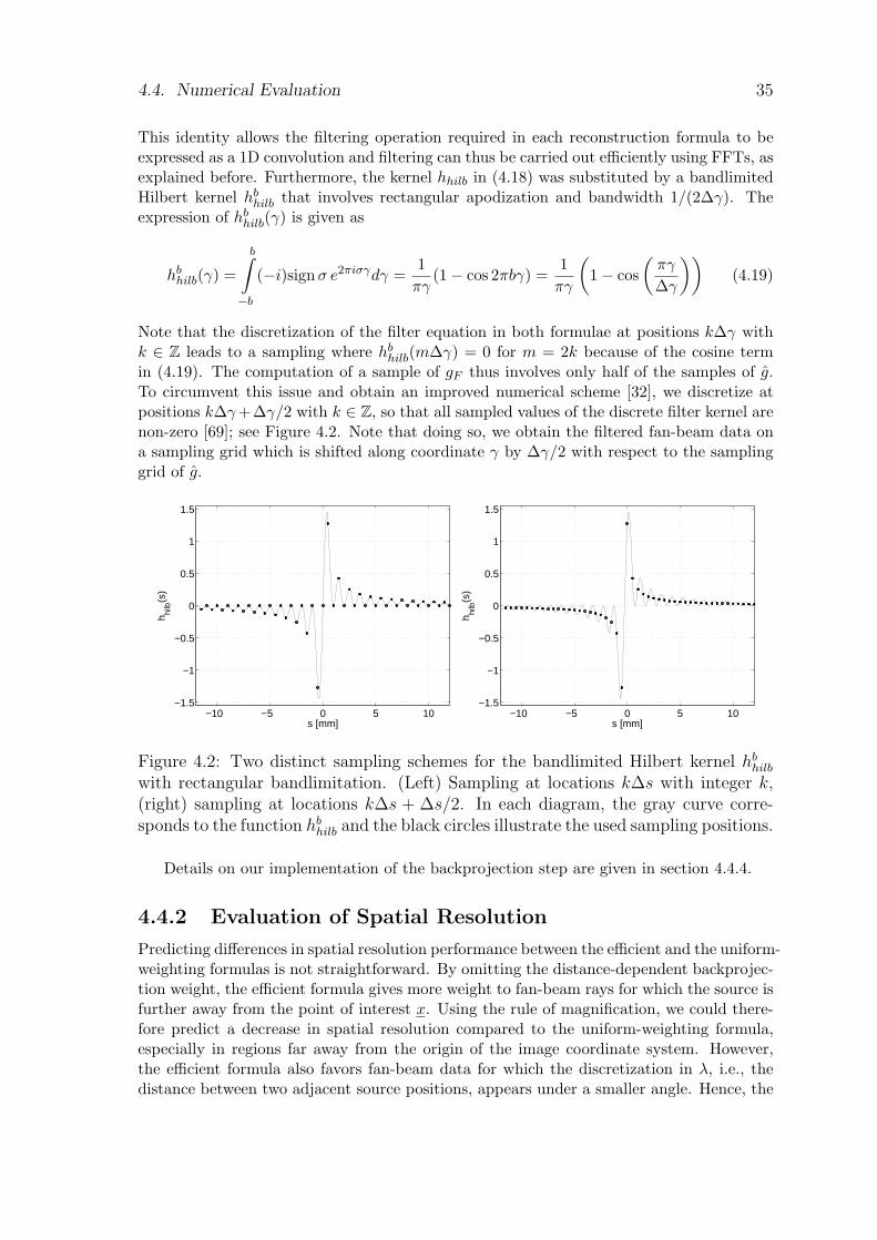
4.4. Numerical Evaluation 35
This identity allows the filtering operation required in each reconstruction formula to beexpressed as a 1D convolution and filtering can thus be carried out efficiently using FFTs, asexplained before. Furthermore, the kernel hhilb in (4.18) was substituted by a bandlimitedHilbert kernel hb
hilb that involves rectangular apodization and bandwidth 1/(2∆γ). Theexpression of hb
hilb(γ) is given as
hbhilb(γ) =
b∫
−b
(−i)sign σ e2πiσγdγ =1
πγ(1− cos 2πbγ) =
1πγ
(1− cos
(πγ
∆γ
))(4.19)
Note that the discretization of the filter equation in both formulae at positions k∆γ withk ∈ Z leads to a sampling where hb
hilb(m∆γ) = 0 for m = 2k because of the cosine termin (4.19). The computation of a sample of gF thus involves only half of the samples of g.To circumvent this issue and obtain an improved numerical scheme [32], we discretize atpositions k∆γ +∆γ/2 with k ∈ Z, so that all sampled values of the discrete filter kernel arenon-zero [69]; see Figure 4.2. Note that doing so, we obtain the filtered fan-beam data ona sampling grid which is shifted along coordinate γ by ∆γ/2 with respect to the samplinggrid of g.
−10 −5 0 5 10−1.5
−1
−0.5
0
0.5
1
1.5
s [mm]
h hilb
(s)
−10 −5 0 5 10−1.5
−1
−0.5
0
0.5
1
1.5
s [mm]
h hilb
(s)
Figure 4.2: Two distinct sampling schemes for the bandlimited Hilbert kernel hbhilb
with rectangular bandlimitation. (Left) Sampling at locations k∆s with integer k,(right) sampling at locations k∆s + ∆s/2. In each diagram, the gray curve corre-sponds to the function hb
hilb and the black circles illustrate the used sampling positions.
Details on our implementation of the backprojection step are given in section 4.4.4.
4.4.2 Evaluation of Spatial Resolution
Predicting differences in spatial resolution performance between the efficient and the uniform-weighting formulas is not straightforward. By omitting the distance-dependent backprojec-tion weight, the efficient formula gives more weight to fan-beam rays for which the source isfurther away from the point of interest x. Using the rule of magnification, we could there-fore predict a decrease in spatial resolution compared to the uniform-weighting formula,especially in regions far away from the origin of the image coordinate system. However,the efficient formula also favors fan-beam data for which the discretization in λ, i.e., thedistance between two adjacent source positions, appears under a smaller angle. Hence, the
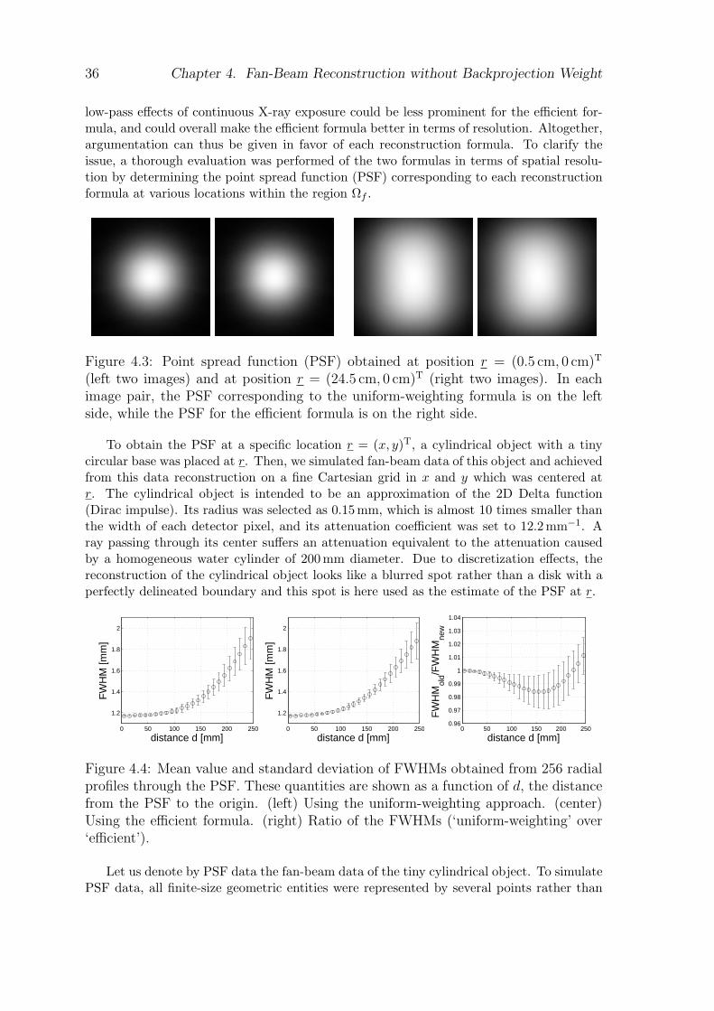
36 Chapter 4. Fan-Beam Reconstruction without Backprojection Weight
low-pass effects of continuous X-ray exposure could be less prominent for the efficient for-mula, and could overall make the efficient formula better in terms of resolution. Altogether,argumentation can thus be given in favor of each reconstruction formula. To clarify theissue, a thorough evaluation was performed of the two formulas in terms of spatial resolu-tion by determining the point spread function (PSF) corresponding to each reconstructionformula at various locations within the region Ωf .
Figure 4.3: Point spread function (PSF) obtained at position r = (0.5 cm, 0 cm)T
(left two images) and at position r = (24.5 cm, 0 cm)T (right two images). In eachimage pair, the PSF corresponding to the uniform-weighting formula is on the leftside, while the PSF for the efficient formula is on the right side.
To obtain the PSF at a specific location r = (x, y)T, a cylindrical object with a tinycircular base was placed at r. Then, we simulated fan-beam data of this object and achievedfrom this data reconstruction on a fine Cartesian grid in x and y which was centered atr. The cylindrical object is intended to be an approximation of the 2D Delta function(Dirac impulse). Its radius was selected as 0.15mm, which is almost 10 times smaller thanthe width of each detector pixel, and its attenuation coefficient was set to 12.2mm−1. Aray passing through its center suffers an attenuation equivalent to the attenuation causedby a homogeneous water cylinder of 200mm diameter. Due to discretization effects, thereconstruction of the cylindrical object looks like a blurred spot rather than a disk with aperfectly delineated boundary and this spot is here used as the estimate of the PSF at r.
0 50 100 150 200 250
1.2
1.4
1.6
1.8
2
distance d [mm]
FW
HM
[mm
]
0 50 100 150 200 250
1.2
1.4
1.6
1.8
2
distance d [mm]
FW
HM
[mm
]
0 50 100 150 200 2500.96
0.97
0.98
0.99
1
1.01
1.02
1.03
1.04
distance d [mm]
FW
HM
old/F
WH
Mne
w
Figure 4.4: Mean value and standard deviation of FWHMs obtained from 256 radialprofiles through the PSF. These quantities are shown as a function of d, the distancefrom the PSF to the origin. (left) Using the uniform-weighting approach. (center)Using the efficient formula. (right) Ratio of the FWHMs (‘uniform-weighting’ over‘efficient’).
Let us denote by PSF data the fan-beam data of the tiny cylindrical object. To simulatePSF data, all finite-size geometric entities were represented by several points rather than
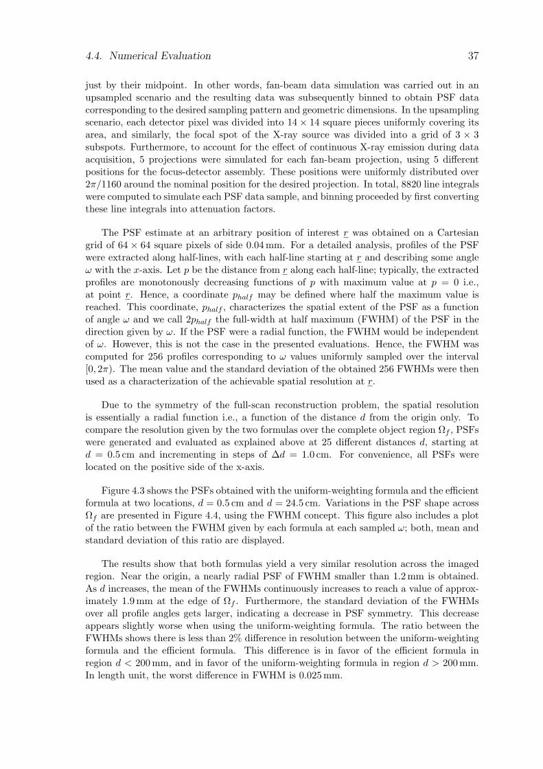
4.4. Numerical Evaluation 37
just by their midpoint. In other words, fan-beam data simulation was carried out in anupsampled scenario and the resulting data was subsequently binned to obtain PSF datacorresponding to the desired sampling pattern and geometric dimensions. In the upsamplingscenario, each detector pixel was divided into 14× 14 square pieces uniformly covering itsarea, and similarly, the focal spot of the X-ray source was divided into a grid of 3 × 3subspots. Furthermore, to account for the effect of continuous X-ray emission during dataacquisition, 5 projections were simulated for each fan-beam projection, using 5 differentpositions for the focus-detector assembly. These positions were uniformly distributed over2π/1160 around the nominal position for the desired projection. In total, 8820 line integralswere computed to simulate each PSF data sample, and binning proceeded by first convertingthese line integrals into attenuation factors.
The PSF estimate at an arbitrary position of interest r was obtained on a Cartesiangrid of 64 × 64 square pixels of side 0.04mm. For a detailed analysis, profiles of the PSFwere extracted along half-lines, with each half-line starting at r and describing some angleω with the x-axis. Let p be the distance from r along each half-line; typically, the extractedprofiles are monotonously decreasing functions of p with maximum value at p = 0 i.e.,at point r. Hence, a coordinate phalf may be defined where half the maximum value isreached. This coordinate, phalf , characterizes the spatial extent of the PSF as a functionof angle ω and we call 2phalf the full-width at half maximum (FWHM) of the PSF in thedirection given by ω. If the PSF were a radial function, the FWHM would be independentof ω. However, this is not the case in the presented evaluations. Hence, the FWHM wascomputed for 256 profiles corresponding to ω values uniformly sampled over the interval[0, 2π). The mean value and the standard deviation of the obtained 256 FWHMs were thenused as a characterization of the achievable spatial resolution at r.
Due to the symmetry of the full-scan reconstruction problem, the spatial resolutionis essentially a radial function i.e., a function of the distance d from the origin only. Tocompare the resolution given by the two formulas over the complete object region Ωf , PSFswere generated and evaluated as explained above at 25 different distances d, starting atd = 0.5 cm and incrementing in steps of ∆d = 1.0 cm. For convenience, all PSFs werelocated on the positive side of the x-axis.
Figure 4.3 shows the PSFs obtained with the uniform-weighting formula and the efficientformula at two locations, d = 0.5 cm and d = 24.5 cm. Variations in the PSF shape acrossΩf are presented in Figure 4.4, using the FWHM concept. This figure also includes a plotof the ratio between the FWHM given by each formula at each sampled ω; both, mean andstandard deviation of this ratio are displayed.
The results show that both formulas yield a very similar resolution across the imagedregion. Near the origin, a nearly radial PSF of FWHM smaller than 1.2mm is obtained.As d increases, the mean of the FWHMs continuously increases to reach a value of approx-imately 1.9mm at the edge of Ωf . Furthermore, the standard deviation of the FWHMsover all profile angles gets larger, indicating a decrease in PSF symmetry. This decreaseappears slightly worse when using the uniform-weighting formula. The ratio between theFWHMs shows there is less than 2% difference in resolution between the uniform-weightingformula and the efficient formula. This difference is in favor of the efficient formula inregion d < 200 mm, and in favor of the uniform-weighting formula in region d > 200mm.In length unit, the worst difference in FWHM is 0.025mm.
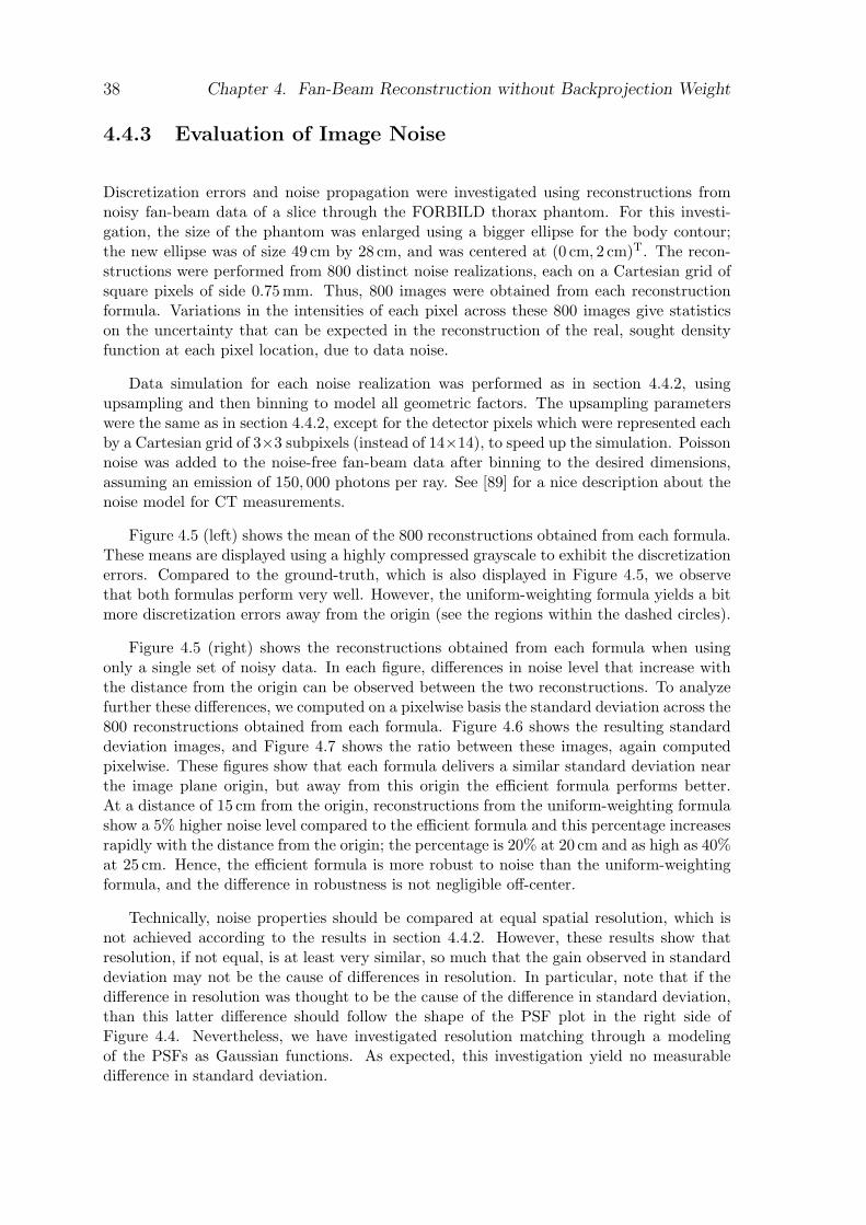
38 Chapter 4. Fan-Beam Reconstruction without Backprojection Weight
4.4.3 Evaluation of Image Noise
Discretization errors and noise propagation were investigated using reconstructions fromnoisy fan-beam data of a slice through the FORBILD thorax phantom. For this investi-gation, the size of the phantom was enlarged using a bigger ellipse for the body contour;the new ellipse was of size 49 cm by 28 cm, and was centered at (0 cm, 2 cm)T. The recon-structions were performed from 800 distinct noise realizations, each on a Cartesian grid ofsquare pixels of side 0.75 mm. Thus, 800 images were obtained from each reconstructionformula. Variations in the intensities of each pixel across these 800 images give statisticson the uncertainty that can be expected in the reconstruction of the real, sought densityfunction at each pixel location, due to data noise.
Data simulation for each noise realization was performed as in section 4.4.2, usingupsampling and then binning to model all geometric factors. The upsampling parameterswere the same as in section 4.4.2, except for the detector pixels which were represented eachby a Cartesian grid of 3×3 subpixels (instead of 14×14), to speed up the simulation. Poissonnoise was added to the noise-free fan-beam data after binning to the desired dimensions,assuming an emission of 150, 000 photons per ray. See [89] for a nice description about thenoise model for CT measurements.
Figure 4.5 (left) shows the mean of the 800 reconstructions obtained from each formula.These means are displayed using a highly compressed grayscale to exhibit the discretizationerrors. Compared to the ground-truth, which is also displayed in Figure 4.5, we observethat both formulas perform very well. However, the uniform-weighting formula yields a bitmore discretization errors away from the origin (see the regions within the dashed circles).
Figure 4.5 (right) shows the reconstructions obtained from each formula when usingonly a single set of noisy data. In each figure, differences in noise level that increase withthe distance from the origin can be observed between the two reconstructions. To analyzefurther these differences, we computed on a pixelwise basis the standard deviation across the800 reconstructions obtained from each formula. Figure 4.6 shows the resulting standarddeviation images, and Figure 4.7 shows the ratio between these images, again computedpixelwise. These figures show that each formula delivers a similar standard deviation nearthe image plane origin, but away from this origin the efficient formula performs better.At a distance of 15 cm from the origin, reconstructions from the uniform-weighting formulashow a 5% higher noise level compared to the efficient formula and this percentage increasesrapidly with the distance from the origin; the percentage is 20% at 20 cm and as high as 40%at 25 cm. Hence, the efficient formula is more robust to noise than the uniform-weightingformula, and the difference in robustness is not negligible off-center.
Technically, noise properties should be compared at equal spatial resolution, which isnot achieved according to the results in section 4.4.2. However, these results show thatresolution, if not equal, is at least very similar, so much that the gain observed in standarddeviation may not be the cause of differences in resolution. In particular, note that if thedifference in resolution was thought to be the cause of the difference in standard deviation,than this latter difference should follow the shape of the PSF plot in the right side ofFigure 4.4. Nevertheless, we have investigated resolution matching through a modelingof the PSFs as Gaussian functions. As expected, this investigation yield no measurabledifference in standard deviation.
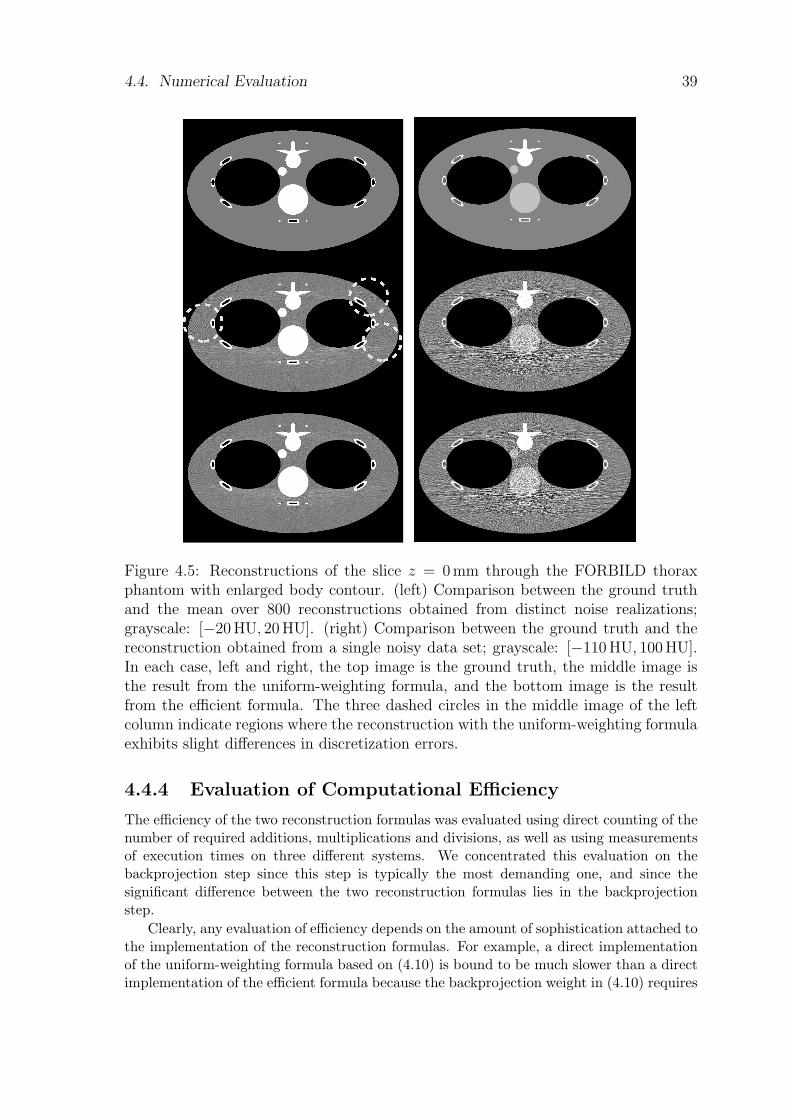
4.4. Numerical Evaluation 39
Figure 4.5: Reconstructions of the slice z = 0mm through the FORBILD thoraxphantom with enlarged body contour. (left) Comparison between the ground truthand the mean over 800 reconstructions obtained from distinct noise realizations;grayscale: [−20 HU, 20 HU]. (right) Comparison between the ground truth and thereconstruction obtained from a single noisy data set; grayscale: [−110 HU, 100 HU].In each case, left and right, the top image is the ground truth, the middle image isthe result from the uniform-weighting formula, and the bottom image is the resultfrom the efficient formula. The three dashed circles in the middle image of the leftcolumn indicate regions where the reconstruction with the uniform-weighting formulaexhibits slight differences in discretization errors.
4.4.4 Evaluation of Computational Efficiency
The efficiency of the two reconstruction formulas was evaluated using direct counting of thenumber of required additions, multiplications and divisions, as well as using measurementsof execution times on three different systems. We concentrated this evaluation on thebackprojection step since this step is typically the most demanding one, and since thesignificant difference between the two reconstruction formulas lies in the backprojectionstep.
Clearly, any evaluation of efficiency depends on the amount of sophistication attached tothe implementation of the reconstruction formulas. For example, a direct implementationof the uniform-weighting formula based on (4.10) is bound to be much slower than a directimplementation of the efficient formula because the backprojection weight in (4.10) requires
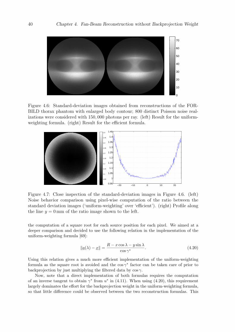
40 Chapter 4. Fan-Beam Reconstruction without Backprojection Weight
0
10
20
30
40
50
60
70
Figure 4.6: Standard-deviation images obtained from reconstructions of the FOR-BILD thorax phantom with enlarged body contour; 800 distinct Poisson noise real-izations were considered with 150, 000 photons per ray. (left) Result for the uniform-weighting formula. (right) Result for the efficient formula.
1
1.05
1.1
1.15
1.2
1.25
1.3
1.35
1.4
1.45
1.5
−20 −10 0 10 200.95
1
1.05
1.1
1.15
1.2
1.25
1.3
1.35
1.4
1.45
Figure 4.7: Close inspection of the standard-deviation images in Figure 4.6. (left)Noise behavior comparison using pixel-wise computation of the ratio between thestandard deviation images (‘uniform-weighting’ over ‘efficient’). (right) Profile alongthe line y = 0 mm of the ratio image shown to the left.
the computation of a square root for each source position for each pixel. We aimed at adeeper comparison and decided to use the following relation in the implementation of theuniform-weighting formula [69]:
‖a(λ)− x‖ =R− x cosλ− y sinλ
cos γ∗. (4.20)
Using this relation gives a much more efficient implementation of the uniform-weightingformula as the square root is avoided and the cos γ∗ factor can be taken care of prior tobackprojection by just multiplying the filtered data by cos γ.
Now, note that a direct implementation of both formulas requires the computationof an inverse tangent to obtain γ∗ from u∗ in (4.11). When using (4.20), this requirementlargely dominates the effort for the backprojection weight in the uniform-weighting formula,so that little difference could be observed between the two reconstruction formulas. This
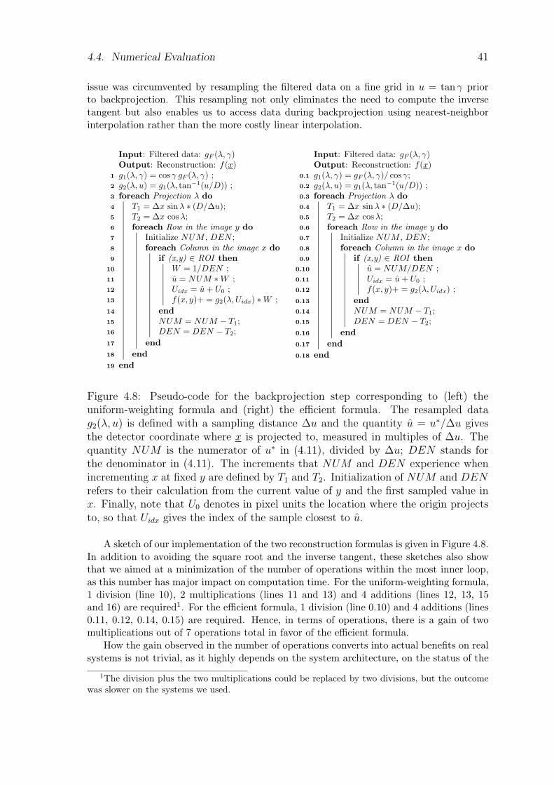
4.4. Numerical Evaluation 41
issue was circumvented by resampling the filtered data on a fine grid in u = tan γ priorto backprojection. This resampling not only eliminates the need to compute the inversetangent but also enables us to access data during backprojection using nearest-neighborinterpolation rather than the more costly linear interpolation.
Input: Filtered data: gF (λ, γ)Output: Reconstruction: f(x)g1(λ, γ) = cos γ gF (λ, γ) ;1
g2(λ, u) = g1(λ, tan−1(u/D)) ;2
foreach Projection λ do3
T1 = ∆x sin λ ∗ (D/∆u);4
T2 = ∆x cosλ;5
foreach Row in the image y do6
Initialize NUM , DEN ;7
foreach Column in the image x do8
if (x,y) ∈ ROI then9
W = 1/DEN ;10
u = NUM ∗ W ;11
Uidx = u + U0 ;12
f(x, y)+ = g2(λ, Uidx) ∗ W ;13
end14
NUM = NUM − T1;15
DEN = DEN − T2;16
end17
end18
end19
Input: Filtered data: gF (λ, γ)Output: Reconstruction: f(x)g1(λ, γ) = gF (λ, γ)/ cos γ;0.1
g2(λ, u) = g1(λ, tan−1(u/D)) ;0.2
foreach Projection λ do0.3
T1 = ∆x sin λ ∗ (D/∆u);0.4
T2 = ∆x cosλ;0.5
foreach Row in the image y do0.6
Initialize NUM , DEN ;0.7
foreach Column in the image x do0.8
if (x,y) ∈ ROI then0.9
u = NUM/DEN ;0.10
Uidx = u + U0 ;0.11
f(x, y)+ = g2(λ, Uidx) ;0.12
end0.13
NUM = NUM − T1;0.14
DEN = DEN − T2;0.15
end0.16
end0.17
end0.18
Figure 4.8: Pseudo-code for the backprojection step corresponding to (left) theuniform-weighting formula and (right) the efficient formula. The resampled datag2(λ, u) is defined with a sampling distance ∆u and the quantity u = u∗/∆u givesthe detector coordinate where x is projected to, measured in multiples of ∆u. Thequantity NUM is the numerator of u∗ in (4.11), divided by ∆u; DEN stands forthe denominator in (4.11). The increments that NUM and DEN experience whenincrementing x at fixed y are defined by T1 and T2. Initialization of NUM and DENrefers to their calculation from the current value of y and the first sampled value inx. Finally, note that U0 denotes in pixel units the location where the origin projectsto, so that Uidx gives the index of the sample closest to u.
A sketch of our implementation of the two reconstruction formulas is given in Figure 4.8.In addition to avoiding the square root and the inverse tangent, these sketches also showthat we aimed at a minimization of the number of operations within the most inner loop,as this number has major impact on computation time. For the uniform-weighting formula,1 division (line 10), 2 multiplications (lines 11 and 13) and 4 additions (lines 12, 13, 15and 16) are required1. For the efficient formula, 1 division (line 0.10) and 4 additions (lines0.11, 0.12, 0.14, 0.15) are required. Hence, in terms of operations, there is a gain of twomultiplications out of 7 operations total in favor of the efficient formula.
How the gain observed in the number of operations converts into actual benefits on realsystems is not trivial, as it highly depends on the system architecture, on the status of the
1The division plus the two multiplications could be replaced by two divisions, but the outcomewas slower on the systems we used.
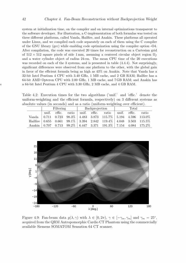
42 Chapter 4. Fan-Beam Reconstruction without Backprojection Weight
system at initialization time, on the compiler and on internal optimizations transparent tothe software developer. For illustration, a C-implementation of both formulas was tested onthree different platforms, called Vanda, Hailfire, and Anakin. These platforms all operatedunder Linux, and we compiled each code separately on each of them using the C compilerof the GNU library (gcc) while enabling code optimization using the compiler option -O4.After compilation, the code was executed 20 times for reconstruction on a Cartesian gridof 512 × 512 square pixels of side 1 mm, assuming a centered circular object region Ωf
and a water cylinder object of radius 24 cm. The mean CPU time of the 20 executionswas recorded on each of the 3 systems, and is presented in table (4.4.4). Not surprisingly,significant differences were observed from one platform to the other, with the global gainin favor of the efficient formula being as high as 43% on Anakin. Note that Vanda has a32-bit Intel Pentium 4 CPU with 3.40 GHz, 1 MB cache, and 2 GB RAM; Hailfire has a64-bit AMD Opteron CPU with 2.00 GHz, 1 MB cache, and 7GB RAM; and Anakin hasa 64-bit Intel Pentium 4 CPU with 3.30 GHz, 2 MB cache, and 4 GB RAM.results
Table 4.2: Execution times for the two algorithms (’unif.’ and ’effic.’ denote theuniform-weighting and the efficient formula, respectively) on 3 different systems asabsolute values (in seconds) and as a ratio (uniform-weighting over efficient).
Filtering Backprojection Totalunif. effic. ratio unif. effic. ratio unif. effic. ratio
Vanda 0.711 0.723 98.3% 4.483 3.873 115.7% 5.194 4.596 113.0%Hailfire 0.655 0.661 99.1% 3.394 2.842 119.4% 4.048 3.503 115.5%Anakin 0.707 0.713 99.2% 6.447 3.371 191.3% 7.154 4.084 175.2%
λ [deg.]
γ [d
eg.]
−180 −120 −60 0 60 120 180−24
−19
−14
−9
−4
1
6
11
16
21
Figure 4.9: Fan-beam data g(λ, γ) with λ ∈ [0, 2π), γ ∈ [−γm, γm] and γm = 25,acquired from the QRM Antropomorphic Cardio CT Phantom using the commerciallyavailable Siemens SOMATOM Sensation 64 CT scanner.
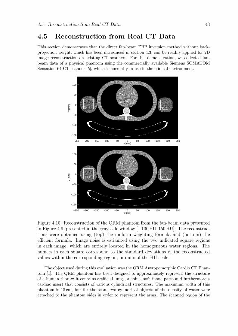
4.5. Reconstruction from Real CT Data 43
4.5 Reconstruction from Real CT Data
This section demonstrates that the direct fan-beam FBP inversion method without back-projection weight, which has been introduced in section 4.3, can be readily applied for 2Dimage reconstruction on existing CT scanners. For this demonstration, we collected fan-beam data of a physical phantom using the commercially available Siemens SOMATOMSensation 64 CT scanner [5], which is currently in use in the clinical environment.
x [mm]
y [m
m]
34.5 31.1
−250 −200 −150 −100 −50 0 50 100 150 200 250
−150
−100
−50
0
50
100
x [mm]
y [m
m]
30.1 27.5
−250 −200 −150 −100 −50 0 50 100 150 200 250
−150
−100
−50
0
50
100
Figure 4.10: Reconstruction of the QRM phantom from the fan-beam data presentedin Figure 4.9, presented in the grayscale window [−100 HU, 150 HU]. The reconstruc-tions were obtained using (top) the uniform weighting formula and (bottom) theefficient formula. Image noise is estiamted using the two indicated square regionsin each image, which are entirely located in the homogeneous water regions. Thenumers in each square correspond to the standard deviations of the reconstructedvalues within the corresponding region, in units of the HU scale.
The object used during this evaluation was the QRM Antropomorphic Cardio CT Phan-tom [1]. The QRM phantom has been designed to approximately represent the structureof a human thorax; it contains artificial lungs, a spine, soft tissue parts and furthermore acardiac insert that consists of various cylindrical structures. The maximum width of thisphantom is 15 cm, but for the scan, two cylindrical objects of the density of water wereattached to the phantom sides in order to represent the arms. The scanned region of the
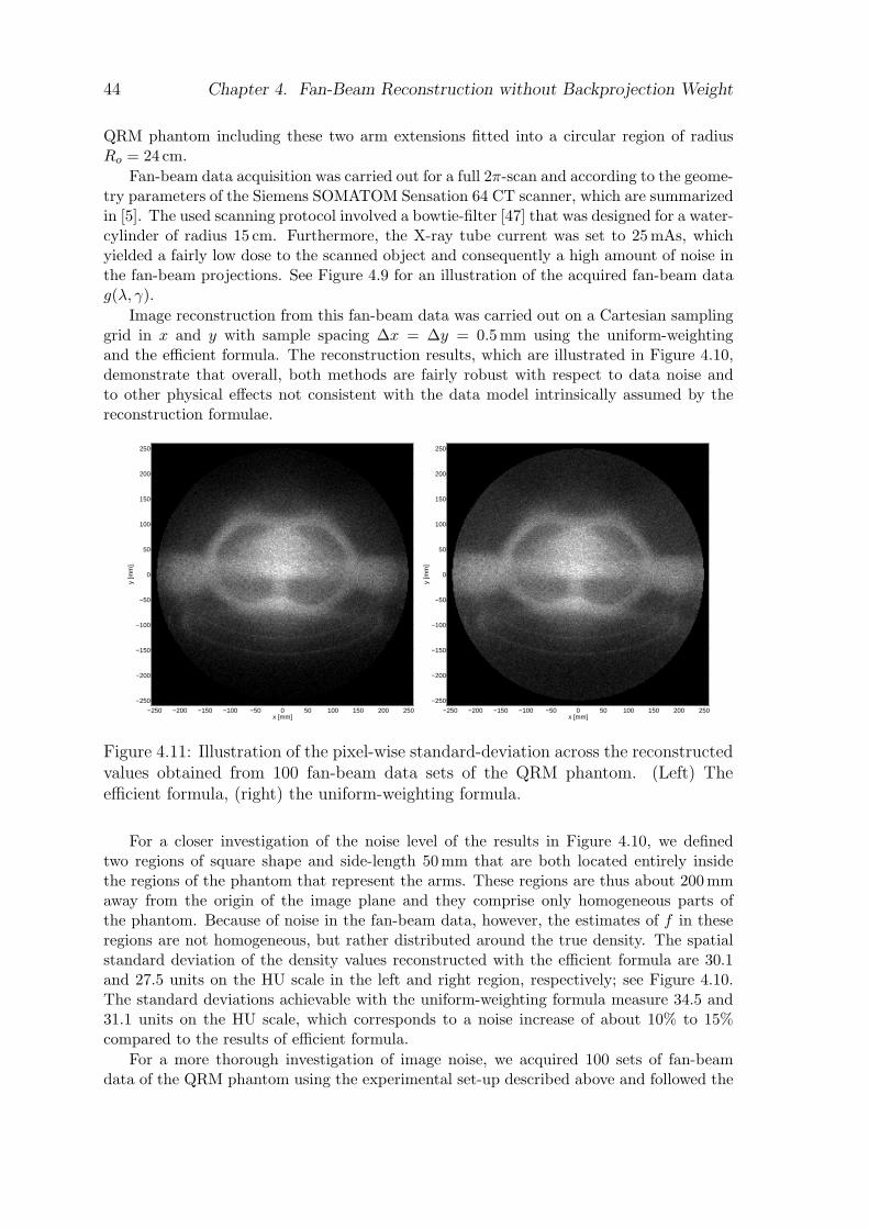
44 Chapter 4. Fan-Beam Reconstruction without Backprojection Weight
QRM phantom including these two arm extensions fitted into a circular region of radiusRo = 24 cm.
Fan-beam data acquisition was carried out for a full 2π-scan and according to the geome-try parameters of the Siemens SOMATOM Sensation 64 CT scanner, which are summarizedin [5]. The used scanning protocol involved a bowtie-filter [47] that was designed for a water-cylinder of radius 15 cm. Furthermore, the X-ray tube current was set to 25 mAs, whichyielded a fairly low dose to the scanned object and consequently a high amount of noise inthe fan-beam projections. See Figure 4.9 for an illustration of the acquired fan-beam datag(λ, γ).
Image reconstruction from this fan-beam data was carried out on a Cartesian samplinggrid in x and y with sample spacing ∆x = ∆y = 0.5mm using the uniform-weightingand the efficient formula. The reconstruction results, which are illustrated in Figure 4.10,demonstrate that overall, both methods are fairly robust with respect to data noise andto other physical effects not consistent with the data model intrinsically assumed by thereconstruction formulae.
x [mm]
y [m
m]
−250 −200 −150 −100 −50 0 50 100 150 200 250
−250
−200
−150
−100
−50
0
50
100
150
200
250
x [mm]
y [m
m]
−250 −200 −150 −100 −50 0 50 100 150 200 250
−250
−200
−150
−100
−50
0
50
100
150
200
250
Figure 4.11: Illustration of the pixel-wise standard-deviation across the reconstructedvalues obtained from 100 fan-beam data sets of the QRM phantom. (Left) Theefficient formula, (right) the uniform-weighting formula.
For a closer investigation of the noise level of the results in Figure 4.10, we definedtwo regions of square shape and side-length 50mm that are both located entirely insidethe regions of the phantom that represent the arms. These regions are thus about 200mmaway from the origin of the image plane and they comprise only homogeneous parts ofthe phantom. Because of noise in the fan-beam data, however, the estimates of f in theseregions are not homogeneous, but rather distributed around the true density. The spatialstandard deviation of the density values reconstructed with the efficient formula are 30.1and 27.5 units on the HU scale in the left and right region, respectively; see Figure 4.10.The standard deviations achievable with the uniform-weighting formula measure 34.5 and31.1 units on the HU scale, which corresponds to a noise increase of about 10% to 15%compared to the results of efficient formula.
For a more thorough investigation of image noise, we acquired 100 sets of fan-beamdata of the QRM phantom using the experimental set-up described above and followed the
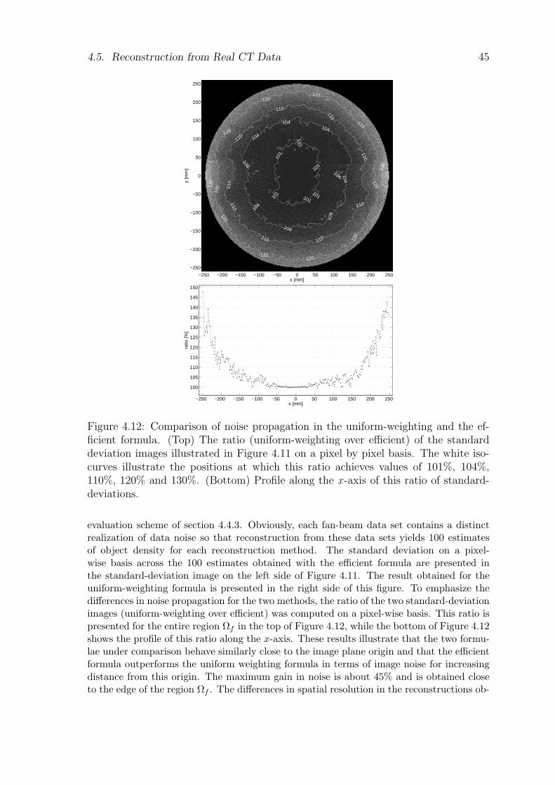
4.5. Reconstruction from Real CT Data 45
101
101
101
101
101
101
104
104
104
104
104
104104
104
104
110
110 110
110
110
110
110
110
110
120
120120
120
120
120
120120
120
12013
0
130
x [mm]
y [m
m]
−250 −200 −150 −100 −50 0 50 100 150 200 250
−250
−200
−150
−100
−50
0
50
100
150
200
250
−250 −200 −150 −100 −50 0 50 100 150 200 250
100
105
110
115
120
125
130
135
140
145
150
x [mm]
ratio
[%]
Figure 4.12: Comparison of noise propagation in the uniform-weighting and the ef-ficient formula. (Top) The ratio (uniform-weighting over efficient) of the standarddeviation images illustrated in Figure 4.11 on a pixel by pixel basis. The white iso-curves illustrate the positions at which this ratio achieves values of 101%, 104%,110%, 120% and 130%. (Bottom) Profile along the x-axis of this ratio of standard-deviations.
evaluation scheme of section 4.4.3. Obviously, each fan-beam data set contains a distinctrealization of data noise so that reconstruction from these data sets yields 100 estimatesof object density for each reconstruction method. The standard deviation on a pixel-wise basis across the 100 estimates obtained with the efficient formula are presented inthe standard-deviation image on the left side of Figure 4.11. The result obtained for theuniform-weighting formula is presented in the right side of this figure. To emphasize thedifferences in noise propagation for the two methods, the ratio of the two standard-deviationimages (uniform-weighting over efficient) was computed on a pixel-wise basis. This ratio ispresented for the entire region Ωf in the top of Figure 4.12, while the bottom of Figure 4.12shows the profile of this ratio along the x-axis. These results illustrate that the two formu-lae under comparison behave similarly close to the image plane origin and that the efficientformula outperforms the uniform weighting formula in terms of image noise for increasingdistance from this origin. The maximum gain in noise is about 45% and is obtained closeto the edge of the region Ωf . The differences in spatial resolution in the reconstructions ob-
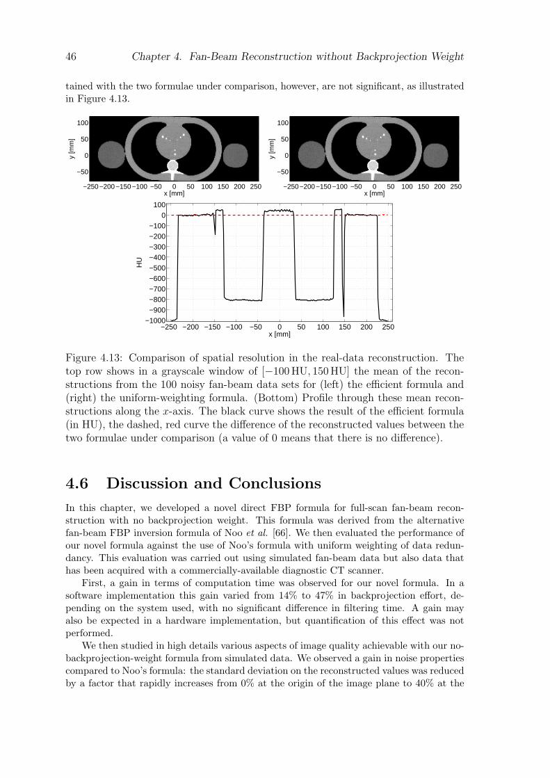
46 Chapter 4. Fan-Beam Reconstruction without Backprojection Weight
tained with the two formulae under comparison, however, are not significant, as illustratedin Figure 4.13.
x [mm]
y [m
m]
−250−200−150−100 −50 0 50 100 150 200 250
−50
0
50
100
x [mm]
y [m
m]
−250−200−150−100 −50 0 50 100 150 200 250
−50
0
50
100
−250 −200 −150 −100 −50 0 50 100 150 200 250−1000−900
−800−700−600
−500−400
−300−200−100
0100
x [mm]
HU
Figure 4.13: Comparison of spatial resolution in the real-data reconstruction. Thetop row shows in a grayscale window of [−100 HU, 150 HU] the mean of the recon-structions from the 100 noisy fan-beam data sets for (left) the efficient formula and(right) the uniform-weighting formula. (Bottom) Profile through these mean recon-structions along the x-axis. The black curve shows the result of the efficient formula(in HU), the dashed, red curve the difference of the reconstructed values between thetwo formulae under comparison (a value of 0 means that there is no difference).
4.6 Discussion and Conclusions
In this chapter, we developed a novel direct FBP formula for full-scan fan-beam recon-struction with no backprojection weight. This formula was derived from the alternativefan-beam FBP inversion formula of Noo et al. [66]. We then evaluated the performance ofour novel formula against the use of Noo’s formula with uniform weighting of data redun-dancy. This evaluation was carried out using simulated fan-beam data but also data thathas been acquired with a commercially-available diagnostic CT scanner.
First, a gain in terms of computation time was observed for our novel formula. In asoftware implementation this gain varied from 14% to 47% in backprojection effort, de-pending on the system used, with no significant difference in filtering time. A gain mayalso be expected in a hardware implementation, but quantification of this effect was notperformed.
We then studied in high details various aspects of image quality achievable with our no-backprojection-weight formula from simulated data. We observed a gain in noise propertiescompared to Noo’s formula: the standard deviation on the reconstructed values was reducedby a factor that rapidly increases from 0% at the origin of the image plane to 40% at the
4.6. Discussion and Conclusions 47
edge of the region Ωf ; this improvement may be significant for large patients. On the otherhand, spatial resolution and discretization errors appeared for both formulae very similaracross the object support region Ωf .
We also investigated image reconstruction from data collected with a clinical CT scannerand demonstrated that our novel formula is robust with respect to physical effects notcontained in the underlying ray-integral data model. Moreover, improvements in imagenoise were observed compared to the uniform-weighting formula that are quantitativelyalmost identical to those determined previously, in the simulation studies. This advantagemakes our formula an attractive candidate for reconstruction in 2D imaging applicationson diagnostic CT scanners.
Note finally that the novel formula has not been compared against the classical fan-beamFBP method [46], which was described in section 3.2.3. However, a superior performancemay be anticipated, both in computation time and in image quality. The gain in computa-tion time is straightforward since our formula does not require any backprojection weight,while the effort in data filtering is essentially the same. For the gain in image quality,we refer the reader to [94], which shows that the classical formula is less robust to datanoise and discretization errors than the uniform-weighting formula, which we compared thenovel formula to. To achieve this superiority in image quality, it may however be neededto compute g(λ, γ) in equation (4.12) using the approach suggested in [94] rather than ourdiscretization scheme.

48 Chapter 4. Fan-Beam Reconstruction without Backprojection Weight
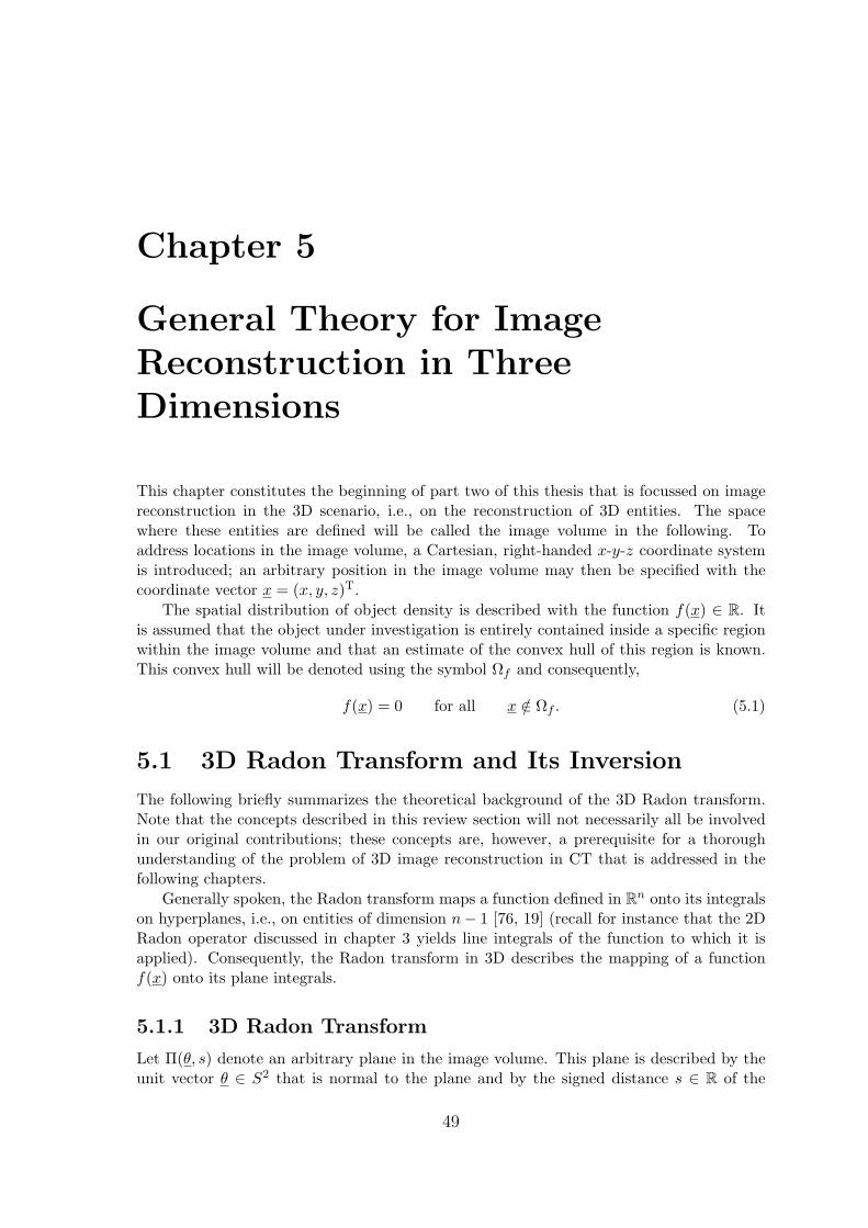
Chapter 5
General Theory for ImageReconstruction in ThreeDimensions
This chapter constitutes the beginning of part two of this thesis that is focussed on imagereconstruction in the 3D scenario, i.e., on the reconstruction of 3D entities. The spacewhere these entities are defined will be called the image volume in the following. Toaddress locations in the image volume, a Cartesian, right-handed x-y-z coordinate systemis introduced; an arbitrary position in the image volume may then be specified with thecoordinate vector x = (x, y, z)T.
The spatial distribution of object density is described with the function f(x) ∈ R. Itis assumed that the object under investigation is entirely contained inside a specific regionwithin the image volume and that an estimate of the convex hull of this region is known.This convex hull will be denoted using the symbol Ωf and consequently,
f(x) = 0 for all x /∈ Ωf . (5.1)
5.1 3D Radon Transform and Its Inversion
The following briefly summarizes the theoretical background of the 3D Radon transform.Note that the concepts described in this review section will not necessarily all be involvedin our original contributions; these concepts are, however, a prerequisite for a thoroughunderstanding of the problem of 3D image reconstruction in CT that is addressed in thefollowing chapters.
Generally spoken, the Radon transform maps a function defined in Rn onto its integralson hyperplanes, i.e., on entities of dimension n− 1 [76, 19] (recall for instance that the 2DRadon operator discussed in chapter 3 yields line integrals of the function to which it isapplied). Consequently, the Radon transform in 3D describes the mapping of a functionf(x) onto its plane integrals.
5.1.1 3D Radon Transform
Let Π(θ, s) denote an arbitrary plane in the image volume. This plane is described by theunit vector θ ∈ S2 that is normal to the plane and by the signed distance s ∈ R of the
49
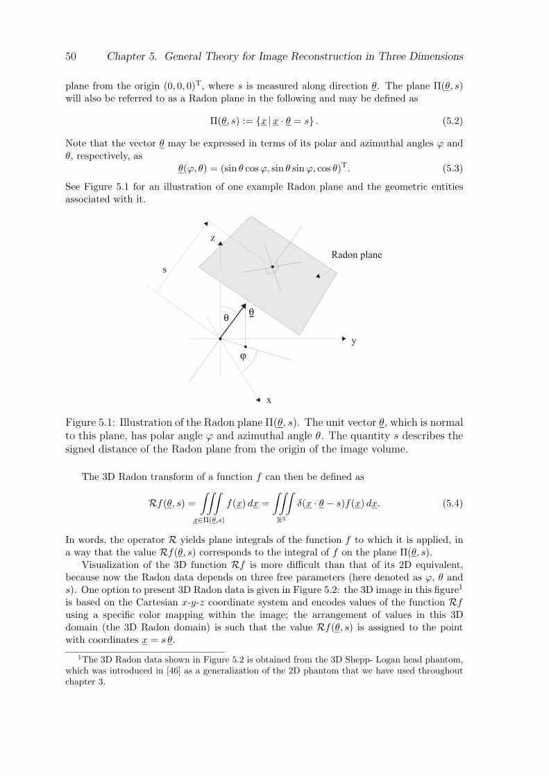
50 Chapter 5. General Theory for Image Reconstruction in Three Dimensions
plane from the origin (0, 0, 0)T, where s is measured along direction θ. The plane Π(θ, s)will also be referred to as a Radon plane in the following and may be defined as
Π(θ, s) := x |x · θ = s . (5.2)
Note that the vector θ may be expressed in terms of its polar and azimuthal angles ϕ andθ, respectively, as
θ(ϕ, θ) = (sin θ cosϕ, sin θ sinϕ, cos θ)T. (5.3)
See Figure 5.1 for an illustration of one example Radon plane and the geometric entitiesassociated with it.
Radon plane
z
x
y
s
Figure 5.1: Illustration of the Radon plane Π(θ, s). The unit vector θ, which is normalto this plane, has polar angle ϕ and azimuthal angle θ. The quantity s describes thesigned distance of the Radon plane from the origin of the image volume.
The 3D Radon transform of a function f can then be defined as
Rf(θ, s) =∫∫∫
x∈Π(θ,s)
f(x) dx =∫∫∫
R3
δ(x · θ − s)f(x) dx. (5.4)
In words, the operator R yields plane integrals of the function f to which it is applied, ina way that the value Rf(θ, s) corresponds to the integral of f on the plane Π(θ, s).
Visualization of the 3D function Rf is more difficult than that of its 2D equivalent,because now the Radon data depends on three free parameters (here denoted as ϕ, θ ands). One option to present 3D Radon data is given in Figure 5.2: the 3D image in this figure1
is based on the Cartesian x-y-z coordinate system and encodes values of the function Rfusing a specific color mapping within the image; the arrangement of values in this 3Ddomain (the 3D Radon domain) is such that the value Rf(θ, s) is assigned to the pointwith coordinates x = s θ.
1The 3D Radon data shown in Figure 5.2 is obtained from the 3D Shepp- Logan head phantom,which was introduced in [46] as a generalization of the 2D phantom that we have used throughoutchapter 3.
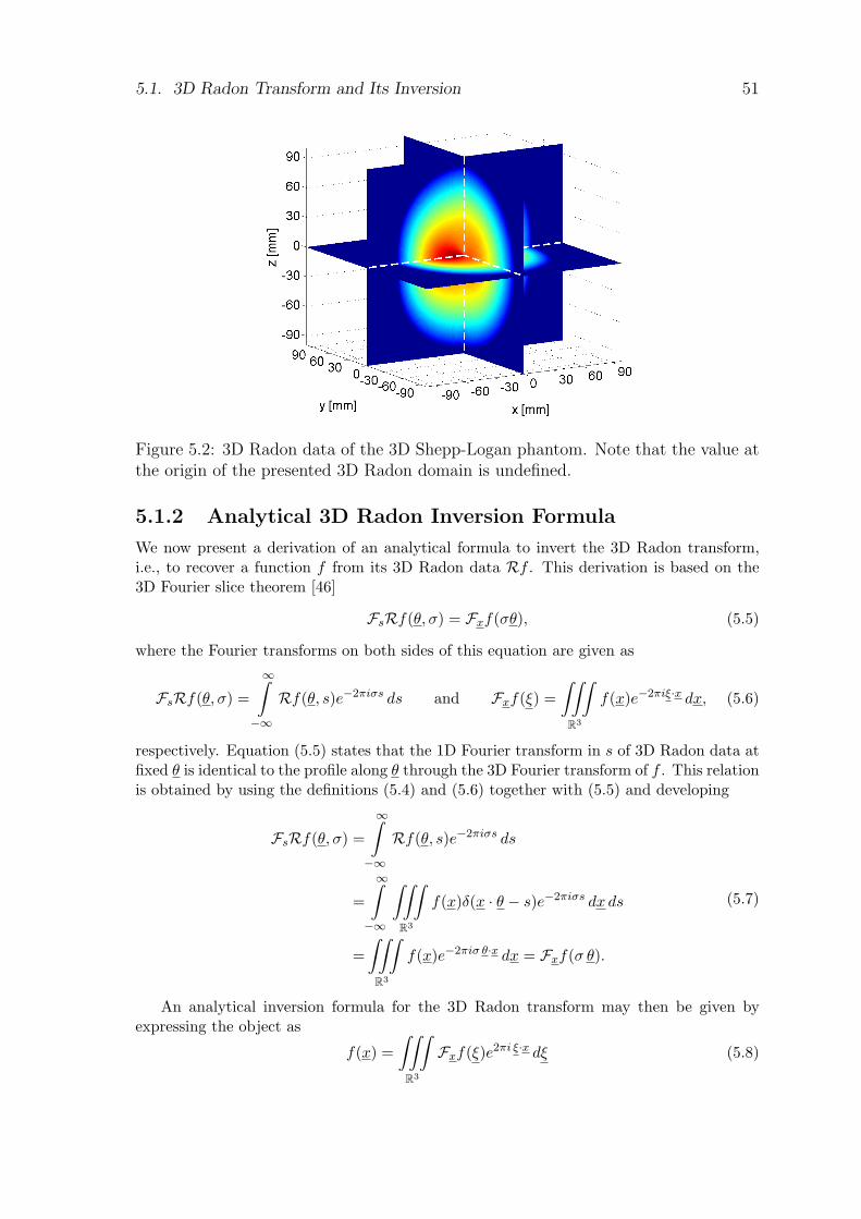
5.1. 3D Radon Transform and Its Inversion 51
Figure 5.2: 3D Radon data of the 3D Shepp-Logan phantom. Note that the value atthe origin of the presented 3D Radon domain is undefined.
5.1.2 Analytical 3D Radon Inversion Formula
We now present a derivation of an analytical formula to invert the 3D Radon transform,i.e., to recover a function f from its 3D Radon data Rf . This derivation is based on the3D Fourier slice theorem [46]
FsRf(θ, σ) = Fxf(σθ), (5.5)
where the Fourier transforms on both sides of this equation are given as
FsRf(θ, σ) =
∞∫
−∞Rf(θ, s)e−2πiσs ds and Fxf(ξ) =
∫∫∫
R3
f(x)e−2πiξ·x dx, (5.6)
respectively. Equation (5.5) states that the 1D Fourier transform in s of 3D Radon data atfixed θ is identical to the profile along θ through the 3D Fourier transform of f . This relationis obtained by using the definitions (5.4) and (5.6) together with (5.5) and developing
FsRf(θ, σ) =
∞∫
−∞Rf(θ, s)e−2πiσs ds
=
∞∫
−∞
∫∫∫
R3
f(x)δ(x · θ − s)e−2πiσs dx ds
=∫∫∫
R3
f(x)e−2πiσ θ·x dx = Fxf(σ θ).
(5.7)
An analytical inversion formula for the 3D Radon transform may then be given byexpressing the object as
f(x) =∫∫∫
R3
Fxf(ξ)e2πi ξ·x dξ (5.8)
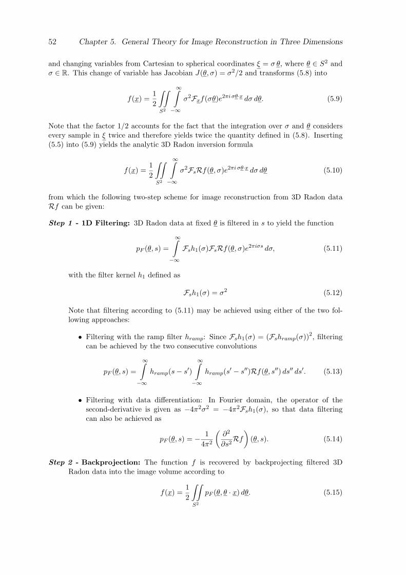
52 Chapter 5. General Theory for Image Reconstruction in Three Dimensions
and changing variables from Cartesian to spherical coordinates ξ = σ θ, where θ ∈ S2 andσ ∈ R. This change of variable has Jacobian J(θ, σ) = σ2/2 and transforms (5.8) into
f(x) =12
∫∫
S2
∞∫
−∞σ2Fxf(σθ)e2πi σθ·x dσ dθ. (5.9)
Note that the factor 1/2 accounts for the fact that the integration over σ and θ considersevery sample in ξ twice and therefore yields twice the quantity defined in (5.8). Inserting(5.5) into (5.9) yields the analytic 3D Radon inversion formula
f(x) =12
∫∫
S2
∞∫
−∞σ2FsRf(θ, σ)e2πi σθ·x dσ dθ (5.10)
from which the following two-step scheme for image reconstruction from 3D Radon dataRf can be given:
Step 1 - 1D Filtering: 3D Radon data at fixed θ is filtered in s to yield the function
pF (θ, s) =
∞∫
−∞Fsh1(σ)FsRf(θ, σ)e2πiσs dσ, (5.11)
with the filter kernel h1 defined as
Fsh1(σ) = σ2 (5.12)
Note that filtering according to (5.11) may be achieved using either of the two fol-lowing approaches:
• Filtering with the ramp filter hramp: Since Fsh1(σ) = (Fshramp(σ))2, filteringcan be achieved by the two consecutive convolutions
pF (θ, s) =
∞∫
−∞hramp(s− s′)
∞∫
−∞hramp(s′ − s′′)Rf(θ, s′′) ds′′ ds′. (5.13)
• Filtering with data differentiation: In Fourier domain, the operator of thesecond-derivative is given as −4π2σ2 = −4π2Fsh1(σ), so that data filteringcan also be achieved as
pF (θ, s) = − 14π2
(∂2
∂s2Rf
)(θ, s). (5.14)
Step 2 - Backprojection: The function f is recovered by backprojecting filtered 3DRadon data into the image volume according to
f(x) =12
∫∫
S2
pF (θ, θ · x) dθ. (5.15)
5.2. Image Reconstruction in the Cone-Beam Geometry 53
Note that the convolution described in (5.13) corresponds to a global filtering operationand requiresRf to be known over the entire support of s. Filtering using data differentiationaccording to (5.14), in contrast, is a local operation which requires only knowledge of valuesofRf in a neighborhood of the sample s at which pF is desired. The latter filtering approachis thus preferable for practical implementation, and substituting (5.14) into (5.15) yieldsthe well-known classical analytical 3D Radon inversion formula [46]:
f(x) = − 18π2
∫∫
S2
(∂2
∂s2Rf
)(θ, s)
∣∣∣∣s=x·θ
dθ. (5.16)
Equation (5.16) describes a stable analytical way of recovering the function f from its3D Radon data; a practical and efficient algorithmic implementation of this formula hasbeen suggested by [58]. Note that the reconstruction at x requires filtered 3D Radon datafor all θ ∈ S2, using for each θ the sample of pF at (θ, x · θ). Geometrically that means thatimage reconstruction at an arbitrary point x according to (5.16) requires the values of Rffor all Radon planes through a neighborhood of x. In other words, reconstruction of f(x)based on equation (5.16) thus yields a valid result if the function (∂2/∂s2)Rf is known overthe entire surface of the smallest sphere in 3D Radon domain that contains the origin andthe point x.
5.2 Image Reconstruction in the Cone-Beam Ge-
ometry
In the following, we address the problem of 3D image reconstruction from 2D projectionsacquired in the geometry of state-of-the-art medical C-arm systems or multi-row diagnosticCT scanners.
5.2.1 General Cone-beam Acquisition Geometry
According to the model described in chapter 2, each 2D projection image acquired on X-rayCT systems provides access to integral values of the object density function along the raysthat connect the elements of the 2D detector to the corresponding X-ray source point; eachof these sets of rays thus forms geometrically a cone-beam (CB) in the image volume.
Here and in the following, we assume that projection data is acquired with the X-ray source point moving along a connected curve a(λ) in space, which we will call thesource trajectory. The quantity λ corresponds to the curve parameter and is restricted toλ ∈ [λmin, λmax]. We assume that the source trajectory does not intersect with the convexregion Ωf that encloses the object.
X-ray measurements then yield samples of the function
g(λ, α) =
∞∫
0
f(a(λ) + tα) dt, (5.17)
where α ∈ S2 is used to describe the unit direction of the measurement ray. Note that (5.17)corresponds to a general definition of CB data; in practice, the set of potential realizationsof the vector α depends on the geometry of the detector that is used for data acquisition,as will be discussed in chapter 6. Values of g will be called CB data from now on, and CB
54 Chapter 5. General Theory for Image Reconstruction in Three Dimensions
data at fixed λ will be referred to as a CB projection. If all non-zero values of the functiong at fixed λ are known, the corresponding CB projection is called non-truncated.
5.2.2 Cone-Beam Reconstruction in General
This section briefly summarizes the fundamentals about 3D CB reconstruction theory. Ourgoal is not to provide a detailed topical review, but to describe the major theoreticaldevelopments as they occurred over the last about 30 years; for further information see[82, 62, 18, 21, 12] or others.
One of the major difficulties of the 3D CB reconstruction problem lies in the fact thatCB data samples are not related to samples of the 3D Radon transform in a direct andstraight-forward manner. In this respect, the reconstruction problem fundamentally differsfrom that in 2D fan-beam tomography: in the fan-beam scenario, data acquisition directlydelivers 2D Radon values so that reconstruction can be easily accomplished by using 2DRadon inversion formulae with some minor modifications, as shown in chapter 3. In 3D,however, a direct generalization like that is not possible.
Some of the first methods suggested to achieve CB image reconstruction were basedon approximate inversion formulae. Feldkamp et al., for instance, suggested a practicalreconstruction approach for CB data acquired along a full circular source trajectory [33].Feldkamp’s approach was derived as a heuristic generalization of the classical 2D fan-beamreconstruction method; it possesses an efficient FBP scheme and has therefore been con-sidered in various clinical applications. Over the years, many variations of the Feldkampalgorithm have been suggested, some of which are described in [82], but these reconstructionapproaches yield in general inexact results, and because they lack a thorough theoreticalfoundation, the degree of artifacts arising in the reconstruction results is in general not easyto predict.
The early 1980s brought some significant breakthroughs in the analytical CB recon-struction theory, as summarized, for instance, in the review papers [17, 81]. Advance-ments were mainly driven by the contributions of Tuy [83], Smith [80] and in particular bythat of Grangeat [36], who found a link between CB data and the intermediate function(∂/∂s)Rf(θ, s), which is related to the object density function through equation (5.16).For an illustration of Grangeat’s approach, let us consider the function
gG(λ, θ) = −∫∫
S2
hder(θ · α)g(λ, α) dα, (5.18)
with θ ∈ S2 and with hder(s) denoting the kernel of the first derivative, namely the inverseFourier transform of 2πiσ. The value of gG at a given parameter λ can be computed, if thecorresponding CB projection at λ is not truncated. Next, we substitute the function g byits definition (5.17) so that
gG(λ, θ) = −∫∫
S2
+∞∫
−∞hder(θ · α)f(a(λ) + tα) dt dα. (5.19)
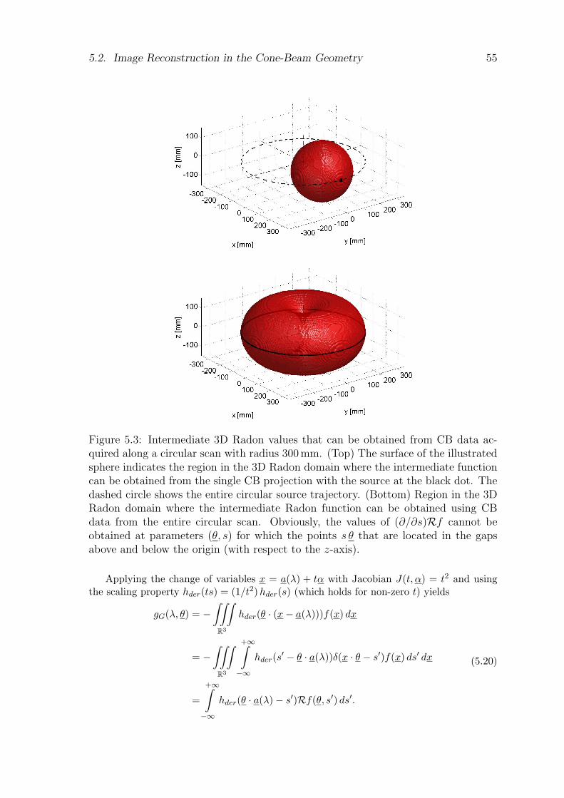
5.2. Image Reconstruction in the Cone-Beam Geometry 55
Figure 5.3: Intermediate 3D Radon values that can be obtained from CB data ac-quired along a circular scan with radius 300mm. (Top) The surface of the illustratedsphere indicates the region in the 3D Radon domain where the intermediate functioncan be obtained from the single CB projection with the source at the black dot. Thedashed circle shows the entire circular source trajectory. (Bottom) Region in the 3DRadon domain where the intermediate Radon function can be obtained using CBdata from the entire circular scan. Obviously, the values of (∂/∂s)Rf cannot beobtained at parameters (θ, s) for which the points s θ that are located in the gapsabove and below the origin (with respect to the z-axis).
Applying the change of variables x = a(λ) + tα with Jacobian J(t, α) = t2 and usingthe scaling property hder(ts) = (1/t2) hder(s) (which holds for non-zero t) yields
gG(λ, θ) = −∫∫∫
R3
hder(θ · (x− a(λ)))f(x) dx
= −∫∫∫
R3
+∞∫
−∞hder(s′ − θ · a(λ))δ(x · θ − s′)f(x) ds′ dx
=
+∞∫
−∞hder(θ · a(λ)− s′)Rf(θ, s′) ds′.
(5.20)
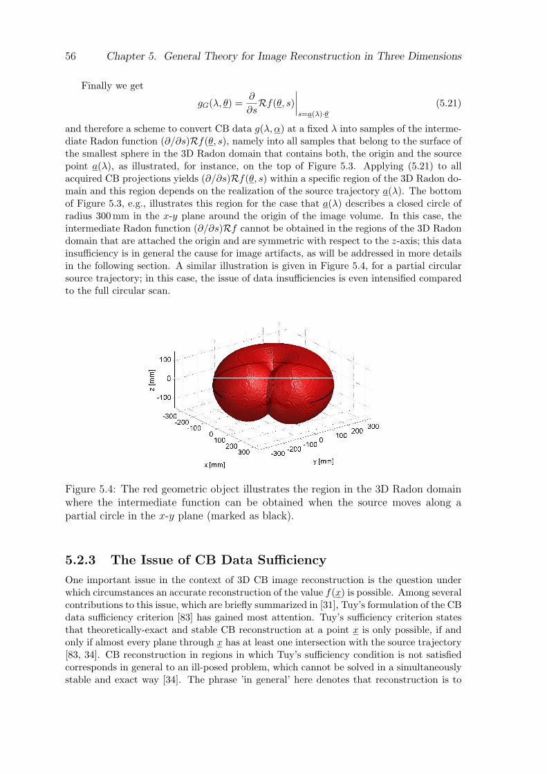
56 Chapter 5. General Theory for Image Reconstruction in Three Dimensions
Finally we get
gG(λ, θ) =∂
∂sRf(θ, s)
∣∣∣∣s=a(λ)·θ
(5.21)
and therefore a scheme to convert CB data g(λ, α) at a fixed λ into samples of the interme-diate Radon function (∂/∂s)Rf(θ, s), namely into all samples that belong to the surface ofthe smallest sphere in the 3D Radon domain that contains both, the origin and the sourcepoint a(λ), as illustrated, for instance, on the top of Figure 5.3. Applying (5.21) to allacquired CB projections yields (∂/∂s)Rf(θ, s) within a specific region of the 3D Radon do-main and this region depends on the realization of the source trajectory a(λ). The bottomof Figure 5.3, e.g., illustrates this region for the case that a(λ) describes a closed circle ofradius 300 mm in the x-y plane around the origin of the image volume. In this case, theintermediate Radon function (∂/∂s)Rf cannot be obtained in the regions of the 3D Radondomain that are attached the origin and are symmetric with respect to the z-axis; this datainsufficiency is in general the cause for image artifacts, as will be addressed in more detailsin the following section. A similar illustration is given in Figure 5.4, for a partial circularsource trajectory; in this case, the issue of data insufficiencies is even intensified comparedto the full circular scan.
Figure 5.4: The red geometric object illustrates the region in the 3D Radon domainwhere the intermediate function can be obtained when the source moves along apartial circle in the x-y plane (marked as black).
5.2.3 The Issue of CB Data Sufficiency
One important issue in the context of 3D CB image reconstruction is the question underwhich circumstances an accurate reconstruction of the value f(x) is possible. Among severalcontributions to this issue, which are briefly summarized in [31], Tuy’s formulation of the CBdata sufficiency criterion [83] has gained most attention. Tuy’s sufficiency criterion statesthat theoretically-exact and stable CB reconstruction at a point x is only possible, if andonly if almost every plane through x has at least one intersection with the source trajectory[83, 34]. CB reconstruction in regions in which Tuy’s sufficiency condition is not satisfiedcorresponds in general to an ill-posed problem, which cannot be solved in a simultaneouslystable and exact way [34]. The phrase ’in general’ here denotes that reconstruction is to
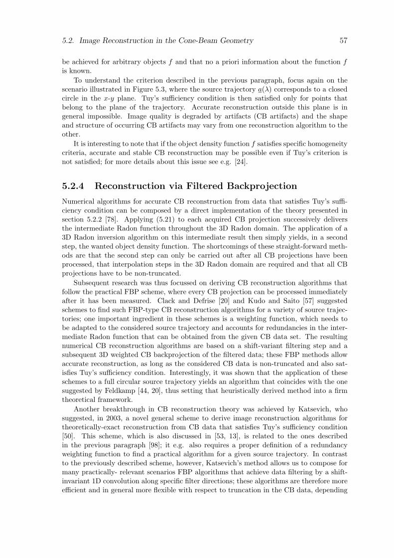
5.2. Image Reconstruction in the Cone-Beam Geometry 57
be achieved for arbitrary objects f and that no a priori information about the function fis known.
To understand the criterion described in the previous paragraph, focus again on thescenario illustrated in Figure 5.3, where the source trajectory a(λ) corresponds to a closedcircle in the x-y plane. Tuy’s sufficiency condition is then satisfied only for points thatbelong to the plane of the trajectory. Accurate reconstruction outside this plane is ingeneral impossible. Image quality is degraded by artifacts (CB artifacts) and the shapeand structure of occurring CB artifacts may vary from one reconstruction algorithm to theother.
It is interesting to note that if the object density function f satisfies specific homogeneitycriteria, accurate and stable CB reconstruction may be possible even if Tuy’s criterion isnot satisfied; for more details about this issue see e.g. [24].
5.2.4 Reconstruction via Filtered Backprojection
Numerical algorithms for accurate CB reconstruction from data that satisfies Tuy’s suffi-ciency condition can be composed by a direct implementation of the theory presented insection 5.2.2 [78]. Applying (5.21) to each acquired CB projection successively deliversthe intermediate Radon function throughout the 3D Radon domain. The application of a3D Radon inversion algorithm on this intermediate result then simply yields, in a secondstep, the wanted object density function. The shortcomings of these straight-forward meth-ods are that the second step can only be carried out after all CB projections have beenprocessed, that interpolation steps in the 3D Radon domain are required and that all CBprojections have to be non-truncated.
Subsequent research was thus focussed on deriving CB reconstruction algorithms thatfollow the practical FBP scheme, where every CB projection can be processed immediatelyafter it has been measured. Clack and Defrise [20] and Kudo and Saito [57] suggestedschemes to find such FBP-type CB reconstruction algorithms for a variety of source trajec-tories; one important ingredient in these schemes is a weighting function, which needs tobe adapted to the considered source trajectory and accounts for redundancies in the inter-mediate Radon function that can be obtained from the given CB data set. The resultingnumerical CB reconstruction algorithms are based on a shift-variant filtering step and asubsequent 3D weighted CB backprojection of the filtered data; these FBP methods allowaccurate reconstruction, as long as the considered CB data is non-truncated and also sat-isfies Tuy’s sufficiency condition. Interestingly, it was shown that the application of theseschemes to a full circular source trajectory yields an algorithm that coincides with the onesuggested by Feldkamp [44, 20], thus setting that heuristically derived method into a firmtheoretical framework.
Another breakthrough in CB reconstruction theory was achieved by Katsevich, whosuggested, in 2003, a novel general scheme to derive image reconstruction algorithms fortheoretically-exact reconstruction from CB data that satisfies Tuy’s sufficiency condition[50]. This scheme, which is also discussed in [53, 13], is related to the ones describedin the previous paragraph [98]; it e.g. also requires a proper definition of a redundancyweighting function to find a practical algorithm for a given source trajectory. In contrastto the previously described scheme, however, Katsevich’s method allows us to compose formany practically- relevant scenarios FBP algorithms that achieve data filtering by a shift-invariant 1D convolution along specific filter directions; these algorithms are therefore moreefficient and in general more flexible with respect to truncation in the CB data, depending
58 Chapter 5. General Theory for Image Reconstruction in Three Dimensions
on the required filter directions. In recent years, a variety of attractive reconstructionalgorithms have been derived from Katsevich’s general theory, such as for instance the onesfor helical source trajectories [49], for circle-plus-arc trajectories [52] or for the ellipse-plus-oblique-line trajectory [25], to name only a few.
5.2.5 Reconstruction via Differentiated Backprojection
As illustrated in the previous section, various FBP methods exist to achieve 3D imagereconstruction from CB data [87]. The common feature of FBP methods is that theyrequire, at some point during CB data filtering, the convolution of data with a filter kernelthat has infinite support. The filtering thus corresponds to a global operation which mayyield inaccurate results in presence of truncation in one or more CB projections.
To tackle this sensitivity with respect to data truncation, novel approaches for CBimage reconstruction have been suggested that avoid the global filtering operation on theprojection data during the filtering step [99, 100, 72]. These approaches first differentiateCB data and then backproject the differentiated data into the image volume to obtain anintermediate function that is linked to the wanted object density function through somefundamental filter relation that involves the Hilbert transform. This relation has beenderived in a general form e.g. in [72]. Reconstruction may then be achieved by transformingthe intermediate function into the function f through additional filtering operations carriedout in the image volume.
Approaches that are based on this scheme are in literature typically known under theterm backprojection-filtration (BPF) or differentiated-backprojection (DBP); they can nat-urally cope with some scenarios of data truncation in which FBP methods fail. More detailsabout these approaches will be given in the following chapters, in the context of circularCB CT.
Chapter 6
Comparative Evaluation of FourCircular Short-ScanReconstruction Methods
6.1 Introduction
Over the past few years, cone-beam X-ray computed tomography has become a powerfulimaging technology in the clinical arena [70, 59]. Among all possible scanning modes,circular motion of the X-ray scanning device relative to the interrogated object remainsone of the most attractive ones. This is because a circular scan is easy to implement,mechanically robust and allows fast data acquisition.
Unfortunately, with the circular as well as with any planar source trajectory, Tuy’sdata sufficiency condition for exact and stable reconstruction [83] is not satisfied for thepoints that lie outside the plane of the X-ray source trajectory, as has been discussedin section 5.2.3. This means that CB image reconstruction is an ill-posed problem almosteverywhere within the image volume [34]; a numerically stable recovery of the object densityfunction in a 3D volume of interest from noisy data can thus only be achieved by sacrificingsome accuracy in the reconstruction result. A reconstruction algorithm can only be usefulfor practical applications if it performs an efficacious trade-off between numerical stabilityand accuracy.
For the closed circular trajectory (full-scan), an attractive algorithm is given by theapproach suggested in 1984 by Feldkamp et al. (FDK) [33]. However, not every X-rayCT system can acquire data along a full-scan. In particular, the mechanical design ofmedical C-arm systems typically prevents data acquisition over more than 330. Moreover,for various physical reasons including dose and scanning time, most scanning protocols onC-arm systems are restricted to a short-scan of 210 to 240 [2]. Hence, FDK cannot beapplied to C-arm systems.
Finding an efficacious algorithm for the short-scan geometry turns out to be a challeng-ing task. A popular algorithm used to achieve image reconstruction in many state-of-the-artC-arm systems is a modification of FDK: short-scan FDK [86]. However, the short-scanFDK method uses geometric approximations to handle data redundancies in the CB dataset and these approximations yield in general a significant amount of CB artifacts in thereconstruction results.
59
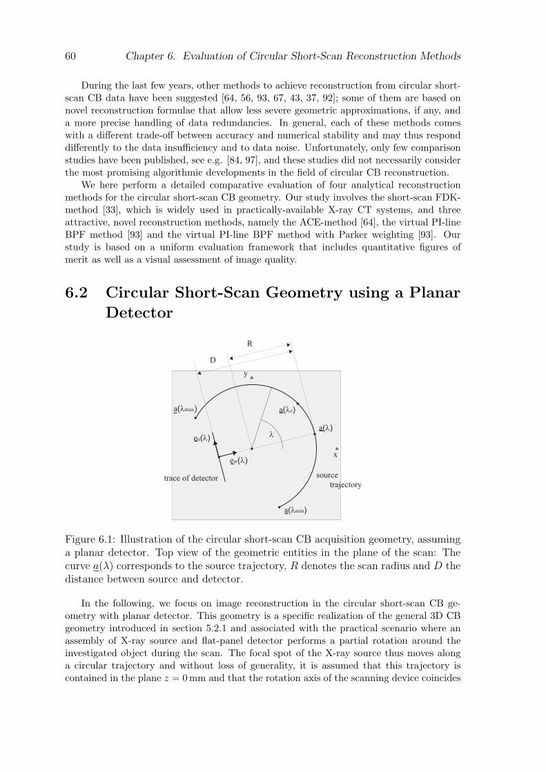
60 Chapter 6. Evaluation of Circular Short-Scan Reconstruction Methods
During the last few years, other methods to achieve reconstruction from circular short-scan CB data have been suggested [64, 56, 93, 67, 43, 37, 92]; some of them are based onnovel reconstruction formulae that allow less severe geometric approximations, if any, anda more precise handling of data redundancies. In general, each of these methods comeswith a different trade-off between accuracy and numerical stability and may thus responddifferently to the data insufficiency and to data noise. Unfortunately, only few comparisonstudies have been published, see e.g. [84, 97], and these studies did not necessarily considerthe most promising algorithmic developments in the field of circular CB reconstruction.
We here perform a detailed comparative evaluation of four analytical reconstructionmethods for the circular short-scan CB geometry. Our study involves the short-scan FDK-method [33], which is widely used in practically-available X-ray CT systems, and threeattractive, novel reconstruction methods, namely the ACE-method [64], the virtual PI-lineBPF method [93] and the virtual PI-line BPF method with Parker weighting [93]. Ourstudy is based on a uniform evaluation framework that includes quantitative figures ofmerit as well as a visual assessment of image quality.
6.2 Circular Short-Scan Geometry using a Planar
Detector
Figure 6.1: Illustration of the circular short-scan CB acquisition geometry, assuminga planar detector. Top view of the geometric entities in the plane of the scan: Thecurve a(λ) corresponds to the source trajectory, R denotes the scan radius and D thedistance between source and detector.
In the following, we focus on image reconstruction in the circular short-scan CB ge-ometry with planar detector. This geometry is a specific realization of the general 3D CBgeometry introduced in section 5.2.1 and associated with the practical scenario where anassembly of X-ray source and flat-panel detector performs a partial rotation around theinvestigated object during the scan. The focal spot of the X-ray source thus moves alonga circular trajectory and without loss of generality, it is assumed that this trajectory iscontained in the plane z = 0 mm and that the rotation axis of the scanning device coincides
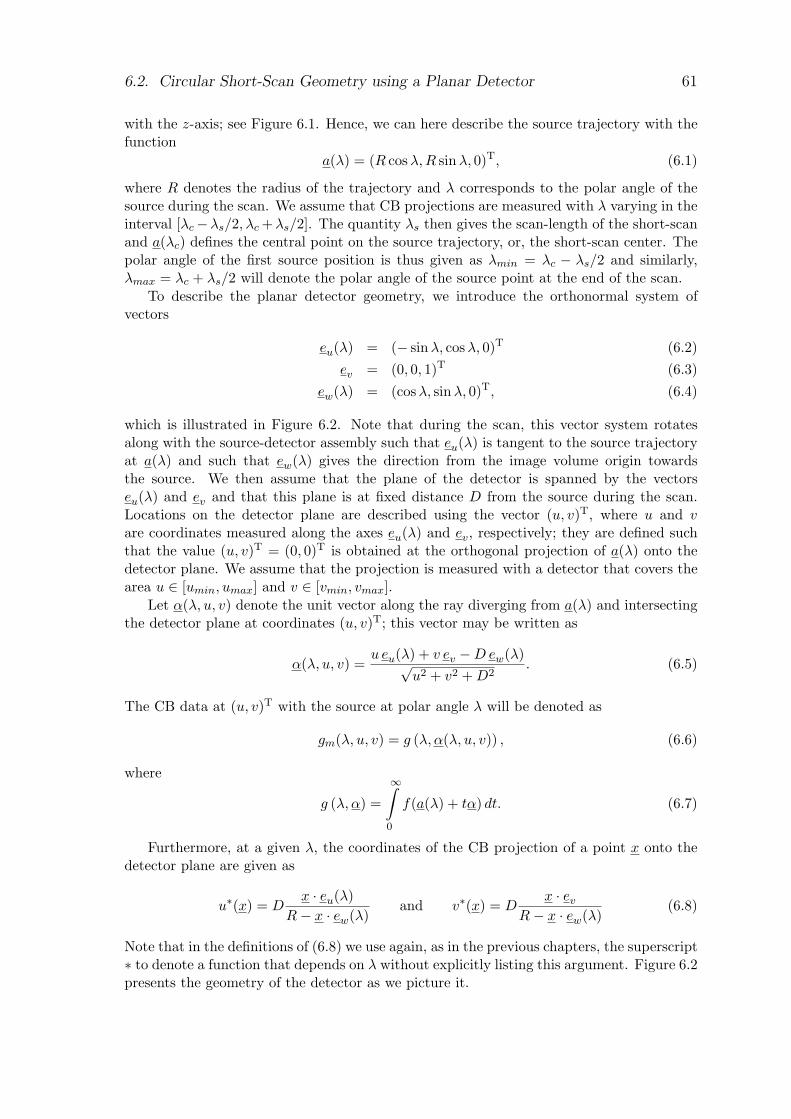
6.2. Circular Short-Scan Geometry using a Planar Detector 61
with the z-axis; see Figure 6.1. Hence, we can here describe the source trajectory with thefunction
a(λ) = (R cosλ,R sinλ, 0)T, (6.1)
where R denotes the radius of the trajectory and λ corresponds to the polar angle of thesource during the scan. We assume that CB projections are measured with λ varying in theinterval [λc−λs/2, λc +λs/2]. The quantity λs then gives the scan-length of the short-scanand a(λc) defines the central point on the source trajectory, or, the short-scan center. Thepolar angle of the first source position is thus given as λmin = λc − λs/2 and similarly,λmax = λc + λs/2 will denote the polar angle of the source point at the end of the scan.
To describe the planar detector geometry, we introduce the orthonormal system ofvectors
eu(λ) = (− sinλ, cosλ, 0)T (6.2)ev = (0, 0, 1)T (6.3)
ew(λ) = (cosλ, sinλ, 0)T, (6.4)
which is illustrated in Figure 6.2. Note that during the scan, this vector system rotatesalong with the source-detector assembly such that eu(λ) is tangent to the source trajectoryat a(λ) and such that ew(λ) gives the direction from the image volume origin towardsthe source. We then assume that the plane of the detector is spanned by the vectorseu(λ) and ev and that this plane is at fixed distance D from the source during the scan.Locations on the detector plane are described using the vector (u, v)T, where u and vare coordinates measured along the axes eu(λ) and ev, respectively; they are defined suchthat the value (u, v)T = (0, 0)T is obtained at the orthogonal projection of a(λ) onto thedetector plane. We assume that the projection is measured with a detector that covers thearea u ∈ [umin, umax] and v ∈ [vmin, vmax].
Let α(λ, u, v) denote the unit vector along the ray diverging from a(λ) and intersectingthe detector plane at coordinates (u, v)T; this vector may be written as
α(λ, u, v) =u eu(λ) + v ev −D ew(λ)√
u2 + v2 + D2. (6.5)
The CB data at (u, v)T with the source at polar angle λ will be denoted as
gm(λ, u, v) = g (λ, α(λ, u, v)) , (6.6)
where
g (λ, α) =
∞∫
0
f(a(λ) + tα) dt. (6.7)
Furthermore, at a given λ, the coordinates of the CB projection of a point x onto thedetector plane are given as
u∗(x) = Dx · eu(λ)
R− x · ew(λ)and v∗(x) = D
x · ev
R− x · ew(λ)(6.8)
Note that in the definitions of (6.8) we use again, as in the previous chapters, the superscript∗ to denote a function that depends on λ without explicitly listing this argument. Figure 6.2presents the geometry of the detector as we picture it.
62 Chapter 6. Evaluation of Circular Short-Scan Reconstruction Methods
Figure 6.2: Geometric entities associated with the planar detector. The quantitiesumin, umax, vmin and vmax define the detector size, and u∗(x) and v∗(x) are thecoordinates of the CB projection of x onto the detector plane.
If the CB projection of the object lies within the measured detector area for each λ,i.e., if u∗(x) ∈ [umin, umax] and v∗(x) ∈ [vmin, vmax] for all x ∈ Ωf and all λ ∈ [λmin, λmax],CB data will be called non-truncated. If the projection of the object exceeds the measuredinterval in u for some λ, the CB data suffers from transaxial truncation. On the other hand,if this projection exceeds the measured interval in v, we say that the CB data set containsaxial truncation.
Image reconstruction in the circular short-scan CB geometry then refers to the taskof recovering the object density function f(x) for x ∈ Ωf from the measured CB datagm(λ, u, v) with λ ∈ [λmin, λmax], u ∈ [umin, umax] and v ∈ [vmin, vmax]. Since this taskcannot be simultaneously solved in a theoretically-exact and in a stable way and sincediscretization impacts the numerical computation, we can in general only compute an ap-proximate estimate fe(x) of the true object density function. The following sections presentfour state-of-the-art methods that have been suggested in the literature to compute suchan estimate.
6.3 The Short-Scan FDK Method
The short-scan FDK method is based on the algorithm introduced in 1984 by Feldkamp,Davis and Kress (FDK) [33] for approximate reconstruction from CB data acquired alonga full circular scan (i.e., for a scan with λs = 360). The full-scan FDK reconstructionalgorithm is well-understood in terms of the 3D Radon theory [20, 57]. Almost all 3D Radonplanes through Ωf intersect the full circular source trajectory either twice or never. Thefull-scan FDK method uses for reconstruction the information associated with 3D Radonplanes that have two such intersections. It weights each data sample with a factor of 1/2resulting in an equal contribution of every used 3D Radon value to the final reconstruction.Data associated to 3D Radon planes that do not intersect the source trajectory is never
6.3. The Short-Scan FDK Method 63
measured and does not contribute to the FDK estimation of the object density; this lackof information causes CB artifacts in the reconstruction result.
In the short-scan geometry, the distribution of data redundancies is more complex - some3D Radon planes intersect the source trajectory once, others twice, others never. Thus, thebeneficial Radon-plane based weighting scheme intrinsically used for the full-scan trajectorythat weights every measurement with 1/2 cannot be applied. Wang et al. [86] suggestedan heuristic modification of the full-scan FDK reconstruction approach to be able to applythat method for reconstruction from CB data corresponding to a circular short-scan. In thismodification, which we will refer to as the short-scan FDK method from now on, CB data ismultiplied with a v-independent weighing function prior to reconstruction to approximatelyaccount for data redundancies. A common selection for the weighting function, which weuse within this comparison study, is the generalized Parker weighting function [79] that wasintroduced in chapter 3.2.3.
6.3.1 Reconstruction Method
The short-scan FDK method computes an estimate fe of the object density function f fromthe circular CB data using the following steps:
Step 1 – Weighting: CB data is multiplied with a length correction weight and with theredundancy function to yield weighted CB projections
gw(λ, u, v) =D√
u2 + v2 + D2mgp(λ, u) gm(λ, u, v) (6.9)
where
mgp(λ, u) = m(λ, tan
u
D
)(6.10)
gives the generalized Parker weighting function [79] for the flat panel geometry; see(3.48) on page 26 for a definition.
Step 2 – 1D Filtering: Convolution of the weighted CB projections in u with the kernelof the ramp filter yields filtered CB projections denoted as
gF (λ, u, v) =
umax∫
umin
hramp(u− u′)gw(λ, u′, v) du′. (6.11)
Step 3 – 3D Backprojection: Filtered CB projections are backprojected into the imagevolume using the entire acquired interval in λ to yield the object estimate
fe(x) = RD
λmax∫
λmin
gF (λ, u∗(x), v∗(x))(R− x · ew(λ))2
dλ (6.12)
with functions u∗ and v∗ defined in (6.8).
64 Chapter 6. Evaluation of Circular Short-Scan Reconstruction Methods
6.3.2 Implementation Details
The short-scan FDK method follows the FBP scheme and involves only 1D filtering alonglines that are in the direction of eu(λ); it is thus relatively easy to implement and compu-tationally efficient. The numerical algorithm considered in this evaluation study achieveddata filtering and weighting by discretizing equations (6.9) and (6.11) at k∆u with k ∈ Z,and therefore yields the filter result on a sampling grid in u and v that is identical to thatof the initial CB data function gm. For implementation of (6.11) we used a band-limitedversion of the ramp filter kernel with bandwidth set to 1/(2∆u) and furthermore usedsinc apodization on the kernel. To increase computation speed, the convolution in (6.11)was carried out in frequency domain, using standard signal-processing techniques. 3D CBbackprojection according to (6.12) was implemented by approximating the integral in thisequation with a discrete sum according to the rectangular rule of numerical integration andby using bilinear interpolation in u and v to obtain in each filtered CB projection the valuesrequired at u∗(x) and v∗(x).
6.4 The ACE Method
In 2003, Katsevich presented a novel, general framework to construct theoretically-exactinversion formulae for the 3D divergent beam transform for a large class of source trajec-tories [50]; see section 5.2.4. Reconstruction at a specific point x using such a formula canyield accurate results, dependent on the actual degree of data truncation, if the CB dataset satisfies Tuy’s sufficiency condition for exact and stable reconstruction at x. The ACEmethod [64] (the acronym stands for arc based cone-beam reconstruction using an equal-weighting scheme) has been derived by applying Katsevich’s framework to the short-scancircular source trajectory and by intrinsically using a uniform weighting of the measured 3DRadon data, following principles already applied in [67]. Hence, data redundancies in theCB data are handled accurately rather than by using a heuristic weighting scheme. How-ever, CB data collected along the circular trajectory satisfies Tuy’s sufficiency conditiononly for points inside the plane of the source motion. Hence, the ACE method will yieldaccurate results only within the slice z = 0 and will in general yield approximate resultseverywhere else throughout the image volume.
6.4.1 Reconstruction Method
The ACE method computes an estimate fe of the object density function from the knownCB data as follows:
Step 1 – Differentiation: Differentiation of CB data in λ at fixed ray direction yieldsdifferentiated CB projections denoted as
gd(λ, u, v) = limε→0
g (λ + ε, α(λ, u, v))− g (λ− ε, α(λ, u, v))2ε
(6.13)
Step 2 – Weighting: Cosine weighting of the differentiated CB data yields
gw(λ, u, v) =D√
u2 + v2 + D2gd(λ, u, v). (6.14)
6.4. The ACE Method 65
Step 3 – 1D Filtering: The weighted and differentiated CB data is convolved with thekernel of the Hilbert transform along 3 filtering lines to yield 3 filtered CB projections:
gF1(λ, u, v) =
umax∫
umin
hhilb(u− u′)gw(λ, u′, v) du′, (6.15)
gF2(λ, u, v) =
umax∫
umin
hhilb(u− u′)gw(λ, u′, v′1(λ, u, u′, v)) du′, (6.16)
gF3(λ, u, v) =
umax∫
umin
hhilb(u− u′)gw(λ, u′, v′2(λ, u, u′, v)) du′, (6.17)
with v′1 and v′2 denoting the equations of two lines on the detector plane:
v′1(λ, u, u′, v) = v + (u− u′)κ1, κ1 =v − v∗(a(λmin))u− u∗(a(λmin))
, (6.18)
v′2(λ, u, u′, v) = v + (u− u′)κ2, κ2 =v − v∗(a(λmax))u− u∗(a(λmax))
(6.19)
and κ1 and κ2 denoting their respective slopes.
The computation of one filter sample according to (6.15) requires function gw at fixedv; filtering is therefore geometrically carried out along filter lines on the detector thatare parallel to the u-axis, as in the FDK method. The convolutions in (6.16) and(6.17), however, involve values of gw on filter lines that vary with λ and are in generaloblique. More specifically, to obtain at a given λ the function gF2 at point (u, v)T,consider the line that connects this point with the CB projection of the first sourceposition a(λmin) onto the detector plane; the equation of this line is given by (6.18).The desired value of gF2 is then obtained by convolving values of gw along this linewith the kernel of the Hilbert transform and evaluating the convolution result atcoordinate u. Data filtering for gF3 follows a similar scheme; it requires filter linesthat contain the CB projection of a(λmax) onto the detector plane, the equations ofwhich are given by (6.19).
Step 4 – 3D Backprojection: The ACE estimate of the object density function is ob-tained by 3D backprojection of the filtered CB projections using a non-squared back-projection weight, according to
fe(x) = − 14π2
λmax∫
λmin
1R− x · ew(λ)
(gF1(λ, u∗(x), v∗(x))
+sign (u∗(x)− u∗(a(λmin)))
2gF2 (λ, u∗(x), v∗(x))
+sign (u∗(a(λmax))− u∗(x))
2gF3 (λ, u∗(x), v∗(x))
)dλ
(6.20)
6.4.2 Implementation Details
As the short-scan FDK method, the ACE algorithm also uses the FBP scheme, but ACEinvolves a filtering step that is more complex than that of FDK: it requires CB data dif-ferentiation, data weighting and three different 1D convolutions with the Hilbert kernel.
66 Chapter 6. Evaluation of Circular Short-Scan Reconstruction Methods
The differentiation of CB data according to (6.13) was here implemented following theview-differentiation scheme described in [68]. This scheme requires the selection of a differ-entiation parameter, which plays a similar role than ε in (6.13). We here fix this parameterto ε = 0.01, because this specific value was found to yield both, good spatial resolution inthe differentiation result and good numerical stability [68].
Hilbert filtering was achieved by discretizing (6.15)-(6.17) at coordinates k∆u 1 and byreplacing the Hilbert kernel with its band-limited version, using rectangular apodization andbandwidth 1/(2∆u). Computationally efficient filtering along non-horizonal lines, whichoccur in (6.16) and (6.17), was achieved using an approach similar to that explained in [69].First, the slope parameters κ1 and κ2 were discretized, which geometrically means that datafiltering involved a fixed number of filtering lines. The discretization steps ∆κ1 and ∆κ2
were selected in a way that the v-coordinates of the intersection of the axis u = 0 with anytwo neighboring filter lines differed by ∆v/2. Note that this scheme yielded a number offilter lines used for computation of g2 or g3 that is twice as high as the number of filter linesused for term g1. Next, values of gw along these filter lines were extracted, in a so calledforward-rebinning step, using linear interpolation in v. These values were then convolvedwith the Hilbert kernel and subsequently, in a back-rebinning step, transformed back on aCartesian sampling grid in u and v. This back-rebinning involved bilinear interpolation andwas carried out on a sampling pattern with 8 times finer sampling along each dimensioncompared to the initial grid on which the function gw is known.
3D CB backprojection was carried out by first combining the three filter contributionson the upsampled grid and then using nearest neighbor interpolation in u and v to obtainthe required samples at u∗(x) and v∗(x) from this combined filter result.
6.5 The Virtual PI-Line BPF Methods
The third and forth reconstruction methods used in this comparison study are based on atheoretically exact reconstruction formula that has been proposed for image reconstructionfrom CB data acquired along a helical source trajectory [100]. The helical reconstructionformula described in this reference follows a scheme that the authors of [100] refer to asbackprojection-filtration (BPF): Reconstruction is achieved by first backprojecting differen-tiated CB data into the image volume and then using 1D filtering along PI-lines to convertthe backprojection result into the object density estimate; here, a PI-line is a line that con-nects two points on the source trajectory. An important feature of the BPF methods is thatthey naturally allow in some scenarios accurate reconstruction from transaxially-truncatedCB data, in contrast to the FBP methods described earlier in this chapter [100, 99, 72].
In [93], the helical reconstruction formula has been modified to be useful for 3D recon-struction from a circular short-scan. Obviously, in this geometry, PI-lines only exist in theplane of the source motion; to allow reconstruction in other regions of the image volume, socalled virtual PI-lines are heuristically introduced that are parallel to the plane z = 0mm.The resulting reconstruction method will be denoted as the virtual PI-Line BPF methodfrom now on.
1Note that filter lines with slopes of magnitude exceeding 1 were handled differently: equations(6.16) and (6.17) were then expressed as a convolution with respect to v instead of with respect to u.This yields a finer sampling on very oblique filter lines and thus less aliasing and better performancein the discrete scenario [64].
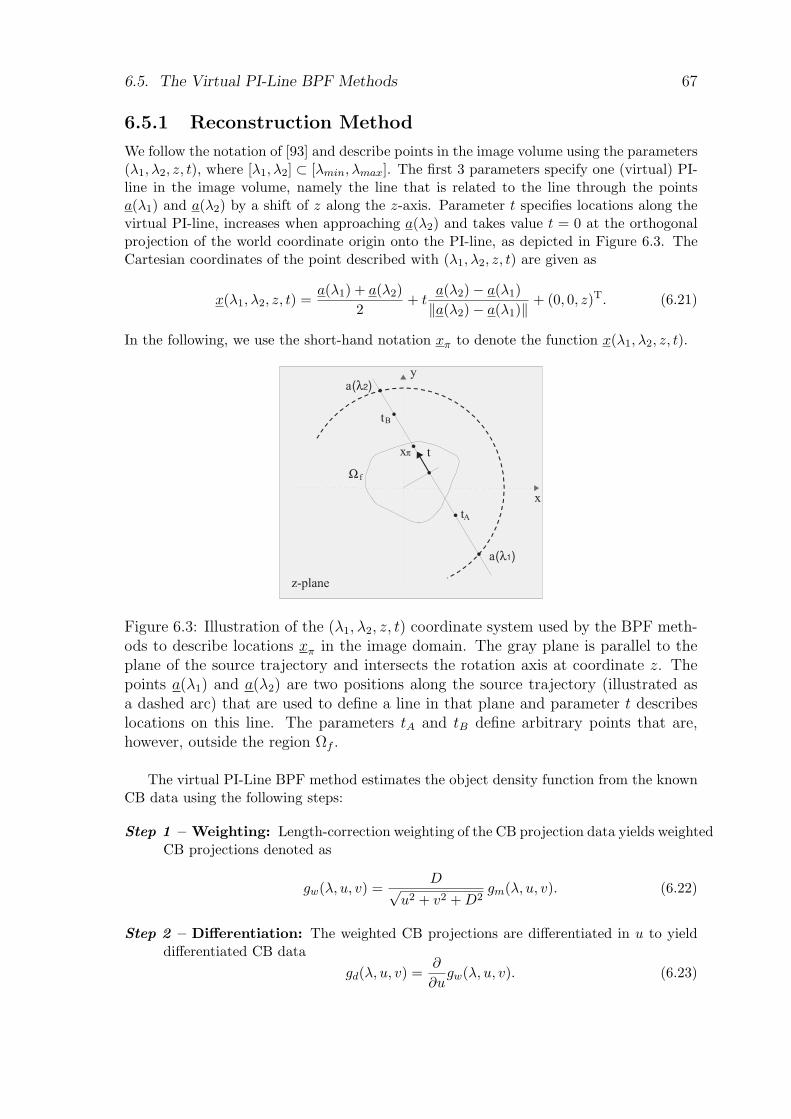
6.5. The Virtual PI-Line BPF Methods 67
6.5.1 Reconstruction Method
We follow the notation of [93] and describe points in the image volume using the parameters(λ1, λ2, z, t), where [λ1, λ2] ⊂ [λmin, λmax]. The first 3 parameters specify one (virtual) PI-line in the image volume, namely the line that is related to the line through the pointsa(λ1) and a(λ2) by a shift of z along the z-axis. Parameter t specifies locations along thevirtual PI-line, increases when approaching a(λ2) and takes value t = 0 at the orthogonalprojection of the world coordinate origin onto the PI-line, as depicted in Figure 6.3. TheCartesian coordinates of the point described with (λ1, λ2, z, t) are given as
x(λ1, λ2, z, t) =a(λ1) + a(λ2)
2+ t
a(λ2)− a(λ1)‖a(λ2)− a(λ1)‖ + (0, 0, z)T. (6.21)
In the following, we use the short-hand notation xπ to denote the function x(λ1, λ2, z, t).
y
tA
a
z-plane
B
f
a
x
x
t
t
Figure 6.3: Illustration of the (λ1, λ2, z, t) coordinate system used by the BPF meth-ods to describe locations xπ in the image domain. The gray plane is parallel to theplane of the source trajectory and intersects the rotation axis at coordinate z. Thepoints a(λ1) and a(λ2) are two positions along the source trajectory (illustrated asa dashed arc) that are used to define a line in that plane and parameter t describeslocations on this line. The parameters tA and tB define arbitrary points that are,however, outside the region Ωf .
The virtual PI-Line BPF method estimates the object density function from the knownCB data using the following steps:
Step 1 – Weighting: Length-correction weighting of the CB projection data yields weightedCB projections denoted as
gw(λ, u, v) =D√
u2 + v2 + D2gm(λ, u, v). (6.22)
Step 2 – Differentiation: The weighted CB projections are differentiated in u to yielddifferentiated CB data
gd(λ, u, v) =∂
∂ugw(λ, u, v). (6.23)
68 Chapter 6. Evaluation of Circular Short-Scan Reconstruction Methods
Step 3 – 3D Backprojection: Backprojection of the differentiated CB projections usingonly the interval in λ ∈ [λ1, λ2] and backprojection of boundary terms at λ1 and λ2
yields an intermediate function in the image domain
f(λ1, λ2, z, t) = DR
λ2∫
λ1
gd(λ, u∗(xπ), v∗(xπ))(R− xπ · ew(λ))2
dλ
+gm(λ, u∗(xπ), v∗(xπ))
‖xπ − a(λ)‖
∣∣∣∣λ2
λ1
(6.24)
with functions u∗ and v∗ defined in (6.8).
Step 4 – 1D Filtering: The object density estimate is obtained from the intermediatefunction through 1D filtering
fe(xπ) =12π
1√(tB − t)(t− tA)
×
tB∫
tA
hhilb(t− t′)√
(tB − t)(t− tA)f(λ1, λ2, z, t′)dt′ + 2P
.
(6.25)
The quantities tA and tB > tA are coordinates along the virtual PI-Line containingxπ that describe points that are outside and on opposite sides of the object supportregion Ωf . The term 2P in (6.25) stands for
2P = gm (λ, u∗(xπ), v∗(xπ))∣∣∣∣t=0,λ=λ1
+ gm (λ, u∗(xπ), v∗(xπ))∣∣∣∣t=0,λ=λ2
(6.26)
i.e., 2P is the sum of the CB data samples corresponding to the rays that divergefrom a(λ1) or a(λ2) and contain the central point on the virtual PI line, at coordinatet = 0, as suggested in [93].
6.5.2 The Virtual PI-Line BPF Method with Parker Weight-ing
The virtual PI-Line reconstruction method explained above uses for reconstruction onlythe CB data corresponding to λ ∈ [λ1, λ2]. To consider all acquired CB projections forreconstruction, a modification of the algorithm explained above has been suggested [93]that differs from that algorithm as follows:
Difference 1 – Weighting: CB data weighting now also involves a multiplication witha weighting function that is designed to approximately account for redundancies inthe CB data for λ ∈ [λ1, λ2]. This approach is identical to that used in the short-scan FDK method; a popular choice is again to use the generalized Parker weightingfunction, defined in (6.10), so that altogether, we obtain weighted CB projections as
gw(λ, u, v) =D√
u2 + v2 + D2mgp(λ, u) gm(λ, u, v). (6.27)
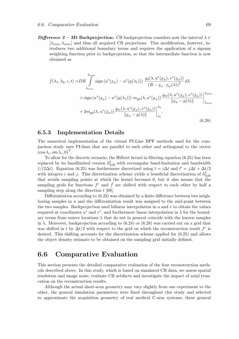
6.6. Comparative Evaluation 69
Difference 2 – 3D Backprojection: CB backprojection considers now the interval λ ∈[λmin, λmax] and thus all acquired CB projections. This modification, however, in-troduces two additional boundary terms and requires the application of a signumweighting function prior to backprojection, so that the intermediate function is nowobtained as
f(λ1, λ2, z, t) =DR
λmax∫
λmin
sign (u∗(xπ)− u∗(a(λ1)))gd(λ, u∗(xπ), v∗(xπ))
(R− xπ · ew(λ))2dλ
+ sign (u∗(xπ)− u∗(a(λ1))) mgp(λ, u∗(xπ))gm(λ, u∗(xπ), v∗(xπ))
‖xπ − a(λ)‖
∣∣∣∣λmax
λmin
+ 2mgp(λ, u∗(xπ))gm(λ, u∗(xπ), v∗(xπ))
‖xπ − a(λ)‖
∣∣∣∣λ2
λ1
.
(6.28)
6.5.3 Implementation Details
The numerical implementation of the virtual PI-Line BPF methods used for the com-parison study uses PI-lines that are parallel to each other and orthogonal to the vector(cosλc, sinλc, 0)T.
To allow for the discrete scenario, the Hilbert kernel in filtering equation (6.25) has beenreplaced by its bandlimited version hb
hilb with rectangular band-limitation and bandwidth1/(2∆t). Equation (6.25) was furthermore discretized using t = i∆t and t′ = j∆t + ∆t/2with integers i and j. This discretization scheme yields a beneficial discretization of hb
hilb
that avoids sampling points at which the kernel becomes 0, but it also means that thesampling grids for functions fe and f are shifted with respect to each other by half asampling step along the direction t [69].
Differentiation according to (6.23) was obtained by a finite difference between two neigh-boring samples in u and the differentiation result was assigned to the mid-point betweenthe two samples. Backprojection used bilinear interpolation in u and v to obtain the valuesrequired at coordinates u∗ and v∗, and furthermore linear interpolation in λ for the bound-ary terms from source locations λ that do not in general coincide with the known samplesin λ. Moreover, backprojection according to (6.24) or (6.28) was carried out on a grid thatwas shifted in t by ∆t/2 with respect to the grid on which the reconstruction result fe isdesired. This shifting accounts for the discretization scheme applied for (6.25) and allowsthe object density estimate to be obtained on the sampling grid initially defined.
6.6 Comparative Evaluation
This section presents the detailed comparative evaluation of the four reconstruction meth-ods described above. In this study, which is based on simulated CB data, we assess spatialresolution and image noise, evaluate CB artifacts and investigate the impact of axial trun-cation on the reconstruction results.
Although the actual short-scan geometry may vary slightly from one experiment to theother, the general simulation parameters were fixed throughout this study and selectedto approximate the acquisition geometry of real medical C-arm systems; these general
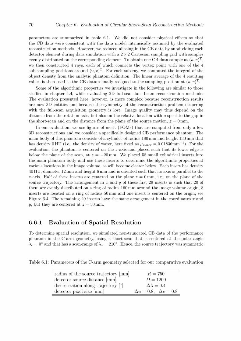
70 Chapter 6. Evaluation of Circular Short-Scan Reconstruction Methods
parameters are summarized in table 6.1. We did not consider physical effects so thatthe CB data were consistent with the data model intrinsically assumed by the evaluatedreconstruction methods. However, we reduced aliasing in the CB data by subdividing eachdetector element during data simulation with a 2× 2 Cartesian sampling grid with samplesevenly distributed on the corresponding element. To obtain one CB data sample at (u, v)T,we then constructed 4 rays, each of which connects the vertex point with one of the 4sub-sampling positions around (u, v)T. For each sub-ray, we computed the integral of theobject density from the analytic phantom definition. The linear average of the 4 resultingvalues is then used as the CB datum finally assigned to the sampling position at (u, v)T.
Some of the algorithmic properties we investigate in the following are similar to thosestudied in chapter 4.4, while evaluating 2D full-scan fan- beam reconstruction methods.The evaluation presented here, however, is more complex because reconstruction resultsare now 3D entities and because the symmetry of the reconstruction problem occurringwith the full-scan acquisition geometry is lost. Image quality may thus depend on thedistance from the rotation axis, but also on the relative location with respect to the gap inthe short-scan and on the distance from the plane of the source motion, z = 0 mm.
In our evaluation, we use figures-of-merit (FOMs) that are computed from only a few3D reconstructions and we consider a specifically designed CB performance phantom. Themain body of this phantom consists of a cylinder of radius 180 mm and height 130 mm thathas density 0HU (i.e., the density of water, here fixed as µwater = 0.01836mm−1). For theevaluation, the phantom is centered on the z-axis and placed such that its lower edge isbelow the plane of the scan, at z = −20 mm. We placed 58 small cylindrical inserts intothe main phantom body and use these inserts to determine the algorithmic properties atvarious locations in the image volume, as will become clearer below. Each insert has density40HU, diameter 12 mm and height 6 mm and is oriented such that its axis is parallel to thez-axis. Half of these inserts are centered on the plane z = 0 mm, i.e., on the plane of thesource trajectory. The arrangement in x and y of these first 29 inserts is such that 20 ofthem are evenly distributed on a ring of radius 160 mm around the image volume origin, 8inserts are located on a ring of radius 50 mm and one insert is centered on the origin; seeFigure 6.4. The remaining 29 inserts have the same arrangement in the coordinates x andy, but they are centered at z = 50 mm.
6.6.1 Evaluation of Spatial Resolution
To determine spatial resolution, we simulated non-truncated CB data of the performancephantom in the C-arm geometry, using a short-scan that is centered at the polar angleλc = 0 and that has a scan-range of λs = 210. Hence, the source trajectory was symmetric
Table 6.1: Parameters of the C-arm geometry selected for our comparative evaluation
radius of the source trajectory [mm] R = 750detector-source distance [mm] D = 1200discretization along trajectory [] ∆λ = 0.4detector pixel size [mm] ∆u = 0.8, ∆v = 0.8
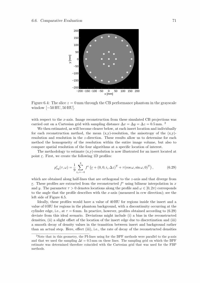
6.6. Comparative Evaluation 71
x [mm]
y [m
m]
−200 −150 −100 −50 0 50 100 150 200−200
−150
−100
−50
0
50
100
150
200
Figure 6.4: The slice z = 0mm through the CB performance phantom in the grayscalewindow [−50 HU, 50 HU].
with respect to the x-axis. Image reconstruction from these simulated CB projections wascarried out on a Cartesian grid with sampling distance ∆x = ∆y = ∆z = 0.5mm. 2
We then estimated, as will become clearer below, at each insert location and individuallyfor each reconstruction method, the mean (x,y)-resolution, the anisotropy of the (x,y)-resolution and resolution in the z-direction. These results allow us to determine for eachmethod the homogeneity of the resolution within the entire image volume, but also tocompare spatial resolution of the four algorithms at a specific location of interest.
The methodology to estimate (x,y)-resolution is now illustrated for an insert located atpoint r. First, we create the following 1D profiles:
pexy(τ, ω) =
19
4∑
iz=−4
fe(r + (0, 0, iz ∆z)T + τ(cosω, sinω, 0)T
), (6.29)
which are obtained along half-lines that are orthogonal to the z-axis and that diverge fromr. These profiles are extracted from the reconstructed fe using bilinear interpolation in xand y. The parameter τ > 0 denotes locations along the profile and ω ∈ [0, 2π) correspondsto the angle that the profile describes with the x-axis (measured in ccw direction); see theleft side of Figure 6.5.
Ideally, these profiles would have a value of 40HU for regions inside the insert and avalue of 0HU for regions in the phantom background, with a discontinuity occurring at thecylinder edge, i.e., at τ = 6mm. In practice, however, profiles obtained according to (6.29)deviate from this ideal scenario. Deviations might include (i) a bias in the reconstructeddensities, (ii) a slight offset of the location of the insert edge due to discretization and (iii)a smooth decay of density values in the transition between insert and background ratherthan an actual step. Here, effect (iii), i.e., the rate of decay of the reconstructed densities
2Note that in this geometry, the PI-lines using for the BPF methods were parallel to the y-axisand that we used the sampling ∆t = 0.5mm on these lines. The sampling grid on which the BPFestimate was determined therefore coincided with the Cartesian grid that was used for the FBPmethods.
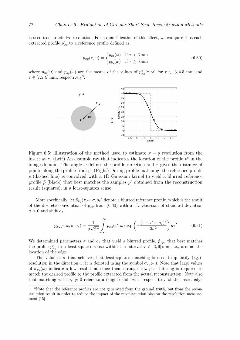
72 Chapter 6. Evaluation of Circular Short-Scan Reconstruction Methods
is used to characterize resolution. For a quantification of this effect, we compare thus eachextracted profile pe
xy to a reference profile defined as
pxy(τ, ω) =
pin(ω) if τ < 6mmpbg(ω) if τ ≥ 6mm
(6.30)
where pin(ω) and pbg(ω) are the means of the values of pexy(τ, ω) for τ ∈ [3, 4.5]mm and
τ ∈ [7.5, 9]mm, respectively3.
4.5 5 5.5 6 6.5 7 7.5−5
0
5
10
15
20
25
30
35
40
45
t [mm]
dens
ity [H
U]
Figure 6.5: Illustration of the method used to estimate x − y resolution from theinsert at r. (Left) An example ray that indicates the location of the profile pe in theimage domain. The angle ω defines the profile direction and τ gives the distance ofpoints along the profile from r. (Right) During profile matching, the reference profilep (dashed line) is convolved with a 1D Gaussian kernel to yield a blurred referenceprofile p (black) that best matches the samples pe obtained from the reconstructionresult (squares), in a least-squares sense.
More specifically, let pxy(τ, ω, σ, oτ ) denote a blurred reference profile, which is the resultof the discrete convolution of pxy from (6.30) with a 1D Gaussian of standard deviationσ > 0 and shift oτ :
pxy(τ, ω, σ, oτ ) =1
σ√
2π
∞∫
−∞pxy(τ ′, ω) exp
(−(τ − τ ′ + oτ )2
2σ2
)dτ ′ (6.31)
We determined parameters σ and oτ that yield a blurred profile, pxy, that best matchesthe profile pe
xy in a least-squares sense within the interval τ ∈ [3, 9]mm, i.e., around thelocation of the edge.
The value of σ that achieves that least-squares matching is used to quantify (x,y)-resolution in the direction ω; it is denoted using the symbol σxy(ω). Note that large valuesof σxy(ω) indicate a low resolution, since then, stronger low-pass filtering is required tomatch the desired profile to the profile extracted from the actual reconstruction. Note alsothat matching with oτ 6= 0 refers to a (slight) shift with respect to τ of the insert edge
3Note that the reference profiles are not generated from the ground truth, but from the recon-struction result in order to reduce the impact of the reconstruction bias on the resolution measure-ment [15]
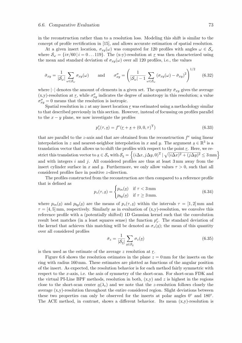
6.6. Comparative Evaluation 73
in the reconstruction rather than to a resolution loss. Modeling this shift is similar to theconcept of profile rectification in [15], and allows accurate estimation of spatial resolution.
At a given insert location, σxy(ω) was computed for 120 profiles with angles ω ∈ Sω
where Sω = iπ/60 | i = 0 . . . 119. The (x-y)-resolution at r was then characterized usingthe mean and standard deviation of σxy(ω) over all 120 profiles, i.e., the values
σxy =1|Sω|
∑
ω∈Sω
σxy(ω) and σσxy =
(1
|Sω| − 1
∑
ω∈Sω
(σxy(ω)− σxy)2
)1/2
(6.32)
where | · | denotes the amount of elements in a given set. The quantity σxy gives the average(x,y)-resolution at r, while σσ
xy indicates the degree of anisotropy in this resolution; a valueσσ
xy = 0 means that the resolution is isotropic.Spatial resolution in z at any insert location r was estimated using a methodology similar
to that described previously in this section. However, instead of focussing on profiles parallelto the x− y plane, we now investigate the profiles
pez(τ, s) = fe(r + s + (0, 0, τ)T) (6.33)
that are parallel to the z-axis and that are obtained from the reconstruction fe using linearinterpolation in z and nearest-neighbor interpolation in x and y. The argument s ∈ R3 is atranslation vector that allows us to shift the profiles with respect to the point r. Here, we re-strict this translation vector to s ∈ Ss with Ss =
(i∆x, j∆y, 0)T |
√(i∆x)2 + (j∆y)2 ≤ 3mm
and with integers i and j. All considered profiles are thus at least 3mm away from theinsert cylinder surface in x and y. Furthermore, we only allow values τ > 0, such that allconsidered profiles face in positive z-direction.
The profiles constructed from the reconstruction are then compared to a reference profilethat is defined as
pz(τ, s) =
pin(s) if τ < 3mmpbg(s) if τ ≥ 3mm.
(6.34)
where pin(s) and pbg(s) are the means of pz(τ, s) within the intervals τ = [1, 2]mm andτ = [4, 5]mm, respectively. Similarly as in evaluation of (x,y)-resolution, we convolve thisreference profile with a (potentially shifted) 1D Gaussian kernel such that the convolutionresult best matches (in a least squares sense) the function pe
z. The standard deviation ofthe kernel that achieves this matching will be denoted as σz(s); the mean of this quantityover all considered profiles
σz =1|Ss|
∑
s∈Ss
σz(s) (6.35)
is then used as the estimate of the average z resolution at r.Figure 6.6 shows the resolution estimates in the plane z = 0 mm for the inserts on the
ring with radius 160 mm. These estimates are plotted as functions of the angular positionof the insert. As expected, the resolution behavior is for each method fairly symmetric withrespect to the x-axis, i.e. the axis of symmetry of the short-scan. For short-scan FDK andthe virtual PI-Line BPF methods, resolution in both, (x,y) and z is highest in the regionsclose to the short-scan center a(λc) and we note that the z-resolution follows closely theaverage (x,y)-resolution throughout the entire considered region. Slight deviations betweenthese two properties can only be observed for the inserts at polar angles 0 and 180.The ACE method, in contrast, shows a different behavior. Its mean (x,y)-resolution is
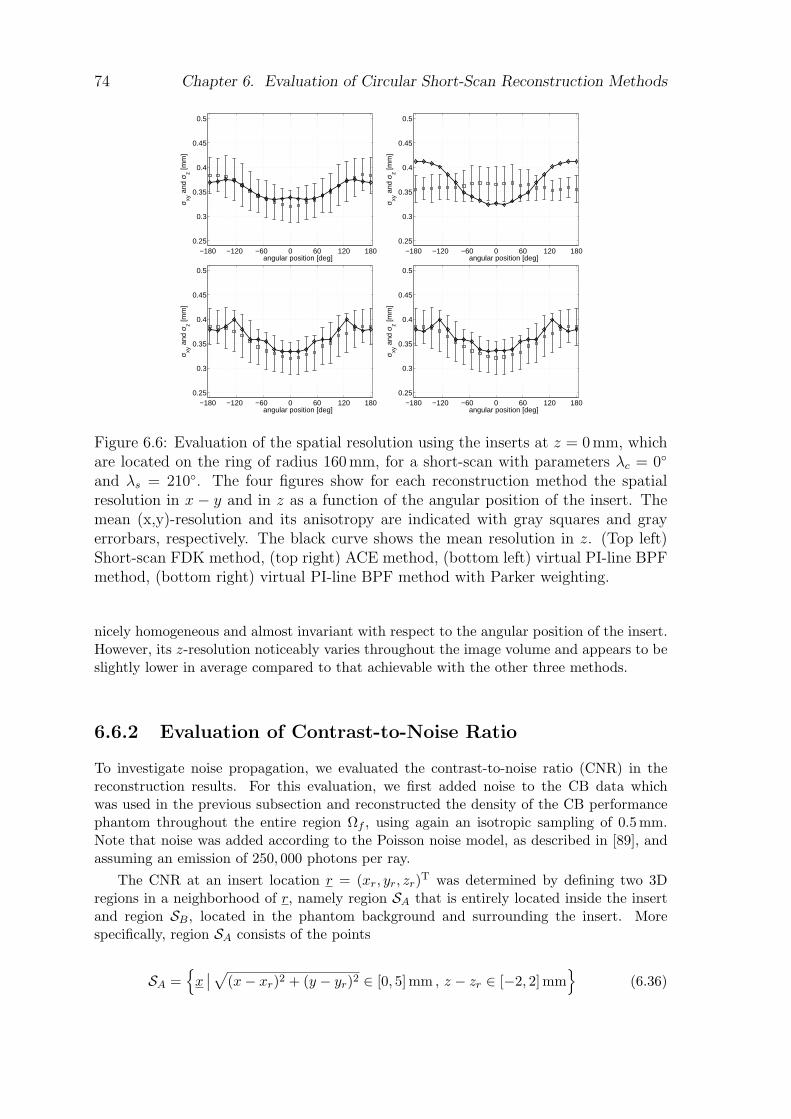
74 Chapter 6. Evaluation of Circular Short-Scan Reconstruction Methods
−180 −120 −60 0 60 120 1800.25
0.3
0.35
0.4
0.45
0.5
angular position [deg]
σ xy a
nd σ
z [mm
]
−180 −120 −60 0 60 120 1800.25
0.3
0.35
0.4
0.45
0.5
angular position [deg]
σ xy a
nd σ
z [mm
]
−180 −120 −60 0 60 120 1800.25
0.3
0.35
0.4
0.45
0.5
angular position [deg]
σ xy a
nd σ
z [mm
]
−180 −120 −60 0 60 120 1800.25
0.3
0.35
0.4
0.45
0.5
angular position [deg]
σ xy a
nd σ
z [mm
]
Figure 6.6: Evaluation of the spatial resolution using the inserts at z = 0 mm, whichare located on the ring of radius 160mm, for a short-scan with parameters λc = 0
and λs = 210. The four figures show for each reconstruction method the spatialresolution in x − y and in z as a function of the angular position of the insert. Themean (x,y)-resolution and its anisotropy are indicated with gray squares and grayerrorbars, respectively. The black curve shows the mean resolution in z. (Top left)Short-scan FDK method, (top right) ACE method, (bottom left) virtual PI-line BPFmethod, (bottom right) virtual PI-line BPF method with Parker weighting.
nicely homogeneous and almost invariant with respect to the angular position of the insert.However, its z-resolution noticeably varies throughout the image volume and appears to beslightly lower in average compared to that achievable with the other three methods.
6.6.2 Evaluation of Contrast-to-Noise Ratio
To investigate noise propagation, we evaluated the contrast-to-noise ratio (CNR) in thereconstruction results. For this evaluation, we first added noise to the CB data whichwas used in the previous subsection and reconstructed the density of the CB performancephantom throughout the entire region Ωf , using again an isotropic sampling of 0.5mm.Note that noise was added according to the Poisson noise model, as described in [89], andassuming an emission of 250, 000 photons per ray.
The CNR at an insert location r = (xr, yr, zr)T was determined by defining two 3Dregions in a neighborhood of r, namely region SA that is entirely located inside the insertand region SB, located in the phantom background and surrounding the insert. Morespecifically, region SA consists of the points
SA =
x∣∣ √
(x− xr)2 + (y − yr)2 ∈ [0, 5]mm , z − zr ∈ [−2, 2]mm
(6.36)
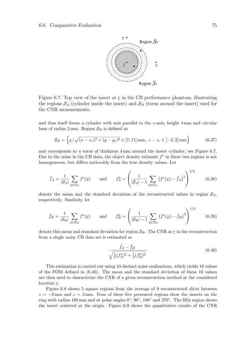
6.6. Comparative Evaluation 75
Figure 6.7: Top view of the insert at r in the CB performance phantom, illustratingthe regions SA (cylinder inside the insert) and SB (torus around the insert) used forthe CNR measurements.
and thus itself forms a cylinder with axis parallel to the z-axis, height 4 mm and circularbase of radius 5 mm. Region SB is defined as
SB =
x |√
(x− xr)2 + (y − yr)2 ∈ [7, 11]mm , z − zr ∈ [−2, 2]mm
(6.37)
and corresponds to a torus of thickness 4 mm around the insert cylinder; see Figure 6.7.Due to the noise in the CB data, the object density estimate fe in these two regions is nothomogeneous, but differs noticeably from the true density values. Let
fA =1|SA|
∑
x∈SA
fe(x) and fσA =
1|SA| − 1
∑
x∈SA
(fe(x)− fA
)2
1/2
(6.38)
denote the mean and the standard deviation of the reconstructed values in region SA,respectively. Similarly, let
fB =1|SB|
∑
x∈SB
fe(x) and fσB =
1|SB| − 1
∑
x∈SB
(fe(x)− fB
)2
1/2
(6.39)
denote this mean and standard deviation for region SB. The CNR at r in the reconstructionfrom a single noisy CB data set is estimated as
fA − fB√12(fσ
A)2 + 12(fσ
B)2. (6.40)
This estimation is carried out using 10 distinct noise realizations, which yields 10 valuesof the FOM defined in (6.40). The mean and the standard deviation of these 10 valuesare then used to characterize the CNR of a given reconstruction method at the consideredlocation r.
Figure 6.8 shows 5 square regions from the average of 9 reconstructed slices betweenz = −2mm and z = 2 mm. Four of these five presented regions show the inserts on thering with radius 160 mm and at polar angles 0, 90, 180 and 270. The fifth region showsthe insert centered at the origin. Figure 6.9 shows the quantitative results of the CNR
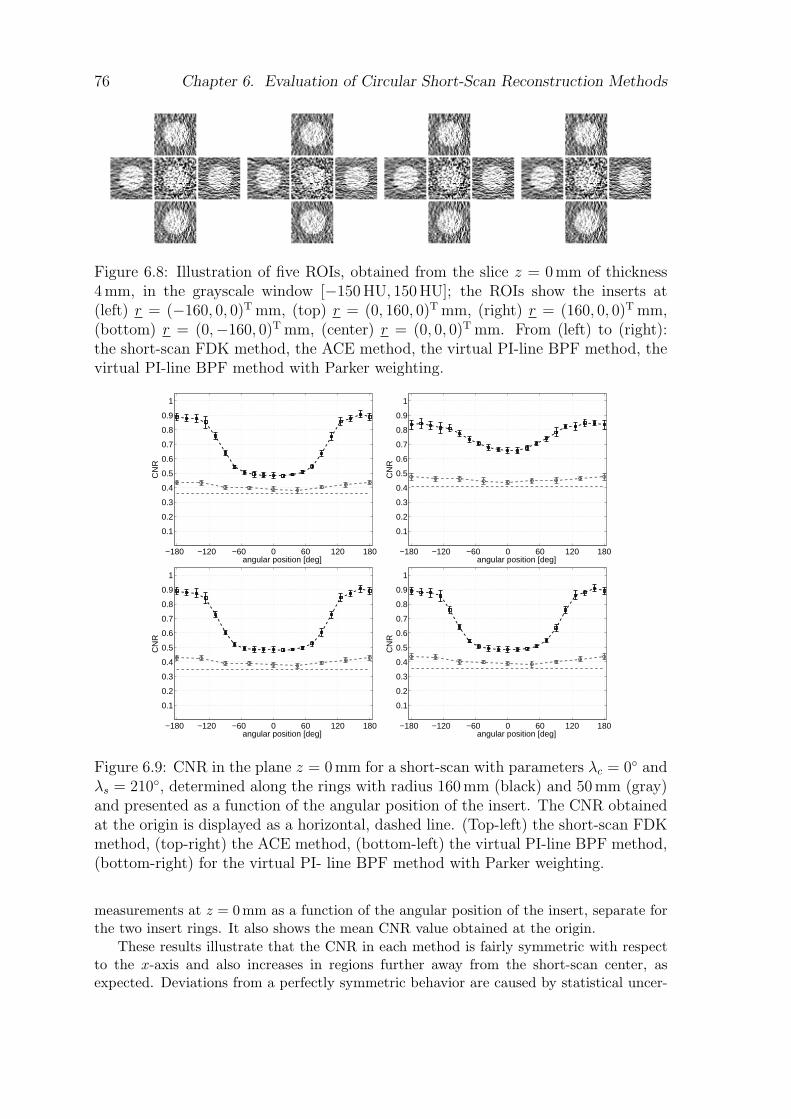
76 Chapter 6. Evaluation of Circular Short-Scan Reconstruction Methods
Figure 6.8: Illustration of five ROIs, obtained from the slice z = 0mm of thickness4mm, in the grayscale window [−150 HU, 150 HU]; the ROIs show the inserts at(left) r = (−160, 0, 0)T mm, (top) r = (0, 160, 0)T mm, (right) r = (160, 0, 0)T mm,(bottom) r = (0,−160, 0)T mm, (center) r = (0, 0, 0)T mm. From (left) to (right):the short-scan FDK method, the ACE method, the virtual PI-line BPF method, thevirtual PI-line BPF method with Parker weighting.
−180 −120 −60 0 60 120 180
0.1
0.2
0.3
0.4
0.5
0.6
0.7
0.8
0.9
1
angular position [deg]
CN
R
−180 −120 −60 0 60 120 180
0.1
0.2
0.3
0.4
0.5
0.6
0.7
0.8
0.9
1
angular position [deg]
CN
R
−180 −120 −60 0 60 120 180
0.1
0.2
0.3
0.4
0.5
0.6
0.7
0.8
0.9
1
angular position [deg]
CN
R
−180 −120 −60 0 60 120 180
0.1
0.2
0.3
0.4
0.5
0.6
0.7
0.8
0.9
1
angular position [deg]
CN
R
Figure 6.9: CNR in the plane z = 0mm for a short-scan with parameters λc = 0 andλs = 210, determined along the rings with radius 160 mm (black) and 50mm (gray)and presented as a function of the angular position of the insert. The CNR obtainedat the origin is displayed as a horizontal, dashed line. (Top-left) the short-scan FDKmethod, (top-right) the ACE method, (bottom-left) the virtual PI-line BPF method,(bottom-right) for the virtual PI- line BPF method with Parker weighting.
measurements at z = 0 mm as a function of the angular position of the insert, separate forthe two insert rings. It also shows the mean CNR value obtained at the origin.
These results illustrate that the CNR in each method is fairly symmetric with respectto the x-axis and also increases in regions further away from the short-scan center, asexpected. Deviations from a perfectly symmetric behavior are caused by statistical uncer-
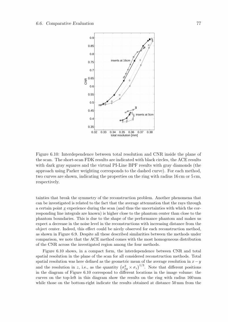
6.6. Comparative Evaluation 77
0.32 0.33 0.34 0.35 0.36 0.37 0.38
0.35
0.4
0.45
0.5
0.55
0.6
0.65
0.7
0.75
0.8
0.85
0.9
total resolution [mm]
CN
R
inserts at 16cm
inserts at 5cm
Figure 6.10: Interdependence between total resolution and CNR inside the plane ofthe scan. The short-scan FDK results are indicated with black circles, the ACE resultswith dark gray squares and the virtual PI-Line BPF results with gray diamonds (theapproach using Parker weighting corresponds to the dashed curve). For each method,two curves are shown, indicating the properties on the ring with radius 16 cm or 5 cm,respectively.
tainties that break the symmetry of the reconstruction problem. Another phenomena thatcan be investigated is related to the fact that the average attenuation that the rays througha certain point x experience during the scan (and thus the uncertainties with which the cor-responding line integrals are known) is higher close to the phantom center than close to thephantom boundaries. This is due to the shape of the performance phantom and makes usexpect a decrease in the noise level in the reconstructions with increasing distance from theobject center. Indeed, this effect could be nicely observed for each reconstruction method,as shown in Figure 6.9. Despite all these described similarities between the methods undercomparison, we note that the ACE method comes with the most homogeneous distributionof the CNR across the investigated region among the four methods.
Figure 6.10 shows, in a compact form, the interdependence between CNR and totalspatial resolution in the plane of the scan for all considered reconstruction methods. Totalspatial resolution was here defined as the geometric mean of the average resolution in x− y
and the resolution in z, i.e., as the quantity(σ2
xy × σz
)1/3. Note that different positionsin the diagram of Figure 6.10 correspond to different locations in the image volume: thecurves on the top-left in this diagram show the results on the ring with radius 160 mmwhile those on the bottom-right indicate the results obtained at distance 50 mm from the
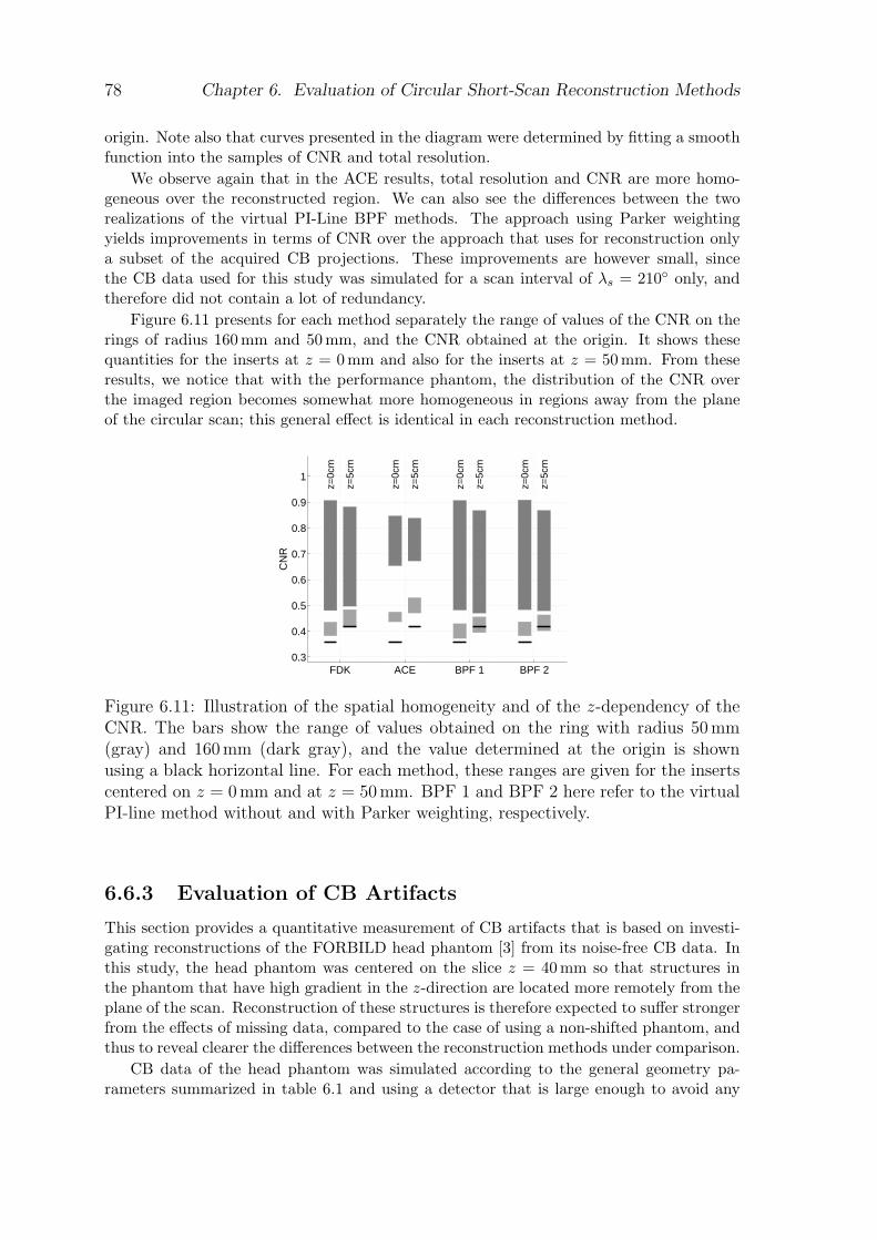
78 Chapter 6. Evaluation of Circular Short-Scan Reconstruction Methods
origin. Note also that curves presented in the diagram were determined by fitting a smoothfunction into the samples of CNR and total resolution.
We observe again that in the ACE results, total resolution and CNR are more homo-geneous over the reconstructed region. We can also see the differences between the tworealizations of the virtual PI-Line BPF methods. The approach using Parker weightingyields improvements in terms of CNR over the approach that uses for reconstruction onlya subset of the acquired CB projections. These improvements are however small, sincethe CB data used for this study was simulated for a scan interval of λs = 210 only, andtherefore did not contain a lot of redundancy.
Figure 6.11 presents for each method separately the range of values of the CNR on therings of radius 160 mm and 50 mm, and the CNR obtained at the origin. It shows thesequantities for the inserts at z = 0mm and also for the inserts at z = 50 mm. From theseresults, we notice that with the performance phantom, the distribution of the CNR overthe imaged region becomes somewhat more homogeneous in regions away from the planeof the circular scan; this general effect is identical in each reconstruction method.
FDK ACE BPF 1 BPF 20.3
0.4
0.5
0.6
0.7
0.8
0.9
1
z=0c
m
z=5c
m
z=0c
m
z=5c
m
z=0c
m
z=5c
m
z=0c
m
z=5c
m
CN
R
Figure 6.11: Illustration of the spatial homogeneity and of the z-dependency of theCNR. The bars show the range of values obtained on the ring with radius 50mm(gray) and 160 mm (dark gray), and the value determined at the origin is shownusing a black horizontal line. For each method, these ranges are given for the insertscentered on z = 0mm and at z = 50mm. BPF 1 and BPF 2 here refer to the virtualPI-line method without and with Parker weighting, respectively.
6.6.3 Evaluation of CB Artifacts
This section provides a quantitative measurement of CB artifacts that is based on investi-gating reconstructions of the FORBILD head phantom [3] from its noise-free CB data. Inthis study, the head phantom was centered on the slice z = 40 mm so that structures inthe phantom that have high gradient in the z-direction are located more remotely from theplane of the scan. Reconstruction of these structures is therefore expected to suffer strongerfrom the effects of missing data, compared to the case of using a non-shifted phantom, andthus to reveal clearer the differences between the reconstruction methods under comparison.
CB data of the head phantom was simulated according to the general geometry pa-rameters summarized in table 6.1 and using a detector that is large enough to avoid any
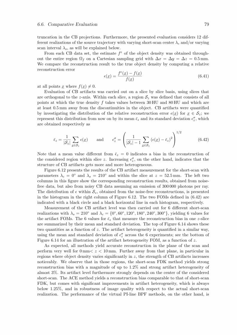
6.6. Comparative Evaluation 79
truncation in the CB projections. Furthermore, the presented evaluation considers 12 dif-ferent realizations of the source trajectory with varying short-scan center λc and/or varyingscan interval λs, as will be explained below.
From each CB data set, the estimate fe of the object density was obtained through-out the entire region Ωf on a Cartesian sampling grid with ∆x = ∆y = ∆z = 0.5mm.We compare the reconstruction result to the true object density by computing a relativereconstruction error
ε(x) =fe(x)− f(x)
f(x)(6.41)
at all points x where f(x) 6= 0.Evaluation of CB artifacts was carried out on a slice by slice basis, using slices that
are orthogonal to the z-axis. Within each slice, a region Sz was defined that consists of allpoints at which the true density f takes values between 30 HU and 80 HU and which areat least 0.5mm away from the discontinuities in the object. CB artifacts were quantifiedby investigating the distribution of the relative reconstruction error ε(x) for x ∈ Sz; werepresent this distribution from now on by its mean εz and its standard deviation εσ
z , whichare obtained respectively as
εz =1|Sz|
∑
x∈Sz
ε(x) and εσz =
1|Sz| − 1
∑
x∈Sz
(ε(x)− εz)2
1/2
(6.42)
Note that a mean value different from εz = 0 indicates a bias in the reconstruction ofthe considered region within slice z. Increasing εσ
z , on the other hand, indicates that thestructure of CB artifacts gets more and more heterogeneous.
Figure 6.12 presents the results of the CB artifact measurement for the short-scan withparameters λc = 0 and λs = 210 and within the slice at z = 52.5mm. The left twocolumns in this figure show the corresponding reconstruction results, obtained from noise-free data, but also from noisy CB data assuming an emission of 300 000 photons per ray.The distribution of ε within Sz, obtained from the noise-free reconstructions, is presentedin the histogram in the right column of Figure 6.12. The two FOMs defined in (6.42) areindicated with a black circle and a black horizontal line in each histogram, respectively.
Measurement of the CB artifact level was then carried out for 6 different short-scanrealizations with λs = 210 and λc = 0, 60, 120, 180, 240, 300, yielding 6 values forthe artifact FOMs. The 6 values for εz that measure the reconstruction bias in one z-sliceare summarized by their mean and standard deviation. The top of Figure 6.14 shows thesetwo quantities as a function of z. The artifact heterogeneity is quantified in a similar way,using the mean and standard deviation of εσ
z across the 6 experiments; see the bottom ofFigure 6.14 for an illustration of the artifact heterogeneity FOM, as a function of z.
As expected, all methods yield accurate reconstruction in the plane of the scan andperform very well for 0 mm< z < 10mm. Further away from that plane, in particular inregions where object density varies significantly in z, the strength of CB artifacts increasesnoticeably. We observe that in those regions, the short-scan FDK method yields strongreconstruction bias with a magnitude of up to 1.2% and strong artifact heterogeneity ofalmost 3%. Its artifact level furthermore strongly depends on the center of the consideredshort-scan. The ACE method yields a reconstruction bias comparable to that of short-scanFDK, but comes with significant improvements in artifact heterogeneity, which is alwaysbelow 1.25%, and in robustness of image quality with respect to the actual short-scanrealization. The performance of the virtual PI-line BPF methods, on the other hand, is
80 Chapter 6. Evaluation of Circular Short-Scan Reconstruction Methods
−2 −1 0 1 20
5
10
15
20
relative error [%]
area
[cm
2 ]
−2 −1 0 1 20
5
10
15
20
relative error [%]
area
[cm
2 ]
−2 −1 0 1 20
5
10
15
20
relative error [%]
area
[cm
2 ]
−2 −1 0 1 20
5
10
15
20
relative error [%]
area
[cm
2 ]
Figure 6.12: The slice z = 52.5mm through the reconstructions of the FORBILDhead phantom using a short-scan defined with λc = 0, λs = 210 and obtained usingfrom (top) to (bottom): the short-scan FDK method, the ACE method, the virtualPI-line BPF method and the virtual PI-line BPF method with Parker weighting.(Left) reconstructions from noisy data assuming 300 000 photons per ray in the gray-scale window [0 HU, 100 HU], (center row) reconstructions from noise-free CB datain the gray-scale window [0 HU, 100 HU] and (right) histograms of the relative recon-struction error for the values in the region Sz. The horizontal bar in each histogramshows the first moment (circle) and second moment (half-width of the bar) of thehistogram.
superior to that of the other evaluated methods considering reconstruction bias (whichis less than 0.75%), but shows like short-scan FDK disadvantages in terms of artifact
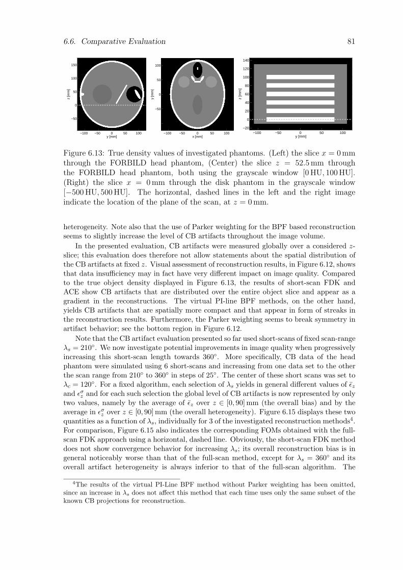
6.6. Comparative Evaluation 81
y [mm]
z [m
m]
−100 −50 0 50 100
−50
0
50
100
150
x [mm]
y [m
m]
−100 −50 0 50 100
−50
0
50
100
y [mm]
z [m
m]
−100 −50 0 50 100−20
0
20
40
60
80
100
120
140
Figure 6.13: True density values of investigated phantoms. (Left) the slice x = 0mmthrough the FORBILD head phantom, (Center) the slice z = 52.5mm throughthe FORBILD head phantom, both using the grayscale window [0 HU, 100 HU].(Right) the slice x = 0 mm through the disk phantom in the grayscale window[−500 HU, 500 HU]. The horizontal, dashed lines in the left and the right imageindicate the location of the plane of the scan, at z = 0mm.
heterogeneity. Note also that the use of Parker weighting for the BPF based reconstructionseems to slightly increase the level of CB artifacts throughout the image volume.
In the presented evaluation, CB artifacts were measured globally over a considered z-slice; this evaluation does therefore not allow statements about the spatial distribution ofthe CB artifacts at fixed z. Visual assessment of reconstruction results, in Figure 6.12, showsthat data insufficiency may in fact have very different impact on image quality. Comparedto the true object density displayed in Figure 6.13, the results of short-scan FDK andACE show CB artifacts that are distributed over the entire object slice and appear as agradient in the reconstructions. The virtual PI-line BPF methods, on the other hand,yields CB artifacts that are spatially more compact and that appear in form of streaks inthe reconstruction results. Furthermore, the Parker weighting seems to break symmetry inartifact behavior; see the bottom region in Figure 6.12.
Note that the CB artifact evaluation presented so far used short-scans of fixed scan-rangeλs = 210. We now investigate potential improvements in image quality when progressivelyincreasing this short-scan length towards 360. More specifically, CB data of the headphantom were simulated using 6 short-scans and increasing from one data set to the otherthe scan range from 210 to 360 in steps of 25. The center of these short scans was set toλc = 120. For a fixed algorithm, each selection of λs yields in general different values of εz
and εσz and for each such selection the global level of CB artifacts is now represented by only
two values, namely by the average of εz over z ∈ [0, 90] mm (the overall bias) and by theaverage in εσ
z over z ∈ [0, 90]mm (the overall heterogeneity). Figure 6.15 displays these twoquantities as a function of λs, individually for 3 of the investigated reconstruction methods4.For comparison, Figure 6.15 also indicates the corresponding FOMs obtained with the full-scan FDK approach using a horizontal, dashed line. Obviously, the short-scan FDK methoddoes not show convergence behavior for increasing λs; its overall reconstruction bias is ingeneral noticeably worse than that of the full-scan method, except for λs = 360 and itsoverall artifact heterogeneity is always inferior to that of the full-scan algorithm. The
4The results of the virtual PI-Line BPF method without Parker weighting has been omitted,since an increase in λs does not affect this method that each time uses only the same subset of theknown CB projections for reconstruction.
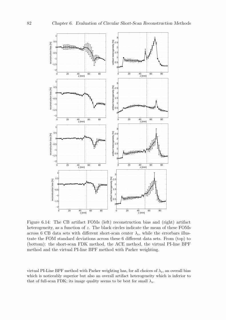
82 Chapter 6. Evaluation of Circular Short-Scan Reconstruction Methods
0 20 40 60 80
−2
−1.5
−1
−0.5
0
0.5
1
z [mm]
reco
nstr
uctio
n bi
as [%
]
0 20 40 60 80
0
0.5
1
1.5
2
2.5
3
z [mm]
artif
act h
eter
ogen
eity
[%]
0 20 40 60 80
−2
−1.5
−1
−0.5
0
0.5
1
z [mm]
reco
nstr
uctio
n bi
as [%
]
0 20 40 60 80
0
0.5
1
1.5
2
2.5
3
z [mm]
artif
act h
eter
ogen
eity
[%]
0 20 40 60 80
−2
−1.5
−1
−0.5
0
0.5
1
z [mm]
reco
nstr
uctio
n bi
as [%
]
0 20 40 60 80
0
0.5
1
1.5
2
2.5
3
z [mm]
artif
act h
eter
ogen
eity
[%]
0 20 40 60 80
−2
−1.5
−1
−0.5
0
0.5
1
z [mm]
reco
nstr
uctio
n bi
as [%
]
0 20 40 60 80
0
0.5
1
1.5
2
2.5
3
z [mm]
artif
act h
eter
ogen
eity
[%]
Figure 6.14: The CB artifact FOMs (left) reconstruction bias and (right) artifactheterogeneity, as a function of z. The black circles indicate the mean of these FOMsacross 6 CB data sets with different short-scan center λc, while the errorbars illus-trate the FOM standard deviations across these 6 different data sets. From (top) to(bottom): the short-scan FDK method, the ACE method, the virtual PI-line BPFmethod and the virtual PI-line BPF method with Parker weighting.
virtual PI-Line BPF method with Parker weighting has, for all choices of λs, an overall biaswhich is noticeably superior but also an overall artifact heterogeneity which is inferior tothat of full-scan FDK; its image quality seems to be best for small λs.
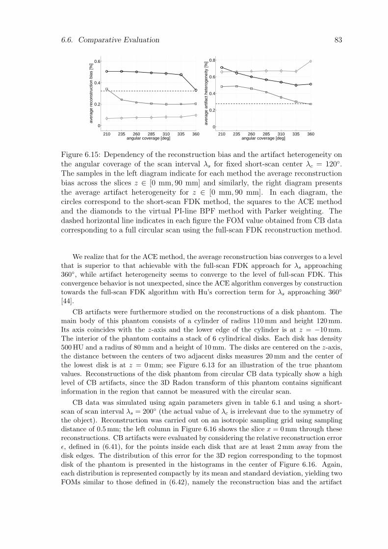
6.6. Comparative Evaluation 83
210 235 260 285 310 335 360
0
0.2
0.4
0.6
angular coverage [deg]
aver
age
reco
nstr
uctio
n bi
as [%
]
210 235 260 285 310 335 360
0
0.2
0.4
0.6
0.8
angular coverage [deg]
aver
age
artif
act h
eter
ogen
eity
[%]
Figure 6.15: Dependency of the reconstruction bias and the artifact heterogeneity onthe angular coverage of the scan interval λs for fixed short-scan center λc = 120.The samples in the left diagram indicate for each method the average reconstructionbias across the slices z ∈ [0 mm, 90 mm] and similarly, the right diagram presentsthe average artifact heterogeneity for z ∈ [0 mm, 90 mm]. In each diagram, thecircles correspond to the short-scan FDK method, the squares to the ACE methodand the diamonds to the virtual PI-line BPF method with Parker weighting. Thedashed horizontal line indicates in each figure the FOM value obtained from CB datacorresponding to a full circular scan using the full-scan FDK reconstruction method.
We realize that for the ACE method, the average reconstruction bias converges to a levelthat is superior to that achievable with the full-scan FDK approach for λs approaching360, while artifact heterogeneity seems to converge to the level of full-scan FDK. Thisconvergence behavior is not unexpected, since the ACE algorithm converges by constructiontowards the full-scan FDK algorithm with Hu’s correction term for λs approaching 360
[44].
CB artifacts were furthermore studied on the reconstructions of a disk phantom. Themain body of this phantom consists of a cylinder of radius 110mm and height 120 mm.Its axis coincides with the z-axis and the lower edge of the cylinder is at z = −10 mm.The interior of the phantom contains a stack of 6 cylindrical disks. Each disk has density500HU and a radius of 80 mm and a height of 10 mm. The disks are centered on the z-axis,the distance between the centers of two adjacent disks measures 20 mm and the center ofthe lowest disk is at z = 0mm; see Figure 6.13 for an illustration of the true phantomvalues. Reconstructions of the disk phantom from circular CB data typically show a highlevel of CB artifacts, since the 3D Radon transform of this phantom contains significantinformation in the region that cannot be measured with the circular scan.
CB data was simulated using again parameters given in table 6.1 and using a short-scan of scan interval λs = 200 (the actual value of λc is irrelevant due to the symmetry ofthe object). Reconstruction was carried out on an isotropic sampling grid using samplingdistance of 0.5mm; the left column in Figure 6.16 shows the slice x = 0 mm through thesereconstructions. CB artifacts were evaluated by considering the relative reconstruction errorε, defined in (6.41), for the points inside each disk that are at least 2mm away from thedisk edges. The distribution of this error for the 3D region corresponding to the topmostdisk of the phantom is presented in the histograms in the center of Figure 6.16. Again,each distribution is represented compactly by its mean and standard deviation, yielding twoFOMs similar to those defined in (6.42), namely the reconstruction bias and the artifact
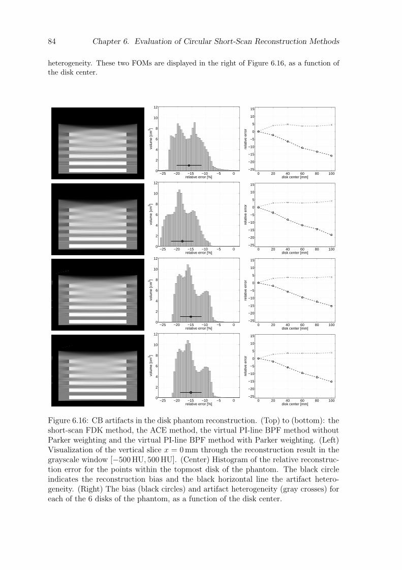
84 Chapter 6. Evaluation of Circular Short-Scan Reconstruction Methods
heterogeneity. These two FOMs are displayed in the right of Figure 6.16, as a function ofthe disk center.
−25 −20 −15 −10 −5 00
2
4
6
8
10
12
relative error [%]
volu
me
[cm
3 ]
0 20 40 60 80 100−25
−20
−15
−10
−5
0
5
10
15
disk center [mm]
rela
tive
erro
r−25 −20 −15 −10 −5 0
0
2
4
6
8
10
12
relative error [%]
volu
me
[cm
3 ]
0 20 40 60 80 100−25
−20
−15
−10
−5
0
5
10
15
disk center [mm]
rela
tive
erro
r
−25 −20 −15 −10 −5 00
2
4
6
8
10
12
relative error [%]
volu
me
[cm
3 ]
0 20 40 60 80 100−25
−20
−15
−10
−5
0
5
10
15
disk center [mm]
rela
tive
erro
r
−25 −20 −15 −10 −5 00
2
4
6
8
10
12
relative error [%]
volu
me
[cm
3 ]
0 20 40 60 80 100−25
−20
−15
−10
−5
0
5
10
15
disk center [mm]
rela
tive
erro
r
Figure 6.16: CB artifacts in the disk phantom reconstruction. (Top) to (bottom): theshort-scan FDK method, the ACE method, the virtual PI-line BPF method withoutParker weighting and the virtual PI-line BPF method with Parker weighting. (Left)Visualization of the vertical slice x = 0mm through the reconstruction result in thegrayscale window [−500 HU, 500 HU]. (Center) Histogram of the relative reconstruc-tion error for the points within the topmost disk of the phantom. The black circleindicates the reconstruction bias and the black horizontal line the artifact hetero-geneity. (Right) The bias (black circles) and artifact heterogeneity (gray crosses) foreach of the 6 disks of the phantom, as a function of the disk center.
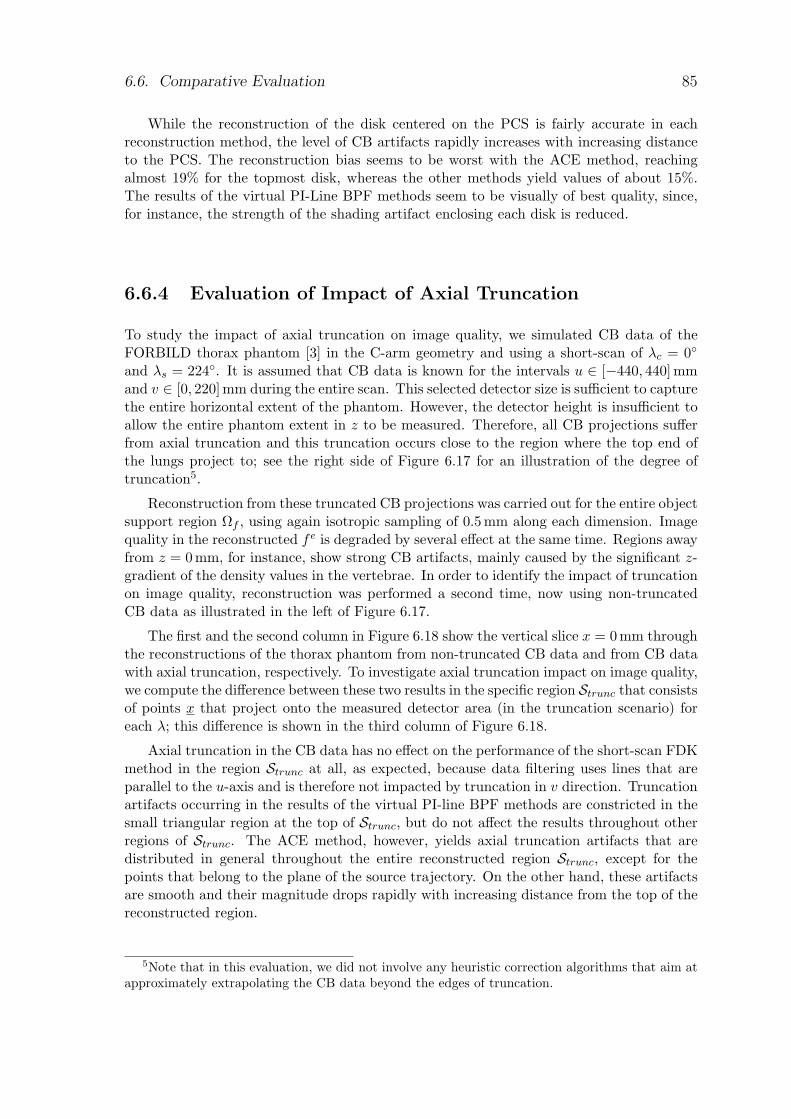
6.6. Comparative Evaluation 85
While the reconstruction of the disk centered on the PCS is fairly accurate in eachreconstruction method, the level of CB artifacts rapidly increases with increasing distanceto the PCS. The reconstruction bias seems to be worst with the ACE method, reachingalmost 19% for the topmost disk, whereas the other methods yield values of about 15%.The results of the virtual PI-Line BPF methods seem to be visually of best quality, since,for instance, the strength of the shading artifact enclosing each disk is reduced.
6.6.4 Evaluation of Impact of Axial Truncation
To study the impact of axial truncation on image quality, we simulated CB data of theFORBILD thorax phantom [3] in the C-arm geometry and using a short-scan of λc = 0
and λs = 224. It is assumed that CB data is known for the intervals u ∈ [−440, 440]mmand v ∈ [0, 220]mm during the entire scan. This selected detector size is sufficient to capturethe entire horizontal extent of the phantom. However, the detector height is insufficient toallow the entire phantom extent in z to be measured. Therefore, all CB projections sufferfrom axial truncation and this truncation occurs close to the region where the top end ofthe lungs project to; see the right side of Figure 6.17 for an illustration of the degree oftruncation5.
Reconstruction from these truncated CB projections was carried out for the entire objectsupport region Ωf , using again isotropic sampling of 0.5mm along each dimension. Imagequality in the reconstructed fe is degraded by several effect at the same time. Regions awayfrom z = 0mm, for instance, show strong CB artifacts, mainly caused by the significant z-gradient of the density values in the vertebrae. In order to identify the impact of truncationon image quality, reconstruction was performed a second time, now using non-truncatedCB data as illustrated in the left of Figure 6.17.
The first and the second column in Figure 6.18 show the vertical slice x = 0 mm throughthe reconstructions of the thorax phantom from non-truncated CB data and from CB datawith axial truncation, respectively. To investigate axial truncation impact on image quality,we compute the difference between these two results in the specific region Strunc that consistsof points x that project onto the measured detector area (in the truncation scenario) foreach λ; this difference is shown in the third column of Figure 6.18.
Axial truncation in the CB data has no effect on the performance of the short-scan FDKmethod in the region Strunc at all, as expected, because data filtering uses lines that areparallel to the u-axis and is therefore not impacted by truncation in v direction. Truncationartifacts occurring in the results of the virtual PI-line BPF methods are constricted in thesmall triangular region at the top of Strunc, but do not affect the results throughout otherregions of Strunc. The ACE method, however, yields axial truncation artifacts that aredistributed in general throughout the entire reconstructed region Strunc, except for thepoints that belong to the plane of the source trajectory. On the other hand, these artifactsare smooth and their magnitude drops rapidly with increasing distance from the top of thereconstructed region.
5Note that in this evaluation, we did not involve any heuristic correction algorithms that aim atapproximately extrapolating the CB data beyond the edges of truncation.
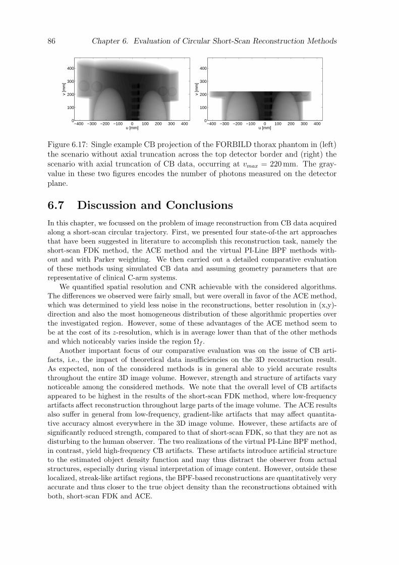
86 Chapter 6. Evaluation of Circular Short-Scan Reconstruction Methods
u [mm]
v [m
m]
−400 −300 −200 −100 0 100 200 300 4000
100
200
300
400
u [mm]
v [m
m]
−400 −300 −200 −100 0 100 200 300 4000
100
200
300
400
Figure 6.17: Single example CB projection of the FORBILD thorax phantom in (left)the scenario without axial truncation across the top detector border and (right) thescenario with axial truncation of CB data, occurring at vmax = 220mm. The gray-value in these two figures encodes the number of photons measured on the detectorplane.
6.7 Discussion and Conclusions
In this chapter, we focussed on the problem of image reconstruction from CB data acquiredalong a short-scan circular trajectory. First, we presented four state-of-the art approachesthat have been suggested in literature to accomplish this reconstruction task, namely theshort-scan FDK method, the ACE method and the virtual PI-Line BPF methods with-out and with Parker weighting. We then carried out a detailed comparative evaluationof these methods using simulated CB data and assuming geometry parameters that arerepresentative of clinical C-arm systems.
We quantified spatial resolution and CNR achievable with the considered algorithms.The differences we observed were fairly small, but were overall in favor of the ACE method,which was determined to yield less noise in the reconstructions, better resolution in (x,y)-direction and also the most homogeneous distribution of these algorithmic properties overthe investigated region. However, some of these advantages of the ACE method seem tobe at the cost of its z-resolution, which is in average lower than that of the other methodsand which noticeably varies inside the region Ωf .
Another important focus of our comparative evaluation was on the issue of CB arti-facts, i.e., the impact of theoretical data insufficiencies on the 3D reconstruction result.As expected, non of the considered methods is in general able to yield accurate resultsthroughout the entire 3D image volume. However, strength and structure of artifacts varynoticeable among the considered methods. We note that the overall level of CB artifactsappeared to be highest in the results of the short-scan FDK method, where low-frequencyartifacts affect reconstruction throughout large parts of the image volume. The ACE resultsalso suffer in general from low-frequency, gradient-like artifacts that may affect quantita-tive accuracy almost everywhere in the 3D image volume. However, these artifacts are ofsignificantly reduced strength, compared to that of short-scan FDK, so that they are not asdisturbing to the human observer. The two realizations of the virtual PI-Line BPF method,in contrast, yield high-frequency CB artifacts. These artifacts introduce artificial structureto the estimated object density function and may thus distract the observer from actualstructures, especially during visual interpretation of image content. However, outside theselocalized, streak-like artifact regions, the BPF-based reconstructions are quantitatively veryaccurate and thus closer to the true object density than the reconstructions obtained withboth, short-scan FDK and ACE.
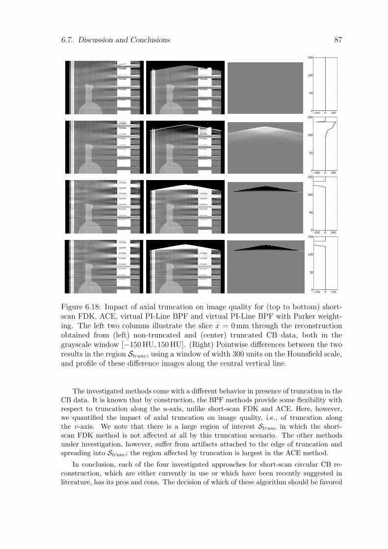
6.7. Discussion and Conclusions 87
−100 0 1000
50
100
150
−100 0 1000
50
100
150
−100 0 1000
50
100
150
−100 0 1000
50
100
150
Figure 6.18: Impact of axial truncation on image quality for (top to bottom) short-scan FDK, ACE, virtual PI-Line BPF and virtual PI-Line BPF with Parker weight-ing. The left two columns illustrate the slice x = 0mm through the reconstructionobtained from (left) non-truncated and (center) truncated CB data, both in thegrayscale window [−150 HU, 150 HU]. (Right) Pointwise differences between the tworesults in the region Strunc, using a window of width 300 units on the Hounsfield scale,and profile of these difference images along the central vertical line.
The investigated methods come with a different behavior in presence of truncation in theCB data. It is known that by construction, the BPF methods provide some flexibility withrespect to truncation along the u-axis, unlike short-scan FDK and ACE. Here, however,we quantified the impact of axial truncation on image quality, i.e., of truncation alongthe v-axis. We note that there is a large region of interest Strunc in which the short-scan FDK method is not affected at all by this truncation scenario. The other methodsunder investigation, however, suffer from artifacts attached to the edge of truncation andspreading into Strunc; the region affected by truncation is largest in the ACE method.
In conclusion, each of the four investigated approaches for short-scan circular CB re-construction, which are either currently in use or which have been recently suggested inliterature, has its pros and cons. The decision of which of these algorithm should be favored

88 Chapter 6. Evaluation of Circular Short-Scan Reconstruction Methods
for practical purposes thus highly depends on the imaging application and also on the classof investigated objects. Short-scan FDK, for instance, is computationally very efficient andcomes with low (axial) detector requirements. The ACE method has advantages in imagenoise and CB artifacts only appear as low-contrast, low-frequency image defects. The BPFmethods, on the other hand, are quantitatively most accurate and can deal with some sce-narios of transaxial truncation, but at the cost of occasional streak artifacts. Finding anefficacious analytical circular short-scan reconstruction algorithm that brings advantages inevery aspect of image quality is a highly complex issue and an overall satisfying solutionmay not exist due to the data incompleteness.
Chapter 7
A Factorization Method forCircular Short-Scan CBReconstruction
7.1 Introduction
In this chapter, we present a novel, original method for CB image reconstruction in theshort scan circular acquisition geometry. Our method is based on a theoretically-exactfactorization of the 3D short-scan CB reconstruction problem into a set of independent 2Dinversion problems, each of which corresponds to finding the object density on one plane.Reconstruction involves an iterative algorithm to numerically solve these 2D inversion prob-lems on a one-by-one basis. Reconstruction of the entire 3D image volume is achieved bycombining the results from each 2D inversion problem. The fundamental property of ourfactorization approach, which distinguishes it from the reconstruction methods comparedin chapter 6, are its ability to perform reconstruction without involving geometric approx-imations and to enforce all reconstructed values to be positive. These properties make thefactorization approach similar to 3D iterative reconstruction approaches; see for instance[35]. The latter, however, achieve reconstruction using 3D iterations, which is computation-ally demanding; our factorization approach, in contrast, involves only a set of 2D iterationsand is thus more efficient.
7.2 Reconstruction Theory
This section presents the theoretical background underlying our reconstruction approach.We describe, in particular, how the factorization of the circular CB reconstruction problemis established and describe its usefulness for reconstruction of a 3D volume of interest.
7.2.1 The Plane of Interest POur method targets reconstruction within planes that are parallel to the z-axis and thatintersect the source trajectory at two locations. Let P be such a plane of interest and letλ1 and λ2 with λmin ≤ λ1 < λ2 ≤ λmax denote the source polar angles where P hits thesource trajectory. By construction, the source positions a(λ1) and a(λ2) both belong to P.
89
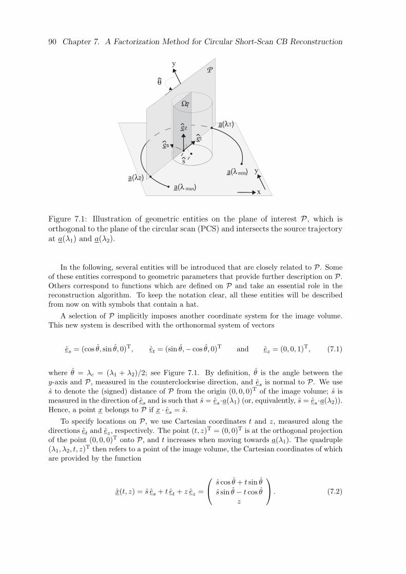
90 Chapter 7. A Factorization Method for Circular Short-Scan CB Reconstruction
s
y
max
amin
y
x
ee
e
a
a
a
Figure 7.1: Illustration of geometric entities on the plane of interest P , which isorthogonal to the plane of the circular scan (PCS) and intersects the source trajectoryat a(λ1) and a(λ2).
In the following, several entities will be introduced that are closely related to P. Someof these entities correspond to geometric parameters that provide further description on P.Others correspond to functions which are defined on P and take an essential role in thereconstruction algorithm. To keep the notation clear, all these entities will be describedfrom now on with symbols that contain a hat.
A selection of P implicitly imposes another coordinate system for the image volume.This new system is described with the orthonormal system of vectors
es = (cos θ, sin θ, 0)T, et = (sin θ,− cos θ, 0)T and ez = (0, 0, 1)T, (7.1)
where θ = λc = (λ1 + λ2)/2; see Figure 7.1. By definition, θ is the angle between they-axis and P, measured in the counterclockwise direction, and es is normal to P. We uses to denote the (signed) distance of P from the origin (0, 0, 0)T of the image volume; s ismeasured in the direction of es and is such that s = es ·a(λ1) (or, equivalently, s = es ·a(λ2)).Hence, a point x belongs to P if x · es = s.
To specify locations on P, we use Cartesian coordinates t and z, measured along thedirections et and ez, respectively. The point (t, z)T = (0, 0)T is at the orthogonal projectionof the point (0, 0, 0)T onto P, and t increases when moving towards a(λ1). The quadruple(λ1, λ2, t, z)T then refers to a point of the image volume, the Cartesian coordinates of whichare provided by the function
x(t, z) = s es + t et + z ez =
s cos θ + t sin θ
s sin θ − t cos θz
. (7.2)
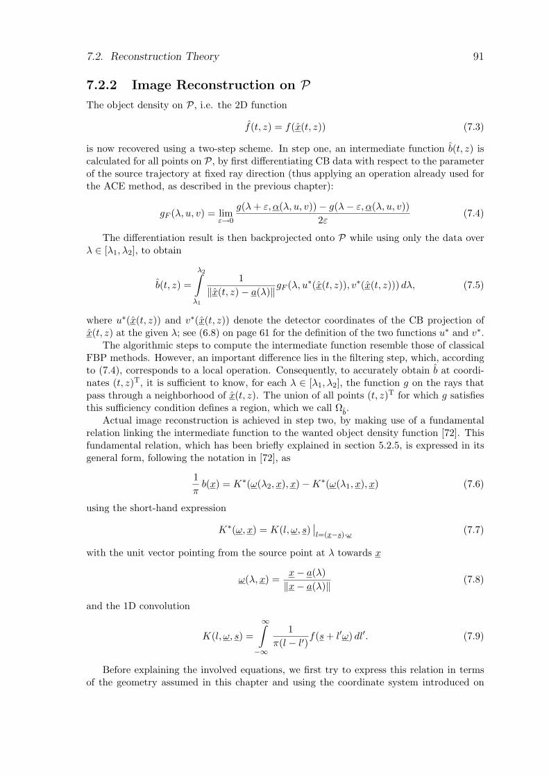
7.2. Reconstruction Theory 91
7.2.2 Image Reconstruction on PThe object density on P, i.e. the 2D function
f(t, z) = f(x(t, z)) (7.3)
is now recovered using a two-step scheme. In step one, an intermediate function b(t, z) iscalculated for all points on P, by first differentiating CB data with respect to the parameterof the source trajectory at fixed ray direction (thus applying an operation already used forthe ACE method, as described in the previous chapter):
gF (λ, u, v) = limε→0
g(λ + ε, α(λ, u, v))− g(λ− ε, α(λ, u, v))2ε
(7.4)
The differentiation result is then backprojected onto P while using only the data overλ ∈ [λ1, λ2], to obtain
b(t, z) =
λ2∫
λ1
1‖x(t, z)− a(λ)‖gF (λ, u∗(x(t, z)), v∗(x(t, z))) dλ, (7.5)
where u∗(x(t, z)) and v∗(x(t, z)) denote the detector coordinates of the CB projection ofx(t, z) at the given λ; see (6.8) on page 61 for the definition of the two functions u∗ and v∗.
The algorithmic steps to compute the intermediate function resemble those of classicalFBP methods. However, an important difference lies in the filtering step, which, accordingto (7.4), corresponds to a local operation. Consequently, to accurately obtain b at coordi-nates (t, z)T, it is sufficient to know, for each λ ∈ [λ1, λ2], the function g on the rays thatpass through a neighborhood of x(t, z). The union of all points (t, z)T for which g satisfiesthis sufficiency condition defines a region, which we call Ωb.
Actual image reconstruction is achieved in step two, by making use of a fundamentalrelation linking the intermediate function to the wanted object density function [72]. Thisfundamental relation, which has been briefly explained in section 5.2.5, is expressed in itsgeneral form, following the notation in [72], as
1π
b(x) = K∗(ω(λ2, x), x)−K∗(ω(λ1, x), x) (7.6)
using the short-hand expression
K∗(ω, x) = K(l, ω, s)∣∣l=(x−s)·ω (7.7)
with the unit vector pointing from the source point at λ towards x
ω(λ, x) =x− a(λ)‖x− a(λ)‖ (7.8)
and the 1D convolution
K(l, ω, s) =
∞∫
−∞
1π(l − l′)
f(s + l′ω) dl′. (7.9)
Before explaining the involved equations, we first try to express this relation in termsof the geometry assumed in this chapter and using the coordinate system introduced on
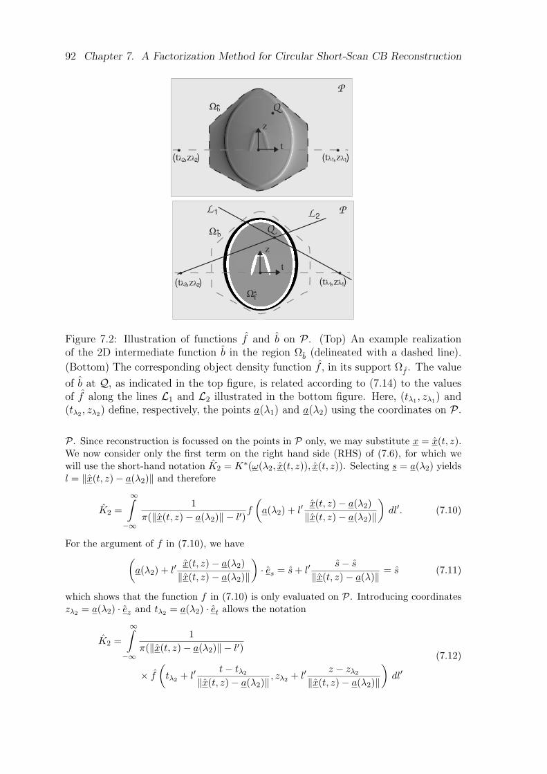
92 Chapter 7. A Factorization Method for Circular Short-Scan CB Reconstruction
b
t
t tz z
z
b
f
t
t tz z
z
Figure 7.2: Illustration of functions f and b on P . (Top) An example realizationof the 2D intermediate function b in the region Ωb (delineated with a dashed line).
(Bottom) The corresponding object density function f , in its support Ωf . The value
of b at Q, as indicated in the top figure, is related according to (7.14) to the valuesof f along the lines L1 and L2 illustrated in the bottom figure. Here, (tλ1 , zλ1) and(tλ2 , zλ2) define, respectively, the points a(λ1) and a(λ2) using the coordinates on P .
P. Since reconstruction is focussed on the points in P only, we may substitute x = x(t, z).We now consider only the first term on the right hand side (RHS) of (7.6), for which wewill use the short-hand notation K2 = K∗(ω(λ2, x(t, z)), x(t, z)). Selecting s = a(λ2) yieldsl = ‖x(t, z)− a(λ2)‖ and therefore
K2 =
∞∫
−∞
1π(‖x(t, z)− a(λ2)‖ − l′)
f
(a(λ2) + l′
x(t, z)− a(λ2)‖x(t, z)− a(λ2)‖
)dl′. (7.10)
For the argument of f in (7.10), we have(
a(λ2) + l′x(t, z)− a(λ2)‖x(t, z)− a(λ2)‖
)· es = s + l′
s− s
‖x(t, z)− a(λ)‖ = s (7.11)
which shows that the function f in (7.10) is only evaluated on P. Introducing coordinateszλ2 = a(λ2) · ez and tλ2 = a(λ2) · et allows the notation
K2 =
∞∫
−∞
1π(‖x(t, z)− a(λ2)‖ − l′)
× f
(tλ2 + l′
t− tλ2
‖x(t, z)− a(λ2)‖ , zλ2 + l′z − zλ2
‖x(t, z)− a(λ2)‖)
dl′
(7.12)
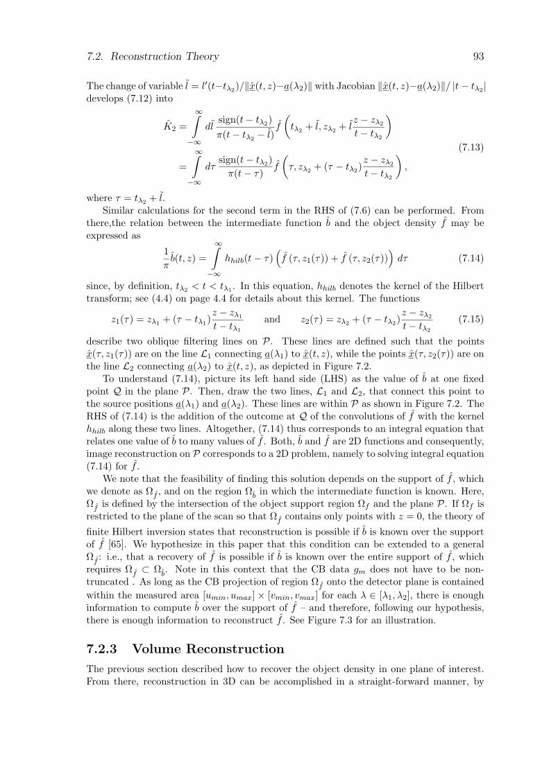
7.2. Reconstruction Theory 93
The change of variable l = l′(t−tλ2)/‖x(t, z)−a(λ2)‖ with Jacobian ‖x(t, z)−a(λ2)‖/ |t− tλ2 |develops (7.12) into
K2 =
∞∫
−∞dl
sign(t− tλ2)π(t− tλ2 − l)
f
(tλ2 + l, zλ2 + l
z − zλ2
t− tλ2
)
=
∞∫
−∞dτ
sign(t− tλ2)π(t− τ)
f
(τ, zλ2 + (τ − tλ2)
z − zλ2
t− tλ2
),
(7.13)
where τ = tλ2 + l.Similar calculations for the second term in the RHS of (7.6) can be performed. From
there,the relation between the intermediate function b and the object density f may beexpressed as
1π
b(t, z) =
∞∫
−∞hhilb(t− τ)
(f (τ, z1(τ)) + f (τ, z2(τ))
)dτ (7.14)
since, by definition, tλ2 < t < tλ1 . In this equation, hhilb denotes the kernel of the Hilberttransform; see (4.4) on page 4.4 for details about this kernel. The functions
z1(τ) = zλ1 + (τ − tλ1)z − zλ1
t− tλ1
and z2(τ) = zλ2 + (τ − tλ2)z − zλ2
t− tλ2
(7.15)
describe two oblique filtering lines on P. These lines are defined such that the pointsx(τ, z1(τ)) are on the line L1 connecting a(λ1) to x(t, z), while the points x(τ, z2(τ)) are onthe line L2 connecting a(λ2) to x(t, z), as depicted in Figure 7.2.
To understand (7.14), picture its left hand side (LHS) as the value of b at one fixedpoint Q in the plane P. Then, draw the two lines, L1 and L2, that connect this point tothe source positions a(λ1) and a(λ2). These lines are within P as shown in Figure 7.2. TheRHS of (7.14) is the addition of the outcome at Q of the convolutions of f with the kernelhhilb along these two lines. Altogether, (7.14) thus corresponds to an integral equation thatrelates one value of b to many values of f . Both, b and f are 2D functions and consequently,image reconstruction on P corresponds to a 2D problem, namely to solving integral equation(7.14) for f .
We note that the feasibility of finding this solution depends on the support of f , whichwe denote as Ωf , and on the region Ωb in which the intermediate function is known. Here,Ωf is defined by the intersection of the object support region Ωf and the plane P. If Ωf isrestricted to the plane of the scan so that Ωf contains only points with z = 0, the theory of
finite Hilbert inversion states that reconstruction is possible if b is known over the supportof f [65]. We hypothesize in this paper that this condition can be extended to a generalΩf : i.e., that a recovery of f is possible if b is known over the entire support of f , whichrequires Ωf ⊂ Ωb. Note in this context that the CB data gm does not have to be non-truncated . As long as the CB projection of region Ωf onto the detector plane is containedwithin the measured area [umin, umax] × [vmin, vmax] for each λ ∈ [λ1, λ2], there is enoughinformation to compute b over the support of f – and therefore, following our hypothesis,there is enough information to reconstruct f . See Figure 7.3 for an illustration.
7.2.3 Volume Reconstruction
The previous section described how to recover the object density in one plane of interest.From there, reconstruction in 3D can be accomplished in a straight-forward manner, by
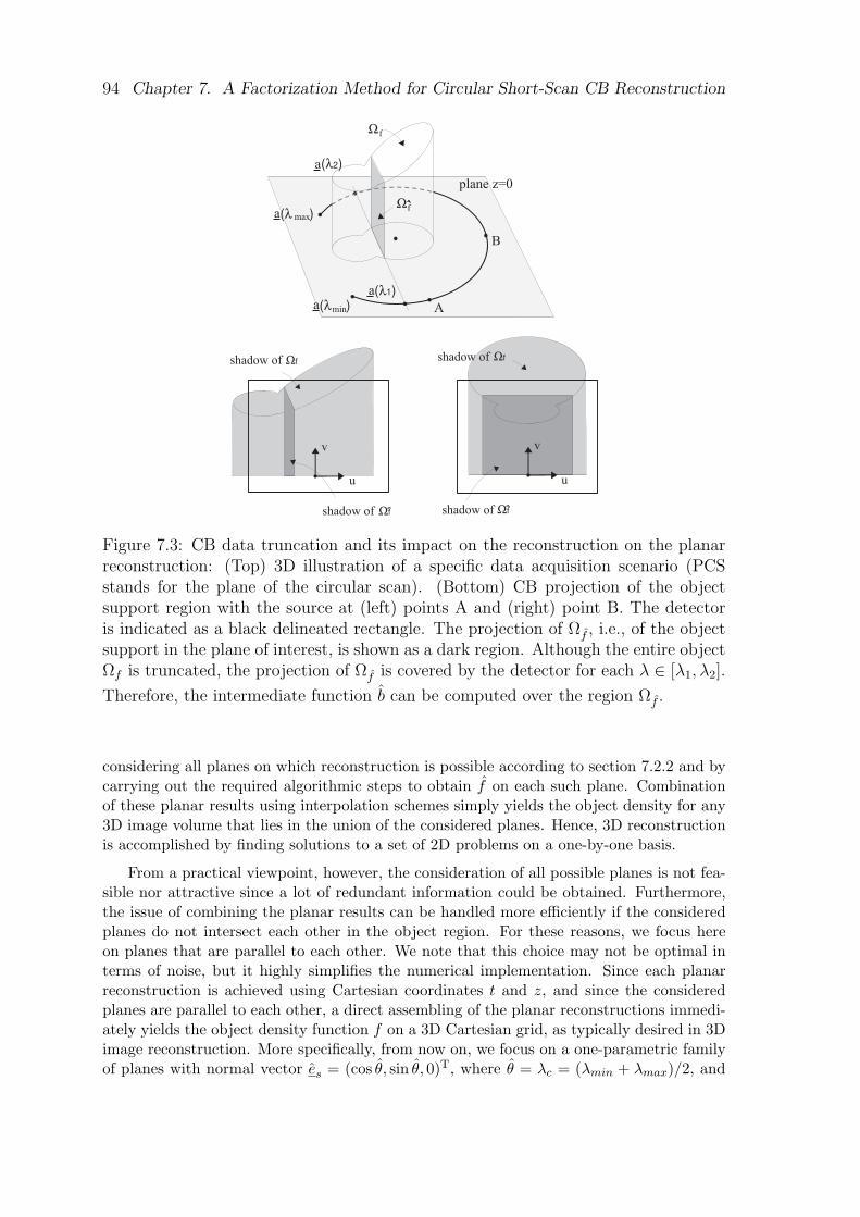
94 Chapter 7. A Factorization Method for Circular Short-Scan CB Reconstruction
plane z=0
B
Amin
max
a
f
aa
a
f
shadow of
u
v
shadow of
shadow of shadow of
u
v
Figure 7.3: CB data truncation and its impact on the reconstruction on the planarreconstruction: (Top) 3D illustration of a specific data acquisition scenario (PCSstands for the plane of the circular scan). (Bottom) CB projection of the objectsupport region with the source at (left) points A and (right) point B. The detectoris indicated as a black delineated rectangle. The projection of Ωf , i.e., of the objectsupport in the plane of interest, is shown as a dark region. Although the entire objectΩf is truncated, the projection of Ωf is covered by the detector for each λ ∈ [λ1, λ2].
Therefore, the intermediate function b can be computed over the region Ωf .
considering all planes on which reconstruction is possible according to section 7.2.2 and bycarrying out the required algorithmic steps to obtain f on each such plane. Combinationof these planar results using interpolation schemes simply yields the object density for any3D image volume that lies in the union of the considered planes. Hence, 3D reconstructionis accomplished by finding solutions to a set of 2D problems on a one-by-one basis.
From a practical viewpoint, however, the consideration of all possible planes is not fea-sible nor attractive since a lot of redundant information could be obtained. Furthermore,the issue of combining the planar results can be handled more efficiently if the consideredplanes do not intersect each other in the object region. For these reasons, we focus hereon planes that are parallel to each other. We note that this choice may not be optimal interms of noise, but it highly simplifies the numerical implementation. Since each planarreconstruction is achieved using Cartesian coordinates t and z, and since the consideredplanes are parallel to each other, a direct assembling of the planar reconstructions immedi-ately yields the object density function f on a 3D Cartesian grid, as typically desired in 3Dimage reconstruction. More specifically, from now on, we focus on a one-parametric familyof planes with normal vector es = (cos θ, sin θ, 0)T, where θ = λc = (λmin + λmax)/2, and
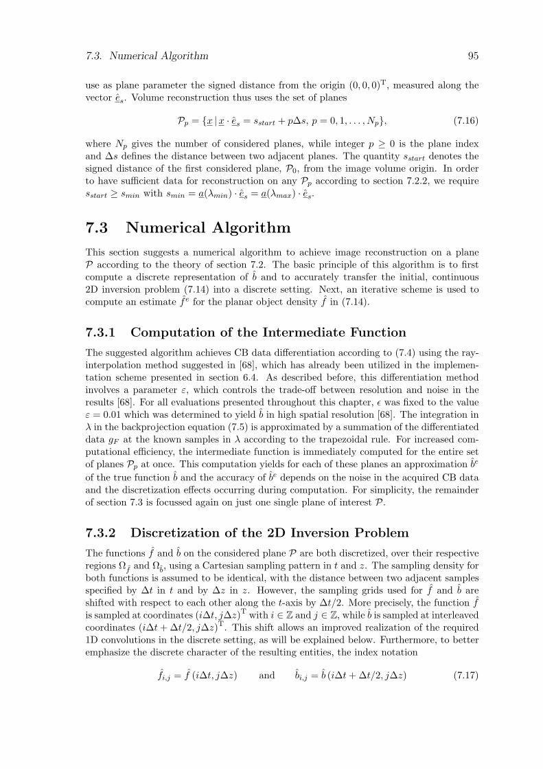
7.3. Numerical Algorithm 95
use as plane parameter the signed distance from the origin (0, 0, 0)T, measured along thevector es. Volume reconstruction thus uses the set of planes
Pp = x |x · es = sstart + p∆s, p = 0, 1, . . . , Np, (7.16)
where Np gives the number of considered planes, while integer p ≥ 0 is the plane indexand ∆s defines the distance between two adjacent planes. The quantity sstart denotes thesigned distance of the first considered plane, P0, from the image volume origin. In orderto have sufficient data for reconstruction on any Pp according to section 7.2.2, we requiresstart ≥ smin with smin = a(λmin) · es = a(λmax) · es.
7.3 Numerical Algorithm
This section suggests a numerical algorithm to achieve image reconstruction on a planeP according to the theory of section 7.2. The basic principle of this algorithm is to firstcompute a discrete representation of b and to accurately transfer the initial, continuous2D inversion problem (7.14) into a discrete setting. Next, an iterative scheme is used tocompute an estimate fe for the planar object density f in (7.14).
7.3.1 Computation of the Intermediate Function
The suggested algorithm achieves CB data differentiation according to (7.4) using the ray-interpolation method suggested in [68], which has already been utilized in the implemen-tation scheme presented in section 6.4. As described before, this differentiation methodinvolves a parameter ε, which controls the trade-off between resolution and noise in theresults [68]. For all evaluations presented throughout this chapter, ε was fixed to the valueε = 0.01 which was determined to yield b in high spatial resolution [68]. The integration inλ in the backprojection equation (7.5) is approximated by a summation of the differentiateddata gF at the known samples in λ according to the trapezoidal rule. For increased com-putational efficiency, the intermediate function is immediately computed for the entire setof planes Pp at once. This computation yields for each of these planes an approximation be
of the true function b and the accuracy of be depends on the noise in the acquired CB dataand the discretization effects occurring during computation. For simplicity, the remainderof section 7.3 is focussed again on just one single plane of interest P.
7.3.2 Discretization of the 2D Inversion Problem
The functions f and b on the considered plane P are both discretized, over their respectiveregions Ωf and Ωb, using a Cartesian sampling pattern in t and z. The sampling density forboth functions is assumed to be identical, with the distance between two adjacent samplesspecified by ∆t in t and by ∆z in z. However, the sampling grids used for f and b areshifted with respect to each other along the t-axis by ∆t/2. More precisely, the function fis sampled at coordinates (i∆t, j∆z)T with i ∈ Z and j ∈ Z, while b is sampled at interleavedcoordinates (i∆t + ∆t/2, j∆z)T. This shift allows an improved realization of the required1D convolutions in the discrete setting, as will be explained below. Furthermore, to betteremphasize the discrete character of the resulting entities, the index notation
fi,j = f (i∆t, j∆z) and bi,j = b (i∆t + ∆t/2, j∆z) (7.17)
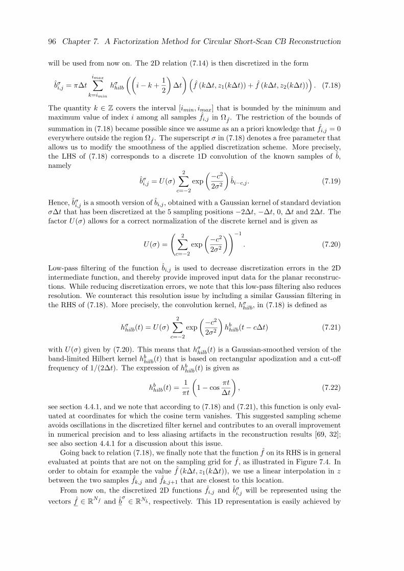
96 Chapter 7. A Factorization Method for Circular Short-Scan CB Reconstruction
will be used from now on. The 2D relation (7.14) is then discretized in the form
bσi,j = π∆t
imax∑
k=imin
hσhilb
((i− k +
12
)∆t
)(f (k∆t, z1(k∆t)) + f (k∆t, z2(k∆t))
). (7.18)
The quantity k ∈ Z covers the interval [imin, imax] that is bounded by the minimum andmaximum value of index i among all samples fi,j in Ωf . The restriction of the bounds of
summation in (7.18) became possible since we assume as an a priori knowledge that fi,j = 0everywhere outside the region Ωf . The superscript σ in (7.18) denotes a free parameter thatallows us to modify the smoothness of the applied discretization scheme. More precisely,the LHS of (7.18) corresponds to a discrete 1D convolution of the known samples of b,namely
bσi,j = U(σ)
2∑
c=−2
exp(−c2
2σ2
)bi−c,j . (7.19)
Hence, bσi,j is a smooth version of bi,j , obtained with a Gaussian kernel of standard deviation
σ∆t that has been discretized at the 5 sampling positions −2∆t, −∆t, 0, ∆t and 2∆t. Thefactor U(σ) allows for a correct normalization of the discrete kernel and is given as
U(σ) =
(2∑
c=−2
exp(−c2
2σ2
))−1
. (7.20)
Low-pass filtering of the function bi,j is used to decrease discretization errors in the 2Dintermediate function, and thereby provide improved input data for the planar reconstruc-tions. While reducing discretization errors, we note that this low-pass filtering also reducesresolution. We counteract this resolution issue by including a similar Gaussian filtering inthe RHS of (7.18). More precisely, the convolution kernel, hσ
hilb, in (7.18) is defined as
hσhilb(t) = U(σ)
2∑
c=−2
exp(−c2
2σ2
)hb
hilb(t− c∆t) (7.21)
with U(σ) given by (7.20). This means that hσhilb(t) is a Gaussian-smoothed version of the
band-limited Hilbert kernel hbhilb(t) that is based on rectangular apodization and a cut-off
frequency of 1/(2∆t). The expression of hbhilb(t) is given as
hbhilb(t) =
1πt
(1− cos
πt
∆t
), (7.22)
see section 4.4.1, and we note that according to (7.18) and (7.21), this function is only eval-uated at coordinates for which the cosine term vanishes. This suggested sampling schemeavoids oscillations in the discretized filter kernel and contributes to an overall improvementin numerical precision and to less aliasing artifacts in the reconstruction results [69, 32];see also section 4.4.1 for a discussion about this issue.
Going back to relation (7.18), we finally note that the function f on its RHS is in generalevaluated at points that are not on the sampling grid for f , as illustrated in Figure 7.4. Inorder to obtain for example the value f (k∆t, z1(k∆t)), we use a linear interpolation in zbetween the two samples fk,j and fk,j+1 that are closest to this location.
From now on, the discretized 2D functions fi,j and bσi,j will be represented using the
vectors f ∈ RNf and bσ ∈ RNb , respectively. This 1D representation is easily achieved by
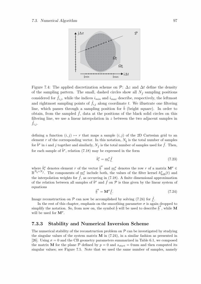
7.3. Numerical Algorithm 97
i t
f
b
z
min maxi i
j
Figure 7.4: The applied discretization scheme on P : ∆z and ∆t define the densityof the sampling pattern. The small, dashed circles show all Nf sampling positions
considered for fi,j, while the indices imin and imax describe, respectively, the leftmost
and rightmost sampling points of fi,j along coordinate t. We illustrate one filtering
line, which passes through a sampling position for b (bright square). In order toobtain, from the sampled f , data at the positions of the black solid circles on thisfiltering line, we use a linear interpolation in z between the two adjacent samples infi,j.
defining a function (i, j) 7→ r that maps a sample (i, j) of the 2D Cartesian grid to anelement r of the corresponding vector. In this notation, Nb is the total number of samplesfor bσ in i and j together and similarly, Nf is the total number of samples used for f . Then,
for each sample of bσ, relation (7.18) may be expressed in the form
bσr = mσ
r f (7.23)
where bσr denotes element r of the vector b
σand mσ
r denotes the row r of a matrix Mσ ∈RNb×Nf . The components of mσ
r include both, the values of the filter kernel hσhilb(t) and
the interpolation weights for f , as occurring in (7.18). A finite dimensional approximationof the relation between all samples of bσ and f on P is thus given by the linear system ofequations
bσ
= Mσf . (7.24)
Image reconstruction on P can now be accomplished by solving (7.24) for f .In the rest of this chapter, emphasis on the smoothing parameter σ is again dropped to
simplify the notation. So, from now on, the symbol b will be used to describe bσ, while M
will be used for Mσ.
7.3.3 Stability and Numerical Inversion Scheme
The numerical stability of the reconstruction problem on P can be investigated by studyingthe singular values of the system matrix M in (7.24), in a similar fashion as presented in[26]. Using σ = 0 and the CB geometry parameters summarized in Table 6.1, we composedthe matrix M for the plane P defined by p = 0 and sstart = 0 mm and then computed itssingular values; see Figure 7.5. Note that we used the same number of samples, namely
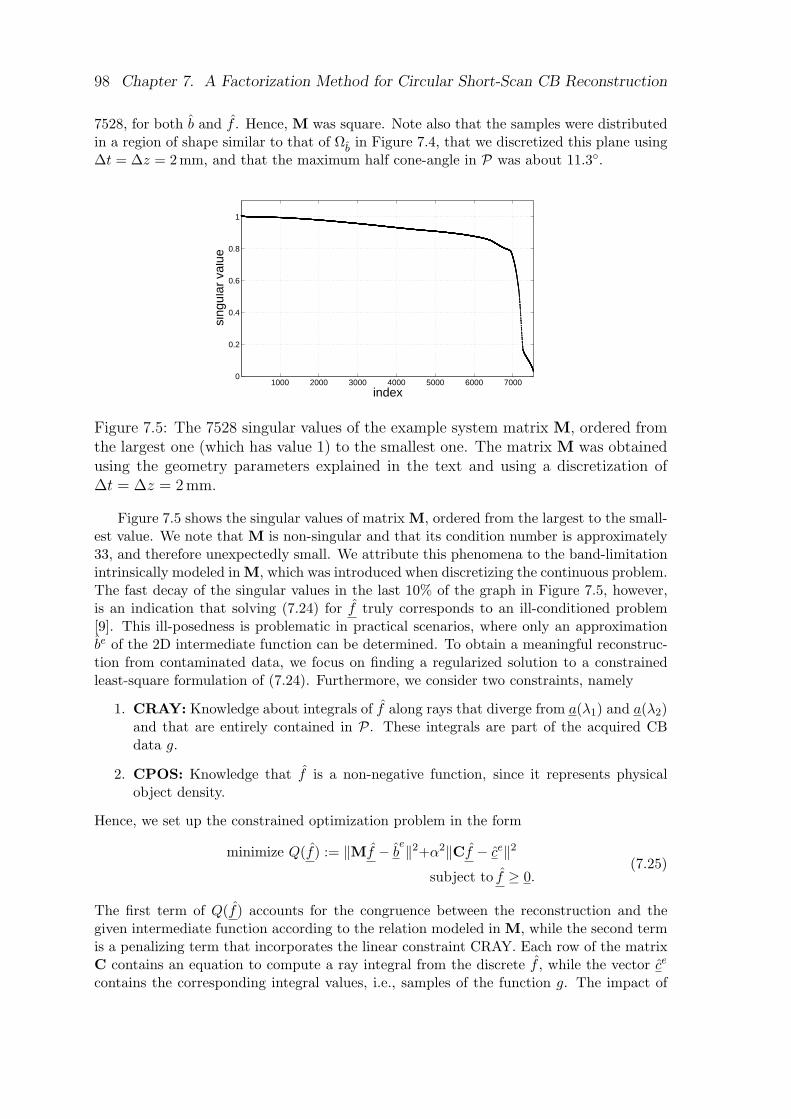
98 Chapter 7. A Factorization Method for Circular Short-Scan CB Reconstruction
7528, for both b and f . Hence, M was square. Note also that the samples were distributedin a region of shape similar to that of Ωb in Figure 7.4, that we discretized this plane using∆t = ∆z = 2mm, and that the maximum half cone-angle in P was about 11.3.
1000 2000 3000 4000 5000 6000 70000
0.2
0.4
0.6
0.8
1si
ngul
ar v
alue
index
Figure 7.5: The 7528 singular values of the example system matrix M, ordered fromthe largest one (which has value 1) to the smallest one. The matrix M was obtainedusing the geometry parameters explained in the text and using a discretization of∆t = ∆z = 2 mm.
Figure 7.5 shows the singular values of matrix M, ordered from the largest to the small-est value. We note that M is non-singular and that its condition number is approximately33, and therefore unexpectedly small. We attribute this phenomena to the band-limitationintrinsically modeled in M, which was introduced when discretizing the continuous problem.The fast decay of the singular values in the last 10% of the graph in Figure 7.5, however,is an indication that solving (7.24) for f truly corresponds to an ill-conditioned problem[9]. This ill-posedness is problematic in practical scenarios, where only an approximationbe of the 2D intermediate function can be determined. To obtain a meaningful reconstruc-tion from contaminated data, we focus on finding a regularized solution to a constrainedleast-square formulation of (7.24). Furthermore, we consider two constraints, namely
1. CRAY: Knowledge about integrals of f along rays that diverge from a(λ1) and a(λ2)and that are entirely contained in P. These integrals are part of the acquired CBdata g.
2. CPOS: Knowledge that f is a non-negative function, since it represents physicalobject density.
Hence, we set up the constrained optimization problem in the form
minimize Q(f) := ‖Mf − be‖2+α2‖Cf − ce‖2
subject to f ≥ 0.(7.25)
The first term of Q(f) accounts for the congruence between the reconstruction and thegiven intermediate function according to the relation modeled in M, while the second termis a penalizing term that incorporates the linear constraint CRAY. Each row of the matrixC contains an equation to compute a ray integral from the discrete f , while the vector ce
contains the corresponding integral values, i.e., samples of the function g. The impact of
7.3. Numerical Algorithm 99
CRAY may be adjusted using parameter α. We note that finding an appropriate value forα is a difficult problem, which will be addressed in more details in section 7.4.2.
To simplify the notation for the remainder of this section, the objective function in(7.25) may be expressed equivalently as
Q(f) = ‖Af − de‖2
= fTATAf − 2f
TATd
e+ d
eTd
e,
(7.26)
where
A =[
MαC
]and d
e=
[be
α ce
]. (7.27)
The solution of (7.25) is estimated using a projected steepest descent iteration scheme
[61, 16], during which a sequence of intermediate estimates f(q) ∈ RNf with integer iteration
index q ≥ 0 is computed. The initial estimate is set to f(0)
= 0 and the updating equationis
f(q+1)
= C(f
(q)+ w(q)u(q)
), (7.28)
using the update directionu(q) = −∇Q(f
(q)) (7.29)
with the gradient of Q(f) given as
∇Q(f) = 2AT(Af − de) (7.30)
and using the update step-width
w(q) =12‖u(q)‖2
‖Au(q)‖22
. (7.31)
To understand the scheme described by (7.28) to (7.31), note that in each iteration, f(q)
is first updated in the direction of the steepest descent of the quadratic functional Q atpoint f
(q), which is a natural selection when pursuing minimization. The update step-
width according to (7.31) guarantees that f(q)
+ w(q)u(q) minimizes Q on the line through
f(q)
with direction u(q) [16]. The operator C in (7.28) describes the orthogonal projectiononto the convex set of vectors with nonnegative entries. This projection assures that eachintermediate estimate satisfies the nonlinear constraint CPOS.
It can be shown that the sequence f(q)
converges towards the solution of (7.25) forincreasing q [45]. However, at some point during the iterations, the intermediate estimatemay start diverging from the true, desired, f due to contaminations in the data vector d
e.
We want to avoid this behavior and therefore suggest to stop iterations early, when eitherof the two following conditions is satisfied:
1. The iteration index q reaches a pre-defined maximum number γmax.
2. The value∥∥∥f
(q) − f(q−1)
∥∥∥∞
(with ‖ · ‖∞ denoting the maximum norm) first becomes
equal or less than a certain threshold. This threshold is here defined as γthres
∥∥∥f(q)
∥∥∥∞
,i.e., relative to the norm of the current intermediate estimate.
100 Chapter 7. A Factorization Method for Circular Short-Scan CB Reconstruction
Thus, iteration continues up to the maximum index γmax if at least one element of theintermediate estimate is still updated strongly enough, even if the update in all otherelements is already below the introduced threshold. Note that there exists a number ofindications that the early stopping rule applied to our steepest descent iteration schemeasymptotically defines a regularization process [63], as discussed in [9, 91].
Let Nq denote the iteration index at which the stopping criterion is satisfied. We define
fe
:= f(Nq)
(7.32)
as the nonnegative approximation to the solution of the constrained optimization problem(7.25) and consider f
eas a good estimate for the vector f that satisfies (7.24). The inverse
of the mapping defined earlier in this section, r 7→ (i, j), yields fei,j from f
eand therefore a
discrete 2D representation of the reconstructed object density on P, as desired.
7.4 Numerical Studies
This section presents an evaluation of the factorization method, based on CB data simulatedin the C-arm geometry (as defined previously in table 6.1). During data simulation, we madesure that the CB projection of the object support region Ωf onto the detector plane wasalways entirely contained in the measured area [umin, umax]× [vmin, vmax].
7.4.1 Experimental Set-Up
The experiments in this section involve two mathematical phantoms. The first one is a high-contrast disk phantom that consists of six cylindrical disks embedded in a low-attenuatingcylinder of radius 100 mm and density −900HU. Each disk has a thickness of 10 mm, aradius of 80mm and the density of water (defined as µwater = 0.01836mm−1). The disksare centered on the z-axis and stacked one above the other with a center-to-center distanceof 20 mm between any two adjacent disks. The first disk was centered on the plane of thesource trajectory and therefore, all other disks were above that plane. The second phantomwe use in this chapter is the FORBILD head phantom [3]. In the presented evaluations, thehead phantom was positioned so that its center is 40mm above the plane of the circularscan.
As described in section 7.3, the iterative inversion algorithm that we use for each planarreconstruction involves the selection of 4 parameters: α, σ, γthres and γmax. We herestudy in details the impacts of parameters α and σ on achievable reconstruction quality, byinvestigating the results obtained on a single plane of interest. Unless otherwise stated, afixed stopping rule was used, and this rule was defined with γthres = 0.002 and γmax = 400.
7.4.2 Impact of Parameter α on Image Quality
The effects of α on image quality are studied by reconstructing the disk phantom for arange of values of α while using the discretization ∆t = ∆z = 0.5 mm. The plane P onwhich reconstruction was achieved was defined with sstart = 0 mm, p = 0 and we set σ = 0.
The reconstruction results were evaluated quantitatively by computing as a FOM, i.e.,as a figure of merit, the root-mean-squared error (RMSE) between reconstruction fe andthe true object density f within two different regions in P. These regions, denoted as Aand B, were rectangular with width 100 mm and height 6mm and were entirely contained,
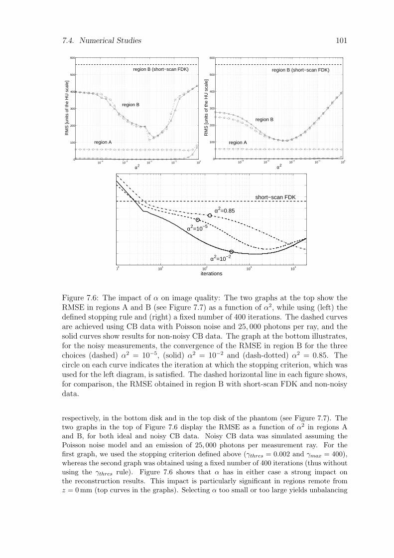
7.4. Numerical Studies 101
10−4
10−3
10−2
10−1
100
0
100
200
300
400
500
600
α2
RM
S [u
nits
of t
he H
U s
cale
]
region A
region B (short−scan FDK)
region B
10−4
10−3
10−2
10−1
100
0
100
200
300
400
500
600
α2
RM
S [u
nits
of t
he H
U s
cale
]
region A
region B
region B (short−scan FDK)
100
101
102
103
104
0
100
200
300
400
500
600
700
800
iterations
α2=10−2
α2=10−5
α2=0.85
short−scan FDK
Figure 7.6: The impact of α on image quality: The two graphs at the top show theRMSE in regions A and B (see Figure 7.7) as a function of α2, while using (left) thedefined stopping rule and (right) a fixed number of 400 iterations. The dashed curvesare achieved using CB data with Poisson noise and 25, 000 photons per ray, and thesolid curves show results for non-noisy CB data. The graph at the bottom illustrates,for the noisy measurements, the convergence of the RMSE in region B for the threechoices (dashed) α2 = 10−5, (solid) α2 = 10−2 and (dash-dotted) α2 = 0.85. Thecircle on each curve indicates the iteration at which the stopping criterion, which wasused for the left diagram, is satisfied. The dashed horizontal line in each figure shows,for comparison, the RMSE obtained in region B with short-scan FDK and non-noisydata.
respectively, in the bottom disk and in the top disk of the phantom (see Figure 7.7). Thetwo graphs in the top of Figure 7.6 display the RMSE as a function of α2 in regions Aand B, for both ideal and noisy CB data. Noisy CB data was simulated assuming thePoisson noise model and an emission of 25, 000 photons per measurement ray. For thefirst graph, we used the stopping criterion defined above (γthres = 0.002 and γmax = 400),whereas the second graph was obtained using a fixed number of 400 iterations (thus withoutusing the γthres rule). Figure 7.6 shows that α has in either case a strong impact onthe reconstruction results. This impact is particularly significant in regions remote fromz = 0 mm (top curves in the graphs). Selecting α too small or too large yields unbalancing
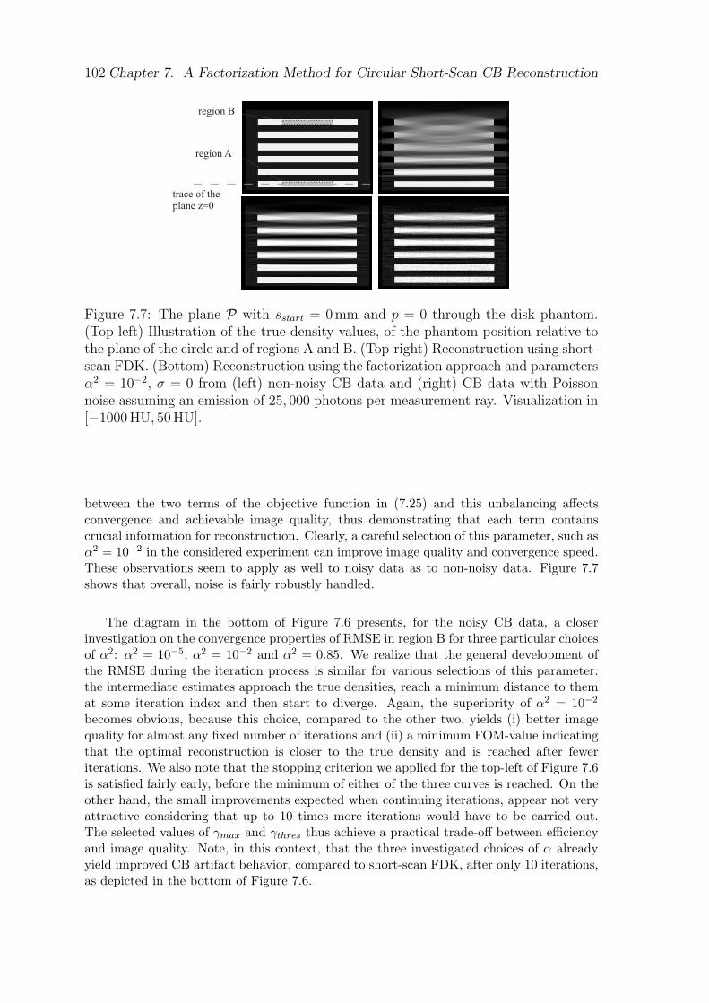
102 Chapter 7. A Factorization Method for Circular Short-Scan CB Reconstruction
region B
region A
trace of theplane z=0
Figure 7.7: The plane P with sstart = 0mm and p = 0 through the disk phantom.(Top-left) Illustration of the true density values, of the phantom position relative tothe plane of the circle and of regions A and B. (Top-right) Reconstruction using short-scan FDK. (Bottom) Reconstruction using the factorization approach and parametersα2 = 10−2, σ = 0 from (left) non-noisy CB data and (right) CB data with Poissonnoise assuming an emission of 25, 000 photons per measurement ray. Visualization in[−1000 HU, 50 HU].
between the two terms of the objective function in (7.25) and this unbalancing affectsconvergence and achievable image quality, thus demonstrating that each term containscrucial information for reconstruction. Clearly, a careful selection of this parameter, such asα2 = 10−2 in the considered experiment can improve image quality and convergence speed.These observations seem to apply as well to noisy data as to non-noisy data. Figure 7.7shows that overall, noise is fairly robustly handled.
The diagram in the bottom of Figure 7.6 presents, for the noisy CB data, a closerinvestigation on the convergence properties of RMSE in region B for three particular choicesof α2: α2 = 10−5, α2 = 10−2 and α2 = 0.85. We realize that the general development ofthe RMSE during the iteration process is similar for various selections of this parameter:the intermediate estimates approach the true densities, reach a minimum distance to themat some iteration index and then start to diverge. Again, the superiority of α2 = 10−2
becomes obvious, because this choice, compared to the other two, yields (i) better imagequality for almost any fixed number of iterations and (ii) a minimum FOM-value indicatingthat the optimal reconstruction is closer to the true density and is reached after feweriterations. We also note that the stopping criterion we applied for the top-left of Figure 7.6is satisfied fairly early, before the minimum of either of the three curves is reached. On theother hand, the small improvements expected when continuing iterations, appear not veryattractive considering that up to 10 times more iterations would have to be carried out.The selected values of γmax and γthres thus achieve a practical trade-off between efficiencyand image quality. Note, in this context, that the three investigated choices of α alreadyyield improved CB artifact behavior, compared to short-scan FDK, after only 10 iterations,as depicted in the bottom of Figure 7.6.
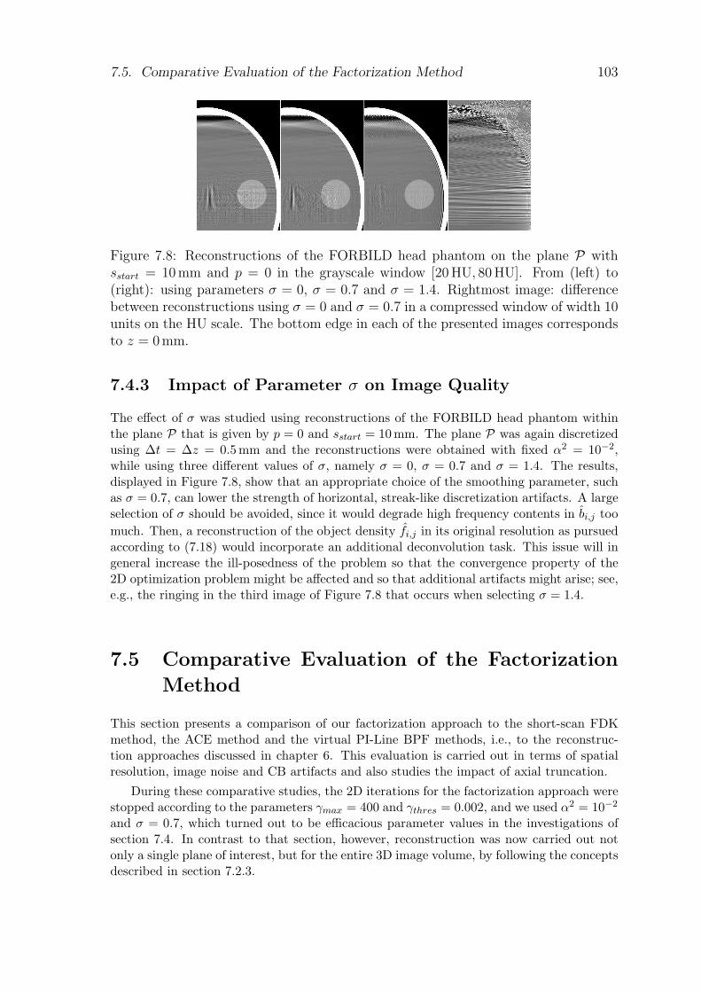
7.5. Comparative Evaluation of the Factorization Method 103
Figure 7.8: Reconstructions of the FORBILD head phantom on the plane P withsstart = 10mm and p = 0 in the grayscale window [20 HU, 80 HU]. From (left) to(right): using parameters σ = 0, σ = 0.7 and σ = 1.4. Rightmost image: differencebetween reconstructions using σ = 0 and σ = 0.7 in a compressed window of width 10units on the HU scale. The bottom edge in each of the presented images correspondsto z = 0mm.
7.4.3 Impact of Parameter σ on Image Quality
The effect of σ was studied using reconstructions of the FORBILD head phantom withinthe plane P that is given by p = 0 and sstart = 10 mm. The plane P was again discretizedusing ∆t = ∆z = 0.5mm and the reconstructions were obtained with fixed α2 = 10−2,while using three different values of σ, namely σ = 0, σ = 0.7 and σ = 1.4. The results,displayed in Figure 7.8, show that an appropriate choice of the smoothing parameter, suchas σ = 0.7, can lower the strength of horizontal, streak-like discretization artifacts. A largeselection of σ should be avoided, since it would degrade high frequency contents in bi,j toomuch. Then, a reconstruction of the object density fi,j in its original resolution as pursuedaccording to (7.18) would incorporate an additional deconvolution task. This issue will ingeneral increase the ill-posedness of the problem so that the convergence property of the2D optimization problem might be affected and so that additional artifacts might arise; see,e.g., the ringing in the third image of Figure 7.8 that occurs when selecting σ = 1.4.
7.5 Comparative Evaluation of the Factorization
Method
This section presents a comparison of our factorization approach to the short-scan FDKmethod, the ACE method and the virtual PI-Line BPF methods, i.e., to the reconstruc-tion approaches discussed in chapter 6. This evaluation is carried out in terms of spatialresolution, image noise and CB artifacts and also studies the impact of axial truncation.
During these comparative studies, the 2D iterations for the factorization approach werestopped according to the parameters γmax = 400 and γthres = 0.002, and we used α2 = 10−2
and σ = 0.7, which turned out to be efficacious parameter values in the investigations ofsection 7.4. In contrast to that section, however, reconstruction was now carried out notonly a single plane of interest, but for the entire 3D image volume, by following the conceptsdescribed in section 7.2.3.
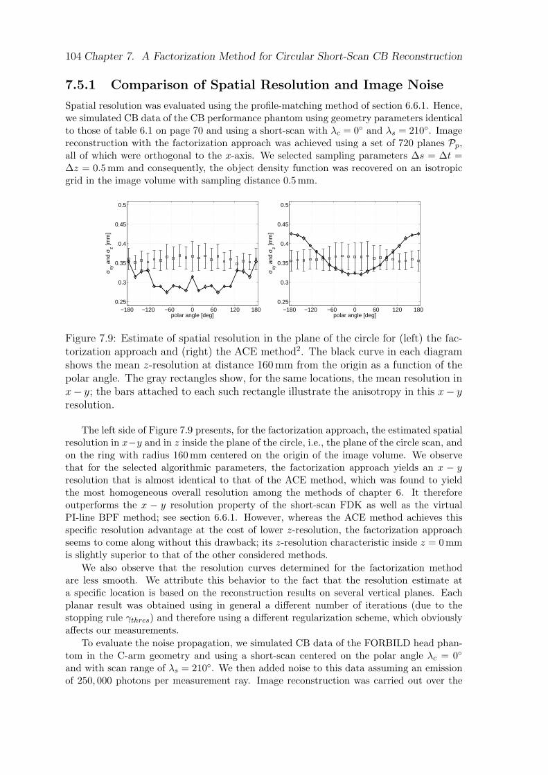
104 Chapter 7. A Factorization Method for Circular Short-Scan CB Reconstruction
7.5.1 Comparison of Spatial Resolution and Image Noise
Spatial resolution was evaluated using the profile-matching method of section 6.6.1. Hence,we simulated CB data of the CB performance phantom using geometry parameters identicalto those of table 6.1 on page 70 and using a short-scan with λc = 0 and λs = 210. Imagereconstruction with the factorization approach was achieved using a set of 720 planes Pp,all of which were orthogonal to the x-axis. We selected sampling parameters ∆s = ∆t =∆z = 0.5mm and consequently, the object density function was recovered on an isotropicgrid in the image volume with sampling distance 0.5mm.
−180 −120 −60 0 60 120 1800.25
0.3
0.35
0.4
0.45
0.5
polar angle [deg]
σ xy a
nd σ
z [mm
]
−180 −120 −60 0 60 120 1800.25
0.3
0.35
0.4
0.45
0.5
polar angle [deg]
σ xy a
nd σ
z [mm
]
Figure 7.9: Estimate of spatial resolution in the plane of the circle for (left) the fac-torization approach and (right) the ACE method2. The black curve in each diagramshows the mean z-resolution at distance 160mm from the origin as a function of thepolar angle. The gray rectangles show, for the same locations, the mean resolution inx− y; the bars attached to each such rectangle illustrate the anisotropy in this x− yresolution.
The left side of Figure 7.9 presents, for the factorization approach, the estimated spatialresolution in x−y and in z inside the plane of the circle, i.e., the plane of the circle scan, andon the ring with radius 160 mm centered on the origin of the image volume. We observethat for the selected algorithmic parameters, the factorization approach yields an x − yresolution that is almost identical to that of the ACE method, which was found to yieldthe most homogeneous overall resolution among the methods of chapter 6. It thereforeoutperforms the x − y resolution property of the short-scan FDK as well as the virtualPI-line BPF method; see section 6.6.1. However, whereas the ACE method achieves thisspecific resolution advantage at the cost of lower z-resolution, the factorization approachseems to come along without this drawback; its z-resolution characteristic inside z = 0mmis slightly superior to that of the other considered methods.
We also observe that the resolution curves determined for the factorization methodare less smooth. We attribute this behavior to the fact that the resolution estimate ata specific location is based on the reconstruction results on several vertical planes. Eachplanar result was obtained using in general a different number of iterations (due to thestopping rule γthres) and therefore using a different regularization scheme, which obviouslyaffects our measurements.
To evaluate the noise propagation, we simulated CB data of the FORBILD head phan-tom in the C-arm geometry and using a short-scan centered on the polar angle λc = 0
and with scan range of λs = 210. We then added noise to this data assuming an emissionof 250, 000 photons per measurement ray. Image reconstruction was carried out over the
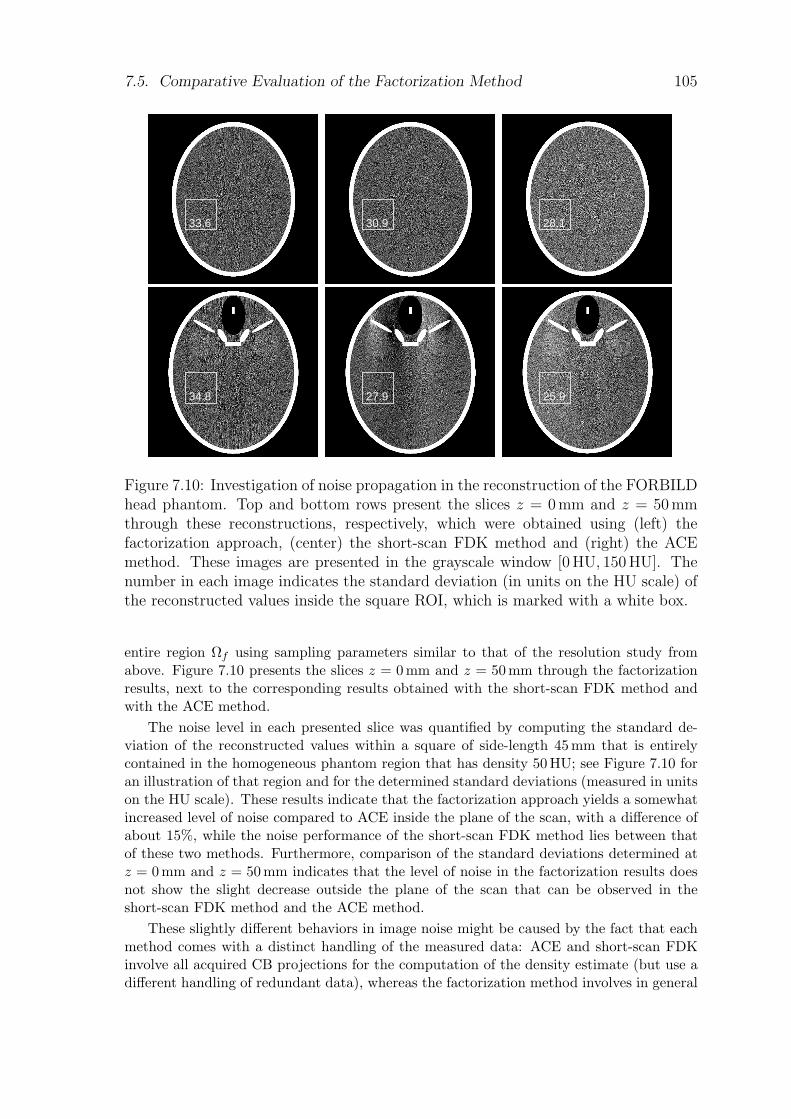
7.5. Comparative Evaluation of the Factorization Method 105
33.6 30.9 28.1
34.8 27.9 25.9
Figure 7.10: Investigation of noise propagation in the reconstruction of the FORBILDhead phantom. Top and bottom rows present the slices z = 0mm and z = 50mmthrough these reconstructions, respectively, which were obtained using (left) thefactorization approach, (center) the short-scan FDK method and (right) the ACEmethod. These images are presented in the grayscale window [0 HU, 150 HU]. Thenumber in each image indicates the standard deviation (in units on the HU scale) ofthe reconstructed values inside the square ROI, which is marked with a white box.
entire region Ωf using sampling parameters similar to that of the resolution study fromabove. Figure 7.10 presents the slices z = 0 mm and z = 50 mm through the factorizationresults, next to the corresponding results obtained with the short-scan FDK method andwith the ACE method.
The noise level in each presented slice was quantified by computing the standard de-viation of the reconstructed values within a square of side-length 45 mm that is entirelycontained in the homogeneous phantom region that has density 50 HU; see Figure 7.10 foran illustration of that region and for the determined standard deviations (measured in unitson the HU scale). These results indicate that the factorization approach yields a somewhatincreased level of noise compared to ACE inside the plane of the scan, with a difference ofabout 15%, while the noise performance of the short-scan FDK method lies between thatof these two methods. Furthermore, comparison of the standard deviations determined atz = 0 mm and z = 50mm indicates that the level of noise in the factorization results doesnot show the slight decrease outside the plane of the scan that can be observed in theshort-scan FDK method and the ACE method.
These slightly different behaviors in image noise might be caused by the fact that eachmethod comes with a distinct handling of the measured data: ACE and short-scan FDKinvolve all acquired CB projections for the computation of the density estimate (but use adifferent handling of redundant data), whereas the factorization method involves in general
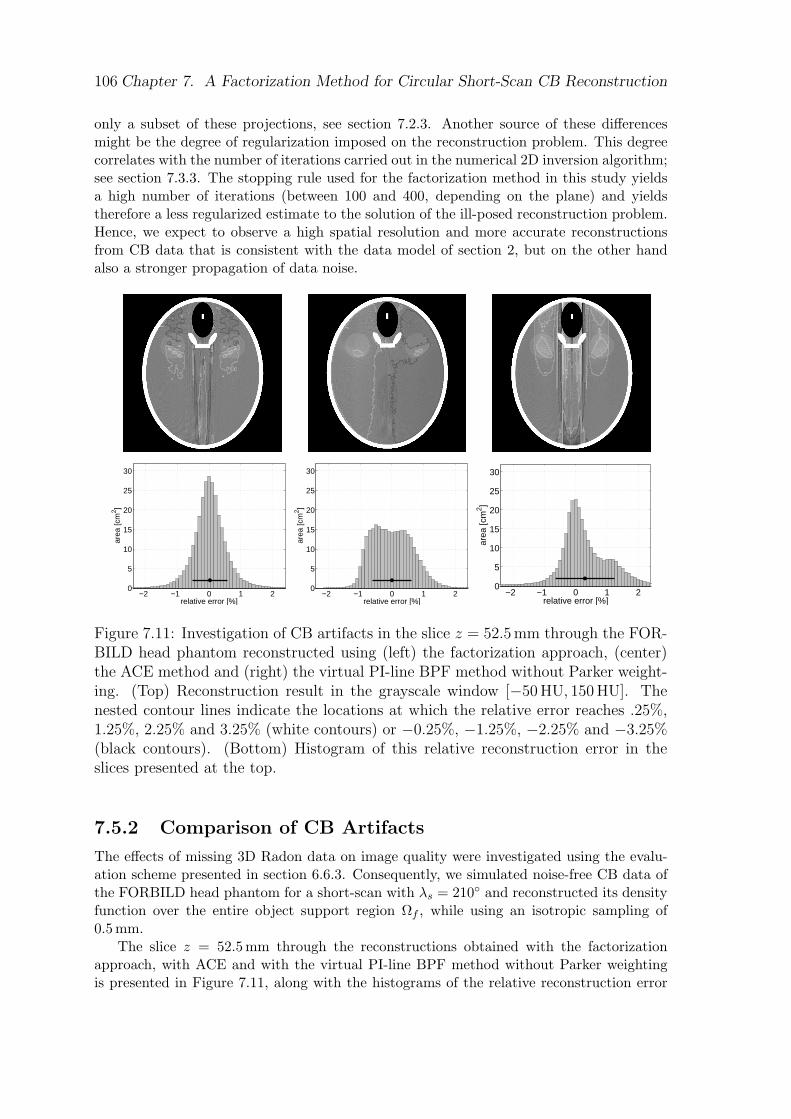
106 Chapter 7. A Factorization Method for Circular Short-Scan CB Reconstruction
only a subset of these projections, see section 7.2.3. Another source of these differencesmight be the degree of regularization imposed on the reconstruction problem. This degreecorrelates with the number of iterations carried out in the numerical 2D inversion algorithm;see section 7.3.3. The stopping rule used for the factorization method in this study yieldsa high number of iterations (between 100 and 400, depending on the plane) and yieldstherefore a less regularized estimate to the solution of the ill-posed reconstruction problem.Hence, we expect to observe a high spatial resolution and more accurate reconstructionsfrom CB data that is consistent with the data model of section 2, but on the other handalso a stronger propagation of data noise.
−2 −1 0 1 20
5
10
15
20
25
30
relative error [%]
area
[cm
2 ]
−2 −1 0 1 20
5
10
15
20
25
30
relative error [%]
area
[cm
2 ]
−2 −1 0 1 20
5
10
15
20
25
30
relative error [%]
area
[cm
2 ]
Figure 7.11: Investigation of CB artifacts in the slice z = 52.5mm through the FOR-BILD head phantom reconstructed using (left) the factorization approach, (center)the ACE method and (right) the virtual PI-line BPF method without Parker weight-ing. (Top) Reconstruction result in the grayscale window [−50 HU, 150 HU]. Thenested contour lines indicate the locations at which the relative error reaches .25%,1.25%, 2.25% and 3.25% (white contours) or −0.25%, −1.25%, −2.25% and −3.25%(black contours). (Bottom) Histogram of this relative reconstruction error in theslices presented at the top.
7.5.2 Comparison of CB Artifacts
The effects of missing 3D Radon data on image quality were investigated using the evalu-ation scheme presented in section 6.6.3. Consequently, we simulated noise-free CB data ofthe FORBILD head phantom for a short-scan with λs = 210 and reconstructed its densityfunction over the entire object support region Ωf , while using an isotropic sampling of0.5mm.
The slice z = 52.5mm through the reconstructions obtained with the factorizationapproach, with ACE and with the virtual PI-line BPF method without Parker weightingis presented in Figure 7.11, along with the histograms of the relative reconstruction error
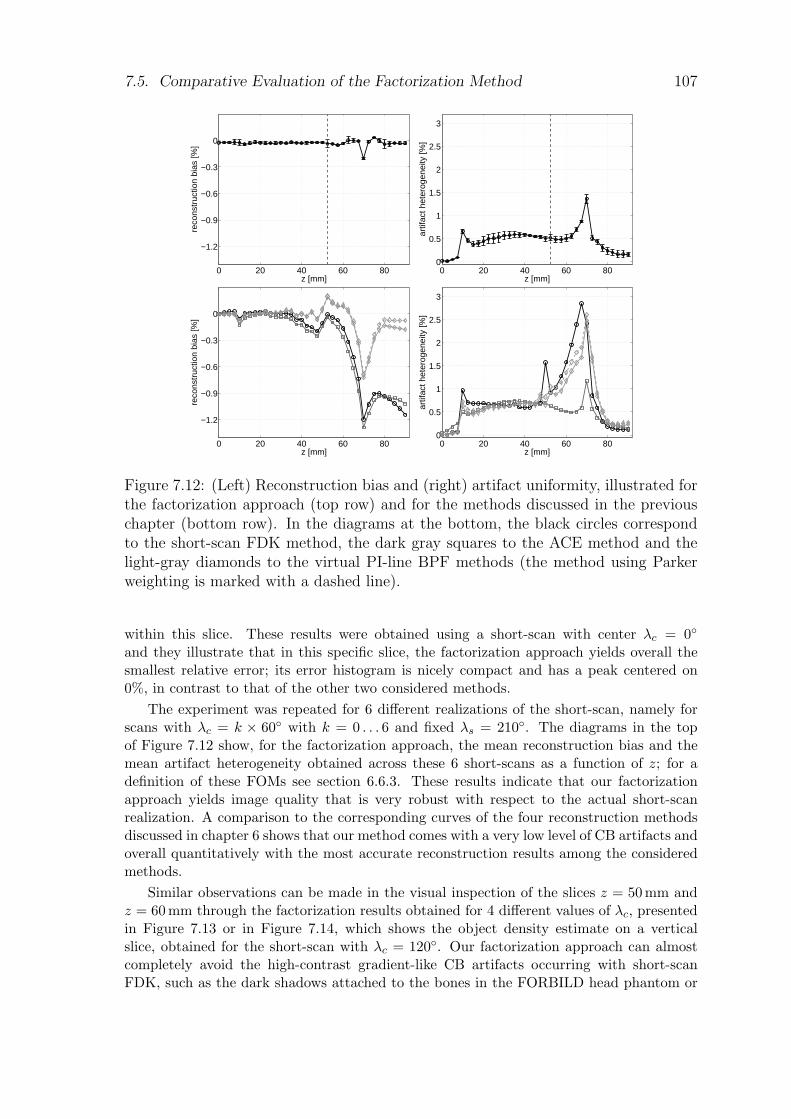
7.5. Comparative Evaluation of the Factorization Method 107
0 20 40 60 80
−1.2
−0.9
−0.6
−0.3
0
z [mm]
reco
nstr
uctio
n bi
as [%
]
0 20 40 60 800
0.5
1
1.5
2
2.5
3
z [mm]
artif
act h
eter
ogen
eity
[%]
0 20 40 60 80
−1.2
−0.9
−0.6
−0.3
0
z [mm]
reco
nstr
uctio
n bi
as [%
]
0 20 40 60 800
0.5
1
1.5
2
2.5
3
z [mm]
artif
act h
eter
ogen
eity
[%]
Figure 7.12: (Left) Reconstruction bias and (right) artifact uniformity, illustrated forthe factorization approach (top row) and for the methods discussed in the previouschapter (bottom row). In the diagrams at the bottom, the black circles correspondto the short-scan FDK method, the dark gray squares to the ACE method and thelight-gray diamonds to the virtual PI-line BPF methods (the method using Parkerweighting is marked with a dashed line).
within this slice. These results were obtained using a short-scan with center λc = 0
and they illustrate that in this specific slice, the factorization approach yields overall thesmallest relative error; its error histogram is nicely compact and has a peak centered on0%, in contrast to that of the other two considered methods.
The experiment was repeated for 6 different realizations of the short-scan, namely forscans with λc = k × 60 with k = 0 . . . 6 and fixed λs = 210. The diagrams in the topof Figure 7.12 show, for the factorization approach, the mean reconstruction bias and themean artifact heterogeneity obtained across these 6 short-scans as a function of z; for adefinition of these FOMs see section 6.6.3. These results indicate that our factorizationapproach yields image quality that is very robust with respect to the actual short-scanrealization. A comparison to the corresponding curves of the four reconstruction methodsdiscussed in chapter 6 shows that our method comes with a very low level of CB artifacts andoverall quantitatively with the most accurate reconstruction results among the consideredmethods.
Similar observations can be made in the visual inspection of the slices z = 50 mm andz = 60 mm through the factorization results obtained for 4 different values of λc, presentedin Figure 7.13 or in Figure 7.14, which shows the object density estimate on a verticalslice, obtained for the short-scan with λc = 120. Our factorization approach can almostcompletely avoid the high-contrast gradient-like CB artifacts occurring with short-scanFDK, such as the dark shadows attached to the bones in the FORBILD head phantom or
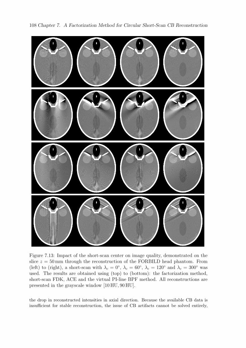
108 Chapter 7. A Factorization Method for Circular Short-Scan CB Reconstruction
Figure 7.13: Impact of the short-scan center on image quality, demonstrated on theslice z = 50mm through the reconstruction of the FORBILD head phantom. From(left) to (right), a short-scan with λc = 0, λc = 60, λc = 120 and λc = 300 wasused. The results are obtained using (top) to (bottom): the factorization method,short-scan FDK, ACE and the virtual PI-line BPF method. All reconstructions arepresented in the grayscale window [10 HU, 90 HU].
the drop in reconstructed intensities in axial direction. Because the available CB data isinsufficient for stable reconstruction, the issue of CB artifacts cannot be solved entirely,
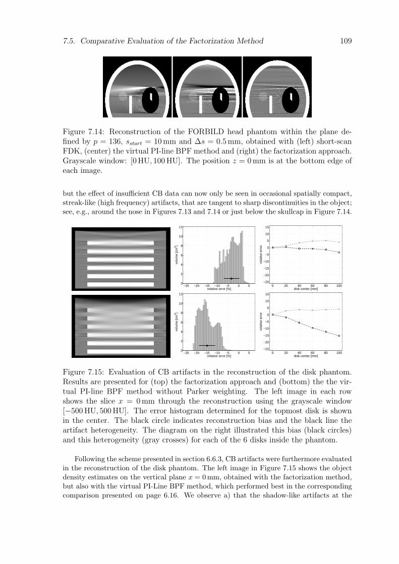
7.5. Comparative Evaluation of the Factorization Method 109
Figure 7.14: Reconstruction of the FORBILD head phantom within the plane de-fined by p = 136, sstart = 10mm and ∆s = 0.5mm, obtained with (left) short-scanFDK, (center) the virtual PI-line BPF method and (right) the factorization approach.Grayscale window: [0 HU, 100 HU]. The position z = 0mm is at the bottom edge ofeach image.
but the effect of insufficient CB data can now only be seen in occasional spatially compact,streak-like (high frequency) artifacts, that are tangent to sharp discontinuities in the object;see, e.g., around the nose in Figures 7.13 and 7.14 or just below the skullcap in Figure 7.14.
−25 −20 −15 −10 −5 0 50
2
4
6
8
10
12
relative error [%]
volu
me
[cm
3 ]
0 20 40 60 80 100−25
−20
−15
−10
−5
0
5
10
15
disk center [mm]
rela
tive
erro
r
−25 −20 −15 −10 −5 0 50
2
4
6
8
10
12
relative error [%]
volu
me
[cm
3 ]
0 20 40 60 80 100−25
−20
−15
−10
−5
0
5
10
15
disk center [mm]
rela
tive
erro
r
Figure 7.15: Evaluation of CB artifacts in the reconstruction of the disk phantom.Results are presented for (top) the factorization approach and (bottom) the the vir-tual PI-line BPF method without Parker weighting. The left image in each rowshows the slice x = 0mm through the reconstruction using the grayscale window[−500 HU, 500 HU]. The error histogram determined for the topmost disk is shownin the center. The black circle indicates reconstruction bias and the black line theartifact heterogeneity. The diagram on the right illustrated this bias (black circles)and this heterogeneity (gray crosses) for each of the 6 disks inside the phantom.
Following the scheme presented in section 6.6.3, CB artifacts were furthermore evaluatedin the reconstruction of the disk phantom. The left image in Figure 7.15 shows the objectdensity estimates on the vertical plane x = 0 mm, obtained with the factorization method,but also with the virtual PI-Line BPF method, which performed best in the correspondingcomparison presented on page 6.16. We observe a) that the shadow-like artifacts at the
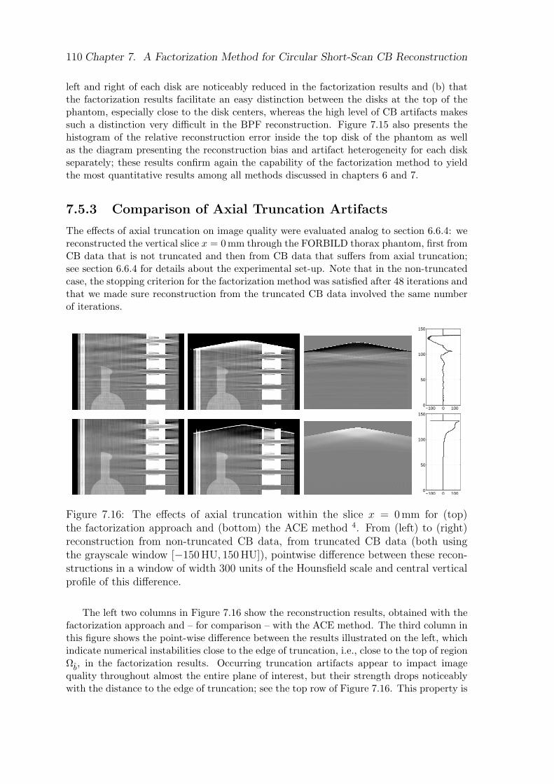
110 Chapter 7. A Factorization Method for Circular Short-Scan CB Reconstruction
left and right of each disk are noticeably reduced in the factorization results and (b) thatthe factorization results facilitate an easy distinction between the disks at the top of thephantom, especially close to the disk centers, whereas the high level of CB artifacts makessuch a distinction very difficult in the BPF reconstruction. Figure 7.15 also presents thehistogram of the relative reconstruction error inside the top disk of the phantom as wellas the diagram presenting the reconstruction bias and artifact heterogeneity for each diskseparately; these results confirm again the capability of the factorization method to yieldthe most quantitative results among all methods discussed in chapters 6 and 7.
7.5.3 Comparison of Axial Truncation Artifacts
The effects of axial truncation on image quality were evaluated analog to section 6.6.4: wereconstructed the vertical slice x = 0 mm through the FORBILD thorax phantom, first fromCB data that is not truncated and then from CB data that suffers from axial truncation;see section 6.6.4 for details about the experimental set-up. Note that in the non-truncatedcase, the stopping criterion for the factorization method was satisfied after 48 iterations andthat we made sure reconstruction from the truncated CB data involved the same numberof iterations.
−100 0 1000
50
100
150
−100 0 1000
50
100
150
Figure 7.16: The effects of axial truncation within the slice x = 0mm for (top)the factorization approach and (bottom) the ACE method 4. From (left) to (right)reconstruction from non-truncated CB data, from truncated CB data (both usingthe grayscale window [−150 HU, 150 HU]), pointwise difference between these recon-structions in a window of width 300 units of the Hounsfield scale and central verticalprofile of this difference.
The left two columns in Figure 7.16 show the reconstruction results, obtained with thefactorization approach and – for comparison – with the ACE method. The third column inthis figure shows the point-wise difference between the results illustrated on the left, whichindicate numerical instabilities close to the edge of truncation, i.e., close to the top of regionΩb, in the factorization results. Occurring truncation artifacts appear to impact imagequality throughout almost the entire plane of interest, but their strength drops noticeablywith the distance to the edge of truncation; see the top row of Figure 7.16. This property is
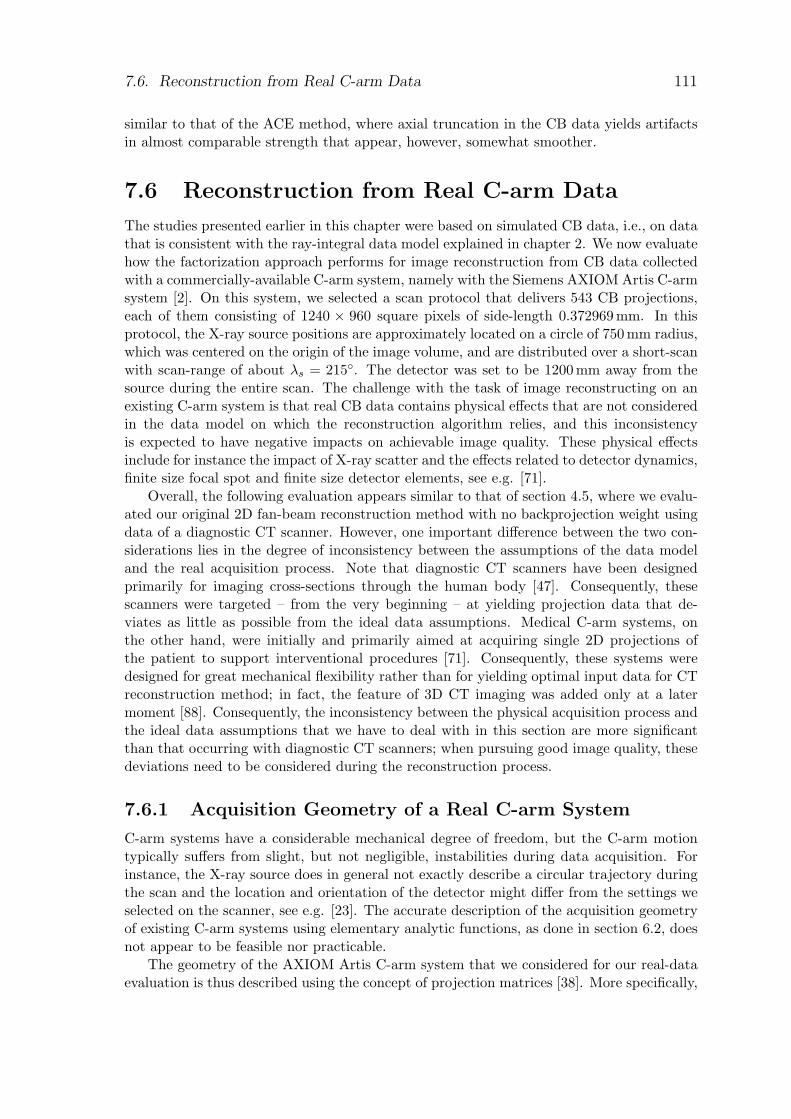
7.6. Reconstruction from Real C-arm Data 111
similar to that of the ACE method, where axial truncation in the CB data yields artifactsin almost comparable strength that appear, however, somewhat smoother.
7.6 Reconstruction from Real C-arm Data
The studies presented earlier in this chapter were based on simulated CB data, i.e., on datathat is consistent with the ray-integral data model explained in chapter 2. We now evaluatehow the factorization approach performs for image reconstruction from CB data collectedwith a commercially-available C-arm system, namely with the Siemens AXIOM Artis C-armsystem [2]. On this system, we selected a scan protocol that delivers 543 CB projections,each of them consisting of 1240 × 960 square pixels of side-length 0.372969 mm. In thisprotocol, the X-ray source positions are approximately located on a circle of 750 mm radius,which was centered on the origin of the image volume, and are distributed over a short-scanwith scan-range of about λs = 215. The detector was set to be 1200 mm away from thesource during the entire scan. The challenge with the task of image reconstructing on anexisting C-arm system is that real CB data contains physical effects that are not consideredin the data model on which the reconstruction algorithm relies, and this inconsistencyis expected to have negative impacts on achievable image quality. These physical effectsinclude for instance the impact of X-ray scatter and the effects related to detector dynamics,finite size focal spot and finite size detector elements, see e.g. [71].
Overall, the following evaluation appears similar to that of section 4.5, where we evalu-ated our original 2D fan-beam reconstruction method with no backprojection weight usingdata of a diagnostic CT scanner. However, one important difference between the two con-siderations lies in the degree of inconsistency between the assumptions of the data modeland the real acquisition process. Note that diagnostic CT scanners have been designedprimarily for imaging cross-sections through the human body [47]. Consequently, thesescanners were targeted – from the very beginning – at yielding projection data that de-viates as little as possible from the ideal data assumptions. Medical C-arm systems, onthe other hand, were initially and primarily aimed at acquiring single 2D projections ofthe patient to support interventional procedures [71]. Consequently, these systems weredesigned for great mechanical flexibility rather than for yielding optimal input data for CTreconstruction method; in fact, the feature of 3D CT imaging was added only at a latermoment [88]. Consequently, the inconsistency between the physical acquisition process andthe ideal data assumptions that we have to deal with in this section are more significantthan that occurring with diagnostic CT scanners; when pursuing good image quality, thesedeviations need to be considered during the reconstruction process.
7.6.1 Acquisition Geometry of a Real C-arm System
C-arm systems have a considerable mechanical degree of freedom, but the C-arm motiontypically suffers from slight, but not negligible, instabilities during data acquisition. Forinstance, the X-ray source does in general not exactly describe a circular trajectory duringthe scan and the location and orientation of the detector might differ from the settings weselected on the scanner, see e.g. [23]. The accurate description of the acquisition geometryof existing C-arm systems using elementary analytic functions, as done in section 6.2, doesnot appear to be feasible nor practicable.
The geometry of the AXIOM Artis C-arm system that we considered for our real-dataevaluation is thus described using the concept of projection matrices [38]. More specifically,
112 Chapter 7. A Factorization Method for Circular Short-Scan CB Reconstruction
the C-arm system associates, to each measured CB projection, one projection matrix Pi ∈R3×4 that describes, in homogeneous coordinates, the relation between a point x in theimage volume and the coordinates of its CB projection on the detector plane [88, 41],where the integer i corresponds to the index of the projection image. The matrix Pi encodescomplete information about the geometry parameters of the corresponding CB projection,such as the source position ai or the vectors eu,i, ev,i and ew,i. These parameters can beextracted from a given matrix Pi using the method described in [41].
Note that the sequence of projection matrices on the AXIOM Artis system are obtainedin a calibration step. This step is based on acquiring CB data of a specific calibration phan-tom, the structure of which is precisely known, and on estimating for the CB projection ithe matrix Pi that best describes the projection-relation between the known 3D structureof the calibration phantom and the acquired 2D image; for details see e.g. [41]. Fortunately,the deviations of the C-arm system from the ideal acquisition geometry are fairly repro-ducible so that for clinical use, the geometry information that is obtained in one calibrationstep may be used to geometrically describe the acquisition process of the subsequent scans.
7.6.2 Handling of Real C-arm CB Data
Recall that the factorization approach requires, as a first step, the partial differentiation ofthe CB data function g(λ, α) with respect to the curve parameter λ. This differentiationis a numerically delicate step, since (i) the sampling in λ of C-arm source trajectories isfairly coarse (compared the sampling of the trajectory for CT scanners) and (ii) the sourcetrajectory does not describe a simple geometric curve, due to mechanical instabilities. Ouralgorithm therefore applies the differentiation scheme introduced in [68] that is numericallyrobust with respect to coarse sampling and to arbitrary source motions. In particular, thisscheme was determined to yield an accurate differentiation results and to contribute to agood overall image quality in the context of C-arm reconstruction [40].
For the real-data reconstructions presented in the following (which are carried out usingan isotropic sampling of 0.5mm in the image volume), the differentiated CB data is down-sampled by a factor of 2 in u and in v, to reduce noise and to obtain a sampling in uand v that better matches the sampling grid defined for the image volume. The down-sampled differentiated CB projection with index i is then backprojected according to thegeometry parameters encoded in Pi. Note that the equations introduced on page 61 tocompute u∗ and v∗, i.e., the coordinates of the data samples required for reconstruction,involve simplifications that are based on the ideal geometry assumptions. Since the actualC-arm geometry does in general not satisfy these ideal assumptions, these equations arenow replaced by a more general form, and we compute the quantities u∗ and v∗ for the CBprojection i according to
u∗(x) = −D(x− ai) · eu,i
(x− ai) · ew,i
(7.33)
and
v∗(x) = −D(x− ai) · ev,i
(x− ai) · ew,i
(7.34)
respectively.To determine the values λ1 and λ2 that describe the points of intersection between the
source trajectory and the plane of interest P, which is described by its normal es and its
7.6. Reconstruction from Real C-arm Data 113
signed distance s from the image volume origin, we compute for each CB projection thequantity
ai · es − s, (7.35)
where ai is the source position extracted from the projection matrix Pi. Hence, (7.35)gives the signed distance of ai from P, measured along es. A positive value indicatesthat the source position for the CB projection with index i is between a(λ1) and a(λ2),so that according to (7.5) the corresponding filtered CB data is used for reconstructionon P. The CB projections with indices that result in a negative value in (7.35), however,are disregarded for reconstruction on P. CB projections at which (7.35) changes signare considered partially for the final reconstruction, with a weight that depends on thetrajectory discretization and the values computed in (7.35).
Finally, we make sure that the filtering lines involved in the 2D inversion process (forinstance the two lines L1 and L2 in the example of Figure 7.2) are constructed accurately andconsistent with the real acquisition geometry. This means that all these lines are constructedsuch that they pass through the actual intersection between the source trajectory and theplane P, which e.g. does not necessarily need to have z-coordinate z = 0 mm, as in theideal short-scan geometry.
7.6.3 Reconstruction Results
In the following, we illustrate the performance of the factorization approach including thealgorithmic modifications summarized in section 7.6.2 for reconstruction from real C-armCB data. For comparison, we show also the results obtained with the short-scan FDKalgorithm, i.e., the method used in state-of-the-art C-arm systems. Our short-scan FDKimplementation follows the scheme presented in section 6.3 but also considers algorithmicmodifications to handle the geometry deviations of C-arm systems. These modifications aresimilar to those explained in section 7.6.2 and are focussed on the accurate computation ofthe generalized Parker weighting function, of the backprojection weight and of the functionsu∗ and v∗ in the context of non-ideal geometries. Moreover, the acquired CB data is down-sampled by a factor of 2 in u and v before data filtering, as in the factorization method.
Figure 7.17: Reconstruction from the real C-arm data set A, obtained with (left)short-scan FDK and (right) the factorization approach. The results are presentedusing distinct grayscale-windows that were selected such that the mean of the recon-structed values in the small white rectangle has identical gray value in both images.
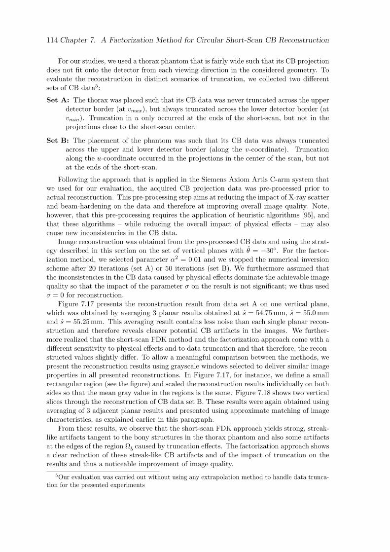
114 Chapter 7. A Factorization Method for Circular Short-Scan CB Reconstruction
For our studies, we used a thorax phantom that is fairly wide such that its CB projectiondoes not fit onto the detector from each viewing direction in the considered geometry. Toevaluate the reconstruction in distinct scenarios of truncation, we collected two differentsets of CB data5:
Set A: The thorax was placed such that its CB data was never truncated across the upperdetector border (at vmax), but always truncated across the lower detector border (atvmin). Truncation in u only occurred at the ends of the short-scan, but not in theprojections close to the short-scan center.
Set B: The placement of the phantom was such that its CB data was always truncatedacross the upper and lower detector border (along the v-coordinate). Truncationalong the u-coordinate occurred in the projections in the center of the scan, but notat the ends of the short-scan.
Following the approach that is applied in the Siemens Axiom Artis C-arm system thatwe used for our evaluation, the acquired CB projection data was pre-processed prior toactual reconstruction. This pre-processing step aims at reducing the impact of X-ray scatterand beam-hardening on the data and therefore at improving overall image quality. Note,however, that this pre-processing requires the application of heuristic algorithms [95], andthat these algorithms – while reducing the overall impact of physical effects – may alsocause new inconsistencies in the CB data.
Image reconstruction was obtained from the pre-processed CB data and using the strat-egy described in this section on the set of vertical planes with θ = −30. For the factor-ization method, we selected parameter α2 = 0.01 and we stopped the numerical inversionscheme after 20 iterations (set A) or 50 iterations (set B). We furthermore assumed thatthe inconsistencies in the CB data caused by physical effects dominate the achievable imagequality so that the impact of the parameter σ on the result is not significant; we thus usedσ = 0 for reconstruction.
Figure 7.17 presents the reconstruction result from data set A on one vertical plane,which was obtained by averaging 3 planar results obtained at s = 54.75 mm, s = 55.0mmand s = 55.25 mm. This averaging result contains less noise than each single planar recon-struction and therefore reveals clearer potential CB artifacts in the images. We further-more realized that the short-scan FDK method and the factorization approach come with adifferent sensitivity to physical effects and to data truncation and that therefore, the recon-structed values slightly differ. To allow a meaningful comparison between the methods, wepresent the reconstruction results using grayscale windows selected to deliver similar imageproperties in all presented reconstructions. In Figure 7.17, for instance, we define a smallrectangular region (see the figure) and scaled the reconstruction results individually on bothsides so that the mean gray value in the regions is the same. Figure 7.18 shows two verticalslices through the reconstruction of CB data set B. These results were again obtained usingaveraging of 3 adjacent planar results and presented using approximate matching of imagecharacteristics, as explained earlier in this paragraph.
From these results, we observe that the short-scan FDK approach yields strong, streak-like artifacts tangent to the bony structures in the thorax phantom and also some artifactsat the edges of the region Ωb caused by truncation effects. The factorization approach showsa clear reduction of these streak-like CB artifacts and of the impact of truncation on theresults and thus a noticeable improvement of image quality.
5Our evaluation was carried out without using any extrapolation method to handle data trunca-tion for the presented experiments
7.7. Discussion and Conclusions 115
Figure 7.18: Reconstruction from the real C-arm data set B, obtained with (left)short-scan FDK and (right) the factorization approach.
7.7 Discussion and Conclusions
As discussed in chapter 6, the problem of 3D CB image reconstruction in the short-scancircular acquisition geometry is known to be theoretically very challenging. Analyticalstate-of-the-art algorithms suggested to solve this problem all come with advantages anddisadvantages, as described before. For some imaging applications, one method may bemore appropriate than the other, but for reconstruction of objects that contain significantinformation in the unmeasured region in 3D Radon space, such as the disk phantom, eachstate-of-the-art method that we investigated previously in this thesis yields results thatseverely suffer from CB artifacts.
This unsatisfactory conclusion stimulated us to derive, in this chapter, a novel factor-ization approach for 3D CB image reconstruction from a circular short-scan that aims atimproving image quality at the cost of slightly higher algorithmic complexity. The mainfeatures of our algorithm are that it does not use any geometric approximations in itsderivation and also does not involve assumptions about the unmeasured values of the 3DRadon space that would be required for a stable reconstruction. Furthermore, it enforcesthe reconstructed values to be positive, as desired. In these described points, our methoddiffers from the reconstruction approaches presented in chapter 6.
116 Chapter 7. A Factorization Method for Circular Short-Scan CB Reconstruction
We then evaluated achievable image quality of our factorization method and determinedthat its resolution and noise differs only slightly from that of other state-of-the-art ap-proaches. For the selection of parameters used in this study, our method shows for instancemore homogeneous image characteristics than short-scan FDK and better z-resolution thanthe ACE method, but also comes with an increase in image noise compared to these two.The strength of our method is that it allows a significant reduction of CB artifacts in thereconstruction results. This reduction becomes best visible in the reconstructions of thedisk-phantom, where all other investigated state-of-the-art methods perform poorly. Ourmethod, in contrast, yields an accurate estimate of the phantom structure and quantita-tively very accurate results. Reconstruction of the head phantom confirmed this effect:the severe CB artifacts occurring with the short-scan FDK method, which is currently inuse in many practically-available systems, can be nicely reduced. Remaining artifacts arerestricted to only a few regions within the images and attached to the strong z-gradients ofthe object density. These improvements in image quality are relevant for applications in themedical arena, which we demonstrated on the reconstruction of a thorax phantom from realCB data, acquired with Siemens AXIOM Artis C-arm systems. These benefits for clinicalapplications were not obvious, since the real CB data contains various physical effects thatare inconsistent with the data model that our algorithm strongly relies on. Despite theseinconsistencies, the factorization method significantly reduces, using the same set of CBdata, the streak-like CB artifacts close to the vertebrae that are present in the short-scanFDK results.
In addition to improvements in image quality, our factorization approach comes, by con-struction, with some flexibility with respect to transaxial data truncation. It can thereforenaturally yield accurate reconstruction results in practically-relevant truncation scenarioswithout the need of heuristic data extrapolation methods [42]; see the results of the realdata evaluations. Axial truncation, on the other hand, seems to impact image quality tosome degree, especially close to the edge of truncation.
Chapter 8
Conclusions and Outlook
In this thesis, we discussed the issue of image reconstruction of static objects from projectiondata acquired in the geometries of medical X-ray imaging systems. We presented a review ofthe classical reconstruction theory and discussed various new CT reconstruction approaches,two of which are original.
The first part of this thesis was focussed on 2D reconstruction from full-scan fan-beamdata, i.e., from data that can be acquired with diagnostic CT scanners. As described, ananalytical FBP reconstruction formula for this acquisition geometry can be derived in arather straightforward way from the 2D Radon transform theory. This formula, however,which we called the classical formula, is not necessarily the best choice for CT applications,partially because (i) it yields reconstruction results in which the noise characteristics de-pend noticeably on the distance to the axis of rotation and (ii) it requires the calculationand application of a spatially varying weighting factor during backprojection and is thuscomputationally demanding. New fan-beam inversion formulae were recently introduced inthe literature, such as the formula of Noo et al., see [67]. Noo’s formula performs better interms of image quality compared to the classical method and also simplifies the calculationof the weighting factor required during backprojection.
In this thesis, we went one step further and derived in the context of Noo’s formula anovel FBP method for 2D full-scan fan-beam image reconstruction that completely avoidsthe spatially varying weighting factor during backprojection. Our method is thus compu-tationally less complex and we were able to quantify a gain in computation speed of upto 47% in software implementation. In addition to a gain in efficiency, our novel recon-struction method comes with further improvements in image quality: it reduces the overalllevel of noise in the reconstructions without sacrificing spatial resolution. This effect wasdetermined to be strongest at the edge of the imaged object region Ωf , where noise couldbe reduced by up to 40%. These improvements in image quality were evaluated using simu-lated fan-beam data but could be verified in almost identical amount in the reconstructionsfrom real fan-beam projection data collected with a commercially-available diagnostic CTscanner, making our new approach an attractive candidate for 2D image reconstruction inthe clinical application.
Our FBP formula was derived exclusively for reconstruction from full-scan fan-beamdata. It would be interesting to investigate if direct fan-beam FBP reconstruction withoutbackprojection weight is possible when the data is measured on less than a full-scan. Whilethe elimination of the weight for data associated to line integrals that are measured onlyonce is not obvious, we note that at least a partial elimination of the backprojection weightmay be readily achieved: the backprojection weight can be eliminated for each ray that
117
118 Chapter 8. Conclusions and Outlook
corresponds to a line integral that is measured twice, using the same redundancy weightingstrategy as presented here.
Although the problem of analytic fan-beam reconstruction has been being studied forseveral decades, there is clear indication for further active research on specific topics infan-beam reconstruction theory. Investigations in this context might be manifold; e.g., itwould be interesting to see if it possible to develop fan-beam FBP reconstruction methodsthat optimize specific aspects of image quality, such as lesion detectability or the overallnoise level at constant resolution. First developments in this direction are presented e.g.in [90, 89]. It is also likely to see further investigations in the context of reconstructionfrom a limited amount of fan-beam data, for instance, from data where most or even allprojections suffer from truncation. A solution to this issue might be found in the context ofDBP based reconstruction, initiated by the work in [65], and interesting results have beenpublished recently [22, 55].
The second part of this thesis was focussed on 3D CB reconstruction with a circularshort-scan, i.e., on CT imaging in the geometry of most clinical medical C-arm devices.We showed that the difficulty with this reconstruction task is that data acquisition deliversinsufficient knowledge in 3D Radon space so that 3D reconstruction corresponds to an ill-posed problem almost everywhere throughout the image volume. Therefore, each methoduseful for practical application has to achieve a trade-off between numerical stability andaccuracy. In FBP methods, this trade-off is often achieved by using geometric approxima-tions or by making assumptions about the data in 3D Radon space that would be necessaryfor stable reconstruction, but is not acquired; the choices made by each method define theachievable image quality for this method.
We then presented a detailed comparative evaluation of four state-of-the-art methods,which either have been recently suggested in literature (ACE method, virtual PI-Line BPFmethod and virtual PI-Line BPF method with Parker weighting) or which are used inthe clinical routine (short-scan FDK method). We realized that differences in noise andspatial resolution among these methods are rather small, but were overall in favor of theACE method. A significant part of our study investigated the issue of CB artifacts anddemonstrated that, while no method can achieve the impossible task of CB artifact-freereconstruction, the conventional short-scan FDK performs worst: it yields in general CBartifacts of high contrast, which are distributed over wide regions in the image volume andwhich significantly depend on the position of the short-scan relative to the object. TheACE method effectively reduces the contrast of artifacts, so that they are less disturb-ing to the human observer, whereas the virtual PI-Line BPF methods helps to reduce thespatial extent of the artifacts, so that they affect only parts of the image volume. Allthese improvements are, however, at the cost of increased computational complexity andof more sensitivity to axial truncation in the CB data. Hence, each of the reconstructionapproaches we investigated has its pros and cons, so that a decision about which methodis favorable for practical use depends on the imaging application and on the class of inves-tigated objects. This is not a very satisfactory conclusion and stimulated us in developinga novel method for 3D circular short-scan CB reconstruction. Our new method is basedon a theoretically-exact factorization of the initial 3D reconstruction problem into a set of2D inversion problems. We suggested to solve each of these problems in a least-squaressense using a projected steepest descent 2D iterative algorithm; the solution to each 2Dproblem then directly delivers the object density on one vertical plane in the image volume.The main features of our factorization method are that it does not apply any geometricapproximations or heuristic extrapolations during its derivation and that it can naturally
119
cope with certain scenarios of transaxial data truncation. It allows quantitatively veryaccurate reconstructions, compared to the other methods described above, and performsvery well in terms of CB artifacts; these artifacts are now only visible as occasional, thinstreaks in the reconstructions. Our method allows, for instance, an accurate recovery of theoverall structure of the disk-phantom, whereas this recovery seems very difficult with the allthe other state-of-the-art analytical methods we considered in this thesis. We furthermorecollected CB data of a QRM thorax phantom on a commercially-available Siemens C-armsystem and compared the reconstructions obained with the factorization method and withthe short-scan FDK method against each other. This real-data evaluation showed that ournovel method outperforms the reconstruction approach currently used in clinical systems,and thus also demonstrated that the artifact reduction we observed in the evaluations basedon computer-simulated data is relevant for the practical application,
Note that the factorization method uses for reconstruction on any given plane only CBdata on a limited interval along the source trajectory, so that it is not optimal in termsof noise. This algorithmic feature might furthermore be the source of occasional streak-artifacts in the reconstruction results. In order to improve on these two issues, it wouldthus be interesting to find a way to extend the factorization method so that all measuredprojections can be beneficially used for reconstruction in each plane.
An extension of the factorization reconstruction method to achieve reconstruction fromCB data acquired along non-planar source trajectories can easily be achieved. In [28],e.g., we proposed such an extension for the circle-plus-orthogonal-line trajectory by usingCB data from the line scan as additional constraints to the 2D inversion problems. Suchan extension allows us to overcome the problem of insufficiencies in the CB data, andtherefore to perform reconstructions that are free of CB artifacts. At the same time, thisconsideration of the additional CB data allows arbitrary (sparse) sampling on the additionallinear scan segment, in contrast to methods that incorporate the line data using filteringand backprojection steps, such as the ones described in [51] or [23].
Going back to the field of volumetric CB imaging in general, we finally note that newgenerations of C-arm systems that allow even more flexible scanning motion are aboutto be getting installed in the clinical environment [6] and that several vendors recentlyreleased diagnostic CT scanners with an increased number of detector rows, e.g., in orderto improve cardiac imaging applications [54]. It seems to be apparent that these new CTsystems will raise even further the demand for efficient and theoretically well-justified CBreconstruction algorithms. We are convinced that within this thesis, we contributed to abetter understanding of recent developments in circular CT and that the original methodswe introduced are a step forward towards improved image quality in volumetric or slice-by-slice CT applications.

120 Chapter 8. Conclusions and Outlook
Summary
Examination of objects using X-rays is a technology that has been used for more than 100years in various fields of application, in particular also in medical imaging, which is thefocus of this thesis. Over the years, mechanical and electronic improvements contributed toa significant refinement of X-ray examination systems. Their natural capability, however,remains the same, namely to measure one or more transmission projection images of theinvestigated object. In order to achieve high-level imaging applications on these systems,projection data first need to be converted into a representation of object density using theconcepts of computed tomography (CT). The reconstruction algorithm, which carries outthis conversion, is clearly a key component of X-ray CT systems as it determines its imagingperformance and therefore also its benefits for practical application.
This thesis is focussed on the development of algorithms useful for reconstruction ofstatic objects from projection data acquired in the geometries of two medical imagingdevices: the CT scanner, which is primarily used for diagnostic applications, and the medicalC-arm device that is used to support interventional procedures. The standard CT datamodel introduces a formal link between X-ray measurements and object density: each X-ray measurement sample on these devices is interpreted to deliver the object density integralalong the ray that connects the X-ray source with the X-ray detector element where themeasurement is obtained. The problem of CT image reconstruction can thus be relatedto the task of finding a solution to a system of integral equations, for which methods canbe derived. Our work is presented in two parts, which focus on 2D reconstruction fromfan-beam data for a full-scan circular trajectory (the acquisition geometry of diagnostic CTscanners) and on CB reconstruction from a circular short-scan (the acquisition geometryof medical C-arm devices), respectively.
2D CT reconstruction from integral data associated to measurement rays that occur inparallel sets can be directly approached using the theory of the Radon integral transform,i.e., of a mathematical operator that describes the mapping of a function onto its integralson hyperplanes. An analytical inversion formula for the 2D Radon transform can be derivedin a rather straight-forward way using the 2D Fourier slice theorem; this classical formulafollows the filtered- backprojection (FBP) structure, where the measured line-integral pro-jection data are first high-pass filtered and subsequently backprojected into the image planeto yield an estimate of the object density function. Projection data that is measured us-ing 2D CT scanners only differs from 2D parallel-beam data in the way the measurementrays are distributed during data acquisition: these rays then appear in groups of fans thatdiverge from a common ray source. CT reconstruction in the fan-beam geometry can thusbe tackled by using the 2D Radon inversion formula together with some modifications thataccount for the distinct geometric set-up. An appropriate transfer of the resulting (classi-cal) fan-beam inversion formula into the discrete setting then directly yields a numerical
121
122 Chapter 8. Conclusions and Outlook
algorithm for image reconstruction that may be readily applied in practical 2D CT imagingapplications.
However, this fan-beam FBP reconstruction algorithm requires, in contrast to thatfor the 2D parallel-beam geometry, a weighted backprojection with the weighting factordepending on the point to be reconstructed and also on the source position. This back-projection weight implies an increase in computational effort and has also negative impacton noise properties of the reconstructed images. We suggest a new reconstruction formulathat demonstrates that direct FBP reconstruction from full-scan fan-beam data is possiblewith no backprojection weight. Our novel approach is derived from the novel fan-beaminversion theory of Noo et al., which allows, compared to the classical theory described inthe previous paragraph, a more flexible handling of redundancies in the fan-beam data.This flexibility authorizes the use of a redundancy weighting function that cancels out thebackprojection weight for the fan-beam FBP formula, yielding our novel method withoutbackprojection weight. Using computer- simulated, realistic fan-beam data, we thoroughlycompare our novel FBP formula with no backprojection weight to the use of a state-of-the-art FBP formula based on equal weighting of all data. Comparisons in terms of imagenoise, spatial resolution and computational efficiency are presented. These studies showthat the formula we suggest yields images with a reduced noise level, at almost identicalspatial resolution. This effect increases quickly with the distance from the origin of theimage plane, from 0% at the origin to 20% less noise at 20 cm, and to 40% less noise at25 cm. Furthermore, the new algorithm is computationally less demanding and reducescomputation time with a gain that was found to vary between 12% and 43% on the com-puters used for evaluation. We furthermore demonstrate that our novel FBP formula canbe readily applied for reconstruction from data acquired with a commercially-available CTscanner and that in this application we can expect improvements in image quality that areof almost identical quantity compared to those observed in the simulation studies.
Part two of this thesis focusses on CB reconstruction in the short-scan circular geometry.Although the 3D Radon transform and its analytic inversion formula are straight-forwardgeneralizations of the corresponding concepts in 2D, the problem of 3D CB reconstructioncannot be directly related to the Radon transform theory. CB data acquisition does notyield direct access to 3D Radon values, as in the 2D scenario and CB image reconstructiontechniques therefore rely on the theoretical findings of Grangeat and others that relate CBmeasurements to a partial derivative of 3D Radon data. These theories allow us to derivepractical CB FBP reconstruction algorithms and also to define a criterion that indicatesin which circumstances accurate and stable reconstruction from CB data can be achieved(Tuy’s data sufficiency criterion).
Among the possible scenarios of CB tomography, the problem of image reconstructionfrom a circular short-scan using a 2D flat panel detector remains one of the most importantones, since it occurs with practically-available C-arm systems. The short-scan circular CBdata, however, does not satisfy Tuy’s data sufficiency criterion so that image reconstruc-tion is an ill-posed problem almost everywhere in the image volume. Because of this, thedevelopment of an efficacious reconstruction method remains a challenging problem: thedifficulty is to achieve an attractive trade-off between stability and accuracy. FBP-basedCB reconstruction methods often use geometric approximations or assumptions about un-measured data samples during derivation, in order to allow for numerically stable results.The short-scan FDK method, for instance, which is commonly used for reconstruction inpractical C-arm systems, is an heuristic generalization of the classical 2D fan-beam inversionformula. It is therefore computationally efficient and easy to implement, but also gener-
123
ally considered to be suboptimal in terms of image quality, due to its lack of theoreticalfoundation. Thus, various novel methods for CB reconstruction from a circular short-scanhave been suggested in recent years. The ACE method, e.g., possesses FBP scheme butrequires a more complex filtering step than short-scan FDK. The virtual PI- Line BPFmethods (with and without Parker weighting), on the other hand, follow a slightly differ-ent structure: they first compute an intermediate function defined in the image volumeand then use, in a second step, 1D filtering steps to reconstruct the wanted object densityfunction from this intermediate result. We perform a detailed comparative evaluation ofthese described methods, which is based on CB data simulated in the C-arm geometry andwhich involves various mathematical phantoms. Our study investigates spatial resolution,contrast to noise ratio, CB artifacts and axial truncation artifacts. Noise propagation andresolution differ only slightly from one method to the other, but are overall in favor ofthe ACE method. The sensitivity with respect to CB artifacts, however, clearly revealsthe algorithmic differences: Compared to short-scan FDK, the artifacts occurring with thenovel approaches are either noticeably reduced in contrast (in the ACE method) or in size(for the virtual PI-Line BPF methods). These improvements in image quality are, how-ever, achieved at the cost of higher algorithmic complexity and more sensitivity to axialCB data truncation. Hence, each investigated method has its pros and cons, and the issuewhich one is preferable for clinical application thus depends on the imaging task and onthe investigated objects.
We then suggest a new, original method for CB reconstruction from a circular short-scan. Our method involves a novel factorization of the initial 3D reconstruction probleminto a theoretically-equivalent set of independent 2D inversion problems, each of whichcorresponds to finding object density on one single plane in the image volume. This factor-ization is achieved analytically using the fact that backprojecting differentiated CB dataonto this set of planes yields an intermediate function on each plane that is related to ob-ject density by some 2D filtering operations involving the kernel of the Hilbert transform.This factorization does not involve any geometric approximations or assumptions about thedata that cannot be measured with the circular trajectory and can also cope with somescenarios of transaxial data truncation, in contrast to the methods discussed in the previousparagraph. Each 2D problem is then solved individually, in a second algorithmic step, byusing a projected steepest-descent iteration scheme that yields a non-negative estimate ofthe object density function on the considered plane. This scheme requires the selection ofa few discretization and iteration parameters, which affect the speed of convergence of the2D iterations and also the achievable image quality. We determine in numerical studies abeneficial selection of these parameters and evaluate the resulting factorization algorithmagainst other competitive, state- of-the-art reconstruction methods. Numerical studiesbased on computer-simulated CB data of several mathematical phantoms demonstrate e.g.that the factorization method can significantly reduce the level of CB artifacts, especiallywhen compared to the short-scan FDK method that is considered in practical C-arm de-vices. In particular, it allows an accurate recovery of the structure of a disk phantom fromCB data – a task in which all other methods discussed in this thesis fail.
The application of our factorization method for reconstruction from real CB data ac-quired with medical C-arm systems requires special care, since the acquisition geometryof real-world C-arm systems slightly deviates from the ideal scenario assumed during thealgorithmic derivation. Algorithmic steps that are numerically sensitive to these deviations,however, can be replaced by more robust implementations, thus allowing our algorithm tobe evaluated using real CB data. The reconstruction results of a physical QRM thorax

124 Chapter 8. Conclusions and Outlook
phantom, scanned with a Siemens AXIOM Artis C-arm system, demonstrate that the im-provements in image quality achieved over short-scan FDK are practically relevant: CBartifacts and truncation artifacts are noticeably reduced in the factorization results.
Although practical reconstruction formulae for 2D and 3D CT reconstruction have beenknown for many years, reconstruction theory remains to be a field of active research. Thetwo methods we suggest in this thesis, for 2D fan-beam reconstruction without backpro-jection weight and 3D CB reconstruction by use of a novel factorization, effectively tacklespecific limitations of classical approaches: they yield improvements in efficiency and im-age noise (fan-beam formula) or improvements in image quality at the cost of increasedcomputational complexity (factorization appraoch). Future developments might focus onfinding reconstruction formulae that optimize certain image characteristics, such as lesiondetectability, from a given projection data set, or also at yielding accurate reconstructionsin the context of limited data.

125

126 Chapter 8. Conclusions and Outlook
List of Symbols and Acronyms
Functionsµ X-ray attenuation coefficientf object density functionfe object density estimateb intermediate DBP-functionw redundancy weight (point-dependent)m redundancy weight (ray-dependent)h filter kernel functiong fan-beam data (part 1), cone-beam data (part 2)p 2D parallel beam data (part 1), density profile (part 2)γ∗ fan-angle of the ray through xu∗ u-coordinate of intersection between detector and ray through xv∗ v-coordinate of intersection between detector and ray through x
OperatorsR Radon transformR# 2D Radon backprojectionF Fourier transform| · | number of elements in a set‖ · ‖ Euclidean vector normT transpose operator¯ mean value· inner vector product< ·, · > scalar product
ScalarsRo radius of circular object support regionR radius of source trajectoryD distance between source and detector (part 2)s signed distance of hyperplane from originλ source trajectory parameterγ ray fan-angleu, v coordinates of 2D detector
Geometric entitiesL line in image domainΠ plane in image domainΩf object support region in image domainS set of points or vectorsP factorization planeˆ entities related to a factorization plane
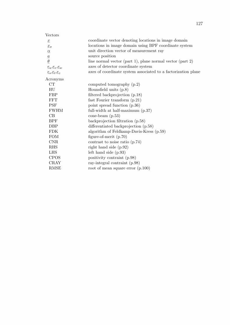
127
Vectorsx coordinate vector denoting locations in image domainxπ locations in image domain using BPF coordinate systemα unit direction vector of measurement raya source positionθ line normal vector (part 1), plane normal vector (part 2)eu,ev,ew axes of detector coordinate systemes,et,ez axes of coordinate system associated to a factorization plane
AcronymsCT computed tomography (p.2)HU Hounsfield units (p.8)FBP filtered backprojection (p.18)FFT fast Fourier transform (p.21)PSF point spread function (p.36)FWHM full-width at half-maximum (p.37)CB cone-beam (p.53)BPF backprojection filtration (p.58)DBP differentiated backprojection (p.58)FDK algorithm of Feldkamp-Davis-Kress (p.59)FOM figure-of-merit (p.70)CNR contrast to noise ratio (p.74)RHS right hand side (p.92)LHS left hand side (p.93)CPOS positivity contraint (p.98)CRAY ray-integral contraint (p.98)RMSE root of mean square error (p.100)

128 Chapter 8. Conclusions and Outlook
List of Figures
1.1 The principle of computed tomography . . . . . . . . . . . . . . . . . . . . . 21.2 X-ray CT systems used in medical imaging . . . . . . . . . . . . . . . . . . 3
2.1 Illustration of one exemplary measurement ray . . . . . . . . . . . . . . . . 8
3.1 The 2D parallel-beam geometry . . . . . . . . . . . . . . . . . . . . . . . . . 123.2 Illustration of the 2D Radon transform operator . . . . . . . . . . . . . . . 133.3 The 2D Shepp-Logan phantom . . . . . . . . . . . . . . . . . . . . . . . . . 153.4 Effects of the backprojection operator . . . . . . . . . . . . . . . . . . . . . 163.5 Data redundancies in 2D parallel-beam data . . . . . . . . . . . . . . . . . . 193.6 The ramp filter with rectangular band-limitation . . . . . . . . . . . . . . . 203.7 Results of the numerical 2D parallel-beam reconstruction algorithm . . . . . 213.8 The 2D fan-beam geometry . . . . . . . . . . . . . . . . . . . . . . . . . . . 223.9 Fan-beam data of the Shepp-Logan phantom . . . . . . . . . . . . . . . . . 243.10 Parker weighting function . . . . . . . . . . . . . . . . . . . . . . . . . . . . 263.11 Illustration of the numerical 2D fan-beam reconstruction algorithm . . . . . 27
4.1 Geometric illustration of redundantly measured lines . . . . . . . . . . . . . 334.2 Sampling schemes for the bandlimited Hilbert kernel . . . . . . . . . . . . . 354.3 Point spread function reconstructions . . . . . . . . . . . . . . . . . . . . . . 364.4 Plots of the FWHM . . . . . . . . . . . . . . . . . . . . . . . . . . . . . . . 364.5 Reconstructions of the FORBILD thorax phantom . . . . . . . . . . . . . . 394.6 Standard-deviation images . . . . . . . . . . . . . . . . . . . . . . . . . . . . 404.7 Comparison of image noise . . . . . . . . . . . . . . . . . . . . . . . . . . . 404.8 Pseudo-code of the backprojection operation . . . . . . . . . . . . . . . . . . 414.9 Fan-beam data of the physical QRM phantom . . . . . . . . . . . . . . . . . 424.10 Reconstruction of the QRM phantom . . . . . . . . . . . . . . . . . . . . . . 434.11 Standard-deviation in the real data reconstructions . . . . . . . . . . . . . . 444.12 Noise study, real fan-beam data . . . . . . . . . . . . . . . . . . . . . . . . . 454.13 Spatial resolution study, real fan-beam data . . . . . . . . . . . . . . . . . . 46
5.1 The 3D Radon plane . . . . . . . . . . . . . . . . . . . . . . . . . . . . . . . 505.2 3D Radon data of the 3D Shepp-Logan Phantom . . . . . . . . . . . . . . . 515.3 Intermediate 3D Radon values associated to circular CB data . . . . . . . . 555.4 Intermediate 3D Radon values associated to a partial circular scan . . . . . 56
6.1 Short-scan CB acquisition geometry . . . . . . . . . . . . . . . . . . . . . . 606.2 Geometric description of the planar 2D detector . . . . . . . . . . . . . . . 626.3 Coordinate system used by the BPF methods . . . . . . . . . . . . . . . . . 67
129
130 List of Figures
6.4 Slice through the CB performance phantom . . . . . . . . . . . . . . . . . . 716.5 Illustration of the profile matching approach . . . . . . . . . . . . . . . . . . 726.6 Spatial resolution in x− y and z in the plane of the scan . . . . . . . . . . . 746.7 Illustration of regions SA and SB for a phantom insert. . . . . . . . . . . . . 756.8 CNR measurements . . . . . . . . . . . . . . . . . . . . . . . . . . . . . . . 766.9 Estimates of the CNR inside the plane of the scan . . . . . . . . . . . . . . 766.10 Interdependence between total resolution and CNR . . . . . . . . . . . . . . 776.11 Dependence of the CNR on the z-coordinate . . . . . . . . . . . . . . . . . . 786.12 CB artifact measurements with the FORBILD head phantom . . . . . . . . 806.13 True density values of the investigated phantoms . . . . . . . . . . . . . . . 816.14 CB artifacts in the head phantom reconstruction . . . . . . . . . . . . . . . 826.15 Dependency of CB artifacts on the scan-range of the short-scan . . . . . . . 836.16 CB artifact evaluation using the disk phantom . . . . . . . . . . . . . . . . 846.17 Truncated and non-truncated CB data of the thorax phantom . . . . . . . . 866.18 Evaluation of axial truncation artifacts . . . . . . . . . . . . . . . . . . . . . 87
7.1 Geometric entities related to the plane of interest . . . . . . . . . . . . . . . 907.2 Relation between the intermediate function and object density . . . . . . . 927.3 CB data truncation and its impact on the planar reconstruction . . . . . . . 947.4 Sampling scheme on a plane of interest . . . . . . . . . . . . . . . . . . . . . 977.5 Singular values of an example system matrix . . . . . . . . . . . . . . . . . 987.6 Impact of parameter alpha on image quality . . . . . . . . . . . . . . . . . . 1017.7 Reconstruction of the disk phantom . . . . . . . . . . . . . . . . . . . . . . 1027.8 Impact of parameter sigma on image quality . . . . . . . . . . . . . . . . . . 1037.9 Spatial resolution evaluation for the factorization method . . . . . . . . . . 1047.10 Noise evaluation for the factorization method . . . . . . . . . . . . . . . . . 1057.11 CB artifact evaluation using the FORBILD head phantom . . . . . . . . . . 1067.12 Quantitative CB artifact study for the factorization method . . . . . . . . . 1077.13 Reconstruction results of the FORBILD head phantom . . . . . . . . . . . . 1087.14 A vertical slice through the FORBILD head phantom reconstruction . . . . 1097.15 Disk phantom reconstruction . . . . . . . . . . . . . . . . . . . . . . . . . . 1097.16 Axial truncation artifacts in the factorization method . . . . . . . . . . . . 1107.17 Reconstruction from the real C-arm data set A . . . . . . . . . . . . . . . . 1137.18 Reconstruction from the real C-arm data set B . . . . . . . . . . . . . . . . 115

List of Tables
4.1 Fan-beam geometry parameters . . . . . . . . . . . . . . . . . . . . . . . . . 344.2 Execution times for the investigated algorithms . . . . . . . . . . . . . . . . 42
6.1 C-arm geometry parameters . . . . . . . . . . . . . . . . . . . . . . . . . . . 70
131

132 List of Tables
Bibliography
[1] Antropomorphic Cardio CT Phantom, Quality Assurance in Radiology and Medicine(QRM) GmbH, Moehrendorf, Germany.
[2] AXIOM Artis dBA: Biplane C-arm system with flat detector for angiography, SiemensAG, Medical Solutions.
[3] Description of the FORBILD phantoms, online at: http://www.imp.uni-erlangen.de/forbild/english/results/index.htm.
[4] F. Noo. Lecture notes in Computed Tomography, Utah Center for Advanced ImagingResearch (UCAIR), University of Utah, USA.
[5] Performance in CT: SOMATOM Sensation, Datasheet for 64-slice Configuration,Siemens AG, Medical Solutions.
[6] There’s so much more to zee: Article from the customer magazine AXIOM Innova-tions, Nov. 2007, Siemens AG, Medical Solutions.
[7] I. Arai, H. Kudo, F. Noo, M. Defrise, and J. D. Pack. A new class of super-short-scan algorithms for fan-beam reconstruction. In IEEE Nuclear Science SymposiumConference Record, volume 4, pages 2296–2300, Puerto Rico, USA, 2005.
[8] A. Assmus. Early history of X rays. Beam Line periodicals, Standford University,Summer 95, pages 10–24, 1995.
[9] A. Bakushinsky and A. Goncharsky. Ill-Posed Problems: Theory and Applications(Mathematics and Its Applications). Springer-Verlag, Kluwer Academic Publishers(New York), 1994.
[10] G. Besson. CT image reconstruction from fan-parallel data. Med. Phys., 26(3):415–426, 1999.
[11] I. N. Bronstein and K. A. Semendjajew. Taschenbuch der Mathematik, 25. BGTeubner Verlagsgesellschaft und Verlag Nauka (Stuttgart Leipzig Moskau), 1991.
[12] T. M. Buzug. Einfuehrung in die Computertomographie. Springer (Berlin), 2004.
[13] G. H. Chen. An alternative derivation of Katsevich’s cone-beam reconstruction for-mula. Med. Phys., 30(12):3217–3226, 2003.
[14] G. H. Chen, R. Tokalkanahalli, T. Zhuang, B. E. Nett, and J. Hsieh. Developmentand evaluation of an exact fan-beam reconstruction algorithm using an equal weight-ing scheme via locally compensated filtered backprojection (LCFBP). Med. Phys.,33(2):475–481, 2006.
133
134 Bibliography
[15] Z. Chen, R. Ning, D. L. Conover, and Y. Yu. Quantitative assessment of cone-beamCT system by 3D point-spread function. In Proceedings of the SPIE, volume 5368,pages 574–585, San Diego, CA, USA, 2004.
[16] E. K. P. Chong and S. H. Zak. An Introduction to Optimization. John Wiley andSons, Inc., 1996.
[17] R. Clack and M. Defrise. Cone-beam reconstruction by the use of Radon transformintermediate functions. J. Opt. Soc. Am. A, 11(2):580–585, 1994.
[18] R. Clack and M. Defrise. Overview of reconstruction algorithms for exact cone-beamtomography. In Proc. SPIE, volume 2299, pages 230–241, San Diego, CA, USA, 1994.
[19] S. R. Deans. The Radon transform for higher dimensions. Phys. Med. Biol.,23(6):1173–1175, 1978.
[20] M. Defrise and R. Clack. A cone-beam reconstruction algorithm using shift-variantfiltering and cone-beam backprojection. IEEE Trans. Med. Imag., 13(1):186–195,1994.
[21] M. Defrise and G. T. Gullberg. Image reconstruction. Phys. Med. Biol., 51(13):139–154, 2006.
[22] M. Defrise, F. Noo, R. Clackdoyle, and H. Kudo. Enlargement of the region of accuratereconstruction in computed tomography from truncated data. In Proceedings Fully3D Meeting and HPIR Workshop, pages 46–50, Salt Lake City, UT, USA, 2005.
[23] F. Dennerlein, A. Katsevich, G. Lauritsch, and J. Hornegger. Exact and efficientcone-beam reconstruction algorithm for a short-scan circle combined with variouslines. In Proceedings of the SPIE, volume 5747, pages 388–399, San Diego, CA, USA,2005.
[24] F. Dennerlein, F. Noo, W. Haerer, J. Hornegger, and G. Lauritsch. Constriction ofcone-beam artifacts by the z-smart reconstruction method. In IEEE Nuclear ScienceSymposium Conference Record, volume 6, pages 4090–4096, Honolulu, Hawaii, USA,2007.
[25] F. Dennerlein, F. Noo, S. Hoppe, J. Hornegger, and G. Lauritsch. Cone-beam tomog-raphy with linearly distorted source trajectories. In IEEE Nuclear Science SymposiumConference Record, volume 4, pages 2311–2315, San Diego, USA, 2006.
[26] F. Dennerlein, F. Noo, J. Hornegger, and G. Lauritsch. Factorization of the recon-struction problem in circular cone-beam tomography and its use for stability analysis.In IEEE Nuclear Science Symposium Conference Record, volume 5, pages 2908–2912,San Diego, CA, USA, 2006.
[27] F. Dennerlein, F. Noo, G. Lauritsch, and J. Hornegger. Fan-beam filtered-backprojection reconstruction without backprojection weight. Phys. Med. Biol.,52(11):3227–3240, 2007.
[28] F. Dennerlein, F. Noo, H. Schoendube, J. Hornegger, and G. Lauritsch. Cone-beamreconstruction on a circular short-scan using the factorization approach. In Proceed-ings of the Fully3D, pages 346–349, Lindau, Germany, 2007.
Bibliography 135
[29] F. Dennerlein, F. Noo, H. Schoendube, J. Hornegger, and G. Lauritsch. A factoriza-tion approach for cone-beam reconstruction on a circular short-scan. IEEE Trans.Med. Imag., 27(7):887–896, 2008.
[30] K. Doi. Diagnostic imaging over the last 50 years: Research and development inmedical imaging science and technology. Phys. Med. Biol., 51(13):5–27, 2006.
[31] J. Eriksson. Problems and experiments in cone-beam tomography. Linkoeping studiesin science and technology (Linkoeping University), 1998.
[32] A. Faridani, R. Hass, and D. C. Solmon. Numerical and theoretical explorations inhelical and fan-beam tomography. J. Phys.: Conf. Ser., 124(1):ID 012024, 2008.
[33] L. A. Feldkamp, L. C. Davis, and J. W. Kress. Practical cone-beam algorithm. J.Opt. Soc. Am. A, 1(6):612–619, 1984.
[34] D. V. Finch. Cone-beam reconstruction with sources on a curve. SIAM J. Appl.Math., 45(4):665–673, 1985.
[35] R. Gordon, R. Bender, and G. T. Herman. Algebraic reconstruction techniques (ART)for three-dimensional electron microscopy and X-ray photography. Journal of Theo-retical Biology, 29(3):471–481, 1970.
[36] P. Grangeat. Mathematical framework of cone-beam 3D reconstruction via the firstderivative of the Radon transform. Lecture Notes in Mathematics, G. T. Herman, A.K. Louis, F. Natterer, Eds., 1497:66–97, 1991.
[37] M. Grass, T. Koehler, and R. Proksa. 3D cone-beam CT reconstruction for circulartrajectories. Phys. Med. Biol., 45(2):329–347, 2000.
[38] R. I. Hartley and A. Zisserman. Multiple View Geometry in Computer Vision. Cam-bridge University Press, 2004.
[39] G. T. Herman. Image Reconstruction from Projections - The Fundamentals of Com-puterized Tomography. Academic Press, 1980.
[40] S. Hoppe, F. Dennerlein, G. Lauritsch, J. Hornegger, and F. Noo. Cone-beam tomog-raphy from short-scan circle-plus-arc data measured on a C-arm system. In IEEENuclear Science Symposium Conference Record, 2006. IEEE, volume 5, pages 2873 –2877, San Diego, CA, USA, 2006.
[41] S. Hoppe, J. Hornegger, G. Lauritsch, F. Dennerlein, and F. Noo. Geometric calibra-tion of the circle-plus-arc trajectory. Phys. Med. Biol., 52(23):6943–6960, 2007.
[42] S. Hoppe, J. Hornegger, G. Lauritsch, F. Dennerlein, and F. Noo. Truncation cor-rection for non-horizontal filter lines. In Proceedings Fully 3D Meeting and HPIRWorkshop, volume 9, pages 209–212, Lindau, Germany, 2007.
[43] J. Hsieh and X. Tang. Conjugate backprojection approach for cone beam artifactreduction. In Proceedings of the SPIE, volume 6142, pages 758–764, San Diego, CA,USA, 2006.
[44] H. Hu. A new cone beam reconstruction algorithm for the circular orbit. In IEEENuclear Science Symposium Conference Record, volume 3, pages 1261–1265, 1994.
136 Bibliography
[45] A. N. Iusem. On the convergence properties of the projected gradient method forconvex optimization. Mat. apl. comput., 22(1):37–52, 2003.
[46] A. C. Kak and M. Slaney. Principles of Computerized Tomographic Imaging. IEEEPress, 1988.
[47] W. A. Kalender. Computed Tomography - Fundamentals, System Technology, ImageQuality, Applications, 2nd edition. Publicis Corporate Publishing (Erlangen), 2005.
[48] W. A. Kalender. X-ray computed tomography. Phys. Med. Biol., 51(13):29–43, 2006.
[49] A. Katsevich. Analysis of an exact inversion algorithm for spiral cone-beam CT.Phys. Med. Biol., 47(15):2583–2597, 2002.
[50] A. Katsevich. A general scheme for constructing inversion algorithms for cone beamCT. IEEE Trans. Med. Imag., 21:1305–1321, 2003.
[51] A. Katsevich. Image reconstruction for the circle and line trajectory. Phys. Med.Biol., 49(22):5059–5072, 2004.
[52] A. Katsevich. Image reconstruction for the circle-and-arc trajectory. Phys. Med.Biol., 50(10):2249–2265, 2005.
[53] A. Katsevich, K. Taguchi, and A. A. Zamyatin. Formulation of four Katsevich algo-rithms in native geometry. IEEE Trans. Med. Imag., 25(7):855–868, 2006.
[54] T. Kido, A. Kurata, H. Higashino, Y. Sugawara, H. Okayama, J. Higaki, H. Anno,K. Katada, S. Mori, S. Tanada, M. Endo, and T. Mochizuki. Cardiac imaging us-ing 256-detector row four-dimensional CT: preliminary clinical report. RadiationMedicine, 25(1):38–44, 2007.
[55] H. Kudo, M. Courdurier, F. Noo, and M. Defrise. Tiny a priori knowledge solves theinterior problem in computed tomography. Phys. Med. Biol., 53(9):2207–2231, 2008.
[56] H. Kudo, F. Noo, M. Defrise, and R. Clackdoyle. New super-short-scan algorithmfor fan-beam and cone-beam reconstruction. In IEEE Nuclear Science SymposiumConference Record, volume 2, pages 902–906, Norfolk, VA, USA, 2002.
[57] H. Kudo and T. Saito. Derivation and implementation of a cone-beam reconstructionalgorithm for non-planar orbits. IEEE Trans. Med. Imag., 13(1):196–211, 1994.
[58] R. B. Marr, C. N. Chen, and P. C. Lauterbur. On two approaches to 3D reconstructionin NMR zeugmatography. Proc. mathematical aspects of computerized tomography,Lecture notes in medical informatics, 8:225–240, 1981.
[59] T. Moore and E. Rohm. Application Protocol Book for AXIOM Artis 3D applica-tions. Siemens AG, Medical Solutions, Angiography, Fluoroscopic and RadiographicSystems (Forchheim), 2007.
[60] J. Moret. 3D rotational angiography: Clinical value in endovascular treatment. Med-ica Mundi, 42(3):8–14, 1998.
[61] O. Nakamura, S. Kawata, and S. Minami. Optical microscope tomography. II. Non-negative constraint by a gradient-projection method. J. Opt. Soc. Am. A, 5(4):554–561, 1988.
Bibliography 137
[62] F. Natterer. The Mathematics of Computerized Tomography. John Wiley, Sons Inc,1986.
[63] F. Natterer and F. Wuebbeling. Mathematical Methods in Image Reconstruction.Society for Industrial and Applied Mathematics (SIAM), 2001.
[64] B. E. Nett, T. L. Zhuang, S. Leng, and G. H. Chen. Arc-based cone-beam recon-struction algorithm using an equal weighting scheme. J. of X-ray Sci. and Tech.,15(1):19–48, 2007.
[65] F. Noo, R. Clackdoyle, and J. D. Pack. A two-step hilbert transform method for 2Dimage reconstruction. Phys. Med. Biol., 49(17):3903–3923, 2004.
[66] F. Noo, M. Defrise, R. Clackdoyle, and H. Kudo. Image reconstruction from fan-beamprojections on less than a short scan. Phys. Med. Biol., 47(14):2525–2546, 2002.
[67] F. Noo and D. J. Heuscher. Image reconstruction from cone-beam data on a circularshort-scan. In Proceedings of the SPIE, volume 4684, pages 50–59, San Diego, CA,USA, 2002.
[68] F. Noo, S. Hoppe, F. Dennerlein, G. Lauritsch, and J. Hornegger. A new scheme forview-dependent data differentiation in fan-beam and cone-beam computed tomogra-phy. Phys. Med. Biol., 52(17):5393–5414, 2007.
[69] F. Noo, J. D. Pack, and D. Heuscher. Exact helical reconstruction using nativecone-beam geometries. Phys. Med. Biol., 48(23):3787–3818, 2003.
[70] B. B. Ohnesorge, T. G. Flohr, C. R Becker, A. Knez, and M. F. Reiser. Multi-sliceand Dual-source CT in Cardiac Imaging. Springer (Berlin), 2006.
[71] A. Oppelt. Imaging Systems for Medical Diagnostics. Publicis Corporate Publishing(Erlangen), 2005.
[72] J. D. Pack, F. Noo, and R. Clackdoyle. Cone-beam reconstruction using the backpro-jection of locally filtered projections. IEEE Trans. Med. Imag., 24(1):70–85, 2005.
[73] X. Pan. Optimal noise control in and fast reconstruction of fan-beam computedtomography image. Med. Phys., 26(5):689–697, 1999.
[74] X. Pan and L. Yu. Image reconstruction with shift-variant filtration and its impli-cation for noise and resolution properties in fan-beam computed tomography. Med.Phys., 30(4):590–600, 2003.
[75] D. L. Parker. Optimal short scan convolution reconstruction for fan-beam CT. Med.Phys., 9(2):254–257, 1982.
[76] J. Radon. Ueber die Bestimmung von Funktionen durch ihre Integralwerte laengsgewisser Mannigfaltigkeit. Berichte Saechs. Akad. Wiss., Math. Phys. Kl, 69:262 –277, 1917.
[77] W. C. Roentgen. Ueber eine neue Art von Strahlen. Annalen der Physik, 300(1):12–17, 1898.
138 Bibliography
[78] S. Schaller, T. Flohr, and P. Steffen. An efficient Fourier method for 3-D Radoninversion in exact cone-beam CT reconstruction. IEEE Trans. Med. Imag., 17(2):244–250, 1998.
[79] M. D. Silver. A method for including redundant data in computed tomography. Med.Phys., 27:773–774, 2000.
[80] B. D. Smith. Image reconstruction from cone-beam projections: necessary and suffi-cient conditions and reconstruction methods. IEEE Trans. Med. Imag., 4(1):14–25,1985.
[81] B. D. Smith. Cone-beam tomography: Recent advances and a tutorial review. Opt.Eng., 29(5):524–534, 1990.
[82] H. Turbell. Cone-Beam Reconstruction Using Filtered Backprojection. Linkoepingstudies in science and technology (Linkoeping University), 2001.
[83] H. K. Tuy. An inversion formula for cone-beam reconstruction. SIAM J. Appl. Math.,43(3):546–552, 1983.
[84] S. Valton, F. Peyrin, and D. Sappey-Marinier. Analysis of cone-beam artifacts inoff-centered circular CT for four reconstruction methods. Int. J. Biomed. Imag.,2006.
[85] R. VanTiggelen. In search for the third dimension: From radiostereoscopy to three-dimensional imaging. JBR-BTR, 85:266–270, 2002.
[86] G. Wang, Y. Liu, T. H. Lin, and P. C. Cheng. Half-scan cone-beam X-ray microto-mography formula. Scanning, 16(4):216–220, 1994.
[87] G. Wang, S. Zhao, and P Cheng. Exact and approximate cone-beam X-ray microto-mography. Modern Microscopies (I) - Instrumentation and Image Processing, WorldScientific, Singapore, pages 1–14, 1998.
[88] K. Wiesent, K. Barth, N. Navab, P. Durlak, T. Brunner, O. Schuetz, and W. Seissler.Enhanced 3-D-reconstruction algorithm for C-arm systems suitable for interventionalprocedures. IEEE Trans. Med. Imag., 19(5):391–403, 2000.
[89] A. Wunderlich and F. Noo. Image covariance and lesion detectability in direct fan-beam X-ray computed tomography. Phys. Med. Biol., 53(10):2471–2493, 2008.
[90] D. Xia, L. Yu, E. Y. Sidky, Y. Zou, N. Zuo, and X. Pan. Noise properties of chord-image reconstruction. IEEE Trans. Med. Imag., 26(10):1328–1344, 2007.
[91] Y. Yao, L. Rosasco, and A. Caponnetto. On early stopping in gradient descentlearning. Constructive Approximation, 26(2):289–315, 2007.
[92] H. Yu and G. Wang. Feldkamp-type VOI reconstruction from super-short-scan cone-beam data. Med. Phys., 31(6):1357–1362, 2004.
[93] L. Yu, Y. Zou, E. Y. Sidky, C. A. Pelizzari, P. Munro, and X. Pan. Region of interestreconstruction from truncated data in circular cone-beam CT. IEEE Trans. Med.Imag., 25(7):869–881, 2006.
Bibliography 139
[94] A. A. Zamyatin, K. Taguchi, and M. D. Silver. Practical hybrid convolution algorithmfor helical CT reconstruction. IEEE Trans. Nucl. Sci., 53(1):167–174, 2006.
[95] M. Zellerhoff, B. Scholz, E. P. Ruehrnschopf, and T. Brunner. Low contrast 3D-reconstruction from C-arm data. In Proceedings of the SPIE, volume 5745, pages646–655, San Diego, CA, USA, 2005.
[96] G. L. Zeng. Nonuniform noise propagation by using the ramp filter in fan-beamcomputed tomography. IEEE Trans. Med. Imag., 23(6):690 – 695, 2004.
[97] K. Zeng, Z. Chen, L. Zhang, and G. Wang. A half-scan error reduction based algo-rithm for cone-beam CT. J. of X-ray Sci. and Tech., 12:73–82, 2004.
[98] S. Zhao, H. Yu, and G. Wang. A unified framework for exact cone-beam reconstructionformulas. Med. Phys., 32(6):1712–1721, 2005.
[99] T. Zhuang, S. Leng S, B. E. Nett, and G. H. Chen. Fan-beam and cone-beam imagereconstruction via filtering the backprojection image of differentiated projection data.Phys. Med. Biol., 49(24):5489–5503, 2004.
[100] Y. Zou and X. Pan. Exact image reconstruction on pi-lines from minimum data inhelical cone-beam CT. Phys. Med. Biol., 49(6):941–59, 2004.