image restoration using adaptive nonlinear techniques
TRANSCRIPT

Republic of Iraq
Ministry of Higher Education & Scientific Research
Al-Nahrain University
College of Science
Image Restoration Using Adaptive Nonlinear Techniques
A Thesis
Submitted to the College of Science of Al-Nahrain University as a Partial Fulfillment of the Requirements for the Degree of Master of
Science in Physics
By
Mohammed Khudier Kadhom
(B.Sc. 2005)
Supervised by
Professor Dr. Ayad A. Al-Ani
Assistant Professor Dr. Salah A. Saleh
Rabi' Thani. April
1429 2008

الرحيم الرحمن الله بسم
والمؤمنون ورسوله عملكم الله فسيرى اعملوا وقل بما فينبئكم والشهادة الغيب عالم إلى وستردون
تعملون كنتم
صدق الله العظيم
)١٠٥:التوبة(

List of Contents
Certification
Acknowledgment
Abstract
page
1 3 6 6
Chapter One: General Introduction
1.1 Introduction
1.2 Historical Survey
1.3 Aim of the Thesis
1.4 Thesis Layouts
8
9
10
11
11
11
12
13
14
18
18
19
19
20
Chapter Two: Image Model and Image Manipulation
2.1 Introduction
2.2 Image Formation
2.2.1 Blur Model (point spread function)
Space - Invariant Point Spread Function (SIPSF)
Space -Variant Point Spread Function (SVPSF)
a. Atmospheric turbulence blur (Gaussian blur)
b. Motion Blur
c. Uniform Out Of Focus Blur
2.3 Noise Model
a. Additive Noise
b. Multiplicative Noise
2.4 Image Restoration
2.4.1 Image Restoration Algorithms
I. Frequency Domain Filters

20
21
23
24
28
32
33
33
35
74
77
77
78
1. Inverse Filter
2. Wiener Filter
3. Constrained Least-Squares Filter
II. Iterative image restoration algorithms
3.5 Image Quality
Chapter Three: Results and Discussion
3.1 Introduction
3.2 Practical Part
Image Restoration Algorithm
3.3 Results
3.4 Results discussion
Chapter Four: Conclusions and Future Work
4.1 Conclusions
4.2 Suggest For Future Work
References


Acknowledgments
Thanks to our GOD the most merciful and gracious for
enabling me to complete this thesis.
I would like to express my sincere thanks and deep
gratitude to my supervisors Professor Dr. Ayad A. Al-Ani and
Assistant Professor Dr. Salah A. Saleh for supervising the
present work and for their support, encouragement and
suggestions throughout the work.
Special thanks and deep affection to my family, and my
wife for their love, help, and supports through the years.
Finally, I would like to extend my thanks and gratitude to
all who had ever assisted me during the period of this research.
`É{tÅÅxw ^{âw|xÜ

Abstract
Image restoration is the process of finding an approximation to the
degradation process and find appropriate inverse process to estimate the
original image.
An iterative restoration technique(Tikhonov method) was adapted.
The adapted filter was designed for restoring RGB satellite images that
are blurred with space-invariant point spread function, Gaussian
function, and corrupted with additive noise, and salt & pepper noise.
Different degradation parameters, i.e. different signal to noise ratio were
considered and different noise density.
The results using an adaptive filter were compared,
quantitatively, with different types of conventional restoration techniques,
(such as inverse filter, Least-Squares filter (Wiener Filter), and
Constrained Least-Squares filter) using Mean Square Error (MSE).
Results show that The Mean Square Error of the restored images
decreases with increasing the number of iteration until the result
convergence. Also the ratio of the MSE of the degraded image to the
restored image will increase with decreasing SNR for Gaussian noise,
and with increasing noise density for salt and pepper noise respectively,
then Results show this method has better performance for restoring the
degraded images, especially for low signal to noise ratio, and for high
noise density.

Chapter One General Introduction
0
CHAPTER ONE

Chapter One General Introduction
1
General Introduction 1.1
The term digital has become part of our daily lives. It derives from
Latin digitus, finger, and has since then quite understandably come to
mean 'numerical' or 'number-related'. The word is known from constructs
such as 'digital clock' (a clock showing time as numbers or digits); even
'digital sound' is a well-known concept today [1].
The field of digital image processing has a quite long history in
astronomy that began in the 1950's with the space program. The first
images of Moon (mainly of the opposite side), at that time of
unimaginable resolution. However, the images were obtained under big
technical difficulties such as vibrations, motion due spinning, etc. The
need to retrieve as much information as possible from such degraded
images was the aim of the early efforts to adapt the one-dimensional
signal processing algorithms to images, creating a new field that is today
known as "Digital Image Processing" [2].
The techniques of image reconstruction and restoration have been
a "must" in all scientific disciplines involving projections or
interferometer data. However, for a long time image processing was
considered as a luxury in other fields such as optical astronomy. It also
applied to image coming from space [3].
The term digital image processing generally refers to processing of
a two-dimensional picture by a digital computer [4].
Interest in digital image processing methods stems from two
principal application areas: improvement of pictorial information for
human interpretation. And processing of scene data for autonomous
.machine perception [5].
Digital image processing has a broad spectrum of applications,
such as remote sensing via satellites and other spacecrafts, image
transmission and storage for business applications, medical processing,

Chapter One General Introduction
2
radar, sonar, and acoustic image processing, robotics, and automated
inspection of industrial parts [4].
Typical problems in machine perception that routinely employ
image processing techniques are automatic character recognition,
industrial robots for product assembly and inspection, military
recognizance, automatic processing of fingerprints, screening of x-rays
and blood samples, and machine processing of aerial and satellite imager
for weather prediction and crop assessment [5].
Image restoration is the process of taking an image with some
known, or estimated degradation, the restoring it to its original
appearance, Image restoration often used in the field of photography or
publishing where an image was somehow degraded but needs to be
improved before it can be printed. For this type of application, know are
needed to something about the degradation process in order to develop
model for the distortion. When a model for the degradation process has,
the inverse process can be applied to the image to restore it to its original
form [6].
There are no techniques so far, that can produce a perfect
restoration or that can be recommend for use in each and every case of
degradation. In order to choose or to design a method of image
restoration it is necessary and very important to characterize the
degradation effect and also some prior information about the degraded
image [7].

Chapter One General Introduction
3
1.2 Historical Survey
Detailed discussion of the earlier developments in restoration
techniques can be found in Sondi, Andrews, Hunt, Rosenfeld and Kak,
Bates et. al., Gonzalz and Wintz , Sezan & Tekalp. Unfortunately, the
book by Andrews and Hunt, published in 1977 is the only available book
specialized in the field of image restoration [8].
In fact, a variety of digital techniques has been proposed and
developed for the enhancement or restoration considering the recovering
of original images from degraded images. However, it can be seen from the
published literature that a number of image restoration techniques have
been derived from linear filtering [9]. One basic approach for stochastic
methods is to use the Wiener filter in the frequency domain and then linear
restoration filter in the spatial domain [10].
In the past few years there has been great interest in the development
of recursive filtering techniques for time domain signals. These
techniques have been recently applied to image restoration [8] with the
hope of alleviating the high computational burden and obtaining optimal
restoration [10].
In 1987, Denise, and Howard [11] were developed color image
restoration, taking into account the correlation between color
components.
In1999, Geert and Lucas [12] were studied the essential difference
of non-linear image restoration algorithms with linear image restoration
filter is their capability to restrict the restoration result to non-negative
intensities. The Iterative Constrained Tikhnov-Miller algorithm (ICTM)
algorithms. They are showed that this dramatically deteriorate the
performance of the non-linear restoration algorithms. And they are
proposing a novel method to estimate the background based on the
dependency of non-linear restoration algorithms on the background.

Chapter One General Introduction
4
In 2000, Geert and Lucas [13] were studied on the influence of the
regularization parameter and the first estimate on the performance of
iterative image restoration algorithms. They were discussed regularization
parameter estimation methods that have been developed for the linear
Tikhonov – Miller filter to restore images distorted by additive Gaussian
noise; they found that most algorithms converged for most choices.
In 2003, Hao and his college [14] were presented a new teqnique
for acceleration of iterative image restoration algorithms, unlike other fast
algorithms which tend to accelerate the rate of convergence of iterative
procedure.
In 2003, Sang and his college [15] were introduced the
regularization method to suppress over-amplification. However, the
regularization causes the reblurring problem and does not eliminate
ringing artifacts effectively. A directional regularization approach is
proposed to reduce the reblurring problem and the ringing artifacts in
iterative image restoration.
In 2004, Stuart at el. [16] were developed a novel, perceptually
inspired image restoration method which takes human perception
knowledge into consideration to reverse the effect blur; they have been
show that the new restoration algorithm visually restores images as well
as the previously presented LVMSE-based algorithm.
In 2005,Yuk and Yik[17] were studied the restoration of color-
quantized images, they are proposed a restoration algorithm for restoring
color-quantized images, simulation results show that it can improve the
quality of a color –quantized image remarkably in terms of both SNR and
CIELAB color difference metric.
In 2006,Feng at el. [18] were presented a new iterative
regularization algorithm. Before restoration, they have been divided the
pixels of the blurred and noisy image into two types of regions: flat

Chapter One General Introduction
5
region and edge region (edge and the regions near edge), and they are
showed that algorithm is effective and the edge details are well preserved
during the restoration process.
In 2006, Paola at el. [19] were studied in many image restoration
applications the nonnegative of the computed solution is required.
General regularization methods, such as iterative semi convergent
methods, seldom compute nonnegative solutions even when the data are
nonnegative. Some methods can be modified in order to enforce the
nonnegative constraint.
In 2006, Ayad A. Al-ani [20] was adapted in many image
restorations an iterative Wiener filter. To estimate the power spectral
density of the original image from degraded image using an iterative
method. The adapted filter was designed for restoring astronomical
images that are blurred with space-invariant point spread function and
corrupted with additive noise .the result using an adaptive filter were
compared, quantitatively, using mean square error (MSE).His result
shows that this method has better performance for restoring the degraded
images, especially for high signal to noise ratio.
In 2007,Tony and his college [21] were discussed studied many
variant ional models for image denoising restoration are formulated in
primal variables that are directly linked to the solution to be restored ,they
are proposed a linearized primal dual iterative method as an alternative
stand-alone approach to solve the dual formulation without
regularization. Numerical results are presented to show that the proposed
methods are much faster than the Chambolle method.
In 2007, Wenyi and his college [22] were discussed the task of
deblurring, a form of image restoration, is to recover an image form its
blurred version. Whereas most existing methods assume a small amount
of additive noise, image restoration under significant additive noise

Chapter One General Introduction
6
remains an interesting research problem. They are described two
techniques to improve the noise handling characteristics of a recently
proposed variational framework for semi-blind image deblurring that is
based on joint segmentation and deblurring. One technique uses a
structure tensor as a robust edge- indicating function. The other uses
nonlocal image averaging to suppress noise. They are reported promising
results with these techniques for the case of a known kernel.
1.3 Aim of the thesis
The aim of this thesis is to restore a degraded image, which
blurred by Gaussian function and corrupted by an additive white noise,
and salt and pepper noise using non linear method.
The adaptive technique is solved by estimating the power spectral
density of the original image" object" from the degraded image. The
adaptive technique (Tikhonov method) is compared with different types
of conventional restoration techniques (Inverse filter, Least-Square filter
(Weiner filter), constrained Least-Square filter (Regular filter)).
The aim of comparative study shows is one method better than
other.
1.4 Thesis Layout
This thesis is organized as follows:
Chapter one, presents a general introduction of image
processing.
Chapter two, deals with general background on the image
formation, and described the most important methods and filters
for image restoration and the parameters that effect the image
quality and the most important image quality function.

Chapter One General Introduction
7
Chapter three, describes the computer simulation models which
restore image by using (inverse filter, least Least-Squares Filter
(wiener Filter), and Constrained Least-Squares Filter (Regular
Filter, Tikhonov filter).
Chapter four contains the conclusions of this work and
suggestion for future work.

Image Formation and Image Manipulation Chapter Two
7
CHAPTER TWO

Image Formation and Image Manipulation Chapter Two
8
Introduction1.2
When light is reflected by emitted from an object, it travels to the
image plane through a medium which is not always homogenous. the
inhomogeneous of the medium produces some degree of distortion. The
source of distortion will be illustrated later in this chapter. This source
includes the blur and noise function. The blur function has two types
these are space variant and space invariant. The motion blur which is one
of blur function that is resulting from a motion of imaging system or the
object through the imaging period , atmospheric turbulence blur is
another type of blur model, aberration is another type of blur model, and
uniform out-of-focus is another type of blur model.
The ultimate goal of restoration techniques, however, is to improve
a given image in some sense. It is therefore, an attempt to reconstruct or
recover an image that has been degraded, using some a prior knowledge
of the degradation phenomenon [5].
Generally, image formation processes can be described with a
small number of equivalent physical concepts and an associated set of
equation. There are many algorithms developed to overcome the problem
of image restoration; e.g. linear and nonlinear, iterative and non-iterative,
recursive and non- recursive, generalized algorithms and specialized
algorithms. Some of these are applied in frequency domain while others
in spatial domain.
Image quality is the another subject in this chapter. Image quality
gives a criterion to show the degree of distortion between the reference
images and the degraded one of the same scene [3].

Image Formation and Image Manipulation Chapter Two
9
2.2 Image Formation
The term image simply, refers to a two-dimensional light intensity
function "g(x,y)" , where x and y denote spatial coordinates and the value
of g at any point (x,y) is proportional to the brightness (or gray level) of
the image at that point [5].
light is a form of energy, must be nonzero and finite; i.e. [ 5]:
0 < g(x,y) < ∞ (2-1)
The basic nature of g(x,y) may be characterized by two components [6]:
1 - The amount of source light incident on the scene being viewed.
2- The amount of light reflected by the objects in the scene.
Appropriately, they are called the illumination and reflectance
components, and are denoted by i(x,y) and r(x,y), respectively. The
function i(x,y) and r(x,y)combine as product to form g(x,y) [ 5]:
g(x,y)= i(x,y) r(x,y) (2-2)
where
0 < i(x,y) < ∞ (2-3)
and
0 < r(x,y) < 1 (2-4)
Equation (2-4) indicates that reflectance is bounded by 0(total
absorption) and 1 (total reflectance). The nature of i(x,y) is determined by
the light source, and r(x,y) is determined by the characteristics of the
object in a scene [6].
The degradation process model consists of two parts, the
degradation function and the noise function. The general model in the
spatial domain follows [6]:

Image Formation and Image Manipulation Chapter Two
10
(2-5)),(),(),(),( yxnyxfyxhyxg
where
denotes the convolution process
g(x,y) degraded image
h(x,y) degradation function, which is called point spread function (psf).
f(x,y) original image
n(x,y) additive noise function.
The Fourier Transform of eq. (2-5) is given by:
G(u, v) = H(u, v)F(u, v) + N(u, v) (2-6)
G(u,v) = Fourier transform of the degraded image.
H(u,v) = Fourier transform of the degraded function.
F(u,v) = Fourier transform of the original image.
N(u,v) = Fourier transform of the additive noise function.
H(u,v) is called the forward transfer function of the process. The
inverse transform of the system transfer function, is called the impulse
response in the terminology of linear system theory. H(u,v) is called optical
transfer function, and its magnitude is called the Modulation Transfer
Function [5].
2.2 .1 Blur Model point spread function
It represents the most operative image degradation. It determines the
energy distribution in the image plane due to point source located on the
object plane [ 3].
Blur model can categorized into two types [ 3]:
1-Space-Invariant Point Spread Function (SIPSF).
2-Space-Variant Point Spread Function (SVPSF).

Image Formation and Image Manipulation Chapter Two
11
1. Space-Invariant Point Spread Function (SIPSF)
The point source explores the object plane, the point spread
function changes only the position of the input but merely changes the
location of the output with keeping the same function, This characteristic
appears in the linear system. For example, the most optical telescope and
microscope.
Thus the final image can be represented by a convolution process with
ideal image f (x0, y0):
),(),()0
,0
(),( 0000 yxndydxyyxxhyxfyxg
(2-7)
Where ( x a , y 0 ) and (x,y) represent the coordinates of the object and
image form respectively[9].
2. Space-Variant Point Spread Function (SVPSF).
This type changes shape as well as position, i.e. the point spread
function depends on the location of the object ,this property associated
with nonlinear system [3].
a. Atmospheric turbulence blur
Atmospheric turbulence is severe limitation in Astronomy, remote
sensing and aerial imaging as used for example weather predictions.
Though the blur introduced by atmospheric turbulence depends on a
variety of factors (such as temperature, wind speed, exposure time), for
long term exposures the PSF can reasonably well be described by a
Gaussian function[23]:

Image Formation and Image Manipulation Chapter Two
12
2
22
2exp),,(
yx
Cyxh (2-8)
Here σ determines the severity of the blur. C is constant depends on
the type of turbulence which is usually found experimentally [24].
Figure(2-1) shows Gaussian blur in the Fourier domain:
Figure(2-1) Gaussian blur in the Fourier domain [23].
b. Motion Blur
Many types of motion blur can be distinguished, all of which are
due to relative motion between the recording device and the scene. This
can be in the form of a translation, a rotation, a sudden change of scale,
or some combinations of these. Here only the important case of a global
translation will be considered[23].
),( vuH

Image Formation and Image Manipulation Chapter Two
13
When the object translates at a constant velocity V under an angle
of φ radians with the horizontal axis during the exposure interval [ 0, T ],
then blurring function is given by [23]:
0
1),,,( LLyxh
The discrete version of eq. (2-9) is not easily captured in a closed form
expression in general. For the special case that =0, an appropriate
approximation eq. (2-9) is given by [23]:
0
2
121
2
1
1
),,,(L
LL
L
Lyxh
c. Uniform Out-Of-Focus Blur
When a camera images a 3-D scene onto a 2-D imaging plane,
some parts of the scene are in focus while other parts are not. If the
aperture of the camera is circular, the image of any point source is a
small disk, known as the Circle Of Confusion (COC). The degree of
defocus (diameter of the COC) depends on the focal length , the aperture
number of the lens, and the distance between camera and object. An
accurate model not only describes the diameter of the COC, but also the
intensity distribution within the COC. The spatially continuous PSF of
this uniform out-of-focus blur with radius R is given by[23]:
(2- 9) tan2
22 y
xLyxif
elsewhere
(2-10)
2
1,0 21
Lxx if
2
1,0 21
Lxxif
elsewhere

Image Formation and Image Manipulation Chapter Two
14
0
1),,( 2RRyxh
Figure(2-2) shows PSF in the Fourier domain of uniform out of focus
Blur:
Figure(2-2):PSF in the Fourier domain
(Uniform Out-Of-Focus Blur) [23].
2.3 Noise Model
Noise is any undesired information that contaminates an image [6 ].
Or, they are random background events which have to be dealt with in
every system processing real signals. They are not part of the ideal signal
and may be caused by a wide range of sources, e.g. variations in the
detector sensitivity, environmental variations, the discrete nature of
radiation, transmission or quantization errors, etc [ 4].
),( vuH
if 222 Ryx (2-11)
elsewhere

Image Formation and Image Manipulation Chapter Two
15
The noise can be modeled with either a Gaussian (normal),
uniform, or salt-and-pepper (impulse) distribution. The shape of the
distribution of these noise types as a function of gray level can be
modeled as a histogram.
Gaussian noise distribution which can be analytically described by [6]:
2
2
2)(
)(22
1
mg
gP e
(2-12)
where:
g= gray level
m= mean (average) 2 = variance of the noise.
The uniform distribution which is given by [6]:
0
1)( abgP For a ≤ g ≤ b (2-13)
where
2
bamean
12
)(var
2abiance
With the uniform distribution, the gray level values of the noise are
evenly distributed across a specific range [6].
The salt-and-pepper distribution is given by:
elsewhere
B
AgP pepperandsalt)(
For g=a ("pepper") (2-14)
For g=b ("salt")

Image Formation and Image Manipulation Chapter Two
16
In the salt-and-pepper noise model there are only two possible
values,a and b, and the probability of each is typically less than 0.1-with
number greater than this,. For 8-bit image, the typical value for pepper
noise is 0 and for salt is 255[6].
The Gaussian model is most often used to model natural noise
processes, such as those occurring from electronic noise in the image
acquisition system. The salt-and-pepper type noise is typical caused by
malfunctioning pixel elements in the camera sensor, faulty memory
locations, or timing error in the digitization process. Uniform is useful
because it can be used to general any other type of noise distribution and is
often used to degrade image for the evaluation of image restoration
algorithms because it provides the most unbiased or a neutral noise model
[6].
Figure (2-3a) shows the Gaussian noise distribution, Figure (2-3b)
shows the uniform noise distribution, and Figure(2-3c) shows the salt and
pepper noise distribution,
Fig(2-3) Noise distribution [6].

Image Formation and Image Manipulation Chapter Two
17
In addition to the Gaussian, other noise models based on
exponential distributions are useful for modeling noise in certain type of
digital images. Radar range and velocity images typically contain noise
that can be modeled by the Raleigh distribution, defined by [ 6]:
2
2)(
g
gP eg
(2-15)
where :
4
mean
4
)4(var
iance
(2-16)
2
)(
g
gPe
lExponentiaNegative
Where variance =α2
the equation for Gamma noise :
(2-17)
a
ggP Gamma )!1(
)(1
Where variance =α2 α
The histogram of negative exponential noise is actually gamma noise
with the peak moved to the origin ( α= 1) [6].
Fig (2-4) shows the noise histogram,
The peak value for the Raleigh distribution is at
Negative exponential noise occurs in laser-based images, and if this
type of image is low pass filtered, the noise can be modeled as gamma
noise. the equation for the negative exponential noise.
2

Image Formation and Image Manipulation Chapter Two
18
Fig(2-4) Image noise histogram[6].
There are two types of noise: [3]
a. Additive noise,
b. Multiplicative noise.
a. Additive Noise
Noise is linear additive to image that is independent of the strength
input signal. The probability density function is represented by the
Gaussian distribution with mean equal to zero. The noise, also, assumed
white because the spectrum of it is approximately constant. This situation is
similar when a picture is scanned by television camera. The mathematical
representation as eq. (2-7), where n(x,y) is additive noise [3].
b. Multiplicative Noise:
This type of noise depending on the input signal is multiplicative or
correlated with the original signal. This type is representing by Poisson
distribution [3].

Image Formation and Image Manipulation Chapter Two
19
2.4 Image Restoration
Image restoration methods are used to improve the appearance of
an image by application of restoration process that uses a mathematical
model for image degradation,
A number of different techniques has been proposed for digital
image restoration, some of these techniques are applied in frequency
domain others in spatial domain. The aim of these restoration techniques
is to make as good an estimate as possible of the original picture or scene
f(x,y) [10].
Image restoration techniques may be classified as follows;
Linear restoration techniques.
Non linear restoration techniques.
2.4.1 Image Restoration Algorithms
In this section we will assume that the PSF is satisfactorily known.
A number of methods will be introduced for removing the blur from the
recorded image "g(x,y)" using a linear filter. If the point-spread function
of the linear restoration filter, denoted by h(x,y), has been designed, the
restored image is given by [23]:
(2-18)),(*),(),( yxfyxhyxg
),(),( 21
1
0
1
021
2 2
kykxfkkhN
k
M
k
in the frequency domain eq.(2-19) is given by:
),(),(),( vuFvuHvuG
where:
G(u,v) = Fourier transform of the degraded image.
H(u,v) = Fourier transform of the degraded function.
F(u,v) = Fourier transform of the original image.

Image Formation and Image Manipulation Chapter Two
20
The objective of this section is to design appropriate restoration
filters H(u,v) [23].
a. Frequency Domain Filters
Frequency domain filtering operates by using Fourier domain
transform representation of images. This representation consists of
information about the spatial frequency content of the image,
also referred to as spectrum of the image [6]. Some types of frequency
domain filter are:
1 . Inverse Filter The inverse filter uses the degradation model in the frequency
domain, with the add assumption of no noise (N(u,v) =0). If this is the
case, the Fourier transform of the degraded image is [6]:
G(u,v) =H(u,v) ),( vuF
+ N(u,v) (2-19)
So the Fourier transform of the original image can be found as follows:
(2-20) ),(
1),(
),(
),(),(
vuHvuG
vuH
vuGvuF
Where ),( vuF
is the Fourier transform of estimated (restored) image.
To find the original image, the inverse Fourier transform has been taken:
),( yxf
= -1{ ),( vuF
}= -1{ G(u, v) / H(u, v)} (2-21)
where -1 { } represents the inverse Fourier transform [6].

Image Formation and Image Manipulation Chapter Two
21
In case of the noise existence, the small ratio values yield a
reconstruction of an amplified noise. However, for noisy images, the
Fourier transform of the inverse filter is given by;
),(/),(),(/),(),( vuHvuNvuhvuGvuF
(2-22)
This expression clearly indicates that If H (u,v) is zero or become
very small, the term N(u,v)/H(u,v) could dominate the restoration result
-1 { ),( vuF
} In practice H(u, v) drops off rapidly as a function of distance
from the origin of the uv plane. The noise term, however, usually falls off
at a much slower rate [5]. One method to deal with this problem is to limit
the restoration to a specific radius about the origin in the spectrum, called
the restoration cutoff frequency. For spectral components beyond the
radius, set the gain filter to zero or one (G(u,v) = 0 or 1). This is equivalent
to an ideal low pass filter [6].
2. Wiener Filter
The wiener filter is also called a minimum mean-square estimator
(developed by Norbert Wiener in 1942), alleviated some of the difficulties
inherent in inverse filtering by attempting to model the error in the restored
image through the use of statistical methods. After the error is modeled, the
average error is mathematically minimized, thus the term minimum mean-
square estimator. The resulting equation is the Wiener filter [6]:
(2-23)
),(
),(),(
),(),(
2
*
vuS
vuSvuH
vuHvuR
f
n
W
where H*(u,v) is the complex conjugate of H(u,v).
S n (u,v) = 2),( vuH is the power spectrum of the noise.

Image Formation and Image Manipulation Chapter Two
22
S f (u,v) = 2
),( vuF
is the power spectrum of the original image.
The ratio S n (u,v) / S f (u,v) is called the noise to signal ratio is given
by [25]:
2)(
1
),(
),(
SNRvuS
vuS
f
n (2-24)
where
SNR=signal to noise ratio[25]:
(2-25)
2
2
*
)(
1),(
),(),(
SNRvuH
vuHvuRW
If the noise term Sn (u, v) is zero for all relevant values of u and v,
this ratio becomes zero and the Wiener Filter reduces to the inverse filter
[25].
As the noise term increases, the denominator of the Wiener filter
increases thus decreases the value of RW (u,v) [6].
In practical applications ,the original uncorrupted image is not
typically available, so the power spectrum ratio is replaced by the
parameter K whose optimal value must be experimental determined [6];
i.e:
KvuH
vuHvuRw
2
*
),(
),(),( (2-26)
Making the K parameter a function of the frequency domain
variables (u,v) may also add some benefits. Because the noise typical
dominates at high frequency, it seems to have the value of K increase as

Image Formation and Image Manipulation Chapter Two
23
the frequency increases, which will case the filter to attenuate the signal at
high frequency [6].
In the Fourier transform of the restored image" ),( vuF
" using Wiener filter,
is given by [6]:
(2-27)),(*),(),( vuGvuRvuF W
The final restoration result is obtained by the inverse FT of the above
equation, i.e [25]:
),(ˆ yxf = --1{2
),( vuF
} (2-28)
3. Constrained Least-Squares Filter
The constraint least-squares filter provides a filter that can eliminate
some of the artifacts caused by other frequency filters. This is done by
including a smoothing criterion in the filter derivation, so that the result
will not have undesirable oscillations (these appear as "waves" in the
image), as sometimes occur with other frequency domain filters. The
constrained least-square filter is given by [6]:
(2-29)22
*
)],([),(
),(),(
vupvuH
vuHvuRCLS
where =adjustment factor .
p(u,v) : the Fourier transform of the smoothness criterion.
If is zero we have an inverse filter solution [25].
The adjustment's factor value is experimentally determined and is
application dependent. A standard function to use for p(x,y) (the inverse
Fourier transform of P(u,v) is the laplacian filter mask, as follows [6]:
(2-30)010
141
010
),(
yxp

Image Formation and Image Manipulation Chapter Two
24
b. Iterative image restoration algorithms
There are many forms of iterative restoration algorithms, form the
basic iterative algorithms to the regularized constrained ones. Biemond and
Katsaggelos provided an excellent tutorial of iterative image restoration
algorithms respectively [26].
Iterative techniques are used in this work for restoring noisy-blurred
images. Among the advantages of iterative approaches are the following:
(i) there is no need to determine or to implement the inverse of an operator;
(ii) knowledge about the solution can be incorporated into the restoration
process;
(iii) the solution process can be monitored as it progresses;
(iv) constraints can be used to control the effect of noise;
(v) parameters determining the solution can be updated as the iteration
progresses.
Tikhnov and Arsenin were the first to study exclusively the concepts
of regularization , although some important prior work had been
performed by Phillips, Twomey, and number of Russian
mathematicians[27].
Although originally formulated for the space - invariant case, it can
be applied to the spatially varying case as well. Neglecting, for a moment,
the noise contribution and making use of the compact matrix – vector
notation introduced in (2-4) to denote both the space – varying and space –
invariant cases, the following identity is introduced, which must hold for
all values of the parameter β [ 27] :
(2-31))(1 kkk Hfgff
Applying the method of successive substations to this suggest the
following iteration [27].
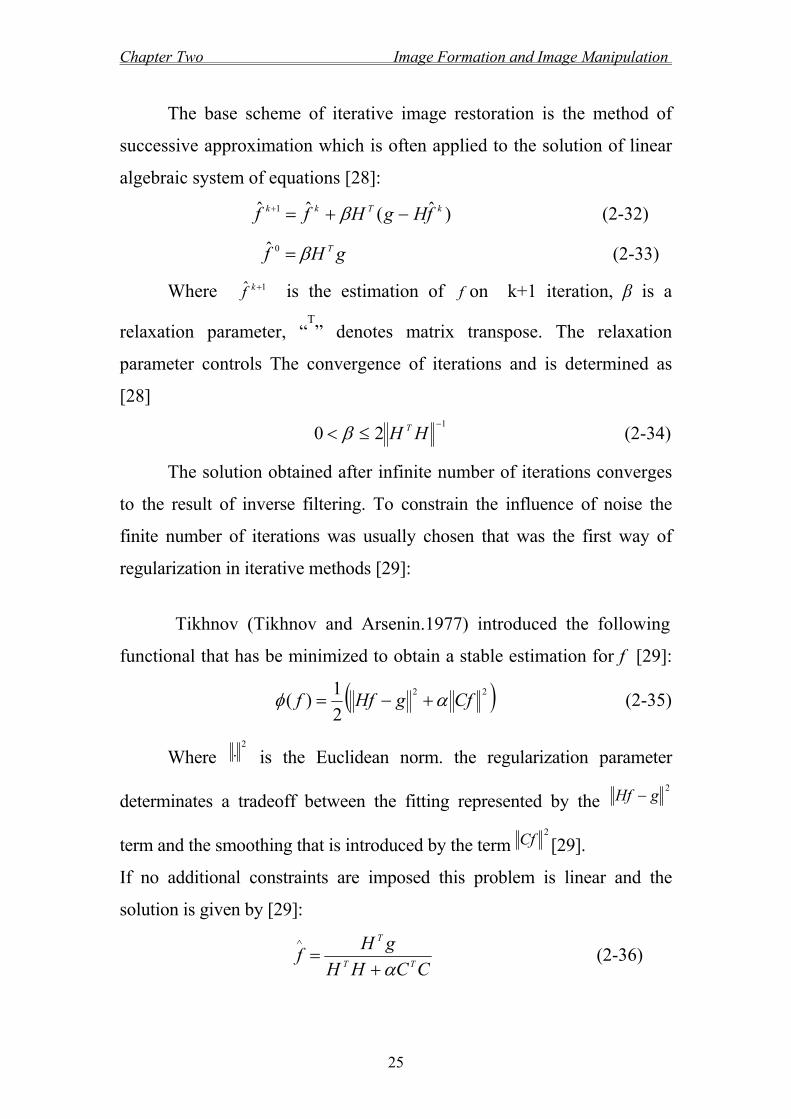
Image Formation and Image Manipulation Chapter Two
25
The base scheme of iterative image restoration is the method of
successive approximation which is often applied to the solution of linear
algebraic system of equations [28]:
)ˆ(ˆˆ 1 kTkk fHgHff (2-32)
gHf T0ˆ (2-33)
Where 1ˆ kf is the estimation of f on k+1 iteration, β is a
relaxation parameter, “T” denotes matrix transpose. The relaxation
parameter controls The convergence of iterations and is determined as
[28]
1
20
HH T (2-34)
The solution obtained after infinite number of iterations converges
to the result of inverse filtering. To constrain the influence of noise the
finite number of iterations was usually chosen that was the first way of
regularization in iterative methods [29]:
Tikhnov (Tikhnov and Arsenin.1977) introduced the following
functional that has be minimized to obtain a stable estimation for f [29]:
(2-35) 22
2
1)( CfgHff
Where 2
. is the Euclidean norm. the regularization parameter
determinates a tradeoff between the fitting represented by the 2
gHf
term and the smoothing that is introduced by the term
2Cf [29].
If no additional constraints are imposed this problem is linear and the
solution is given by [29]:
CCHH
gHf
TT
T
(2-36)

Image Formation and Image Manipulation Chapter Two
26
The introduction of the general regularization theory into iterative
process allowed to essentially increase the algorithm noise immunity. The
generalized scheme of iterative method with Tikhonov regularization could
be written as [28]:
)ˆ(ˆ)(ˆ 1 kTkTk fHgHfCCIf (2-37)
HgHfCCHHI TkTT ˆ))((
Where α is a regularization parameter, C represents high-pass filter
obtained from Tikhonov stabilization functional, I is unit matrix [28].
The regularization parameter controls the tradeoff between fidelity
to the data and smoothness of the solution, and therefore its determination
is very important issue [30].
The operator C was chosen as the Laplasian operator given as the
mask [28 ]:
010
141
010
(2-38)
The regularized solution after k iterations is given in terms of the
eigenvalues and eigenvectors of the blurring[28].
The corresponded condition for relaxation parameter β is given by
[28]:
1
20
CCHH TT (2-39)
Katsaggelos et al. recognize that the term ( I − αβ CTC) behaves
like a low – pass filter, suppressing the noise amplification in the iterates.
As the characteristics of this stabilizing term are obviously related to the
properties of the original image, they proposed to compress this term into
one single low pass operator Cs, which would reflect spectral knowledge
about the original image[28].

Image Formation and Image Manipulation Chapter Two
27
where CS = I − αβ CTC. It was proposed to change it on Wiener
filter for optimal filtering[28].
)ˆ(ˆˆ 1 kTkS
k fHgHfCf (2-40)
HgHfHHC TkT
S ˆ)(
The propose to consider the regularization as a generalized
smoothing of the image that could be accomplished by any known
method of noise removal.
One choice for CS is the noise smoothing wiener filter, which assume
the form[28]:
1)( mnffffS SSSC (2-41)
where S ff and Snn are covariance matrices(autocorrelation
matrices)[27], of the initial image and noise, which supposed to be known
apriori. If these matrices were known a priori, it would be possible to use
this information not only for image smoothing, but also for phase retrieval
that could lead to better results [27].
The advantage of eq. (2-40) over eq. (2-37) is that the interpretation
of (2-40) is more clear. In practice construction of a suitable filter, CS is
sometimes earlier than the selection of regularizing operator C [27].
Another methods for incorporating deterministic constrains into the
restoration process is to extend the basic iterations which is given [27]:
)]ˆ(ˆ)[(ˆ 1 kTkTk fHgHfCCIPf
Where P is again a projection onto a convex set C.
The equation ( 42-2 ) is usually small, the number of constraints
,and the convergence speed[27].
(2-42)

Image Formation and Image Manipulation Chapter Two
28
3.5 Image Quality
In image processing systems, certain amount of errors in the
restored image is tolerated. In this case fidelity criterion can be used as a
measure of system quality. Objective measures or quantitative tests of
image quality can be classified into two classes; these are uni-variant and
bi-variant measures .The uni-variant measure is a numerical rating
assigned to a single image, while the bi-variant measure is a numerical
comparison between pair of images. Since in our research, the problem is
to measure the fidelity of a restoration method where a pair of images
can, always, be provided (i.e. original and restored images), thus we shall
turn our concern to describe some of the bi-variant measures [8].
The quality required naturally depends on the purpose for which
an image is used [ 3].
Methods for assessing image quality can be divided into two
categories [ 3 ]:
1- Objective
2- Subjective
The objective fidelity criteria are borrowed from digital signal
processing and information theory and provide us with equations that
can be used to measure the amount of error in the reconstructed image.
Commonly used objective measures are Root Mean Squares Error
"MSE" signal-to-noise ratio , and the peak signal-to-noise ratio
(SNRpeak) [6].
If we assume that f(x, y) =the original image
),(ˆ yxf =the reconstructed image.
RMSSNR

Image Formation and Image Manipulation Chapter Two
29
The error between an input image f(x,y) and corresponding
restored image ),(ˆ yxf ) is given by[8]:
(2-43) ),(),(),( yxfyxfyxe
The squared error averaged over the image array is then
(2-44)
1
0
1
0
2 ),(1 N
x
M
y
yxeMN
MSE
21
0
1
0
),(),(1
N
x
M
y
yxfyxfMN
MSE (2-45)
21
0
1
02
),(),(ˆ1
N
y
N
x
yxfyxfN
RMSE (2-46)
The smaller the value of the error metrics, the better the
reconstructed image represents the original image.
Alternately, with the signal to noise value, a large number imply a
better image. The (SNR) value consider the reconstructed image ),( vuf
To be the "signal" and error to be the "noise" .We can define the
mean –square signal to noise ratio as[3]:
1
0
1
0
2
1
0
1
0
2
),(),(ˆ
),(ˆ
N
x
N
y
N
x
N
y
RMS
yxfyxf
yxfSNR (2-47)
The root-mean-square error is found by taking the square root of
the error squared divided by the total number of pixels in the image [5]:

Image Formation and Image Manipulation Chapter Two
30
Another related value, the peak signal-to noise ratio, is define as:
1
0
1
0
2
2
2
10
),(),(ˆ1)1(
log10N
x
N
y
peak
yxfyxfN
LSNR (2-48)
Where L the number of grey levels
(e.g. for 8 bits L=256).
It is important to define the ratio of signal to noise in a way which is
consistent with the nature of optical images. The signal to noise ratio "SNR"
can be defined as the ratio of signal variance ( ) to that of the
noise variance ( ) [ 3]:
(2-49)2
2
n
fSNR
where
22 fff
22 nnn
is the mean.
f = the original signal
n = the noise signal.
Since 0n , therefore 22 nn
Subjective fidelity criteria require the definition of a qualitative scale
to assess image criteria. The results are then analyzed statistically,
typically using the averages and standard deviations as metrics. Subjective
fidelity measures can be classified into three categories:
1- They are referred to as impairment tests, where the test subjects in
terms of how bad they are.
2f
2n

Image Formation and Image Manipulation Chapter Two
31
2- The quality tests, where the test subjects rate the images in terms of
how good they are.
3- The comparison tests, where the image are evaluated on a side-by-side
basis.
The subjective measure are better method for comparison of
reconstructed algorithms, if the goal is to achieve high quality images as
defined by our visual perception [6].
For this reason, normalize Cross Correlation Coefficient "CCC" is
given by [ 3 ] :
2
122
),(ˆ),(),(),(
),(ˆ),(),(ˆ),(
yxfyxfyxfyxf
yxfyxfyxfyxfCCC
(2-51)2/1
1
CCC
CCCSNR
where f(x,y) = is the standard or ideal image .
),( yxf is an approximation of the standard field.
The range of CCC is between (-1 to 1). If CCC =1, the imply perfect
correlation (i.e. ),(ˆ yxf = f(x,y)) , (1-c) is measure of the error. The SNR in terms
of C is imply given by [3]:
(2-50)

Results and Discussions Chapter Three
31
CHAPTER THREE

Results and Discussions Chapter Three
32
3.1 Introduction
There are many sources of blur. The focusing atmospheric turbulence blur
which arises, e.g., in remote sensing and astronomical imaging due to short and
long-term exposures through the atmosphere. The turbulence in the atmosphere
gives rise to random variations in the refractive index. For many practical
purposes, and for long exposure, this blurring can be modeled by a Gaussian point
spread function [31].
The purpose of image restoration is to "compensate for" or "undo" defects
which degrade an image. Degradation comes in many forms such as motions blur
noise. In cases like motion blur, it is possible to come up with a very good estimate
of the actual blurring function and "undo" the blur to restore the original image. In
this research, introduce and implement several of the methods are used in the
image processing world to restore images.
Linear methods of image restoration are usually capable of being
computed in a straight forward and economical [32].
Nonlinear methods of image restoration are usually requiring much more
elaborate and closely computational procedures [32].
The Matlab language has been used to restoration image for satellite image
with image size 256 x 256 pixels. The different types of restoration filters are
adapted, these are, Inverse filter, Least-Squares Filter (Wiener filter), Constrained
Least-Squares Filter (Regular Filter), and Iterative restoration (Tikhonov filter).

Results and Discussions Chapter Three
33
3.2 Practical Part
In this chapter, the different types of restoration filters can be adopted, these are:
1. Inverse filter
2. Least-Squares Filter (Wiener filter)
3. Constrained Least-Squares Filter (Regular Filter)
4. Iterative restoration(Tikhonov filter)
Also, Gaussian PSF were adopted with different standards deviation values " σ ",
σ = 0.5, 1, and 2.
Also, have been used two different type of noise these are:
1. Gaussian noise, with different noise level i.e. different SNR, SNR=5, 10,
and 20, with zero mean.
2. Salt and pepper noise, with different noise density "d", d =0.05, and 0.1.
Moreover, we have been used different regularization parameter "α" α =
0, and 0.5.
All restoration techniques are used with image size 256 × 256 pixels.
Image Restoration Algorithm
1- Read color image of size 256 × 256 type RGB.
2- Simulate degraded image (blurred and noisy) with different standards deviation
"σ ", and with different noise level.
3- RGB degraded image has been separated to their component, i.e. Red, Green,
and Blue components.
4- Restoration filters are applied to each component of image, (using inverse
filter, Least-Squares Filter (Wiener filter), constrained Least-Squares Filter
(Regular Filter), and iterative restoration (Tikhonov filter) then returned to RGB
image format.
5- Calculate the mean square error (MSE) for each component of restored RGB
image.
Figure (3-1): shows flowchart of the program

Results and Discussions Chapter Three
34
Start
Simulation of Color noisy image
Separate color Image into (R, G, B)
Components
Restored image And
Calculate MSE for R, G, B components
RGB image
restore
Calculate MSE For (RGB) color
image
End
Figure (3-1) Flowchart of Image Restoration Algorithm
Read Color image

Results and Discussions Chapter Three
35
3.3 Results
A color Jpeg image of 256 256 pixels size , "satellite image", as shown in
Figure(3-2),was used to check the quality of the restoration techniques.
Figure(3-2 ) Original satellite image [33].
The degraded (blurred and noisy) images are simulated as follows:
1. The blurred images were simulated by convolving the original image with
Gaussian function of different standard deviation " σ ", σ =0.5, 1, and 2.
2. Random noise of Gaussian distribution with zero means was added to the
blurred image. Different SNR = 5, 10, and 20,Also, noise of salt and
pepper distribution with noise density "d", d = 0.05, and 0.1) was added to
the blurred image.

Results and Discussions Chapter Three
36
Figure (3-3) shows the degraded image with Gaussian blur and Gaussian noise
with different parameter of degradation , where
a : represent degraded image with σ = 0.5, and SNR =5, b : represent degraded
image with σ = 0.5, and SNR =10, and c : represent degraded image with σ = 0.5,
and SNR =20. The figure shows, also, the Mean Square Error (MSE) of the
degraded image with respect to the original image.
(a) (b)
(c)
Figure(3-3) degraded image with σ = 0.5, and SNR =5,10,20 respectively
MSE = 10.4162
MSE = 14.5667
MSE = 8.2159

Results and Discussions Chapter Three
37
Figure (3-4) shows the degraded image with Gaussian blur and Gaussian noise
with different parameter of degradation, where
a : represent degraded image with σ = 1, and SNR =5, b : represent degraded
image with σ = 1, and SNR =10, and c : represent degraded image with σ = 1,
and SNR =20. The figure shows, also, the Mean Square Error (MSE) of the
degraded image with respect to the original image.
(a) (b)
(c)
Figure(3-4) degraded image with σ = 1, and SNR =5,10,20 respectively
MSE = 11.059
MSE = 15.0624
MSE = 8.9195

Results and Discussions Chapter Three
38
Figure (3-5) shows the degraded image with Gaussian blur and Gaussian noise
with different parameter of degradation, where
a : represent degraded image with σ = 2, and SNR =5, b : represent degraded
image with σ = 2, and SNR =10, and c : represent degraded image with σ = 2,
and SNR =20. The figure shows, also, the Mean Square Error (MSE) of the
degraded image with respect to the original image.
(a) (b)
( c )
Figure(3-5) degraded image with σ =1, and SNR =5,10,20 respectively
MSE = 11.8203
MSE = 17.4375
MSE = 13.6742

Results and Discussions Chapter Three
39
Figure (3-6) shows the degraded image with Gaussian blur and with Salt and
Pepper noise with different parameter , where
a : represent degraded image with σ = 0.5, and d =0.05, b : represent degraded
image with σ = 0.5, and d =0.1. The figure shows, also, the Mean Square Error
(MSE) of the degraded image with respect to the original image.
(b) (a)
Figure(3-6) degraded image with σ = 0.5, and Noise density =0.05,0.1 respectively
Figure (3-7) shows the degraded image Gaussian blur ,and with Salt and Pepper
noise with different parameter of degradation , where
a : represent degraded image with σ = 1, and d =0.05, b : represent degraded
image with σ = 1, and d =0.1. The figure shows, also, the Mean Square Error
(MSE) of the degraded image with respect to the original image.
MSE = 18.74
MSE = 31.19

Results and Discussions Chapter Three
40
( c ) (d)
Figure(3-7) degraded image with σ = 1, and Noise density =0.05,0.1 respectively
Figure (3-8) shows the degraded image Gaussian blur and with Salt and Pepper
noise with different parameter of degradation , where
a : represent degraded image with σ = 2, and d =0.05, b : represent degraded
image with σ = 2, and d =0.1. The figure shows, also, the Mean Square Error
(MSE) of the degraded image with respect to the original image.
(a) (b)
Figure(3-8) degraded image
with σ = 2, and Noise density =0.05,0.1 respectively
MSE = 32.26
MSE = 19.44
MSE = 34.97
MSE = 22.394

Results and Discussions Chapter Three
41
Figure (3-9) represent Mean Square Error (MSE) Versus Signal to Noise
Ratio "SNR" , using Gaussian noise for different with SNR= 5,10, and 20 , and
using different sigma "σ", σ = 0.5, 1, and 2 for Gaussian blur.
7
9
11
13
15
17
19
0 5 10 15 20
Mean Sq
uare Error (M
SE)
Signal ‐ to ‐ noise ratio (SNR)
sigma=0.5
sigma=1
sigma=2
Figure(3-9)
Mean Square Error (MSE) Versus Signal to Noise Ratio "SNR".
Figure (3-10) represent Mean Square Error (MSE) Versus Noise Density (d),
using Salt and Pepper noise for different noise density "d", d=0.05, and 0.1 and
using different with of standard deviation "σ", σ =0.5,1, and 2 for Gaussian blur.
15
17
19
21
23
25
27
29
31
33
35
0.04 0.05 0.06 0.07 0.08 0.09 0.1
Mean Square Error (M
SE)
noise density (d)
sigma=0.5
sigma= 1
sigma= 2
Figure(3-10)
Mean Square Error (MSE) Versus Noise Density (d).

Results and Discussions Chapter Three
42
1. Inverse Filter Figure (3-11) represent the restored image of the degraded image with
Gaussian Point Speared Function and Gaussian noise, with σ = 0.5 ,and SNR=5.
a : represent the restored image for red component, b: represent the restored
image for green component, c: represent the restored image for blue component,
and d: represent the restored image for RGB image , using inverse filter. The figure
shows, also, the (MSE) of the degraded image with respect to the original image.
(a) (b)
(c) (d)
Figure(3-11) Restored Image for red, green , blue components of image and RGB image respectively .
MSE = 0.6141
MSE = 0.6154
MSE = 1.8335
MSE = 0.6040

Results and Discussions Chapter Three
43
Figure (3-12) represent the restored image of the degraded image with
Gaussian Point Speared Function and Gaussian noise, with σ = 0.5 ,and SNR=20.
a : represent the restored image for red component, b: represent the restored image
for green component, c: represent the restore image for blue component, and
d: represent the restored image for RGB image , using inverse filter. The figure
shows, also, the (MSE) of the degraded image with respect to the original image.
(a) (b)
(c) (d)
Figure(3-12) Restored Image for red, green , blue components of image and RGB image respectively.
MSE = 0.6141 MSE = 0.6154
MSE = 0.6040 MSE = 1.8335

Results and Discussions Chapter Three
44
Figure (3-13) represent the restored image of the degraded image with
Gaussian Point Speared Function and Gaussian noise, with σ = 1 ,and SNR=5.
a : represent the restored image for red component, b: represent the restored image
for green component, c: represent the restored image for blue component, and
d: represent the restored image for RGB image , using inverse filter. The figure
shows, also, the (MSE) of the degraded image with respect to the original image.
(a) (b)
(c) (d)
Figure(3-13) Restored Image for red, green ,blue components of image and RGB image respectively .
MSE =1.6031 MSE = 1.6103
MSE = 4.7918 MSE = 1.5783

Results and Discussions Chapter Three
45
Figure (3-14) represent the restored image of the degraded image with
Gaussian Point Speared Function and Gaussian noise, with σ = 1 ,and SNR=20.
a : represent the restored image for red component, b: represent the restored image
for green component, c: represent the restored image for blue component, and
d: represent the restored image for RGB image , using inverse filter. The figure
shows, also, the (MSE) of the degraded image with respect to the original image.
(a) (b)
(c) (d)
Figure(3-14) Restored Image for red, green , blue components of image and RGB image respectively.
MSE =1.6031 MSE = 1.6103
MSE =4.7918 MSE =1.5783

Results and Discussions Chapter Three
46
Figure (3-15) represent the restored image of the degraded image with
Gaussian Point Speared Function and Salt and Pepper noise, with σ = 0.5 ,and
d=0.05.
a : represent the restored image for red component, b: represent the restored image
for green component, c: represent the restored image for blue component, and
d: represent the restored image for RGB image , using inverse filter. The figure
shows, also, the (MSE) of the degraded image with respect to the original image.
(a) (b)
(c) (d)
Figure(3-15) Restored Image for red, green , blue components of image and RGB image respectively.
MSE = 1.8335 MSE = 0.6040
MSE = 0.6141 MSE = 0.6154

Results and Discussions Chapter Three
47
Figure (3-16) represent the restored image of the degraded image with
Gaussian Point Speared Function and Salt and Pepper noise, with σ = 0.5 ,and
d=0.1 .
a : represent the restored image for red component, b: represent the restored image
for green component, c: represent the restored image for blue component, and
d: represent the restored image for RGB image , using inverse filter. The figure
shows, also, the (MSE) of the degraded image with respect to the original image.
(a) (b)
(c) (d)
Figure(3-16) Restored Image for red, green , blue components of image and RGB image respectively.
MSE = 1.8335 MSE =0.6040
MSE =0.6154 MSE = 0.6141

Results and Discussions Chapter Three
48
Figure (3-17) represent the restored image of the degraded image with
Gaussian Point Speared Function and Salt and Pepper noise, with σ = 1 ,and
d=0.05.
a : represent the restored image for red component, b: represent the restored image
for green component, c: represent the restored image for blue component, and
d: represent the restored image for RGB image , using inverse filter. The figure
shows, also, the (MSE) of the degraded image with respect to the original image.
(a) (b)
(c) (d)
Figure(3-17) Restored Image
for red, green , blue components of image and RGB image respectively.
MSE =4.7918 MSE =1.5783
MSE =1.6103 MSE =1.6031

Results and Discussions Chapter Three
49
Figure (3-18) represent the restored image of the degraded image with
Gaussian Point Speared Function and Salt and Pepper noise, with σ = 1 ,and d=0.1.
a : represent the restored image for red component, b: represent the restored image
for green component, c: represent the restored image for blue component, and
d: represent the restored image for RGB image , using inverse filter. The figure
shows, also, the (MSE) of the degraded image with respect to the original image.
(a) (b)
(c) (d)
Figure(3-18) Restored Image for red, green , blue components of image and RGB image respectively.
MSE =4.7918 MSE =1.5783
MSE =1.6103 MSE =1.6031

Results and Discussions Chapter Three
50
2. Wiener Filter
Figure (3-19) represent the restored image of the degraded image with
Gaussian Point Speared Function and Gaussian noise, with σ = 0.5 ,and SNR=5.
a : represent the restored image for red component, b: represent the restored image
for green component, c: represent the restored image for blue component, and
d: represent the restored image for RGB image ,using Wiener filter. The figure
shows, also, the (MSE) of the degraded image with respect to the original image.
(a) (b)
(c) (d)
Figure(3-19) Restored Image for red, green , blue components of image and RGB image respectively.
MSE =13.7751 MSE = 4.5906
MSE = 4.4473 MSE = 4.7372

Results and Discussions Chapter Three
51
Figure (3-20) represent the restored image of the degraded image with
Gaussian Point Speared Function and Gaussian noise, with σ = 0.5 ,and SNR=20.
a : represent the restored image for red component, b: represent the restored image
for green component, c: represent the restored image for blue component, and
d: represent the restored image for RGB image , using Wiener filter. The figure
shows, also, the (MSE) of the degraded image with respect to the original image.
(a) (b)
(c) (d)
Figure (3-20) Restored Image for red, green , blue components of image and RGB image respectively.
MSE =8.2922 MSE =2.7294
MSE =2.7903 MSE =2.7724

Results and Discussions Chapter Three
52
Figure (3-21) represent the restored image of the degraded image with
Gaussian Point Speared Function and Gaussian noise, with σ = 1 ,and SNR=5.
a : represent the restored image for red component, b: represent the restored image
for green component, c: represent the restored image for blue component, and
d: represent the restored image for RGB image ,using Wiener filter. The figure
shows, also, the (MSE) of the degraded image with respect to the original image.
(a) (b)
(c) (d)
Figure(3-21) Restored Image for red, green , blue components of image and RGB image respectively.
MSE =12.6890 MSE =4.1962
MSE =4.1306 MSE =4.3622

Results and Discussions Chapter Three
53
Figure (3-22) represent the restored image of the degraded image with
Gaussian Point Speared Function and Gaussian noise, with σ = 1 ,and SNR=20.
a : represent the restored image for red component, b: represent the restored image
for green component, c: represent the restored image for blue component, and
d: represent the restored image for RGB image , using Wiener filter. The figure
shows, also, the (MSE) of the degraded image with respect to the original image.
(a) (b)
(c) (d)
Figure(3-22) Restored Image
for red, green , blue components of image and RGB image respectively.
MSE =7.9443 MSE =2.6394
MSE =2.6435 MSE = 2.6613

Results and Discussions Chapter Three
54
Figure (3-23) represent the restored image of the degraded image with
Gaussian Point Speared Function and Salt and Pepper noise, with different
parameter , where
a : represent the restored image of the degraded image with σ = 0. 5 and d=0.05,
b: represent the restored image of the degraded image with σ = 0. 5 ,and d=0.1,
c: represent the restored image of the degraded image with σ = 1 ,and d=0.05,
d: represent the restored image of the degraded image with σ = 1 ,and d=0.1 ,
using Wiener filter. The figure shows, also, the (MSE) of the degraded image with
respect to the original image.
(a) (b)
(c) (d)
Figure(3-23) Restored Image
MSE =18.7674 MSE =14.3029
MSE =16.8919 MSE =26.7891

Results and Discussions Chapter Three
55
3. Constrained Least-Squares Filter (Regular Filter) Figure (3-24) represent the restored image of the degraded image with
Gaussian Point Speared Function and Gaussian noise, with different parameter ,
where
a : represent the restored image of the degraded image with σ = 0. 5 and SNR =5,
b: represent the restored image of the degraded image with σ = 0. 5 and SNR =20,
c : represent the restored image of the degraded image with σ = 1 and SNR =5,
d: represent the restored image of the degraded image with σ = 1 and SNR =20,
using Constrained Least-Squares Filter. The figure shows, also, the (MSE) of the
degraded image with respect to the original image.
(a) (b)
(c) (d)
Figure(3-24) Restored Image
MSE =9.1764 MSE =6.5621
MSE = 6.543 MSE = 4.8399

Results and Discussions Chapter Three
56
Figure (3-25) represent the restored image of the degraded image with
Gaussian Point Speared Function and Salt and Pepper noise, with different
parameter , where
a : represent the restored image of the degraded image with σ = 0. 5 and d=0.05,
b: represent the restored image of the degraded image with σ = 0. 5 ,and d=0.1,
c: represent the restored image of the degraded image with σ = 1 ,and d=0.05,
d: represent the restored image of the degraded image with σ = 1 ,and d=0.1 ,
using Constrained Least-Squares Filter.
The figure shows, also, the (MSE) of the degraded image with respect to the
original image.
(a) (b)
(c) (d)
MSE =10.1128 MSE =12.1251
MSE = 7.2833 MSE =12.6894
Figure(3-25) Restored Image

Results and Discussions Chapter Three
57
4. Iterative Restoration(Tikhonov method )
Figure (3-26a) represent the restored image of the degraded image with
Gaussian Point Speared Function and Gaussian noise, with σ = 0.5 ,and SNR=5.
This figure represent the restored image for RGB image after 6 iterations,
using Tikhonov method. when α = 0.
Figure(3-26a ) Restored image for RGB image after 6 iterations
Figure (3-26b) represent MSE Versus no. of iterations for the restored
image of the degraded image with Gaussian Point Speared Function and Gaussian
noise, with σ = 0.5 ,and SNR=5. For red, green, blue components, and RGB image
, using Iterative Restoration When α =0.
3
5
7
9
11
13
15
0 2 4 6 8
Mean
Square Error (M
SE)
no. of iterations
Red Component
Green Component
Blue Component
RGB
MSE =9.6277
Figure (3-26b) MSE Versus. no. of iterations

Results and Discussions Chapter Three
58
Figure (3-27a) represent the restored image of the degraded image with
Gaussian blur and Gaussian noise, with σ = 0.5 ,and SNR=20 for RGB image ,
using Tikhonov method after 7 iterations. when α = 0 (α: regularization parameter).
Figure (3-27b) represent MSE Versus no. of iterations .
7
7.5
8
8.5
9
9.5
10
0 1 2 3 4 5 6 7
Mean Square Error (M
SE)
no. of iteration
Figure (3-28a) represent the restored image of the degraded image with
Gaussian blur and Gaussian noise, with σ = 1 ,and SNR=5 for RGB image , using
Tikhonov method after 10 iterations. when α = 0 (α: regularization parameter ).
Figure (3-28b) represent MSE Versus no. of iterations .
9.6
9.8
10
10.2
10.4
10.6
10.8
11
11.2
11.4
11.6
0 2 4 6 8 10
Mean Square Error (M
SE)
no. of iteration
Figure (3-28b) MSE VS. no. of iterations when degraded
image with σ =1 , and SNR=5
Figure (3-27b) MSE Versus no. of iterations when degraded
image with σ =0.5 , and SNR=20
Figure (3-27a) MSE = 7.07
Restored image for RGB image after 7 iterations
Figure (3-28a) MSE = 9.86
Restored image for RGB image after 10 iterations

Results and Discussions Chapter Three
59
Figure (3-29a) represent the restored image of the degraded image with
Gaussian blur and Gaussian noise, with σ = 1 ,and SNR=20 for RGB image , using
Tikhonov method after 30 iterations. when α = 0 (α: regularization parameter ).
Figure (3-29b) represent MSE Versus no. of iterations .
8
8.2
8.4
8.6
8.8
9
9.2
9.4
9.6
9.8
10
0 5 10 15 20 25 30
Mean Square Error (M
SE)
no. of iteration
Figure (3-30a) represent the restored image of the degraded image with
Gaussian blur and Salt and pepper noise, with σ = 0.5 ,and d=0.05 for RGB image
,using Tikhonov method after 4 iterations. when α = 0 (α: regularization
parameter).
Figure (3-30b) represent Mean Square Error (MSE) Versus no. of iterations .
11
11.2
11.4
11.6
11.8
12
12.2
12.4
12.6
12.8
13
0 1 2 3 4
Mean Square Error (M
SE)
no. of iteration
Figure (3-29b) MSE VS. no. of iterations when degraded
image with σ =1 ,and SNR=20
Figure (3-30b) MSE VS. no. of iterations when degraded
image with σ =0.5, and d=0.05
Figure (3-29a) MSE = 8.11
Restored image for RGB image after 30 iterations
Figure (3-30a) MSE = 11.209
Restored image for RGB image after 4 iterations

Results and Discussions Chapter Three
60
Figure (3-31a) represent the restored image of the degraded image with
Gaussian blur and Salt and pepper noise, with σ = 0.5 ,and d=0.1 for RGB image ,
using Tikhonov method after 4 iterations. when α = 0 (α: regularization
parameter).
Figure (3-31b) represent MSE Versus no. of iterations .
15
16
17
18
19
20
21
22
23
24
25
0 1 2 3 4
Mean Square Error (M
SE)
no. of iteration
Figure (3-32a) represent the restored image of the degraded image with
Gaussian blur and Salt and pepper noise, with σ = 1 ,and d=0.05 for RGB image ,
using Tikhonov method after 5 iterations. when α = 0 (α: regularization
parameter). Figure (3-32b) represent MSE Versus no. of iterations .
10
11
12
13
14
15
16
17
0 1 2 3 4 5
Mean Square Error (M
SE)
no. of iteration
Figure (3-31b) MSE VS. no. of iterations when degraded
image with σ =0.5, and d=0.1
Figure (3-32b) MSE VS. no. of iterations when degraded image
with σ =1, and d=0.05
Figure (3-31a) MSE = 15.921
Restored image for RGB image after 4 iterations
Figure (3-32a) MSE = 11.071
Restored image for RGB image after 5 iterations

Results and Discussions Chapter Three
61
Figure (3-33a) represent the restored image of the degraded image with
Gaussian blur and Salt and pepper noise, with σ = 1 ,and d=0.1 for RGB image ,
using Tikhonov method after 3 iterations. when α = 0 (α: regularization parameter)
Figure (3-33b) represent MSE Versus no. of iterations .
13
14
15
16
17
18
19
0 1 2 3
Mean Square Error (M
SE)
no. of iteration
Figure (3-34a) represent the restored image of the degraded image with
Gaussian blur and Salt and pepper noise, with σ = 2 ,and d=0.05 for RGB image ,
using Tikhonov method after 17 iterations. When α = 0 (α: regularization
parameter )
Figure (3-34b) represent MSE Versus no. of iterations .
13.2
13.3
13.4
13.5
13.6
13.7
13.8
13.9
14
0 1 2 3 4 5 6 7 8 9 10 11 12 13 14 15 16 17
Mean Square Error (M
SE)
no. of iteration
Figure (3-33b) MSE VS. no. of iterations when degraded
image with σ =1, and d=0.1
Figure (3-34b) MSE VS. no. of iterations when degraded
image with σ =2, and d=0.05
Figure (3-33a) MSE = 14.21
Restored image for RGB image after 3 iterations
Figure (3-34a) MSE =13.294
Restored image for RGB image after 17 iterations

Results and Discussions Chapter Three
62
Figure (3-35a) represent the restored image of the degraded image with
Gaussian blur and Gaussian noise, with σ = 0.5 ,and SNR=5 for RGB image , using
Tikhonov method after 7 iterations. when α = 0.5 (α: regularization parameter ).
Figure (3-35b) represent MSE Versus no. of iterations .
9
9.5
10
10.5
11
11.5
12
12.5
13
13.5
0 1 2 3 4 5 6 7
Mean Square Error (MSE)
no. of iteration
Figure (3-36a) represent the restored image of the degraded image with
Gaussian blur and Gaussian noise, with σ = 0.5 ,and SNR=20 for RGB image ,
using Tikhonov method after 8 iterations. when α = 0.5 (α: regularization
parameter ).
Figure (3-36b) represent MSE Versus no. of iterations .
7
7.5
8
8.5
9
9.5
10
0 1 2 3 4 5 6 7 8
Mean Square Error (M
SE)
no. of iteration
Figure (3-35b) MSE VS. no. of iterations when degraded
image with σ =0.5 ,and SNR=5
Figure (3-36b) MSE VS. no. of iteration s when degraded image
with σ =0.5 , and SNR=20
Figure (3-35a) MSE = 9.7
Restored image for RGB image after 7 iterations
Figure (3-36a) MSE = 7.1264
Restored image for RGB image after 8 iterations

Results and Discussions Chapter Three
63
Figure (3-37a) represent the restored image of the degraded image with
Gaussian blur and Gaussian noise, with σ = 1 ,and SNR=5 for RGB image , using
Tikhonov method after 9 iterations. when α = 0.5 (α: regularization parameter ).
Figure (3-37b) represent MSE Versus no. of iterations .
9
10
11
12
13
14
15
16
17
0 1 2 3 4 5 6 7 8 9
Mean Square Error (M
SE)
no. of iteration
Figure (3-38a) represent the restored image of the degraded image with
Gaussian blur and Gaussian noise, with σ = 1 ,and SNR=20 for RGB image , using
Tikhonov method after 30 iterations. when α = 0 (α: regularization parameter ).
Figure (3-38b) represent MSE Versus no. of iterations .
8
8.2
8.4
8.6
8.8
9
9.2
9.4
9.6
9.8
10
0 5 10 15 20 25 30
Mean Square Error (M
SE)
no. of iteration
Figure (3-37b) MSE VS. no. of iterations when degraded
image with σ , and SNR=5
Figure (3-38b) MSE VS. no. of iterations when degraded
image with σ =1 , and SNR=20
Figure (3-37a) MSE = 9.8214
Restored image for RGB image after 9 iterations
Figure (3-38a) MSE = 8.155
Restored image for RGB image after 30 iterations

Results and Discussions Chapter Three
64
Figure (3-39a) represent the restored image of the degraded image with
Gaussian blur and Salt and pepper noise, with σ = 0.5 ,and d=0.05 for RGB image
,using Tikhonov method after 4 iterations. when α = 0.5 (α: regularization
parameter ). Figure (3-39b) represent MSE Versus no. of iterations .
10.8
11
11.2
11.4
11.6
11.8
12
12.2
12.4
12.6
0 1 2 3 4
Mean Square Error (MSE)
no. of iteration
Figure (3-40a) represent the restored image of the degraded image with
Gaussian blur and Salt and pepper noise, with σ = 0.5 ,and d=0.1 for RGB image ,
using Tikhonov method after 4 iterations. when α = 0.5 (α: regularization
parameter ). Figure (3-40b) represent MSE Versus no. of iterations .
15
16
17
18
19
20
21
22
23
24
25
0 1 2 3 4
Mean Square Error (M
SE)
no. of iteration
Figure (3-39b) MSE VS. no. of iterations when degraded
image with σ =0.5 , and d=0.05
Figure (3- 40b) MSE VS. no. of iterations when degraded
image with σ =0.5 , and d=0.1
Figure (3- 39a) MSE = 10.9595
Restored image for RGB image after 4 iterations
Figure (3-40a) MSE = 15.32061
Restored image for RGB image after 4 iterations

Results and Discussions Chapter Three
65
Figure (3-41a) represent the restored image of the degraded image with
Gaussian blur and Salt and pepper noise, with σ = 1 ,and d=0.05 for RGB image ,
using Tikhonov method after 5 iterations. when α = 0.5 (α: regularization
parameter ). Figure (3-41b) represent MSE Versus no. of iterations .
10
11
12
13
14
15
16
0 1 2 3 4 5
Mean Square Error (M
SE)
no. of iteration
Figure (3-42a) represent the restored image of the degraded image with
Gaussian blur and Salt and pepper noise, with σ = 1 ,and d=0.1 for RGB image ,
using Tikhonov method after 3 iterations. when α = 0.5 (α: regularization
parameter ). Figure (3-42b) represent MSE Versus no. of iterations .
13
14
15
16
17
18
19
0 1 2 3
Mean Square Error (M
SE)
no. of iteration
Figure (3-41b) MSE VS. no. of iterations when degraded
image with σ =1 , and d=0.05
Figure (3-42b) MSE VS. no. of iterations when degraded
image with σ =1 , and d=0.1
Figure (3-41a) MSE = 10.78
Restored image for RGB image after 5 iterations
Figure (3-42a) MSE = 14.0196
Restored image for RGB image after 3 iterations

Results and Discussions Chapter Three
66
Figure (3-43) represent MSE Versus no. of iterations for restored image of
degraded image with Gaussian Point Speared Function and Gaussian noise, with σ
= 0.5 ,and SNR=5. when α = 0.5, and α = 0.
9
9.5
10
10.5
11
11.5
12
12.5
13
13.5
0 2 4 6 8
Mean Square Error (M
SE)
no. of iteration
α=0.5
α= 0
Figure (3-44) represent MSE Versus no. of iterations for restored image of
degraded image with Gaussian Point Speared Function and Gaussian noise, with σ
= 0.5 ,and SNR=10. when α = 0.5, and α = 0.
7.5
8
8.5
9
9.5
10
10.5
11
11.5
12
0 2 4 6 8
Mean Sq
uare Error (M
SE)
no. of iteration
α= 0.5
α= 0
Figure (3- 43 ) MSE VS. no. of iteration
when degraded image with Gaussian PSF and Gaussian noise with σ =0.5 ,and SNR =5
Figure (3- 44 ) MSE VS. no. of iteration
when degraded image with Gaussian PSF and Gaussian noise with σ =0.5 ,and SNR =10

Results and Discussions Chapter Three
67
Figure (3-45) represent MSE Versus no. of iterations for restored image of
degraded image with Gaussian Point Speared Function and Gaussian noise, with σ
= 0.5 ,and SNR=20. when α = 0.5, and α = 0.
7
7.5
8
8.5
9
9.5
10
10.5
0 2 4 6 8 10
Mean Square Error (M
SE)
no. of iteration
α = 0 .5
α = 0
Figure (3-46) represent MSE Versus no. of iterations for restored image of
degraded image with Gaussian Point Speared Function and Gaussian noise, with σ
= 1 ,and SNR=5. when α = 0.5, and α = 0.
9
10
11
12
13
14
15
16
0 2 4 6 8 10
Mean Square Error (M
SE)
no. of iteration
α = 0.5
α = 0
Figure (3- 45 ) Mean Square Error VS. no. of iteration
when degraded image with Gaussian PSF and Gaussian noise with σ =0.5 ,and SNR =20
Figure (3- 46 ) MSE VS. no. of iteration
when degraded image with Gaussian PSF and Gaussian noise with σ =1 ,and SNR =5

Results and Discussions Chapter Three
68
Figure (3-47) represent MSE Versus no. of iterations for restored image of
degraded image with Gaussian Point Speared Function and Gaussian noise, with σ
= 1 ,and SNR=10. when α = 0.5, and α = 0.
8.6
8.8
9
9.2
9.4
9.6
9.8
10
10.2
10.4
10.6
0 5 10 15 20
Mean Square Error (M
SE)
no. of iteration
α = 0.5
α = 0
Figure (3-48) represent MSE Versus no. of iterations for restored image of
degraded image with Gaussian Point Speared Function and Gaussian noise, with σ
= 1 ,and SNR=20. when regularization parameter " α", α = 0.5, and α = 0.
8
8.2
8.4
8.6
8.8
9
9.2
9.4
9.6
9.8
10
0 5 10 15 20 25 30 35
Mean Sq
uare Error (M
SE)
no. of iteration
α = 0.5
α = 0
Figure (3- 47 ) MSE VS. no. of iteration
when degraded image with Gaussian PSF and Gaussian noise with σ =1,and SNR =10
Figure (3- 48 ) MSE VS. no. of iteration
when degraded image with Gaussian PSF and Gaussian noise with σ =1,and SNR =20

Results and Discussions Chapter Three
69
Figure (3-49) represent MSE Versus no. of iterations for restored image of
degraded image with Gaussian Point Speared Function and Gaussian noise, with σ
= 2 ,and SNR=5. when α = 0.5, and α = 0.
12
12.2
12.4
12.6
12.8
13
13.2
13.4
13.6
13.8
14
0 5 10 15 20 25 30 35
Mean Square Error (M
SE)
no. of iteration
α = 0.5
α = 0
Figure (3-50) represent MSE Versus no. of iterations for restored image of
degraded image with Gaussian Point Speared Function and Gaussian noise, with σ
= 2 ,and SNR=10. α = 0.5, and α = 0.
11.4
11.9
12.4
12.9
13.4
13.9
0 10 20 30 40
Mean Squa
re Error (M
SE)
no. of iteration
α = 0.5
α = 0
Figure (3- 49 ) MSE VS. no. of iteration
when degraded image with Gaussian PSF and Gaussian noise with σ =2,and SNR =5
Figure (3- 50 ) MSE VS. no. of iteration
when degraded image with Gaussian PSF and Gaussian noise with σ =2,and SNR =10

Results and Discussions Chapter Three
70
Figure (3-51) represent MSE Versus no. of iterations for restored image of
degraded image with Gaussian Point Speared Function and Gaussian noise, with σ
= 2 ,and SNR=20. when α = 0.5, and α = 0.
11
11.2
11.4
11.6
11.8
12
12.2
0 5 10 15 20 25 30
Mean Square Error (M
SE)
no. of iteration
α = 0.5
α = 0
Figure (3-52) represent MSE Versus no. of iterations for restored image of
degraded image with Gaussian Point Speared Function and Salt and Pepper noise,
with σ = 0.5 ,and d=0.05. when α = 0.5, and α = 0.
10.5
11
11.5
12
12.5
13
0 1 2 3 4
Mean
Square Error (M
SE)
no. of iteration
α = 0.5
α = 0
Figure (3- 51 ) MSE VS. no. of iterations
when degraded image with Gaussian PSF and Gaussian noise with σ =2,and SNR =20
Figure (3- 52 ) MSE VS. no. of iteration when degraded image with Gaussian
PSF and Salt and pepper noise with σ =0.5 ,and d =0.05

Results and Discussions Chapter Three
71
Figure (3-53) represent MSE Versus no. of iterations for restored image of
degraded image with Gaussian Point Speared Function and Salt and Pepper noise,
with σ = 0.5 ,and d=0.1. when α = 0.5, and α = 0.
15
16
17
18
19
20
21
22
23
24
25
0 1 2 3 4
Mean
Square Error (M
SE)
no. of iteration
α = 0.5
α = 0
Figure (3-54) represent MSE Versus no. of iterations for restored image of
degraded image with Gaussian Point Speared Function and Salt and Pepper noise,
with σ = 1 ,and d=0.05. when α = 0.5, and α = 0.
10.5
11.5
12.5
13.5
14.5
15.5
16.5
17.5
0 1 2 3 4 5
Mean
Square Error (M
SE)
no. of iteration
α = 0.5
α = 0
Figure (3- 53 ) MSE VS. no. of iterations when degraded image with Gaussian
PSF and Salt and pepper noise with σ =0.5 ,and d =0.1
Figure (3-54) MSE VS. no. of iterations when degraded image with Gaussian
PSF and Salt and pepper noise with σ =1 ,and d =0.05

Results and Discussions Chapter Three
72
Figure (3-55) represent MSE Versus no. of iterations for restored image of
degraded image with Gaussian Point Speared Function and Salt and Pepper noise,
with σ = 1 ,and d=0.1. when α = 0.5, and α = 0.
13.6
14.1
14.6
15.1
15.6
16.1
16.6
17.1
17.6
18.1
18.6
0 1 2 3
Mean Sq
uare Error (M
SE)
no. of iteration
α = 0.5
α = 0
Figure (3-56) represent MSE Versus no. of iterations for restored image of
degraded image with Gaussian Point Speared Function and Salt and Pepper noise,
with σ = 2 ,and d=0.05. when α = 0.5, and α = 0.
15.25
15.3
15.35
15.4
15.45
15.5
15.55
15.6
15.65
15.7
15.75
15.8
0 2 4 6 8
Mean Squa
re Error (M
SE)
no. of iteration
α = 0.5
α = 0
Figure (3- 55) MSE VS. no. of iterations when degraded image with Gaussian PSF
and Salt and pepper noise with σ =1 ,and d =0.1
Figure (3- 56) MSE VS. no. of iterations when degraded image with Gaussian
PSF and Salt and pepper noise with σ =2 ,and d =0.05

Results and Discussions Chapter Three
73
Figure (3-57) represent MSE Versus no. of iterations for restored image of
degraded image with Gaussian Point Speared Function and Salt and Pepper noise,
with σ = 2 ,and d=0.1. when α = 0.5, and α = 0.
13.1
13.2
13.3
13.4
13.5
13.6
13.7
13.8
13.9
14
14.1
0 1 2 3 4 5 6 7 8 9 10 11 12 13 14 15 16 17Mean
Square Error (M
SE)
no. of iteration
α = 0.5
α = 0
Figure (3- 57) MSE VS. no. of iterations when degraded image with Gaussian
PSF and Salt and pepper noise with σ =2 ,and d =0.1

Results and Discussions Chapter Three
74
3.4 Results Discussion
Table(3-2) shows the MSE of restored images with different type of filter
σ SNR=5 MSE
SNR=10 MSE
SNR=20 MSE
0.5 14.5667 10.4162 8.2159
Degraded
1 15.0624 11.059 8.9195
image 2 17.4375 13.6742 11.8203
Restored image 0.5 1.8335 1.8335 1.8335
Using 1 4.7918 4.7918 4.7918
Inverse Filter 2 8.6283 8.6283 8.6283
Restored image 0.5 13.7751 10.0890 8.2922
Using 1 12.6890 9.2262 7.9443
Wiener Filter 2 14.6580 10.8900 9.5106
Restored image 0.5 6.543 5.9603 4.8399
Using 1 9.1764 7.5827 6.5621
Regular Filter 2 17.4571 10.0362 9.2042
Restored image 0.5 9.6277 After 6 iterations
7.95 After 6 iterations
7.07 After 7 iterations
Using Tikhonov Filter
1 9.86 After 10 iterations
8.774 After 16 iterations
8.11 After 30 iterations
When α = 0 2 12.08 After 30 iterations
11.42 After 30 iterations
11.14 After 30 iterations
Restored image 0.5 9.7 After 7 iterations
8.009 After 8 iterations
7.1264 After 8 iterations
Using Tikhonov Filter
1 9.8214 After 9 iterations
8.753 After 18 iterations
8.155 After 30 iterations
When α = 0.5 2 12.115 After 6 iterations
11.4309 After 6 iterations
11.246 After 6 iterations

Results and Discussions Chapter Three
75
Table(3-2) shows the MSE of restored images with different type of filter.
From the Tables (3-1),and (3-2) can be discussed:
• The degraded (blurred and noisy) images are simulated as follows:
σ d =0.05 MSE
d =0.1 MSE
0.5 18.74 31.19
Degraded
1 19.44 32.26
image 2 22.394 34.97
Restored image 0.5 1.8335 1.8335
Using 1 4.7918 4.7918
Inverse Filter 2 8.6283 8.6283
Restored image 0.5 16.8919 26.7891
Using 1 14.3029 18.7674
Wiener Filter 2 15.1719 16.6094
Restored image 0.5 7.2833 12.6894
Using 1 12.1251 10.1128
Regular Filter 2 15.8194 13.1138
Restored image 0.5 11.209 After 4 iterations
15.921 After 4 iterations
Using Tikhonov Filter
1 11.071 After 5 iterations
14.21 After 3 iterations
When α = 0 2 13.294 After 17 iterations
15.34 After 6 iterations
Restored image 0.5 10.9595 After 4 iterations
15.32061 After 4 iterations
Using Tikhonov Filter
1 10.78 After 5 iterations
14.0196 After 3 iterations
When α = 0.5 2 13.2124 After 17 iterations
15.3245 After 7 iterations

Results and Discussions Chapter Three
76
1. The blurred images were simulated by convolving the original image
with Gaussian function of different standard deviation (σ =0.5, 1, and
), one values of a =1 has been taken.
2. Random noise of Gaussian distribution with zero means was added to
the blurred image (obtained in step 1). Different SNR = 5 dB, 10 dB,
and 20dB, and noise of salt & pepper distribution with noise density(d
= 0.05, and 0.1) was added to the blurred image (obtained in step 1),
have been taken.
Figures (3-9),and(3-10),were mean square error vs. SNR and noise
density respectively, and show that mean square error its decreased with SNR
and increasing with noise density.
To restore the above simulated degraded images,
• The MSE of restored image by using regular filter it is less than Weiner filter
and Tikhonov filter , when σ =2 and SNR= 5.i.e. when degraded image with
high degraded parameters.
• The MSE of restored image by using Tikhonov filter when σ = 2 and SNR=
Sit is less than other filter except inverse filter.
• The MSE of restored image for corrupted with salt and pepper noise by
using regular filter when σ = 2and d=0.05, it is less than Weiner filter and
Tikhonov filter.
• The MSE of restored image for corrupted with salt and pepper noise by
using regular filter when σ =2 and d=0.1, it is less than Weiner filter and
Tikhonov filter.
• The values of MSE of restored image by using Tikhonov filter it is
different, when σ =0, and a =0.5, with different types of noise.
• The number of iterations increased with increasing the degradation
parameters.
• Iterative algorithms are normally slow to converge, some of its high
computational requirement.

Conclusions and Future Work Chapter Four
76
CHAPTER FOUR

Conclusions and Future Work Chapter Four
77
4.1 Conclusions
From our results of this research, some notes can be conclude:
1. Tikhonov method was used, the MSE of the restored images
decreases with increasing the number of iteration until the result
convergence. Also, the ratio of the MSE of the degraded image to
the MSE of the restored image will increased with increasing SNR,
i.e. this method has better performance for less degradation
parameters, with high SNR.
2. The ratio of the MSE of the degraded image (corrupted with salt
and pepper noise) to the MSE of the restored image will increased
with increasing noise density. This method has better performance
for large degradation parameters with high noise density.
3. The Tikhonov methods, causes edge blurring.
4. The values of the regularization parameter (α) depend on the type
of the noise.
Suggest For Future Work 4.2
From the work of this research, some notes can be suggested as
future work:
1. It is quite interesting for future work, to use a nonlinear technique
of image restoration to restore the real an astronomical data and
compare results to be obtained with simple technique.
2. Using nonlinear iterative restoration and compare the results with
another kind of iterative image restoration. Such as maximum
entropy method, POC methods.
3. Using nonlinear iterative restoration with different the relaxation
parameter.

References
77

References
78
1. J. Teuber , " Digital Image Processing", First ed., Prentice Hall
International(UK)Ltd.(1993).
2. R. Gonzales , and P. Wintz ," Digital Image Processing", Addison-
Wesley publishing, (2000).
3. M. I. Abd - Almajied," Image Restoration of Multispectral Satellite
Images", M.Sc. Thesis, University of Baghdad,(2006).
4. A. Jain ,"Fundamental of Digital Image Processing", Prentice
Hall,(1998).
5. R. Gonzales, and R. Wood ," Digital Image Processing", Fifth ed.,
Pearson Education Asia Pte Ltd,(2000).
6. S. Umbagh ," Computer Vision and Image Processing", Prentice Hall
PTR,(1998).
7. S. A. H. Salih, "Theoretical Limits of the Application of an Image
Restoration Technique in Astronomy" ,M.Sc. Thesis, University of
Wals,(1983).
8. N. M. O. Al- Shareefi, "Restoration of Astronomical Image Using
Adaptive Kalman Filter", M.Sc. thesis, University of Baghdad,(2000).
9. A. Rosenfeld, and A. C. Kak," Digital Picture Processing ", Academic
Press , Inc,(1976).
10. W. K. Pratt ," Digital Image Processing", Jhon Wiley & Sons. Inc.
Canada, (1978).
11. D. Angwin, and H.Kaufman," Adaptive Restoration of Color Image",
Decision and Control ,Vol. 26, Part 1,1987 Page(s):1196 – 1197.
12. G. M. P. van Kempen, and L.J. Van Viliey, "The influence of the
Background Estimation on the Super resolution Properties of Non-
Linear Image Restoration ", Image Acquisition and
Processing,vol.6,pp.179-189,(1999)
13. G. M. P.van Kempen , and L.J. Van Viliey, "The influence of the
Regularization parameter and The First Estimation on the Performance

References
79
of Tikhonov Regularization Non-Linear Image Restoration Algorithms ",
Journal Of Microscopy,,vol.198,pp.63-75,(2000)
14. H. Wu, H. J. Zhang, and Z.Liu, " Fast Image Restoration in Large
Digital Photo", Digital Object Identifier, Vol. 1, 15-18 ,pp.537 - 540 ,
(2003).
15. S. H. Lee, N. I. Cho, and J.II Park ,"Directional Regularization for
Constrained Iterative Image Restoration ", Electronic letters,vol.39 ,
no.23(2003)
16. S. W. Perry, and P. Varjavandi, and L. Guan, " Adaptive Image
Restoration Using a Perception Based Error Measurement",(2004)
www.ewh.ieee.org/reg/7/ccece04/program-weal-vz.pdf.
17. Y. H. Chan, and Y. H. Fung, " A Regularized Constrained Iterative
Restoration Algorithm for Restoring Color Quantized Images", Signal
Processing, vol. 85, pp. 1375- 1387,(2005)
18. Q. S. F. Xue, and W. fan ,"Iterative Image Restoration Using a non –
local Regularization Function and a local Regularization Operator ", 18
th International Conference on Pattern Recognition ,vol.3,pp.766-
769(2006)
19. P. Favati, O. Menchi, G. Lotti., and F.Romani "Iterative Image
Restoration with non negativity Constraints",(2006)
http://dienst.isti.cnr.it/dienst/ui/2.0/describe/ercim.cnr.iit/2006-TR-
010/tiposearch=cnr=&langre
20. A. Alani, " Restoration of Astronomical Image Using an Adaptive
Iterative Wiener Filter", Journal of AL-Nahrain University, College of
Science, (2006).
21. T. F. Chan, K. Chen, and J. L. Carter, " Iterative Methods for
Solving the Dual Formulation Arising From Image Restoration",
Electronic Transaction on Numerical Analysis, vol. 26, pp. 299-
311,(2007).

References
80
22. W. Zhao, A. Pope," Image Restoration Under Signifcant Additive
Noise", IEEE Signal Processing letters, vol. 14, No.6, pp.401- 404,
(2007).
23. R. L. Lagendijk, and J. Biemond, " Basic Methods for Image
Restoration and Indentification", Academic press, (2000).
24. A. Smirnov, and M. Ginzburg," Iterative Image Restoration"
I/DIP/VisionClasses/done_Projects/Project/Isl/Labs/il.ac.technion.cs.www://http/Restoration_terative
25. R. Gonzales, R. E.Wood , and S. L. Edding ," Digital Image
Processing Using Matlab ", Prentice Hall,(2004).
26. A. K. Kustsggelos, and M.G. Kang," Iterative Evaluation of the
Regularization Parameter in Regularized Image Restoration", Journal of
Visual Communication and Image Representation, vol.3 , No.4, pp. 446-
459,(1995).
27. J. Biemond, R. L. Lagendijk, and R. M. Mersereau," Iterative
Methods for Deblurring", Processdings of the IEEE, vol. 78, No.5,
pp.856-883, (1990).
28. S. Voloshynovskiy, " Iterative Image Restoration With Adaptive
Regularization and Parametric Constraints", Journal of Image
Processing and Communication, vol. 3, 3-4, pp. 73-88, (1997).
29. P. J. Verveer, and T. M. Jovin," Accelaration of ICTM Image
Restoration Algorithm", Journal of Microscopy, vol. 188, pt3, pp. 191-
195,(1997).
30. K. G. Kang, and A. K. Kustsggelos," Simultaneous Iterative Image
Restoration and Evaluation of Regularization Parameter", IEE
Transaction on signal processing, vol. 40, No. 4, pp. 2329-2334, (1992).
31. P. C. Hansen," Digital Image Restoration",
html.pptsvd/PPTSVD/pch~/dk.dtu.imm.2www://http 32. H. C. Andrews and B. R. Hunt, " Digital Image Restoration", Prentice
Hall, Englewood Cliffs, N. J., (1977).
33. http://www.lakii.com/vb/showthread.php?t=240961

الخلاصة لعمليات التد�ي وهي عملية معاكسة لعمليـات التـد�ي تقريبـا ةترميم الصور هي عملية �تيجة تقريبي
.لتقدير الصورة الأصلية وهي عمليات معاكسة لعمليات التد�ي تقريبا لتقدير الصورة الأصليةورة فضائية ملو�ة صمم لترميم ص) Tikhonovطريقة (المرشح المتبنيتقنية الترميم التكرارية ،
& Salt ومـشوشة بـضجيج كـاوس و ) دالة كـاوس (مغوشة بضوضاء ثابت الفضائي دالة النشر النقطية
Pepper بأختلاف معاملات التـد�ي ، بعبـارة أخـرى بـأختلاف �ـسبة الأشـارة الى الـضجيج و أخـتلاف .كثافة الضجيج مثـل مرشـح ( أخـرى مـن تقنيـات الترمـيم باسـتخدام الرشـح المتـبني قـورن كميـا ، مـع أ�ـواع جالنتائ
، مرشـح بمعيـار متوسـط التربيعـات الـصغرى )مرشـح فينـر ( العكسي ، مرشح متوسـط التربيعـات الـصغرى النتائج أظهرت أن مربع معدل الخطأ لصورة مرممة يقل مع زيـادة عـدد بأستخدام مربع معدل الخطأ ، ) المقيدة
صورة متد�ية الى صورة مرممة تزداد مع لكذلك النسبة لمربع معدل الخطأ . تتقاربةتكرار العملية حتى النتيج Salt & Pepper ل �قصان قيمة �سبة الأشارة الى الضجيج لضجيج كاوس وزيادة كثافة الضجيج
.بالترتيب النتائج أظهرت أن الطريقة المتبنية في البحث أحسن كفاءة لترميم الصورة المتد�ية ، وخاصة لنسبة
.الأشارة الى الضجيج قليلة ، و كثافة الضجيج كبيرة

جمهورية العراق
وزارة التعليم العالي والبحث العلمي
جامعة النهرين
آلية العلوم
ترميم الصور بأستخدام تقنيات محورة غير خطية
رسالة
الحصول على مقدمه الى آلية العلوم جامعة النهرين آجزء من متطلبات الفيزياءفي لوم عماجستيردرجة
من قبل
محمد خضير آاظم
)٢٠٠٥بكالوريوس (
أشرافب
العاني عبد العزيزالدآتور أيادالاستاذ
الدآتور صلاح عبد الحميد صالحالاستاذ المساعد
ربيع الثاني حزيران
م٢٠٠٨ هـ١٤٢٩