image studio 2.0 help - michigan state...
TRANSCRIPT

Image Studio
Version 2.0.38
The information contained in this document is subject to change without notice.LI-COR BIOSCIENCES MAKES NOWARRANTY OF ANY KIND WITH REGARD TO THIS MATERIAL,INCLUDING, BUT NOT LIMITED TO THE IMPLIED WARRANTIES OF MERCHANTABILITY AND FIT-NESS FOR A PARTICULAR PURPOSE. LI-COR BIOSCIENCES shall not be liable for errors containedherein or for incidental or consequential damages in connection with the furnishing, performance, or use of
this material.
This document contains proprietary information that is protected by copyright. All rights are reserved. No partof this document may be photocopied, reproduced, or translated to another language without prior written
consent ofLI-COR, Inc.
Image Studio software contains third-party open software. The licenses for the third-party software can befound at: http://biosupport.licor.com/docs/Image_Studio2_licenses.pdf
LI-COR, Odyssey, MPX, In-Cell Western, and IRDye trademarks contained in the Software Product are trade-marks or registered trademarks of LI-COR, Inc. in the United States and other countries. Third party trade-marks, trade names, and product names may be trademarks or registered trademarks of their respectiveowners. You may not remove or alter any trademark, trade names, product names, logo, copyright or otherproprietary notices, legends, symbols, or labels in the Software Product. This EULA does not authorize you
to use LI-COR Biosciences' or its licensors’ names or any of their respective trademarks.
LI-COR Biosciences is an ISO9001 registered company.©2011 LI-COR, Inc. All rights reserved. Specifications subject to change.
LI-COR, Odyssey, MPX, In-Cell Western, and IRDye are trademarks or registered trademarks of

LI-COR, Inc. The Odyssey Imaging Systems, FieldBrite technology, and IRDye reagents are covered byU.S. patents, foreign equivalents, and patents pending.

IntroductionThe Image Studio application is a software data analysis package for the LI-COR® instruments, such as theOdyssey® Fc Imager, the Odyssey CLx Imager, or the Odyssey Classic Infrared Imaging System. Theseimagers acquire images for use in the Life Sciences, including Western blots, gels, DNA gels, microplates,arrays, and more. The Image Studio software sets the acquisition parameters for the imager, organizes theacquired images in a table, and analyzes the data on the images.
This guide focuses on the Image Studio tools. For information about using your imaging system, see theOperator's manual for your LI-COR instrument at: http://biosupport.licor.com
Updated Help LinkFind current software information, including updates and tutorials, at http://biosupport.licor.com. For furtherassistance please call Technical Support at 800-645-4260 or go to the LI-COR Technical Support websiteat: http://www.licor.com/bio/support

What's New in Image Studio 2.0Image acquisition with the Odyssey CLx and Odyssey Classic Infrared Imaging systems is now possiblewith Image Studio 2.0 software. There are new analysis types available to make analyzing plates, arrays,ICW assays, and small animal images easier than ever. This version also includes many improvements tothe user interface and ribbon structure of Image Studio software.
New features include:
l Concentration Standards– Select features to assign as concentration standards. Image Studio 2.0 cal-culates the concentration of all other features based on these standards.
l Image Adjustment Assistant– Easy-to-use assistant for adjusting the visual appearance of an image.

l Improved Band-Finding Algorithms in the Western, MPX Western, and DNA Gel Analysis Ribbonsl Filtering Now Available on All Tables

Image Studio RibbonThe Image Studio application is designed like other software packages you may be familiar with--MS Office,for example. Image Studio is built with a ribbon interface, with tabs that reflect the general workflow of theImage Studio application. Each tab displays its own ribbon of controls. This example shows the Image rib-bon with its Zoom, View Mode, Create, Crop Marks, and Information groups.
Key TipsKey tips activate keyboard access to the tabs and other features of Image Studio. Press ALT to display thekey tip badges for all ribbon tabs. For example, press F to display the Image Studio menu. Press 1 to saveyour work. Press any of the key tips beneath the tab names to view the ribbon for the selected tab and thekey tips for the commands on that ribbon.
For example, to display the Shapes ribbon key tips, first press ALT to display the key tips. Notice that thekey tip for the Shapes tab is H. Press H on your keyboard to display the key tips for the commands on theShapes ribbon.
To select an Analysis, for example, press N on your keyboard. If the key tip shows two letters, press the keyssequentially. For instance, to add a rectangle, press A then R.

Application MenuThe Application button is the round button at the upper left corner of the application.
Press the Application button to display the Application menu. The panel on the left is the primary menu. Ifthe menu item is followed by an arrow symbol (>>) click the item to display a secondary menu in the panelon the right. The secondary menu displays the choices along with their descriptions. In this example, thePrintmenu of choices is displayed.
Note: To access these commands by keyboard, press the ALT key to display the Key Tip badges.
The footer area of the Application menu contains two buttons: Preferences and Exit.

l Press the Preferences button to display the Preferences dialog (see Preferences for more informationabout this dialog).
l Press Exit to exit the Image Studio application.
SaveClick Save to save all the new or edited analyses open within the application.
Save as PDFClick Save as PDF to open the Save as PDF dialog where you can select the Report, Table, Lab Book, orImages that you want to save in PDF format.
PrintThe Printmenu has a submenu of choices which include Page Setup, Print, and Quick Print. See PrintingReports in the Reporting section of this guide for details about these options.
ExportThe Exportmenu has a submenu of choices for exporting images and table data. See Exporting Imagesand Exporting Data in this guide for details about these options.
ImportThe Importmenu has a submenu of choices for importing images and acquisitions (images plus analysisdata) from this application and from Odyssey® images or Pearl® images. See Import in the File Man-agement section in this guide for details about these options.
Delete ImagesThe Delete Images command deletes images that you have selected in the Images Table. Select theImages to delete, and click the Delete Images button.
InstrumentThe Instrumentmenu contains a submenu of choices for managing the instrument status.
LogsThe Logs menu contains a submenu of choices for printing and/or exporting the application log files.

Import KeyThe Import Key command prompts you for a key that licenses functionality (e.g.,Western Analysis). Youmust have administrator privileges to the computer to install the key.
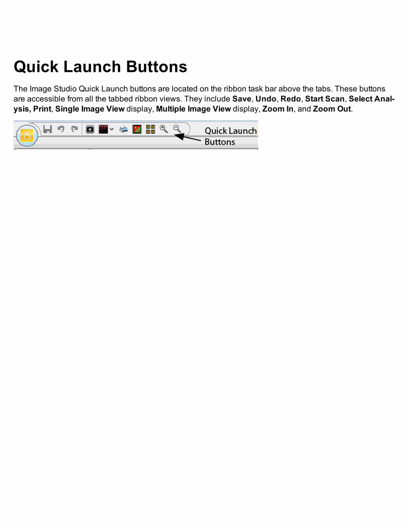
Quick Launch ButtonsThe Image Studio Quick Launch buttons are located on the ribbon task bar above the tabs. These buttonsare accessible from all the tabbed ribbon views. They include Save, Undo, Redo, Start Scan, Select Anal-ysis, Print, Single Image View display,Multiple Image View display, Zoom In, and Zoom Out.

Image LUTs (Lookup Table Values)The Lookup Table Panel or LUT Panel allows you to edit the parameters that display the selected image inthe image view. The LUT panel has individual panels for each channel available on a given acquisition.This example shows the 700 channel in red and the 800 channel in green. The x-axis of each panel rep-resents the raw pixel values. Each panel has a bar graph displaying a histogram of number of pixels witheach raw value. The higher the bar at a given location on the x-axis, the more pixels that contain that par-ticular intensity value. This histogram is shaded with the color map in use for that channel. Also shown ineach panel is an adjustable curve that maps raw data to displayed data.
The LUT Panel has individual panels for each channel available on a given acquisition.
Overlaying each histogram is an adjustable curve that represents how the raw data maps to the displayeddata. Adjust any of the three dots on the line (Max, Min, or K Value) to optimize the displayed image.To viewthe numbers, hover the mouse over one of the three dots in the line. The Max and Min numbers are dis-played. The middle one also shows the K value, which is used to smoothly change between linear (K=0)
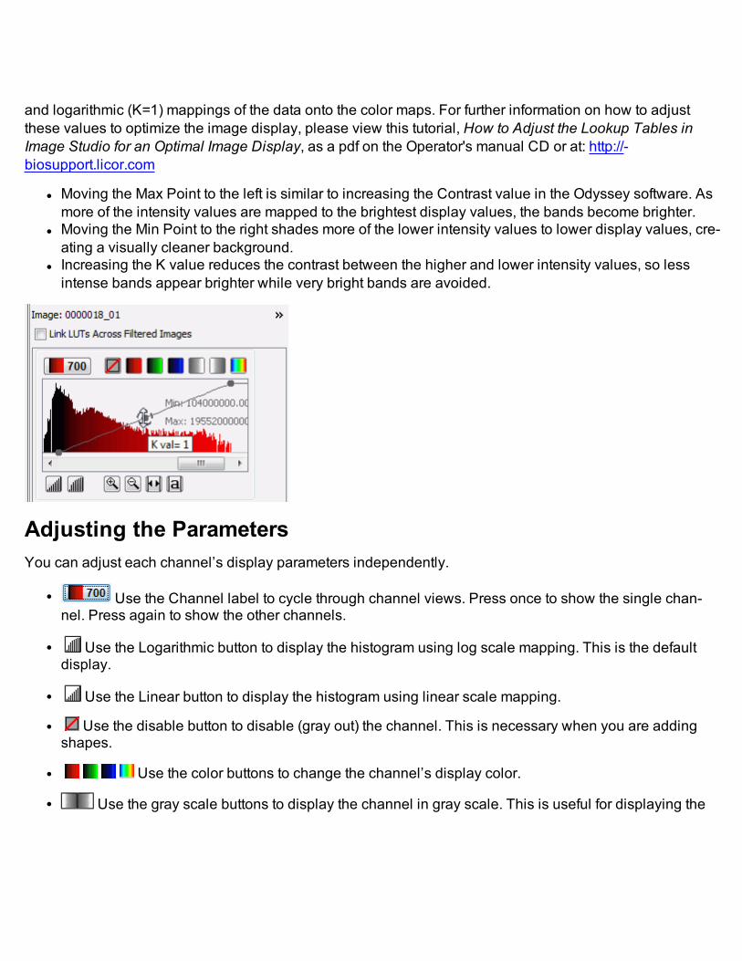
and logarithmic (K=1) mappings of the data onto the color maps. For further information on how to adjustthese values to optimize the image display, please view this tutorial, How to Adjust the Lookup Tables inImage Studio for an Optimal Image Display, as a pdf on the Operator's manual CD or at: http://-biosupport.licor.com
l Moving the Max Point to the left is similar to increasing the Contrast value in the Odyssey software. Asmore of the intensity values are mapped to the brightest display values, the bands become brighter.
l Moving the Min Point to the right shades more of the lower intensity values to lower display values, cre-ating a visually cleaner background.
l Increasing the K value reduces the contrast between the higher and lower intensity values, so lessintense bands appear brighter while very bright bands are avoided.
Adjusting the ParametersYou can adjust each channel’s display parameters independently.
l Use the Channel label to cycle through channel views. Press once to show the single chan-nel. Press again to show the other channels.
l Use the Logarithmic button to display the histogram using log scale mapping. This is the defaultdisplay.
l Use the Linear button to display the histogram using linear scale mapping.
l Use the disable button to disable (gray out) the channel. This is necessary when you are addingshapes.
l Use the color buttons to change the channel’s display color.
l Use the gray scale buttons to display the channel in gray scale. This is useful for displaying the
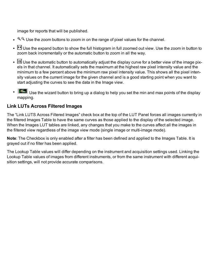
image for reports that will be published.
l Use the zoom buttons to zoom in on the range of pixel values for the channel.
l Use the expand button to show the full histogram in full zoomed out view. Use the zoom in button tozoom back incrementally or the automatic button to zoom in all the way.
l Use the automatic button to automatically adjust the display curve for a better view of the image pix-els in that channel. It automatically sets the maximum at the highest raw pixel intensity value and theminimum to a few percent above the minimum raw pixel intensity value. This shows all the pixel inten-sity values on the current image for the given channel and is a good starting point when you want tostart adjusting the curves to see the data in the Image view.
l Use the wizard button to bring up a dialog to help you set the min and max points of the displaymapping.
Link LUTs Across Filtered ImagesThe “Link LUTS Across Filtered Images” check box at the top of the LUT Panel forces all images currently inthe filtered Images Table to have the same curves as those applied to the display of the selected image.When the Images LUT tables are linked, any changes that you make to the curves affect all the images inthe filtered view regardless of the image view mode (single image or multi-image mode).
Note: The Checkbox is only enabled after a filter has been defined and applied to the Images Table. It isgrayed out if no filter has been applied.
The Lookup Table values will differ depending on the instrument and acquisition settings used. Linking theLookup Table values of images from different instruments, or from the same instrument with different acqui-sition settings, will not provide accurate comparisons.

ProfilesThe Profile tab on the right side of the application displays a lane, band, or shape profile. When only aband or shape is selected, the profile is displayed for just the band or shape. When a lane is selected, a laneprofile is shown that allows other options (e.g., Subtract Lane Background, etc.).
1. Select a single lane, band, or shape and click the Profiles tab. The profile panel is displayed.
2. You can modify the profile display by selecting one or both Channels (you must select at least one).
3. You can also choose whether to Subtract Lane Background and/or Display Lane Background.Note: These options are only available if you have selected a Lane Background method. Otherwise,these options are grayed out.
In this example, one band is selected, both channels are displayed, and background is subtracted.

ConcentrationAssign features as Concentration Standards and the concentration of all other features on the image are cal-culated and displayed in the table. You can add concentration standards to any analysis.
1. Click the first button on the Table ribbon. From the drop-down menu, select the table with the featuresthat you will assign as Concentration Standards.
2. Click Add/Remove in the Columns section.
3. Check the boxes next to Conc. Std. and Concentration to add these columns to the table. ClickSave.
4. Click a feature to highlight the row in the table. Note: Concentration standards can only be added toone channel at a time. Check that the highlighted row is in the correct channel.
5. Double-click the Conc. Std. field in the row.
6. Type a number in this field to order the concentration standards. Note: The values of the standards

must increase as the order increases.
7. Click the Concentration tab on the right side of the application window. The assigned concentrationstandard should appear in the list.
8. Repeat steps 4 through 6 to add all of the concentration standards to the list.
9. The calculated concentrations for the other features appear in the table in the Concentration column.

PreferencesThe Preferences dialog has choices for specifying general application features and for selecting the defaultimage display colors for new acquisitions. To display the Preferences dialog:
1. Click the Application menu button to display the menu.
2. Click the Preferences button in the Footer of the menu. The Preferences dialog is opened with theGeneral Preferences page displayed.
General PreferencesUse the General preferences to control general application features. You can set the undo limit, choosewhether to show tooltips, specify your organization name and company logo to display on imported images,
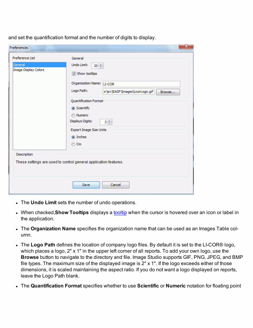
and set the quantification format and the number of digits to display.
l The Undo Limit sets the number of undo operations.
l When checked,Show Tooltips displays a tooltip when the cursor is hovered over an icon or label inthe application.
l The Organization Name specifies the organization name that can be used as an Images Table col-umn.
l The Logo Path defines the location of company logo files. By default it is set to the LI-COR® logo,which places a logo, 2" x 1" in the upper left corner of all reports. To add your own logo, use theBrowse button to navigate to the directory and file. Image Studio supports GIF, PNG, JPEG, and BMPfile types. The maximum size of the displayed image is 2" x 1". If the logo exceeds either of thosedimensions, it is scaled maintaining the aspect ratio. If you do not want a logo displayed on reports,leave the Logo Path blank.
l The Quantification Format specifies whether to use Scientific or Numeric notation for floating point

values. Note: Excel reports numeric formats using its default format for floating point fields. Thesefields my be displayed as both standard and scientific formats unless the formatting is overridden inExcel.
l Use the counter to specify the number of significant digits to display.
l The Export Image Size Units sets the size units to Inches or Centimeters.
Image Display Colors PreferencesClick the Image Display Colors choice in the Preference List. Use these preferences to specify the defaultimage display colors for new acquisitions.

TooltipsAll the buttons and group names on the ribbon have tooltips. To display the tooltip for a particular tab or com-mand, simply hover the mouse over the item and an explanation is displayed in a small window. This exam-ple shows the tooltip for the View Mode group.
Note: Make sure that you have "Show Tooltips" checked in the General Preferences dialog.

Work AreaA Work Area is a folder that contains the Settings, Logs, and Images files from Image Studio. This folder canbe located on a hard drive or network drive. All changes to the Settings are saved in the Work Area and willbe applied the next time the Work Area is opened in Image Studio.
Choose an Available Work Area1. Open the Image Studio software by double-clicking the desktop icon. The Set Active Work Areamenu
opens.
2. Choose an available Work Area for this session of Image Studio and click OK. You can also create anew Work Area.
Create a New Work AreaThe default Settings are applied in a new Work Area.
1. Click Browse... in the Set Active Work Area menu (see above).
2. Open the folder for the new Work Area. Click the New Folder button and name the new folder. This is

the new Work Area.
Transfer Images to a New Work AreaImages can be Exported from a Work Area and Imported into a Work Area.
See Copy Images for more information on copying images to a Backup Folder or a Zip File. To transferimages to a new Work Area, copy the images to a folder that was previously created as a Work Area.Another option is to copy the images to a Zip File and import them into a Work Area (see Import Images).
Images can also be moved from the Work Area to another folder (see Archive Images). The new folder canbe a previously created Work Area. Using the Move To (Archive) function deletes the images from the cur-rent Work Area.

Import ImagesYou can import acquisitions (images plus analysis data) from this application and images from the Odys-sey® Classic Imaging System, and the Pearl® Imager or the Pearl® Impulse.
1. Open the Application menu and choose Import to display the choices.
Copy FromCopy From copies an image folder or ZIP file from this application to the current default images folder. Theentire folder is copied, including images, analysis files, and other text files. This is useful if you have pre-viously transferred data to a different location for archiving or you are transferring data from another WorkArea.
1. Choose Copy From (Import Acquisition) from the Import submenu. The Import Acquisitions dialog isdisplayed.
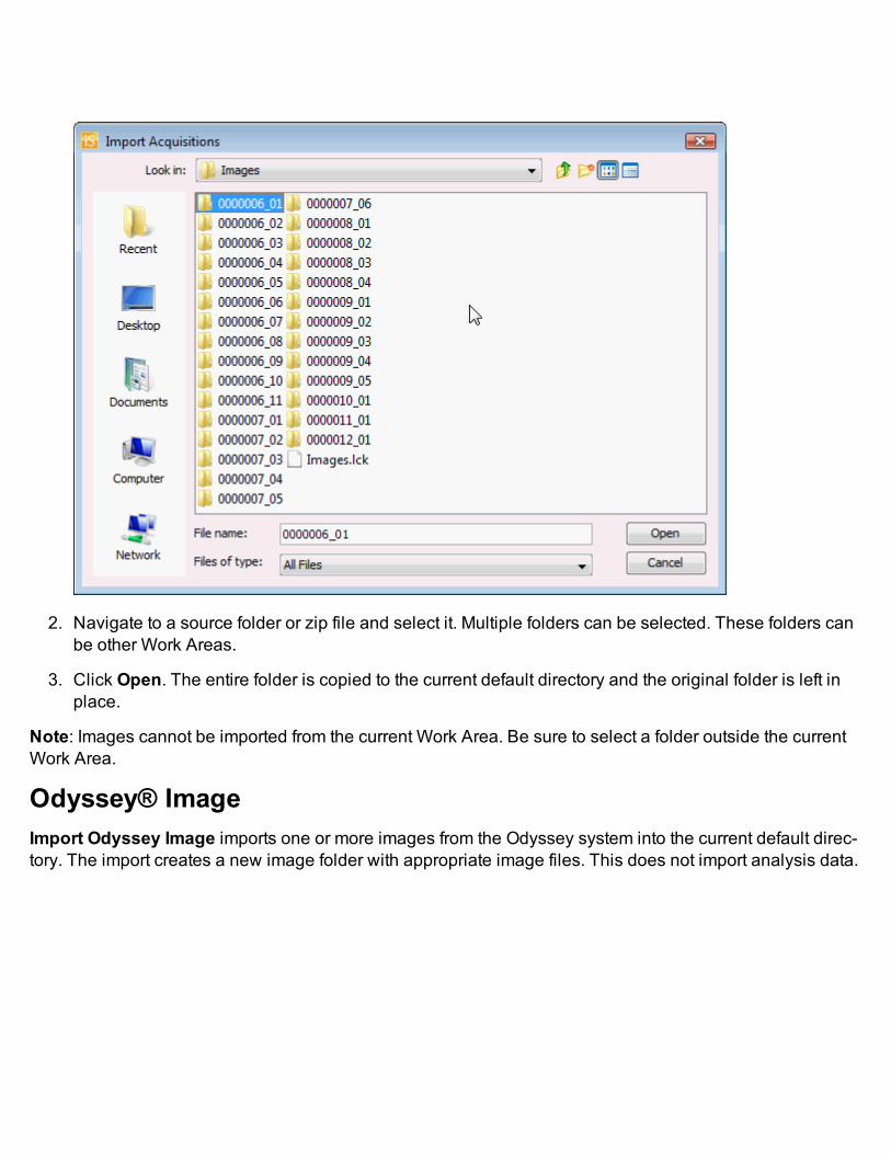
2. Navigate to a source folder or zip file and select it. Multiple folders can be selected. These folders canbe other Work Areas.
3. Click Open. The entire folder is copied to the current default directory and the original folder is left inplace.
Note: Images cannot be imported from the current Work Area. Be sure to select a folder outside the currentWork Area.
Odyssey® ImageImport Odyssey Image imports one or more images from the Odyssey system into the current default direc-tory. The import creates a new image folder with appropriate image files. This does not import analysis data.

1. Choose Odyssey Image from the Import submenu. The Import Odyssey Image(s) dialog is displayed.
2. Navigate to a source folder and select images to be imported into the default folder on the file system.
3. Select the image(s) to import and click Open. You can select one or more folders that contain severalTIF files from multiple channels. Note: The files need to be the same size and resolution.
You can also select a TIF file individually, or select two TIF files of the same image in different chan-nels. Note: Do not select multiple TIF files that are not of the same image.
4. The new TIF files are converted to a “float” format upon import. The original TIFs are not changed. The“Name” field inherits the Odyssey “acquisition Name” if a folder is imported. If only TIF files areimported, you are prompted for a “name.” The Image ID field for the new image is assigned a newunique Image ID.
Pearl® ImageImport Pearl Image imports one or more TIF files that were created in Pearl Cam Software.

1. Choose Pearl Image from the Import submenu. The Import Acquisition(s) dialog is displayed.
2. Navigate to a source folder and select images to be imported into the default folder on the file system.Click Open.
3. The “Name” field inherits the Pearl ImageID if a folder is imported. If only TIF files are imported, youare prompted for a “name." The Image ID field for the new image is the same as the imported ImageIDof the folder or Pearl Images.

Copy ImagesCopy Images copies the selected images and acquisitions from the Images Table to a folder or a zip file.When you copy the images, they are not removed from the Images Table.
1. Select the images that you want to Copy.
2. Open the Application menu.
3. Expand the Copy To menu from the Exportmenu and choose Backup Folder or Zip File. If youchoose Zip File the Zip File dialog is displayed.

4. Accept the default folder and zip filename or navigate to a folder where you want to save the copiedacquisitions.
5. Click Save when you have finished. The images and acquisitions are copied to a zip file in the loca-tion you specified.
If you choose Backup Folder the Backup Folder dialog is displayed.

6. Accept the default folder or navigate to a folder where you want to save the copied acquisitions.This folder could be a different Work Area that was previously created (see Work Area).
7. Click Save when you have finished. The images and acquisitions are copied to a folder in thelocation you specified.

Archive ImagesArchive Images moves the selected images and acquisitions from the Images Table to a folder for archiv-ing. (This folder could be a different Work Area.) When you archive the images, they are removed from theImages Table.
1. Select the images that you want to archive.
2. Open the Application menu.
3. Choose Move To (Archive) from the Exportmenu. A message is displayed.
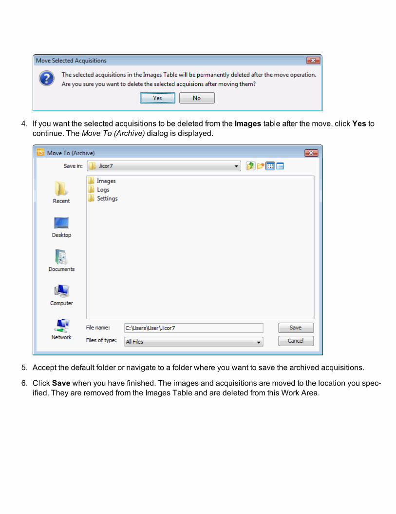
4. If you want the selected acquisitions to be deleted from the Images table after the move, click Yes tocontinue. The Move To (Archive) dialog is displayed.
5. Accept the default folder or navigate to a folder where you want to save the archived acquisitions.
6. Click Save when you have finished. The images and acquisitions are moved to the location you spec-ified. They are removed from the Images Table and are deleted from this Work Area.

Acquire TabThe Acquire tab contains controls for acquiring a new image. There is an Acquire tab specific for each typeof Instrument that is installed using its Import key (see Application menu for information about Import Keys).
l If only one Instrument key is installed, Image Studio will include that Acquire ribbon when the appli-cation is opened.
l If more than one Instrument key is installed, choose which Instrument type to use from the menu thatappears when opening Image Studio. To change to a different Instrument type, close Image Studio,open it again, and select a different Instrument type from the menu.
l If there is not an Instrument key installed or if you press Cancel instead of selecting an Instrument type,the Acquire Tab will not appear during that session.

Acquire Tab - Odyssey CLxThe Acquire tab contains controls for acquiring a new image on the Odyssey® CLx instrument.
SetupScan PresetUse the Scan Preset button in the Setup group to save the current settings as a scan preset, to select a pre-viously saved scan preset, or to delete a selected scan preset. A scan preset determines the Analysis Type,Channels to use, Channel Intensity settings, Resolution, Quality, and Scan Area settings.
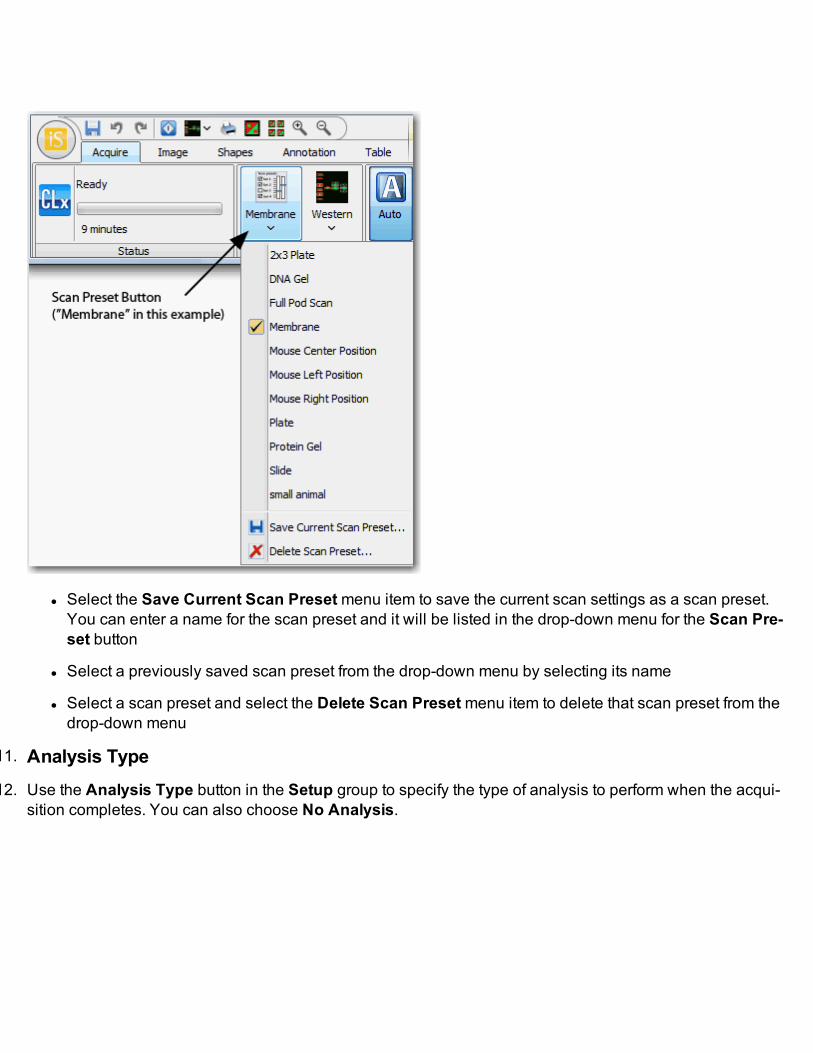
l Select the Save Current Scan Presetmenu item to save the current scan settings as a scan preset.You can enter a name for the scan preset and it will be listed in the drop-down menu for the Scan Pre-set button
l Select a previously saved scan preset from the drop-down menu by selecting its name
l Select a scan preset and select the Delete Scan Presetmenu item to delete that scan preset from thedrop-down menu
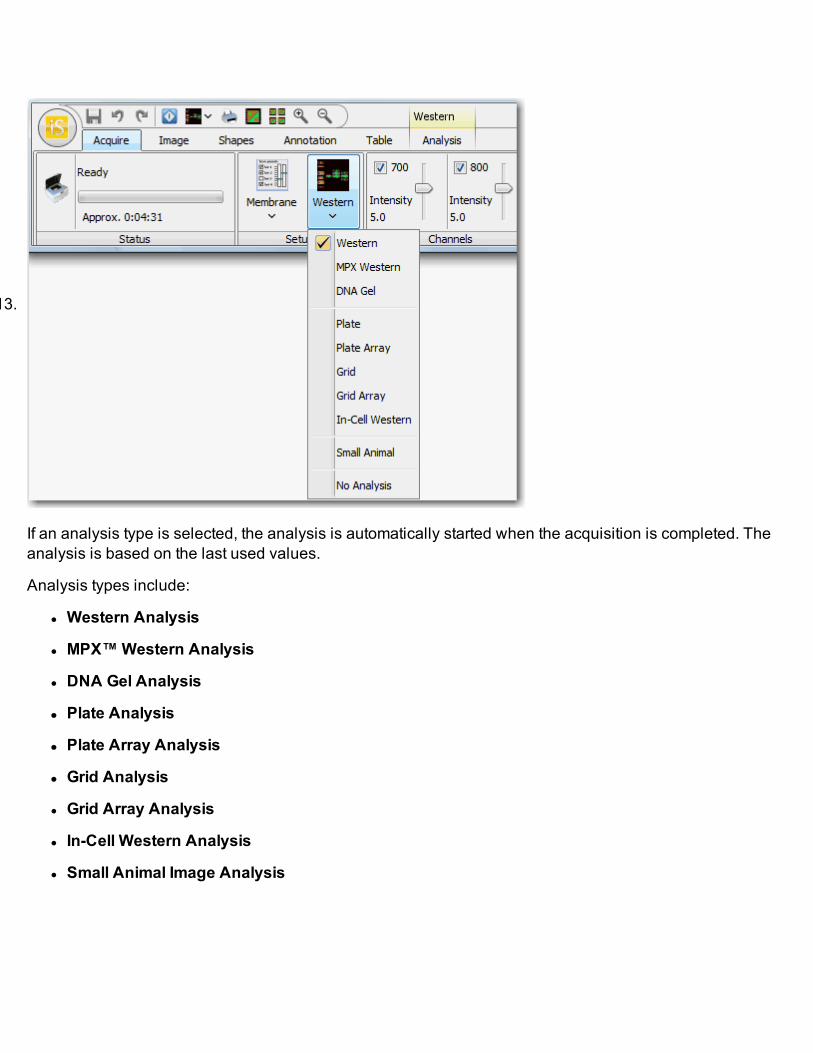
11. Analysis Type12. Use the Analysis Type button in the Setup group to specify the type of analysis to perform when the acqui-
sition completes. You can also choose No Analysis.

13.
If an analysis type is selected, the analysis is automatically started when the acquisition is completed. Theanalysis is based on the last used values.
Analysis types include:
l Western Analysis
l MPX™Western Analysis
l DNA Gel Analysis
l Plate Analysis
l Plate Array Analysis
l Grid Analysis
l Grid Array Analysis
l In-Cell Western Analysis
l Small Animal Image Analysis
Note: The Analysis Type choices may require the installation of separate Import Keys (see Applicationmenu for information about Import Keys).
No AnalysisTo analyze the data manually, select No Analysis from the drop-down menu. When the acquisition com-pletes, click on the Shapes tab to place Shapes on the areas of fluorescence and to define a background.You can also choose any of the other available analyses by clicking on the Analysis button on the Shapesribbon and selecting one from the drop-down menu.
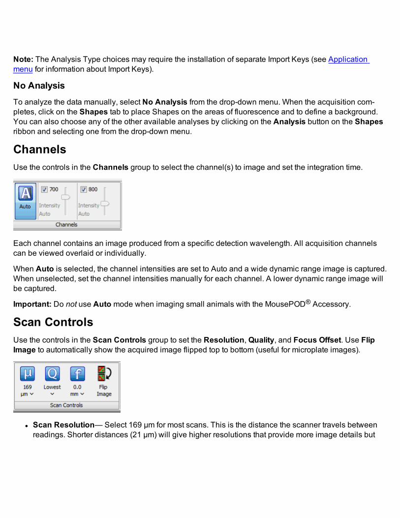
ChannelsUse the controls in the Channels group to select the channel(s) to image and set the integration time.
Each channel contains an image produced from a specific detection wavelength. All acquisition channelscan be viewed overlaid or individually.
When Auto is selected, the channel intensities are set to Auto and a wide dynamic range image is captured.When unselected, set the channel intensities manually for each channel. A lower dynamic range image willbe captured.
Important: Do not use Auto mode when imaging small animals with the MousePOD® Accessory.
Scan ControlsUse the controls in the Scan Controls group to set the Resolution,Quality, and Focus Offset. Use FlipImage to automatically show the acquired image flipped top to bottom (useful for microplate images).
l Scan Resolution— Select 169 µm for most scans. This is the distance the scanner travels betweenreadings. Shorter distances (21 µm) will give higher resolutions that provide more image details but
create large image files. Longer distances (337 µm) will give lower resolutions that provide smallimage files but do not offer fine image details.
l Scan Quality— Select the scan quality that affects the time and quality aspects of the scan. The low-est quality setting sets the fastest scan speed. Increasing the quality results in slower scan speeds, asmore detector readings are processed for a given area. The Lowest scan setting gives the fastest scantime and is appropriate for most scans.
l Focus Offset— Select the Focus Offset value from the list or enter a value by choosing the EnterValue menu item.
l Flip Image—When selected the image is automatically flipped top to bottom.
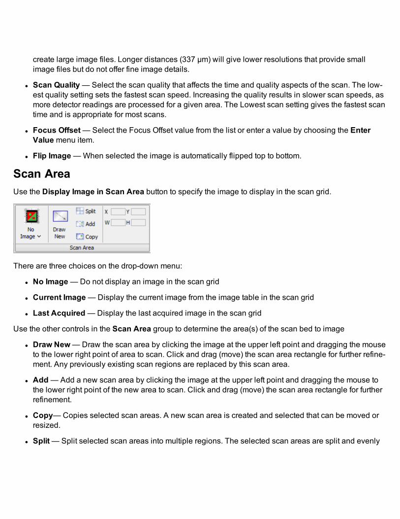
Scan AreaUse the Display Image in Scan Area button to specify the image to display in the scan grid.
There are three choices on the drop-down menu:
l No Image—Do not display an image in the scan grid
l Current Image—Display the current image from the image table in the scan grid
l Last Acquired—Display the last acquired image in the scan grid
Use the other controls in the Scan Area group to determine the area(s) of the scan bed to image
l Draw New—Draw the scan area by clicking the image at the upper left point and dragging the mouseto the lower right point of area to scan. Click and drag (move) the scan area rectangle for further refine-ment. Any previously existing scan regions are replaced by this scan area.
l Add— Add a new scan area by clicking the image at the upper left point and dragging the mouse tothe lower right point of the new area to scan. Click and drag (move) the scan area rectangle for furtherrefinement.
l Copy—Copies selected scan areas. A new scan area is created and selected that can be moved orresized.
l Split— Split selected scan areas into multiple regions. The selected scan areas are split and evenly

spaced in a row/column format. Multiple selected scan areas can optionally be merged into one areabefore splitting.
l Scan Area Location—Displays the X, Y, Width and Height controls for the selected scan area.TheAcquire Image View cursor location is also displayed.
ScannerUse the controls in the Scanner group to Start the scan. Use Preview to show the image as it is beingscanned.
l Start— Starts the image acquisition using the currently displayed parameter values. The status of theacquisition is displayed in the Status group. It also shows the channel being acquired, and the acqui-sition is listed in the Images Table.
l Preview—Creates a fast, low resolution preview image.
l Stop— Stops the current acquisition at the current point of collection.
l Cancel—Cancels the current acquisition. All existing and pending channel images are discarded.

Acquire Tab - Odyssey FcThe Acquire tab contains controls for acquiring a new image from theOdyssey® Fc instrument.
SetupSelect the type of analysis to perform when the acquisition completes. If an analysis type is selected, theanalysis is automatically started when the acquisition is completed. You can select:
l Western analysis— based on the last used values when the acquisition completes
l MPX™Western analysis— based on the last used values when the acquisition completes
l DNA analysis— based on the last used values when the acquisition completes
l None— do not perform any analysis when the acquisition completes
Note: The Analysis Type choices may require separate Import Keys (see Application menu for informationabout Import Keys).
ChannelsUse the controls in the Channels group to select the channels to include and position the slider to set theintegration time for each selected channel.

The acquisition times range from 30 seconds to 10 minutes, except for Chemi which ranges from 30 sec-onds to 60 minutes. Click on the arrow on the right side of the Channels bar to open a window and changethe sliders from standard to extended mode.
l In standard mode, only the 0.5, 2, and 10 minutes (and 60 minutes in Chemi) can be selected.
l In extended mode, the sliders can be adjusted to accommodate times in between. Use the arrow keysfor fine adjustment.
CameraClick the Acquire Image button in the Camera group to start the acquisition.
The image is acquired using the currently displayed parameter values. The status of the acquisition is dis-played in the Status group. It also shows the channel being acquired, and the acquisition is listed in theImages Table.
While the acquisition is collected, the images are displayed in the View area.
Note: To stop the acquisition before it has completed, press the Cancel button in the Camera group. Allexisting and pending channel images are discarded.

Acquire Tab - Odyssey ClassicThe Acquire tab contains controls for acquiring a new image on the Odyssey® Classic instrument.
SetupScan PresetUse the Scan Preset button in the Setup group to save the current settings as a scan preset, to select a pre-viously saved scan preset, or to delete a selected scan preset. A scan preset determines the Analysis Type,Channels to use, Channel Intensity settings, Resolution, Quality, and Scan Area settings.

l Select the Save Current Scan Presetmenu item to save the current scan settings as a scan preset.You can enter a name for the scan preset and it will be listed in the drop-down menu for the Scan Pre-set button.
l Select a previously saved scan preset from the drop-down menu by selecting its name.
l Select a scan preset and select the Delete Scan Presetmenu item to delete that scan preset from thedrop-down menu.
11. Analysis Type12. Use the Analysis Type button in the Setup group to specify the type of analysis to perform when the acqui-
sition completes. You can also choose No Analysis.
13.
If an analysis type is selected, the analysis is automatically started when the acquisition is completed. Theanalysis is based on the last used values.
Analysis types include:
l Western Analysis
l MPX™Western Analysis
l DNA Gel Analysis
l Plate Analysis
l Plate Array Analysis
l Grid Analysis
l Grid Array Analysis
l In-Cell Western Analysis
l Small Animal Image Analysis

Note: The Analysis Type choices may require the installation of separate Import Keys (see Applicationmenu for information about Import Keys).
No AnalysisTo analyze the data manually, select No Analysis from the drop-down menu. When the acquisition com-pletes, click on the Shapes tab to place Shapes on the areas of fluorescence and to define a background.You can also choose any of the other available analyses by clicking on the Analysis button on the Shapesribbon and selecting one from the drop-down menu.
ChannelsUse the controls in the Channels group to select the channels.
Each channel contains an image produced from a specific detection wavelength. All acquisition channelscan be viewed overlaid or individually.
Scan ControlsUse the controls in the Scan Controls group to set the Resolution,Quality, and Focus Offset. Use FlipImage to automatically show the acquired image flipped top to bottom (useful for microplate images).
l Scan Resolution— Select 169 µm for most scans. This is the distance the scanner travels betweenreadings. Shorter distances (21 µm) will give higher resolutions that provide more image details butcreate large image files. Longer distances (337 µm) will give lower resolutions that provide smallimage files but do not offer fine image details.
l Scan Quality— Select the scan quality that affects the time and quality aspects of the scan. The low-est quality setting sets the fastest scan speed. Increasing the quality results in slower scan speeds, asmore detector readings are processed for a given area. The Lowest scan setting gives the fastest scan
time and is appropriate for most scans.
l Focus Offset— Select the Focus Offset value from the list or enter a value by choosing the EnterValue menu item.
l Flip Image—When selected the image is automatically flipped top to bottom.
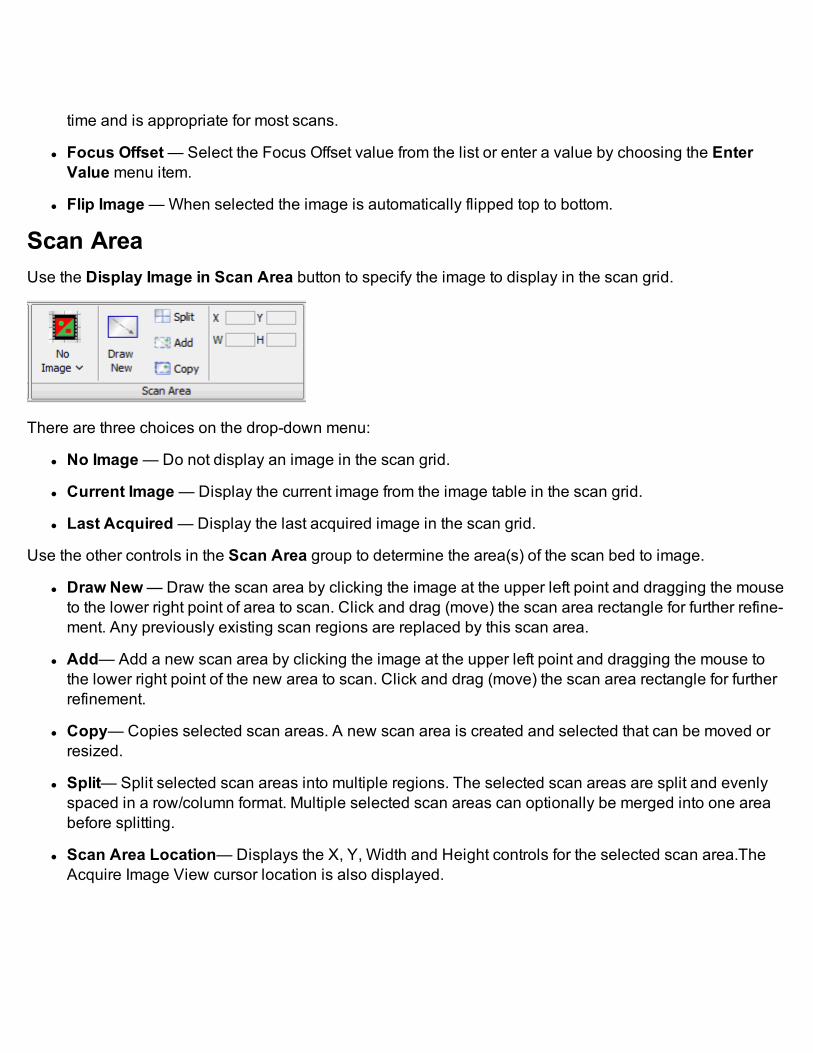
Scan AreaUse the Display Image in Scan Area button to specify the image to display in the scan grid.
There are three choices on the drop-down menu:
l No Image—Do not display an image in the scan grid.
l Current Image—Display the current image from the image table in the scan grid.
l Last Acquired—Display the last acquired image in the scan grid.
Use the other controls in the Scan Area group to determine the area(s) of the scan bed to image.
l Draw New—Draw the scan area by clicking the image at the upper left point and dragging the mouseto the lower right point of area to scan. Click and drag (move) the scan area rectangle for further refine-ment. Any previously existing scan regions are replaced by this scan area.
l Add— Add a new scan area by clicking the image at the upper left point and dragging the mouse tothe lower right point of the new area to scan. Click and drag (move) the scan area rectangle for furtherrefinement.
l Copy—Copies selected scan areas. A new scan area is created and selected that can be moved orresized.
l Split— Split selected scan areas into multiple regions. The selected scan areas are split and evenlyspaced in a row/column format. Multiple selected scan areas can optionally be merged into one areabefore splitting.
l Scan Area Location—Displays the X, Y, Width and Height controls for the selected scan area.TheAcquire Image View cursor location is also displayed.

ScannerUse the controls in the Scanner group to Start the scan. Use Preview to show the image as it is beingscanned.
l Start— Starts the image acquisition using the currently displayed parameter values. The status of theacquisition is displayed in the Status group. It also shows the channel being acquired, and the acqui-sition is listed in the Images Table.
l Preview—Creates a fast, low resolution preview image.
l Stop— Stops the current acquisition at the current point of collection.
l Cancel—Cancels the current acquisition. All existing and pending channel images are discarded.

Image TabThe Image tab has controls for zooming, viewing, copying, rotating or flipping, reducing noise, aligning chan-nels, and cropping an image. Selecting any of the options in the Create group creates a new image. Anyanalysis of the image is not copied. You can also display the Properties for the selected image.
DisplayUse the Image Adjust Assistant to adjust how the current image is displayed. Select a channel to adjust andthe current image is displayed in that channel, along with brighter and dimmer options. Adjust the signal,background, or midtones. Adjust the midtones to change the mapping from linear to logarithmic. This 'com-pression' of the intensity values may improve the appearance of less intense bands while avoiding overlybright bands.
ZoomThere are several zoom controls for zooming the image on the current analysis:
l Zoom In— Zooms in on the image. The zoom view is centered on the current pointer position on theimage. Press Zoom In again to zoom in another increment.
l Zoom Out— Zooms out on the image. Press Zoom Out again to zoom back out another increment.
l Zoom Selection— Zooms to the highest zoom that will display all selected features so that all the fea-tures are visible.
l Restore—Restores the zoom to fit the window.
l Zoom by %— Selects a zoom value for the current image view.
Note: Adjusting the mouse wheel over the image will also zoom in or zoom out.

View ModeThe View Mode lets you specify which view mode to use for displaying images. Select either the editableSingle Image Viewmode or the Multi-image Viewmode to display images in the main application window.Adjust display parameters for these images using the LUT Panels (see Lookup Table Values (LUTs) fordetails.)
l Single— Shows a single image that is fully editable. Any image in the Images Table can be displayedin an image view.
l Multiple— Shows several images from the Images Table. If there are a large number of images in theImages Table, only a subset of the images may be displayed. No edits can be made directly on theseviews. Use the drop-down menu to choose how many images to display horizontally.

Copy ImageCopy Image makes a copy of the original image (without the analysis) and gives it a new name. You will geta message that tells you that the copy was successful and the name of the new image.
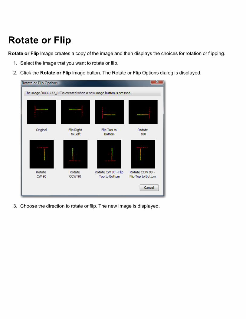
Rotate or FlipRotate or Flip Image creates a copy of the image and then displays the choices for rotation or flipping.
1. Select the image that you want to rotate or flip.
2. Click the Rotate or Flip Image button. The Rotate or Flip Options dialog is displayed.
3. Choose the direction to rotate or flip. The new image is displayed.
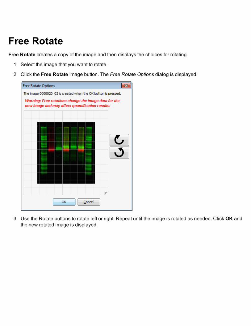
Free RotateFree Rotate creates a copy of the image and then displays the choices for rotating.
1. Select the image that you want to rotate.
2. Click the Free Rotate Image button. The Free Rotate Options dialog is displayed.
3. Use the Rotate buttons to rotate left or right. Repeat until the image is rotated as needed. Click OK andthe new rotated image is displayed.

Reduce NoiseReduce Noise creates a new image and reduces the noise on that image.
1. Select the Image.
2. Click the Reduce Noise button. The Reduce Noise Options dialog is displayed.
Choose one of the options defined below.
Noise Removal—Removes salt & pepper noise using a median filter
Smooth— Enhances the image using the local average
Local Maximum— Enhances the image using the local maximum
Sharpen— Enhances contrast at image boundaries
Local Minimum— Enhances the image using the local minimum
3. Click OK. A new image is created and noise on the new image is reduced.
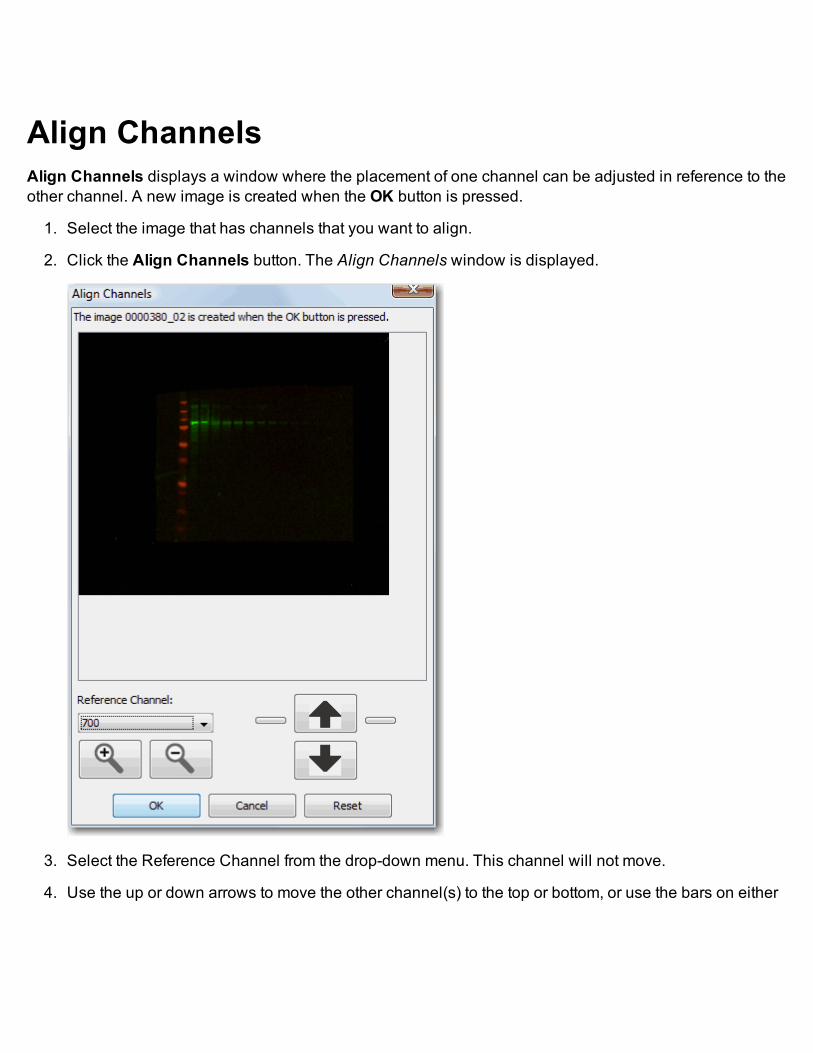
Align ChannelsAlign Channels displays a window where the placement of one channel can be adjusted in reference to theother channel. A new image is created when the OK button is pressed.
1. Select the image that has channels that you want to align.
2. Click the Align Channels button. The Align Channels window is displayed.
3. Select the Reference Channel from the drop-down menu. This channel will not move.
4. Use the up or down arrows to move the other channel(s) to the top or bottom, or use the bars on either

side of the arrows to move the other channel(s) left or right.
5. Click OK. A new image is created with the channels aligned.

CropThe Crop tools are for defining an area of display for exporting and printing as well as for cropping. Definingthe area for display doesn't crop the image but displays only the defined area when exporting and printingsingle images.
You can also crop an image using the defined area. A new image of the cropped area is created. The orig-inal image remains unchanged.
Define the Crop AreaThis action is used to define an area to display when exporting or printing an image for publication.
1. Display the image that you want to define.
2. Click the Modify button in the Crop Marks group. The crop area is outlined in a dotted line with a boxon each corner and a box in the center. The Edit Image Crop Marks dialog is also displayed. You mayneed to move the dialog if it is blocking the view of the crop area. (Note: You can change the color ofthe crop outline while it is selected by opening the Annotation tab and selecting a more contrastingcolor if the crop outline is hard to see on the image. Leave the Edit Image Crop Marks dialog open dur-ing this process.)


l Click the box in the center to move the entire crop area by using the four-pointed arrow to drag itto the area you want cropped.
l Click one of the boxes in a corner to resize the crop area by dragging the double arrow (up ordown or right or left).
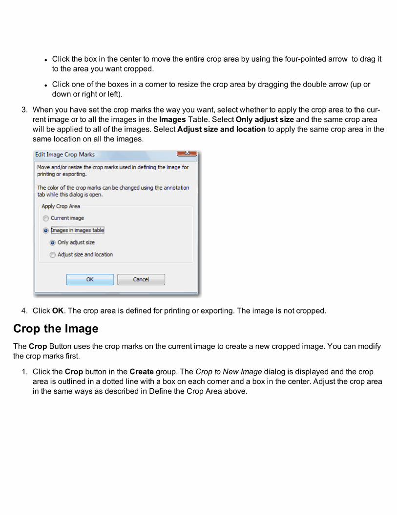
3. When you have set the crop marks the way you want, select whether to apply the crop area to the cur-rent image or to all the images in the Images Table. SelectOnly adjust size and the same crop areawill be applied to all of the images. Select Adjust size and location to apply the same crop area in thesame location on all the images.
4. Click OK. The crop area is defined for printing or exporting. The image is not cropped.
Crop the ImageThe Crop Button uses the crop marks on the current image to create a new cropped image. You can modifythe crop marks first.
1. Click the Crop button in the Create group. The Crop to New Image dialog is displayed and the croparea is outlined in a dotted line with a box on each corner and a box in the center. Adjust the crop areain the same ways as described in Define the Crop Area above.

2. Click OK. A new image of the cropped area is created.

Shapes TabThe Shapes tab is used to create a general analysis for any image.
l The Analysis group has a drop-down menu for specialized types of analysis. Select the type of anal-ysis to apply and the Analysis tab for that application is opened. The last used parameters for that par-ticular analysis type are used to create the new analysis.
l The Create group has tools for adding basic shapes to the image. These tools are not available inmulti-image mode. To use the Create tools, change the view to single image mode.
l The Edit group has tools for editing the shapes.
l The Background group has tools for defining the background.
l The Show options determine what is displayed on the image.

Adding ShapesShapes can be a rectangle, ellipse, or other shape drawn around some section of the image. Shapes can bequantified.
To add a shape:
1. Open the Analyze ribbon and choose the type of shape you want to add. There are several ways toplace a shape on the image:
l Add Rectangle—Click the center of the feature in the image view. The rectangle auto-matically surrounds the feature.
l Add Ellipse—Click the center of the feature in the image view. The ellipse automaticallysurrounds the feature.
Note: You can only add the auto shapes (Add Rectangle and Add Ellipse) to a single channelat a time. All other shapes will be added to all channels that are currently visible.
l Add Selection— Select a shape. Click the center of the feature in the image view whereyou want to add a shape. The selected shape is copied and added.
l Draw Rectangle—Click and drag from the top left to the bottom right to surround the fea-ture.
l Draw Ellipse—Click the center of the feature and drag to the right or left to surround it.
l Draw Freehand—Click and drag the shape until it surrounds the area of interest.
2. Continue adding the selected shape until you have finished.
3. Click the Select button to end adding shapes (or press the ESC key on your keyboard).

Editing ToolsThere are several tools for editing features on an image. To edit one or more features, first select the fea-ture(s).
Selecting a feature1. Click the Select icon .
2. Click anywhere inside the feature that you want to select.
3. To extend the selection (select another feature), hold down the CTRL key and click anywhere insidethe next feature you want to select.
Note: You can also do a "sweep" selection by drawing a box around a set of shapes. Add to the selectionsusing the CTRL key.
Select AllClick Select All to select all features on the image. Selection will include all shapes, labels, and any anno-tation you may have added.
Deselect AllClick Deselect All to deselect all selected features on the image (or click the image anywhere outside theselected features).
Invert SelectionSelect a feature, then click Invert Selection to deselect the feature you selected and select everything elseon the image.
CutSelect the feature (or features) that you want to cut, then click Cut.
CopySelect the feature (or features) that you want to copy, then click Copy.
PastePlace the cursor where you want to place the copied or cut feature (or features), then click Paste.
DeleteSelect the feature (or features) that you want to delete, then click Delete.
Duplicate Across ChannelsSelect the feature(s) that you want to duplicate on other channels, then click Duplicate. This copies theselected features on one channel and pastes them on all other channels.
RotateSelect the feature that you want to rotate, then click Rotate.

BackgroundUse the controls in the Background group to specify the type of background.
1. Click the Set Background Type button. Select the Background Method from the drop-down menu.
l None—Do not subtract a background value
l Average.. .— Average of pixel values in the selected background segments
l Median...—Median of pixel values in the selected background segments
l User-Defined—Use a region to determine the background (the region is defined by a shapeyou select and then assign by clicking the Assign Shape button).
2. Selecting Average... orMedian... opens the Background dialog.
Select the segments around the band to use as background.
l All—Use all boundary segments for average or median background subtraction.
l Top/Bottom—Use top/bottom segments for average or median background subtraction.
l Right/Left—Use right/left segments for average or median background subtraction.
Use the Border width drop-down menu to specify the width of the background border in pixels.
3. Click Save when you have finished.
Note: To visualize the pixels that are used for backgrounds using the Average and Median methods, use theShow Local Background setting.


Show Groupl Shapes— Shows the shapes on image view. Exports and prints of the image view will show shapeswhen this Show option is checked.
l Labels— Shows labels of features on the image. Exports and prints of the image view will showlabels when this Show option is checked.
1. To specify where to place the labels, click the arrow at the bottom right of the Show group.
This opens the Image View Labels dialog.
2. Use the drop-down menus to select the position for the labels and what quantification value todisplay if Quantification is checked.
3. Click OK when you have finished.
l Quantification— A quantification value can be displayed on the image. Select from the drop-downmenu in the Image View Labels dialog shown above.
l Local Background— Show local (Average or Median) background area used for shapes in the

Image View.
l Text— Shows any text that you may have added on an image. Exports and prints of the image viewwill show text when this Show option is checked.
l Color Bar— Show a color bar on the single image view when only one channel is showing. The colorbar is also shown on exports and prints of the image view.
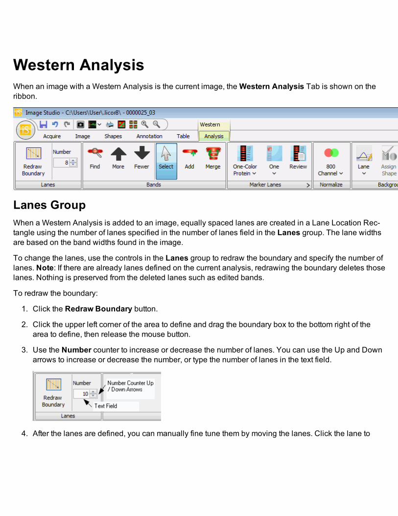
Western AnalysisWhen an image with a Western Analysis is the current image, theWestern Analysis Tab is shown on theribbon.
Lanes GroupWhen a Western Analysis is added to an image, equally spaced lanes are created in a Lane Location Rec-tangle using the number of lanes specified in the number of lanes field in the Lanes group. The lane widthsare based on the band widths found in the image.
To change the lanes, use the controls in the Lanes group to redraw the boundary and specify the number oflanes. Note: If there are already lanes defined on the current analysis, redrawing the boundary deletes thoselanes. Nothing is preserved from the deleted lanes such as edited bands.
To redraw the boundary:
1. Click the Redraw Boundary button.
2. Click the upper left corner of the area to define and drag the boundary box to the bottom right of thearea to define, then release the mouse button.
3. Use the Number counter to increase or decrease the number of lanes. You can use the Up and Downarrows to increase or decrease the number, or type the number of lanes in the text field.
4. After the lanes are defined, you can manually fine tune them by moving the lanes. Click the lane to

select it, then drag the top or the bottom to tilt it or hold down the shift key to move the whole lane left orright to a new position. To select more than one lane to move or tilt, hold down the CTRL key whileclicking (selecting) the lanes. Move the cursor to the top or bottom of the lane and when the cursorturns to the four-pointed arrow, drag it left or right to tilt the group; or hold down the SHIFT key, drag thecursor left or right to move the group.
(Note: During the Find Bands process, the lanes are also adjusted to optimize their intersection withthe bands.)

Note: After band finding is complete, if you move or resize a lane, the band-finding process is repeatedusing the same parameters.
Bands GroupUse the controls in the Bands group to Find bands, to adjust the band finding parameters to find More orFewer bands, to Add Bands, and Merge Bands.
To find bands:
1. Click the Find Bands button.
2. Review the results. If there are too many bands, click the Fewer arrow; if there are too few bands, clickthe More arrow. Repeat if necessary. The button is grayed out when the More and Fewer controlshave reached their respective upper or lower end of the band sensitivity range.
3. If a band is shown as several bands instead of a single band, select the bands and click the Merge but-ton.
4. To insert a band into a lane, click the Add button at the point on a lane you want the band added. Thewidth of the band is the width of the current lane.
Marker GroupUse the controls in the Marker group to select the Marker set to use, to specify the number of markers, and toadd new markers or delete selected markers.
When you initially define sizing for an analysis, the number of marker lanes are assigned from the left-mostlane, continuing to lanes to the right. In this example, two marker lanes are assigned. They are labeled M1and M2.

The sizes defined in the marker lane set are assigned to the bands in the marker lanes from top to bottom.
Sizing information is displayed in the Bands Table using "Size" column. For bands in the Marker Lanes, thesizes are the standards sizes; for all other bands, the sizes are calculated. See Bands Table for more infor-mation.

Reviewing a Marker1. Click the Markers button to display the list of Markers.
2. Select the marker that you want to review.
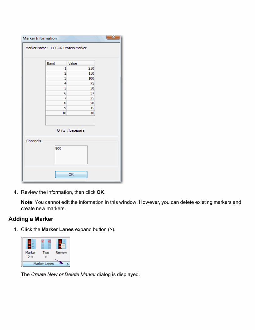
3. Click the Review button. The Marker Information dialog is displayed.

4. Review the information, then click OK.
Note: You cannot edit the information in this window. However, you can delete existing markers andcreate new markers.
Adding a Marker1. Click the Marker Lanes expand button (>).
The Create New or Delete Marker dialog is displayed.
2. Click the New button. The Name Marker dialog is displayed.
3. Enter a new Marker name in the text field and click OK. The New Marker dialog is displayed.
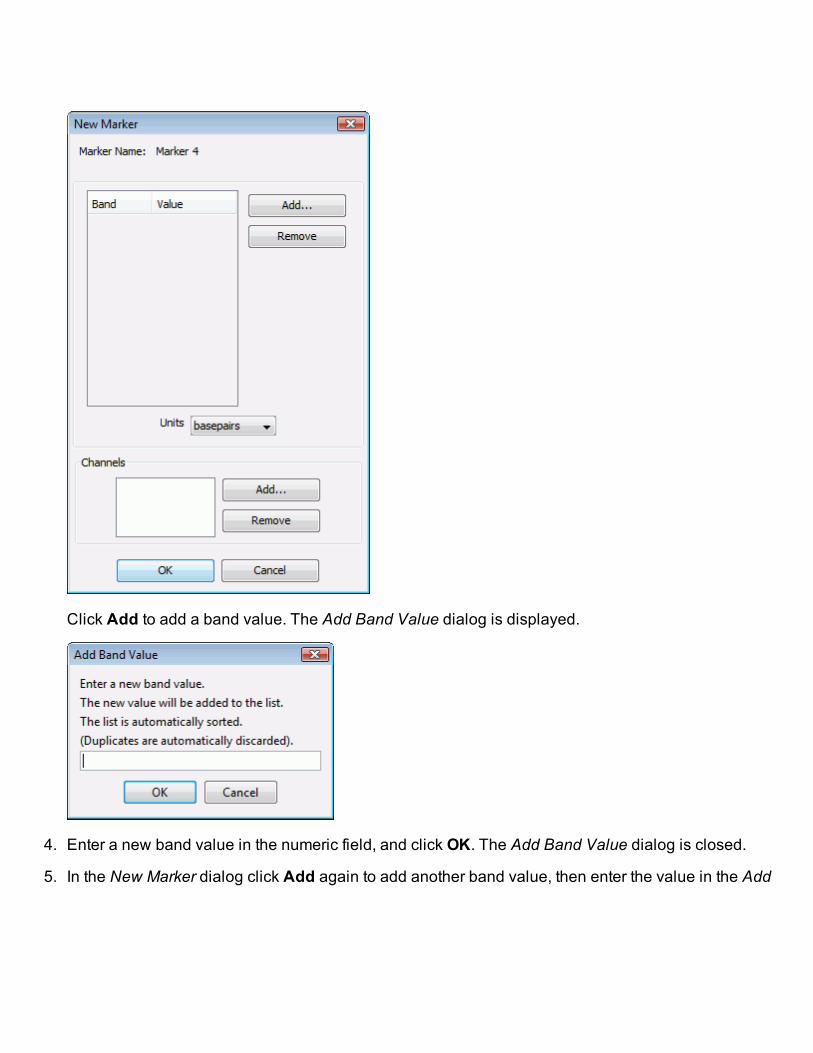
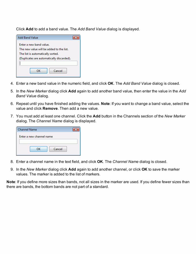
Click Add to add a band value. The Add Band Value dialog is displayed.
4. Enter a new band value in the numeric field, and click OK. The Add Band Value dialog is closed.
5. In the New Marker dialog click Add again to add another band value, then enter the value in the Add

Band Value dialog.
6. Repeat until you have finished adding the values. Note: If you want to change a band value, select thevalue and click Remove. Then add a new value.
7. You must add at least one channel. Click the Add button in the Channels section of the New Markerdialog. The Channel Name dialog is displayed.
8. Enter a channel name in the text field, and click OK. The Channel Name dialog is closed.
9. In the New Marker dialog click Add again to add another channel, or click OK to save the markervalues. The marker is added to the list of markers.
Note: If you define more sizes than bands, not all sizes in the marker are used. If you define fewer sizes thanthere are bands, the bottom bands are not part of a standard.
Deleting a Marker1. Click the Markers button to display the list of Markers
Select the marker that you want to delete.
2. Click the Marker Lanes expand button (>).

The Create New or Delete Marker dialog is displayed.
3. Click the Delete button. You are prompted to confirm deletion. Click Yes to delete the marker or clickNo if you changed your mind.
Note: The deleted marker will still appear on other images where it was used previously. An asteriskwill appear after the marker's name to designate that it is a deleted marker.
Normalize GroupUse the Normalize group to specify the normalization Channel to use for band normalization. Normalizationis useful for using one channel to correct for loading variation between lanes. (See Band Normalization formore information.)
1. Click the Channels button in the Normalize group to display the channels.
2. Select the channel to use for band normalization.
Background GroupUse the controls in the Background group to specify the type of background.

The Lane background is the recommended background method for Westerns. Note: Click a Lane to select itand click Profiles on the right side of the application window to see the lane background.
1. Select None, Average,Median, Lane, or User-Defined from the drop-down menu.
l None: Do not subtract a background value (band signal and other quantification values thatdepend on signal will have a value of NaN, meaning undefined)
l Average: Average of pixel values in the selected background segments
l Median: Median of pixel values in the selected background segments
l All: Use all boundary segments for average or median
l Top/Bottom: Use top/bottom segments for average or median
l Right/Left: Use right/left segments for average or median
l Lane: Subtract the background pixel values in the lane
l User-Defined: Assign a shape to determine the background (if region is undefined, band signaland other quantification values that depend on signal will have a value of NaN, meaning unde-fined)
2. For Average orMedian background, use the Background dialog to specify the width of the back-ground border in pixels.
3. Click Save when you have finished.
Show GroupUse the controls in the Show group to specify what to display on the image. You can display Bands, Lanes,Labels,Quantification, Boundary,Marker Handle, and Local Background (see Show Group for furtherdetails).

The check boxes are toggles. Click to check the box; click again to uncheck the box.

MPX Western AnalysisWhen an image with an MPX™Western Analysis is the current image, the MPX Western Analysis Tab isshown on the ribbon.
Comb GroupWhen an MPX Western Analysis is applied to an image, lanes are created in a Lane Location Rectangleusing the MPX comb selection.
To change the lanes, use the controls in the Comb group to redraw the boundary or change the comb selec-tion. Note: If there are already lanes defined on the current analysis, redrawing the boundary deletes thoselanes. Nothing is preserved from the deleted lanes such as lane position or edited bands.
To redraw the boundary:
1. Click the Redraw Boundary button.
2. Click the upper left corner of the area to define and drag the boundary box to the bottom right ofthe area to define, then release the mouse button.
3. After the lanes are defined, you can manually fine tune them by moving the lanes. Click the laneto select it, then drag the top or the bottom to tilt it or hold down the shift key to move the wholelane left or right to a new position. To select more than one lane to move or tilt, hold down theCTRL key while clicking (selecting) the lanes. Move the cursor to the top or bottom of the laneand when the cursor turns to the four-pointed arrow, drag it left or right to tilt the group; or holddown the SHIFT key, drag the cursor left or right to move the group.
(Note: the Find Bands process also optimizes the lane location.)
Note: After band finding is complete, if you move or resize a lane, the band-finding process is repeatedusing the same parameters.

Bands GroupUse the controls in the Bands group to Find bands, to adjust the band-finding parameters to find More orFewer bands, to Add Bands, and toMerge Bands.
To find bands:
1. Click the Find Bands button.
2. Review the results. If there are too many bands, click the Fewer arrow; if there are too few bands,click the More arrow. Repeat if necessary. The button is grayed out when the More and Fewercontrols have reached their respective upper or lower end of the band sensitivity range.
3. If a band is shown as several bands instead of a single band, select the bands and click theMerge button.
4. To insert a band into a lane, click the Add button at the point on a lane you want the band added.The width of the band is the width of the current lane.
Marker GroupUse the controls in the Marker group to select the Marker set to use, to add new markers, or delete selectedmarkers.
The sizes defined in the marker lane set are assigned from the bands in the marker lanes from top to bottom.
Sizing information is displayed in the Bands Table using the "Size" column. See Bands Table for moreinformation.
Reviewing a Marker1. Click the Markers button to display the list of Markers.
2. Select the marker that you want to review.

3. Click the Review button. The Marker Information dialog is displayed.
4. Review the information, then click OK.
Note: You cannot edit the information in this window. However, you can delete existing markersand create new markers.
Adding a Marker1. Click the Marker Lanes expand button (>).
The Create New or Delete Marker dialog is displayed.

2. Click the New button. The Name Marker dialog is displayed.
3. Enter a new Marker name in the text field and click OK. The New Marker dialog is displayed.

Click Add to add a band value. The Add Band Value dialog is displayed.
4. Enter a new band value in the numeric field, and click OK. The Add Band Value dialog is closed.
5. In the New Marker dialog click Add again to add another band value, then enter the value in theAdd Band Value dialog.
6. Repeat until you have finished adding the values. Note: If you want to change a band value,select the value and click Remove. Then add a new value.
7. You must add at least one channel. Click the Add button in the Channels section of the NewMarker dialog. The Channel Name dialog is displayed.
8. Enter a channel name in the text field, and click OK. The Channel Name dialog is closed.
9. In the New Marker dialog click Add again to add another channel, or click OK to save the markervalues. The marker is added to the list of markers.
Note: If you define more sizes than bands, not all sizes in the marker are used. If you define fewer sizes thanthere are bands, the bottom bands are not part of a standard.

Deleting a Marker1. Click the Markers button to display the list of Markers
Select the marker that you want to delete.
2. Click the Marker Lanes expand button (>).
The Create New or Delete Marker dialog is displayed.
3. Click the Delete button. You are prompted to confirm deletion. Click Yes to delete the marker orclick No if you changed your mind.
Normalize GroupUse the Normalize group to specify the normalization Channel to use for band normalization. Normalizationis useful for using one channel to correct for loading variation between lanes. (See Band Normalization formore information.)

1. Click the Channels button in the Normalize group to display the channels.
2. Select the channel to use for band normalization.
Background GroupUse the controls in the Background group to specify the type of background. The Lane background is therecommended background method for MPX Westerns.
Note: Click a Lane to select it and click Profiles on the right side of the application window to see the lanebackground.
1. Select None, Average,Median, Lane, or User-Defined from the drop-down menu.
l None: Do not subtract a background value (band signal and other quantification values thatdepend on signal will have a value of NaN, meaning undefined)
l Average: Average of pixel values in the selected background segments
l Median: Median of pixel values in the selected background segments
l All: Use all boundary segments for average or median
l Top/Bottom: Use top/bottom segments for average or median
l Right/Left: Use right/left segments for average or median
l Lane: Subtract the background pixel values in the lane

l User-Defined: Assign a shape to determine the background (if region is undefined, band signaland other quantification values that depend on signal will have a value of NaN, meaning unde-fined)
2. For Average orMedian background, use the Background dialog to specify the width of the back-ground border in pixels.
3. Click Save when you have finished.
Show GroupUse the controls in the Show group to specify what to display on the image. You can display Bands, Lanes,Labels,Quantification,Boundary,Marker Handle, and Local Background (see Show Group for furtherdetails).
The check boxes are toggles. Click to check the box; click again to uncheck the box.

DNA Gel AnalysisWhen an image with a DNA Gel Analysis is the current image, the DNA Gel Analysis Tab is shown on theribbon.
Lanes GroupWhen a DNA Gel Analysis is added to an image, equally spaced lanes are created in a Lane Location Rec-tangle using the number of lanes specified in the number of lanes field in the Lanes group. The lane widthsare based on the band widths found in the image.
To change the lanes, use the controls in the Lanes group to redraw the boundary and/or to change thenumber of lanes. Note: If there are already lanes defined on the current analysis, redrawing the boundarydeletes those lanes. Nothing is preserved from the deleted lanes such as edited bands.
To redraw the boundary:
1. Click the Redraw Boundary button.
2. Click the upper left corner of the area to define and drag the boundary box to the bottom right of thearea to define, then release the mouse button.
3. Use the Number counter to increase or decrease the number of lanes. You can use the Up and Downarrows to increase or decrease the number, or type the number of lanes in the text field.
4. After the lanes are defined, you can manually fine tune them by moving the lanes. Click the lane to

select it, then drag the top or the bottom to tilt it or hold down the shift key to move the whole lane left orright to a new position. To select more than one lane to move or tilt, hold down the CTRL key whileclicking (selecting) the lanes. Move the cursor to the top or bottom of the lane and when the cursorturns to the four-pointed arrow, drag it left or right to tilt the group; or hold down the SHIFT key, drag thecursor left or right to move the group. (See illustration in the Lanes group section of Western Analysis.)
(Note: During the Find Bands process, the lanes are also adjusted to optimize their intersection with thebands.)
After band finding is complete, if you move or resize a lane, the band-finding process is repeated using thesame parameters.
Bands GroupUse the controls in the Bands group to Find bands, to adjust the band finding parameters to find More orFewer bands, to Add Bands, and toMerge Bands.
To find bands:
1. Click the Find Bands button.
2. Review the results. If there are too many bands, click the Fewer arrow; if there are too few bands, clickthe More arrow. Repeat if necessary. The button is grayed out when the More and Fewer controlshave reached their respective upper or lower end of the band sensitivity range.
3. If a band is shown as several bands instead of a single band, select the bands and click the Merge but-ton.
4. To insert a band into a lane, click the Add button at the point on a lane you want the band added. Thewidth of the band is the width of the current lane.
Marker GroupUse the controls in the Marker group to select the Marker set to use, to specify the number of markers, and toadd new markers or delete selected markers.
When you initially define sizing for an analysis, the number of marker lanes are assigned from the left-mostlane, continuing to lanes to the right.
The sizes defined in the marker lane set are assigned from the bands in the marker lanes from top to bottom.
Sizing information is displayed in the Bands Table using "Size" column. For bands in the Marker Lanes, thesizes are the standards sizes; for all other bands, the sizes are calculated. See Bands Table for more infor-mation.

Reviewing a Marker1. Click the Markers button to display the list of Markers.
2. Select the marker that you want to review.
3. Click the Review button. The Marker Information dialog is displayed.
4. Review the information, then click OK.
Note: You cannot edit the information in this window. However, you can delete existing markers andcreate new markers.
Adding a Marker1. Click the Marker Lanes expand button (>).
The Create New or Delete Marker dialog is displayed.

2. Click the New button. The Name Marker dialog is displayed.
3. Enter a new Marker name in the text field and click OK. The New Marker dialog is displayed.
Click Add to add a band value. The Add Band Value dialog is displayed.
4. Enter a new band value in the numeric field, and click OK. The Add Band Value dialog is closed.
5. In the New Marker dialog click Add again to add another band value, then enter the value in the AddBand Value dialog.
6. Repeat until you have finished adding the values. Note: If you want to change a band value, select thevalue and click Remove. Then add a new value.
7. You must add at least one channel. Click the Add button in the Channels section of the New Markerdialog. The Channel Name dialog is displayed.
8. Enter a channel name in the text field, and click OK. The Channel Name dialog is closed.
9. In the New Marker dialog click Add again to add another channel, or click OK to save the markervalues. The marker is added to the list of markers.
Note: If you define more sizes than bands, not all sizes in the marker are used. If you define fewer sizes thanthere are bands, the bottom bands are not part of a standard.

Deleting a Marker1. Click the Markers button to display the list of Markers
Select the marker that you want to delete.
2. Click the Marker Lanes expand button (>).
The Create New or Delete Marker dialog is displayed.
3. Click the Delete button. You are prompted to confirm deletion. Click Yes to delete the marker or clickNo if you changed your mind.
Note: The deleted marker will still appear on other images where it was used previously. An asteriskwill appear after the marker's name to designate that it is a deleted marker.

Background GroupUse the controls in the Background group to specify the type of background. The Lane background is therecommended background method for DNA gels.
Note: Click a Lane to select it and click Profiless on the right side of the application window to see the lanebackground.
1. Select None, Average,Median, Lane, or User-Defined from the drop-down menu.
l None: Do not subtract a background value (band signal and other quantification values thatdepend on signal will have a value of NaN, meaning undefined)
l Average: Average of pixel values in the selected background segments
l Median: Median of pixel values in the selected background segments
l All: Use all boundary segments for average or median
l Top/Bottom: Use top/bottom segments for average or median
l Right/Left: Use right/left segments for average or median
l Lane: Subtract the background pixel values in the lane
l User-Defined: Assign a shape to determine the background (if region is undefined, band signaland other quantification values that depend on signal will have a value of NaN, meaning unde-fined)
2. For Average orMedian background, use the Background dialog to specify the width of the back-ground border in pixels.
3. Click Save when you have finished.

Show GroupUse the controls in the Show group to specify what to display on the image. You can display Bands, Lanes,Labels,Quantification, Boundary,Marker Handle, and Local Background (see Show Group for furtherdetails).
The check boxes are toggles. Click to check the box; click again to uncheck the box.
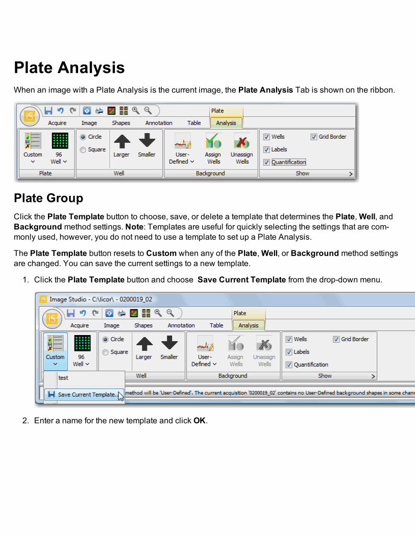
Plate AnalysisWhen an image with a Plate Analysis is the current image, the Plate Analysis Tab is shown on the ribbon.
Plate GroupClick the Plate Template button to choose, save, or delete a template that determines the Plate,Well, andBackground method settings. Note: Templates are useful for quickly selecting the settings that are com-monly used, however, you do not need to use a template to set up a Plate Analysis.
The Plate Template button resets to Custom when any of the Plate,Well, or Background method settingsare changed. You can save the current settings to a new template.
1. Click the Plate Template button and choose Save Current Template from the drop-down menu.
2. Enter a name for the new template and click OK.

3. Choose the type of plate from the Define Plate Type drop-down menu. You can choose from 6, 12, 24,48, 96, 384, or 1536 well configurations. If your plate does not fall into one of these types, selectGridAnalysis on the Shapes ribbon to set up a custom grid that fits your plate configuration.
4. Adjust the size of the plate by selecting the bounding box and dragging the green arrows on each side.Move the entire plate by dragging the double arrows that appear when hovering on the image.
Well GroupUse the Circle or Square buttons in theWell group to select the shape of the wells. Use the Larger orSmallerbuttons to incrementally adjust the size of the wells for a better fit.
Background GroupUse the controls in the Background group to specify the type of background.
You can choose None or User-Defined. If you select User-Defined, you will need to assign wells for thebackground.
1. Click the Background button and select User-Defined from the drop-down menu.
2. Select a well by clicking on the well. The selected well will have a dashed border. To select multiplewells, click and drag a bounding box around the wells or hold down the Ctrl key while clicking on eachwell.

3. Click Assign Wells and all selected wells will be assigned as background wells. Note: Any wells thatwere previously assigned as background wells are automatically unassigned.
4. To unassign any wells, select the well or wells (see step 2 above) and click Unassign Wells.
Show GroupUse the controls in the Show group to specify what to display on the image. You can displayWells, Labels,Quantification, and Grid Border (see Show Group for further details).
The check boxes are toggles. Click to check the box; click again to uncheck the box.
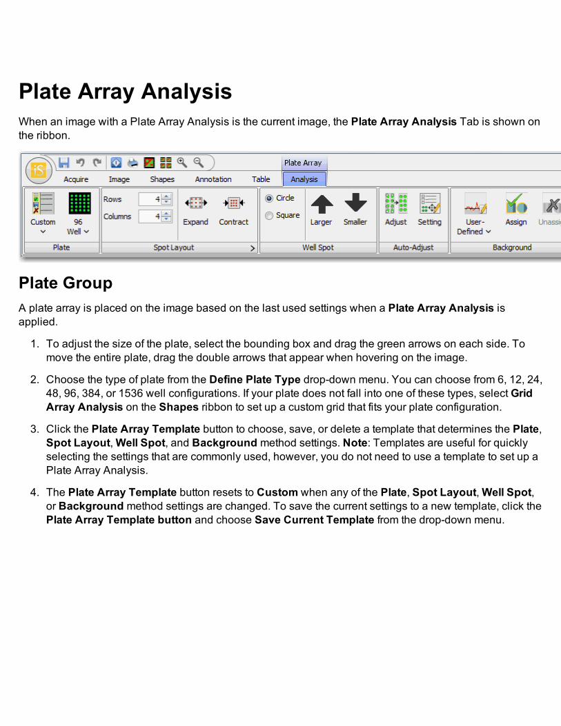
Plate Array AnalysisWhen an image with a Plate Array Analysis is the current image, the Plate Array Analysis Tab is shown onthe ribbon.
Plate GroupA plate array is placed on the image based on the last used settings when a Plate Array Analysis isapplied.
1. To adjust the size of the plate, select the bounding box and drag the green arrows on each side. Tomove the entire plate, drag the double arrows that appear when hovering on the image.
2. Choose the type of plate from the Define Plate Type drop-down menu. You can choose from 6, 12, 24,48, 96, 384, or 1536 well configurations. If your plate does not fall into one of these types, selectGridArray Analysis on the Shapes ribbon to set up a custom grid that fits your plate configuration.
3. Click the Plate Array Template button to choose, save, or delete a template that determines the Plate,Spot Layout,Well Spot, and Background method settings. Note: Templates are useful for quicklyselecting the settings that are commonly used, however, you do not need to use a template to set up aPlate Array Analysis.
4. The Plate Array Template button resets to Custom when any of the Plate, Spot Layout,Well Spot,or Background method settings are changed. To save the current settings to a new template, click thePlate Array Template button and choose Save Current Template from the drop-down menu.

5. Enter a name for the new template and click OK. The new template name will be added to the drop-down menu.
Spot Layout Group1. Adjust the number of rows and columns in the arrays by entering new values or using the up and down
arrows to incrementally increase or decrease the number of rows or columns. All of the arrays arechanged.
2. Use the Expand and Contract buttons to incrementally move the spots in the arrays.
3. Click the small arrow at the right edge of the Spot Layout group to open the Advanced Array Def-inition menu where you can set the spot size, spacing between the spots in the arrays, and how thespots are named. There is also a grid where you can define each spot as either Signal, Background, or
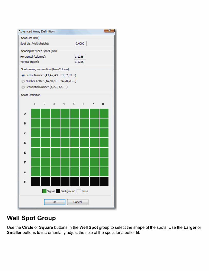
Well Spot GroupUse the Circle or Square buttons in theWell Spot group to select the shape of the spots. Use the Larger orSmaller buttons to incrementally adjust the size of the spots for a better fit.

Auto-Adjust GroupAutomatically moves the spots to the areas of fluorescence nearest them.
Background Group1. Use the controls in the Background group to specify the type of background. You can choose None,
Array, Average,Median, or User-Defined.
2. Select Array to open the Spots Definition grid on the Advanced Array Definition menu (see Spot Lay-out Group above for how to access the full menu). Choose the spot or spots to be designated as back-ground by clicking on each to toggle between Signal, Background, and None.
3. Select Average orMedian to open the Background menu. Here you can select the area around eachspot to use as background and the size of the area.
If you select User-Defined, you will need to assign spots for the background.
4. Click the Background button and select User-Defined from the drop-down menu.

5. Select a spot by clicking on the spot. The selected spot will have a dashed border. To select multiplespots, click and drag a bounding box around the spots or hold down the Ctrl key while clicking oneach spot.
6. Click Assign and all selected spots will be assigned as background spots. Note: Any spots that werepreviously assigned as background spots are automatically unassigned.
7. To unassign any spots, select the spot or spots (see step 2 above) and click Unassign.
Show GroupUse the controls in the Show group to specify what to display on the image. You can display Spots, Labels,Quantification, Grid Border, and Local Background (see Show Group for further details).
The check boxes are toggles. Click to check the box; click again to uncheck the box.

Grid AnalysisWhen an image with a Grid Analysis is the current image, the Grid Analysis Tab is shown on the ribbon.
Grid GroupA grid is placed on the image based on the last used settings when a Grid Analysis is applied.
1. Click the Redraw Boundary button and click and drag a bounding box on the image to draw a newgrid. Adjust the grid by selecting the bounding box and dragging the green arrows on each side. Movethe entire grid by dragging the double arrows that appear when hovering on the image.
2. Adjust the number of rows and columns by entering new values or using the up or down arrows toincrementally increase or decrease the number of rows or columns.
3. Click on the Grid Template button to choose, save, or delete a template that determines the Grid,Spot, and Background method settings. Note: Templates are useful for quickly selecting the settingsthat are commonly used, however, you do not need to use a template to set up a Grid Analysis.
4. The Grid Template button resets to Custom when any of the Grid, Spot, or Background method set-tings are changed. To save the current settings to a new template, click the Grid Template button andchoose Save Current Template from the drop-down menu.

5. Enter a name for the new template and click OK.
6. Click on the small arrow at the right edge of the Grid Group to open the Advanced Grid Definitionmenu where you can set the spot size and the spacing between spots numerically.
Spot GroupUse the Circle or Square buttons in the Spot group to select the shape of the spots. Use the Larger orSmaller buttons to incrementally adjust the size of the spots for a better fit.
Auto-Adjust GroupAutomatically moves the spots to the areas of fluorescence near them.
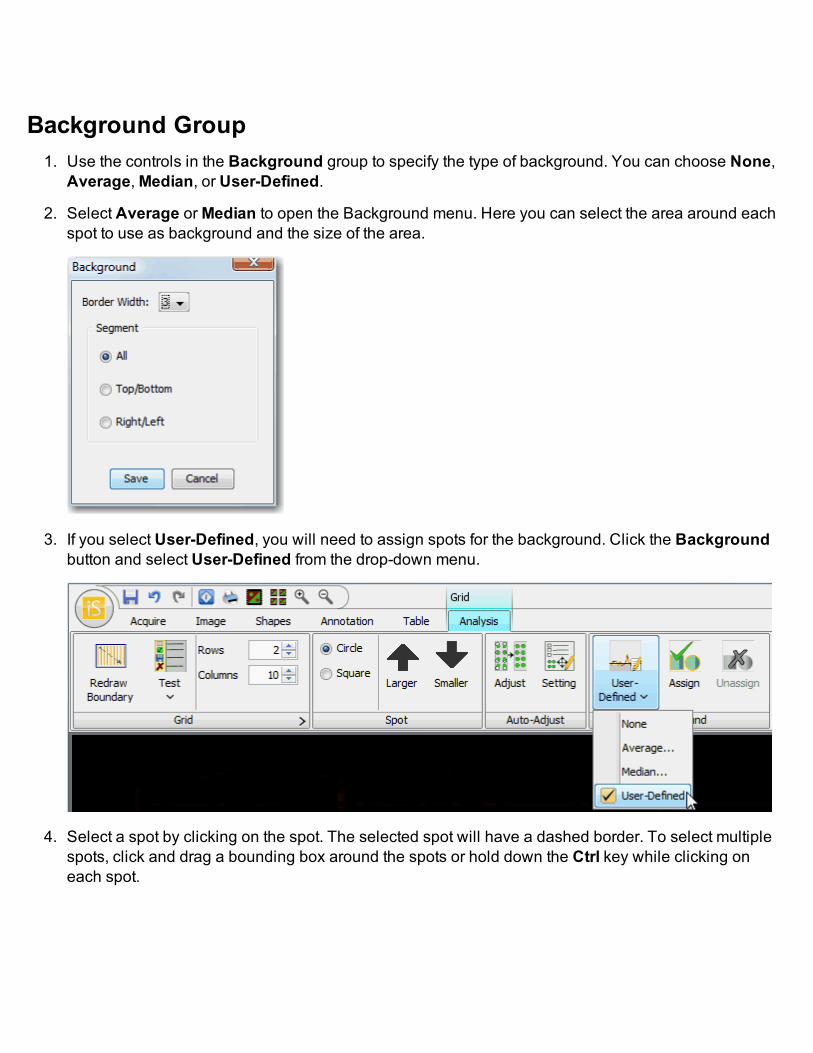
Background Group1. Use the controls in the Background group to specify the type of background. You can choose None,
Average,Median, or User-Defined.
2. Select Average orMedian to open the Background menu. Here you can select the area around eachspot to use as background and the size of the area.
3. If you select User-Defined, you will need to assign spots for the background. Click the Backgroundbutton and select User-Defined from the drop-down menu.
4. Select a spot by clicking on the spot. The selected spot will have a dashed border. To select multiplespots, click and drag a bounding box around the spots or hold down the Ctrl key while clicking oneach spot.

5. Click Assign and all selected spots will be assigned as background spots. Note: Any spots that werepreviously assigned as background spots are automatically unassigned.
6. To unassign any spots, select the spot or spots (see step 4 above) and click Unassign.
Show GroupUse the controls in the Show group to specify what to display on the image. You can display Spots, Labels,Quantification, Grid Border, and Local Background (see Show Group for further details).
The check boxes are toggles. Click to check the box; click again to uncheck the box.

Grid Array AnalysisWhen an image with a Grid Array Analysis is the current image, the Grid Array Analysis Tab is shown onthe ribbon.
Grid GroupA grid array is placed on the image based on the last used settings when a Grid Array Analysis is applied.
1. To draw a new grid array, click the Redraw Boundary and click and drag a bounding box on theimage.
2. To adjust the grid array, select the bounding box and drag the green arrows on each side. To move theentire grid array, drag the double arrows that appear when hovering on the image.
3. Adjust the number of rows and columns by entering new values or using the up or down arrows toincrementally increase or decrease the number of rows or columns.
4. Click on the Grid Array Template button to choose, save, or delete a template that determines theGrid, Array, Spot, and Background method settings. Note: Templates are useful for quickly selectingthe settings that are commonly used, however, you do not need to use a template to set up a GridArray Analysis.
5. The Grid Array Template button resets to Custom when any of the Grid, Array, Spot, or Back-ground method settings are changed. To save the current settings to a new template, click the GridArray Template button and choose Save Current Template from the drop-down menu.

6. Enter a name for the new template and click OK.
7. Click the small arrow at the right edge of the Grid group to open the Advanced Grid Definition menuwhere you can set the spacing between arrays numerically and choose how the arrays are named.
Array Group1. To adjust the number of rows and columns in the arrays, enter new values or use the up and down
arrows to incrementally increase or decrease the number of rows or columns. All of the arrays are

changed.
2. Use the Expand and Contract buttons to incrementally move the spots in the arrays.
3. Click the small arrow at the right edge of the Array Group to open the Advanced Array Definitionmenu where you can set the spot size, spacing between the spots in the arrays, and how the spots arenamed. Use the grid to define each spot as either Signal, Background, or None.

Spot GroupUse the Circle or Square buttons in the Spot group to select the shape of the spots. Use the Larger orSmaller buttons to incrementally adjust the size of the spots for a better fit.

Auto-Adjust GroupAutomatically moves the spots to the areas of fluorescence near them.
Background Group1. Use the controls in the Background group to specify the type of background. You can choose None,
Array, Average,Median, or User-Defined.
2. Select Array to open the Spots Definition grid on the Advanced Array Definition menu (see ArrayGroup above for how to access the full menu). Choose the spot or spots to be designated as back-ground by clicking on each to toggle between Signal, Background, and None.
3. Select Average orMedian to open the Background menu. Here you can select the area around eachspot to use as background and the size of the area.
4. If you select User-Defined, you will need to assign spots for the background. Click the Backgroundbutton and select User-Defined from the drop-down menu.

5. Select a spot by clicking on it. The selected spot will have a dashed border. To select multiple spots,click and drag a bounding box around the spots or hold down the Ctrl key while clicking on each spot.
6. Click Assign and all selected spots will be assigned as background spots. Note: Any spots that werepreviously assigned as background spots are automatically unassigned.
7. To unassign any spots, select the spot or spots (see step 5 above) and click Unassign.
Show GroupUse the controls in the Show group to specify what to display on the image. You can display Spots, Labels,Quantification, Grid Border, and Local Background (see Show Group for further details).
The check boxes are toggles. Click to check the box; click again to uncheck the box.

In-Cell Western AnalysisWhen an image with an In-Cell Western Analysis is the current image, the ICW Analysis Tab is shown onthe ribbon.
Plate GroupPlate TemplatesClick the Plate Template button to choose, save, or delete a template that determines the Plate andWellset-tings. Note: Templates are useful for quickly selecting the settings that are commonly used, however, you donot need to use a template to set up an ICW Analysis.
The Plate Template button resets to Custom when any of the PlateorWellmethod settings are changed.You can save the current settings to a new template.
1. Click the Plate Template button and choose Save Current Template from the drop-down menu.
2. Enter a name for the new template and click OK.

You can also delete a template from the list of available templates.
3. Click the Plate Template button and choose Delete Template to open the Delete Grid or Plate Tem-plate dialog.
4. Select the template to delete and click Delete. Note: You cannot delete the template currently in use.
5. Click Close.The template will be removed from the drop-down list.
Plate TypeChoose the type of plate from the Define Plate Type drop-down menu. You can choose from 6, 12, 24, 48,96, 384, or 1536 well configurations.

Adjust the size of the plate by selecting the bounding box and dragging the green arrows on each side.Move the entire plate by dragging the double arrows that appear when hovering on the image.
Well GroupUse the Circle or Square buttons in theWell group to select the shape of the wells. Use the Larger orSmallerbuttons to incrementally adjust the size of the wells for a better fit.
Definition GroupDefine the ICW Analysis with the controls in this group.
The first button toggles between None, 700, and 800.
Use the first button to select the channel used to normalize the results. The normalization channel oftendetects the total amount of protein while the other channel detects the protein of interest (e.g., phos-phorylated protein). In this example, the amount of phosphorylated protein in the other channel is adjusted

by the total amount of protein detected in the normalization channel. This method accounts for variation inprotein amount per well, resulting in better data.
Well TypesClick theWell Types button to open theWell Types dialog and assign each well as either Sample, 100%Std, Background, or None.


1. Select the type of well to mark by clicking the name in the Well Legend.
2. Click the well to assign the selected well type to that well.
3. Make multiple well assignments by dragging through the desired wells.
Note: If more than one Background well is designated, all Background wells will be averaged for the ICWcalculations. The same is true for 100% Standard wells.
Linked WellsClick the Linked Wells button to open the Well Links dialog. Select multiple rows or columns containingidentical samples to average the response of these samples.
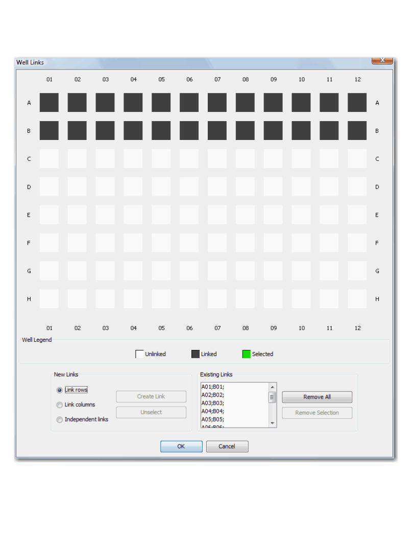

For example, if rows A and B are identically loaded, link the rows and the response from each pair of wellswill be averaged.
1. Drag through the rows to select them. They will be highlighted green.
2. Select Link rows.
3. Click Create Link. The linked rows will be black.
Each individual link (A01-B01, A02-B02, etc.) is listed in the Existing Links list. The analysis will averagethe linked wells in the Existing Links list and the averaged values will be used in ICW calculations ratherthan individual response values.
Individual wells can also be linked.
1. Click individual wells to select them. Selected wells are highlighted green.
2. Select Independent links, and click Create Link.
To dissolve a link, select the wells and click Unselect to change the well type from linked (green) tounlinked (white). Links can also be dissolved by clicking Remove All to remove all current row links, orselecting links in the link list and clicking Remove Selected. Shift+click and Ctrl+click are available formultiple selections.
Advanced ICW Definition1. For more options, click the arrow at the bottom right of the Definition group.
This opens the Expanded ICW Definition dialog.

Rows or columns can be analyzed individually. Only the background and 100% Standard well(s) inthat row or column will be used in the analysis.
2. Select the channels for the ICW analysis.
3. Select the column to use in the ICW analysis for the response value, such as Total.
Show GroupUse the controls in the Show group to specify what to display on the image. You can displayWells, Labels,Quantification, and Grid Border (see Show Group for further details).
The check boxes are toggles. Click to check the box; click again to uncheck the box.
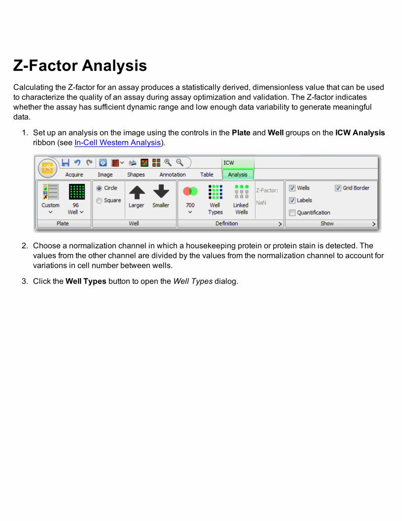
Z-Factor AnalysisCalculating the Z-factor for an assay produces a statistically derived, dimensionless value that can be usedto characterize the quality of an assay during assay optimization and validation. The Z-factor indicateswhether the assay has sufficient dynamic range and low enough data variability to generate meaningfuldata.
1. Set up an analysis on the image using the controls in the Plate andWell groups on the ICW Analysisribbon (see In-Cell Western Analysis).
2. Choose a normalization channel in which a housekeeping protein or protein stain is detected. Thevalues from the other channel are divided by the values from the normalization channel to account forvariations in cell number between wells.
3. Click theWell Types button to open theWell Types dialog.
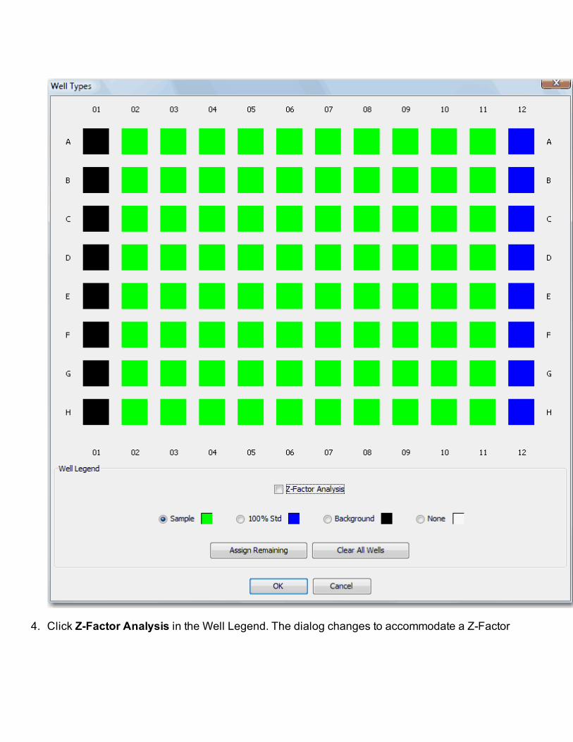
4. Click Z-Factor Analysis in the Well Legend. The dialog changes to accommodate a Z-Factor

Analysis.

5. Select the type of well to mark by clicking the name in the Well Legend.
6. Click the well to assign the selected well type to that well.
7. Make multiple well assignments by dragging through the desired wells.
8. Click OK.
The Z-factor calculation appears in the Definition group. For a description of the calculation, see CalculationDescriptions.
Advanced ICW DefinitionThe options in the Expanded ICW Definition dialog are not available for Z-factor analysis.
Show GroupUse the controls in the Show group to specify what to display on the image. You can displayWells, Labels,Quantification, and Grid Border (see Show Group for further details).
The check boxes are toggles. Click to check the box; click again to uncheck the box.

Small Animal Image AnalysisWhen an image with a Small Animal Image Analysis is the current image, the Small Animal Image Anal-ysis Tab is shown on the ribbon.
Shapes GroupShapes can be drawn on the image using the Draw Ellipse or Draw Freehand tools in the Shapes group.The Shape will be drawn in all channels that are displayed. Select the channel(s) to display and the displaycolor in the Image LUTs tab on the right. Note: If one channel is displayed in pseudo color, the other chan-nel must be gray scale with white shapes on black background.
l To draw an ellipse, click the Draw Ellipse tool. Click and drag from the center of the area of flu-orescence on the image to one corner.
l To draw a freehand shape, click the Draw Freehand tool. Click and drag around the area of flu-orescence on the image.
l Click Select to return to selection mode.
The Trim tool removes part of a Freehand or Auto shape to improve the fit of the shape to the area of flu-orescence. To use the Trim tool:
1. Select one channel to be displayed and disable the other channel in the Image LUTs tab on the right.
2. Select a drawn shape by clicking on it in selection mode. The outline of the shape will change to adotted line.
3. Click the Trim tool. Click and drag a line through the selected shape. The line must intersect the shapein two places.
4. Click on one side of the line to remove that side of the shape.

Background GroupNo background subtraction is applied until a shape is assigned as a background shape. To assign a shape:
1. Select a shape by clicking on it in selection mode. The outline of the shape will change to a dottedline. Note: To assign multiple shapes as background shapes, hold down the CTRL key and click oneach shape to select it.
2. Click on Assign Shape and all selected shapes will be assigned as background. For more infor-mation on how Signal is calculated using the Background, see Calculation Descriptions.
Auto Shape GroupThe Auto Shape tool creates a shape automatically that encloses fluorescence from irregularly shapedtumors or organs in images of small animals.
1. Select one channel to be displayed and disable the other channel in the Image LUTs tab on the righthand side.
2. After assigning a shape as background, click the Define New button to launch the Auto Shape tool.
3. Click the center of an area of fluorescence to create an Auto Shape.
4. Adjust the Std. Dev. Multiplier and Search Limit sliders in the Auto Shape group to interactivelychange the Auto Shape.
Standard Deviation MultiplierThe Standard Deviation Multiplier (Std. Dev. Multipler) is used in this equation to calculate the ThresholdValue:
Threshold Value = User-Defined Background + (Background Standard Deviation x Standard Deviation Mul-tiplier)
In general, increasing the Std. Dev. Multiplier increases the threshold and reduces the size of the AutoShape by excluding more pixels of lower intensity. Similarly, decreasing the Std. Dev. Multiplier increasesthe size of the Auto Shape.

Search LimitThe Search Limit controls the size of the image area that is searched to find a region of interest. The areasearched is a square centered on the mouse click such that the distance (pixels) from the center to the mid-point on any of the four line segments is equal to the Search Limit.
Setting the Search Limit to a smaller value can exclude unwanted fluorescence nearby, confining the AutoShape to the region of interest. Setting the Search Limit too low, however, could result in edges where thesearch area intersects the fluorescence in the region of interest.
Note: Search Limit is measured in pixels, so images scanned at higher resolution (smaller distancebetween data points) require higher search limits to cover the same image area.

Annotation TabThe Annotation tab is used to change text properties of lanes, bands, shapes as well as text annotation dis-played on the image.
The Annotation ribbon has controls that operate on selected "features" and added annotation. The lastused values (e.g., color and size) are used when any shape, band, or lane is created from the Analyze Tab.
When the font family, font size, or font style (bold or italic) are changed, all selected features will display thenew attribute. When an attribute is changed, it is not displayed on unselected annotation.
If multiple selections have different text attributes, the attribute is shown in the text control as an empty selec-tion.
The Bold and Italic font buttons are toggles that display the current style of the selected text. If multiple fea-tures are selected with different styles, pressing the Bold button removes the bold attribute from all selectedtext. Pressing the Bold button again, sets all text to be bold. Likewise, the Italic button sets all text to beitalic. Pressing the Italic button a second time causes all selected text to no longer display as italic.
The Edit Text button is used to change annotation text.

Adding TextSet the Text AttributesBefore you add the text you may want to specify the color, font, and size of the annotation. You can also dothis after you've added the text by selecting the text and then changing the attributes.
Use the controls in the Font group of the Annotation ribbon to specify the text properties.
l To specify the Font, use the drop-down menu and select the font from the list.
l To specify the Font size, use the drop-down menu and select the size from the list.
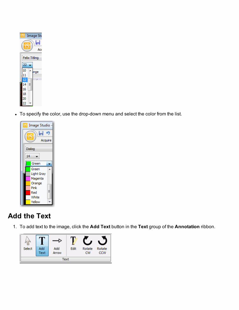
l To specify the color, use the drop-down menu and select the color from the list.
Add the Text1. To add text to the image, click the Add Text button in the Text group of the Annotation ribbon.

2. Click the spot on the image where you want to add the text. The Text Properties dialog is displayed.
3. In the Text field, type the text that you want to add to the image.
4. In Annotation Type, click the check box if you want to include a border around the text.
5. Click OK. The text is added to the image.
Reposition the TextAfter you have added the text, you may want to adjust its placement -- move it up or down or to another spoton the image.
1. Click the Select button and select the text. Note: If the text is close to a lane or a band, the easiest wayto select the text is to use the cursor to drag a small box through the center of the text.
2. The text will be boxed with a dotted line, and the cursor changes to four arrows.
3. Use the mouse or the direction arrows on your keyboard to move the selected text in any direction.
4. When the text is where you want it, click anywhere else on the image to de-select the text.

Edit the TextYou can change the text font, the font size, and the font color of selected text. You can also change font prop-erties: Bold and Italic, and increase or decrease the size in incremental steps using the Larger and Smallerbuttons. You can also edit the words.
1. Click the Select button and select the text that you want to edit.
2. Click the Edit Text button in the Text group of the Annotation ribbon.
The Text Properties dialog is displayed with the wording of the selected text displayed.
3. Edit the text. You can type over the selected text, or you can delete the selected text first.
4. Click OK. The revised text replaces the text on the image.

5. Click anywhere else on the image to de-select the text when you have finished.
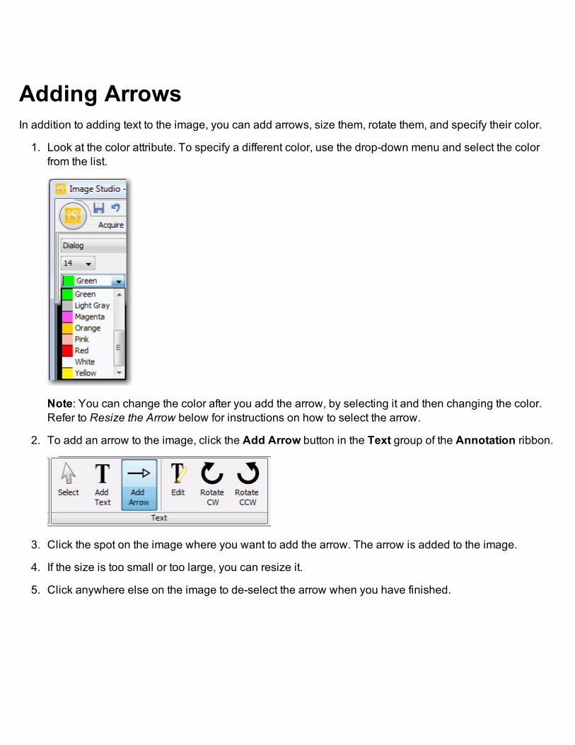
Adding ArrowsIn addition to adding text to the image, you can add arrows, size them, rotate them, and specify their color.
1. Look at the color attribute. To specify a different color, use the drop-down menu and select the colorfrom the list.
Note: You can change the color after you add the arrow, by selecting it and then changing the color.Refer to Resize the Arrow below for instructions on how to select the arrow.
2. To add an arrow to the image, click the Add Arrow button in the Text group of the Annotation ribbon.
3. Click the spot on the image where you want to add the arrow. The arrow is added to the image.
4. If the size is too small or too large, you can resize it.
5. Click anywhere else on the image to de-select the arrow when you have finished.
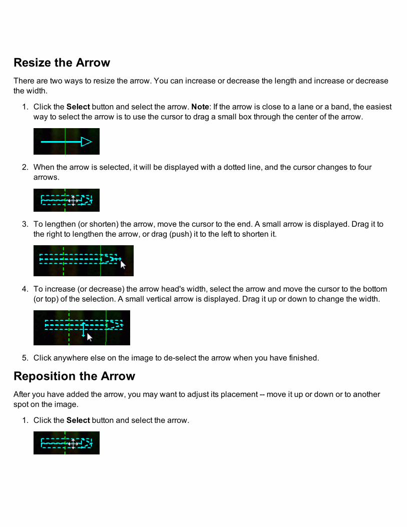
Resize the ArrowThere are two ways to resize the arrow. You can increase or decrease the length and increase or decreasethe width.
1. Click the Select button and select the arrow. Note: If the arrow is close to a lane or a band, the easiestway to select the arrow is to use the cursor to drag a small box through the center of the arrow.
2. When the arrow is selected, it will be displayed with a dotted line, and the cursor changes to fourarrows.
3. To lengthen (or shorten) the arrow, move the cursor to the end. A small arrow is displayed. Drag it tothe right to lengthen the arrow, or drag (push) it to the left to shorten it.
4. To increase (or decrease) the arrow head's width, select the arrow and move the cursor to the bottom(or top) of the selection. A small vertical arrow is displayed. Drag it up or down to change the width.
5. Click anywhere else on the image to de-select the arrow when you have finished.
Reposition the ArrowAfter you have added the arrow, you may want to adjust its placement -- move it up or down or to anotherspot on the image.
1. Click the Select button and select the arrow.

2. Use the mouse or the direction arrows on your keyboard to move the selected arrow in any direction.
3. Click anywhere else on the image to de-select the arrow when you have finished.
Rotate the Arrow1. Click the Select button and select the arrow.
2. Click one of the Rotate buttons in the ribbon (Rotate CW or Rotate CCW).
3. Click once to rotate 45°; click twice to rotate 90°.
4. Click anywhere else on the image to de-select the arrow when you have finished.
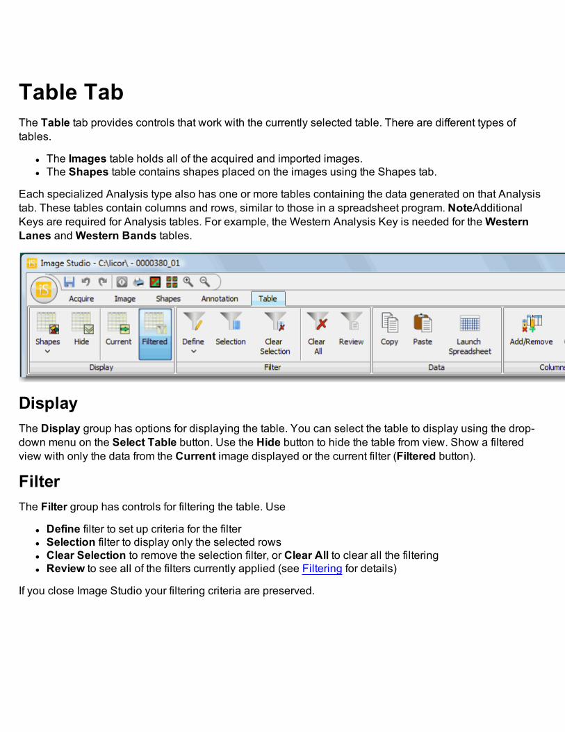
Table TabThe Table tab provides controls that work with the currently selected table. There are different types oftables.
l The Images table holds all of the acquired and imported images.l The Shapes table contains shapes placed on the images using the Shapes tab.
Each specialized Analysis type also has one or more tables containing the data generated on that Analysistab. These tables contain columns and rows, similar to those in a spreadsheet program. NoteAdditionalKeys are required for Analysis tables. For example, the Western Analysis Key is needed for theWesternLanes andWestern Bands tables.
DisplayThe Display group has options for displaying the table. You can select the table to display using the drop-down menu on the Select Table button. Use the Hide button to hide the table from view. Show a filteredview with only the data from the Current image displayed or the current filter (Filtered button).
FilterThe Filter group has controls for filtering the table. Use
l Define filter to set up criteria for the filterl Selection filter to display only the selected rowsl Clear Selection to remove the selection filter, or Clear All to clear all the filteringl Review to see all of the filters currently applied (see Filtering for details)
If you close Image Studio your filtering criteria are preserved.

DataThe Data group has commands for copying and pasting data between the table and other programs, suchas Microsoft Excel. Use
l Copy to copy selected rows from the table onto the clipboard to paste into another programl Paste to paste data from the clipboard that was copied from other programsl Launch Spreadsheet to open a spreadsheet program, such as Excel, with the selected rows of thetable in it (see Working with Table Data for details)
ColumnsThe Columns group has commands for adding and removing columns and for customizing some of the col-umn names. Some columns are specific to the table and some can be shared across tables. (See thedescription of each table type for more information about the columns available.)

Images TableThe Images Table contains a number of default columns that are pertinent to Images. Additional columnsare available in the Image Columns dialog. Click the Images tab at the lower left of the table to display theImages table.
The table can be filtered to display only the images of interest (see Filtering).
Adding or Removing ColumnsYou can add and remove columns in the Images table.
1. Click the Images tab at the lower left of the table.
2. Click the Add/Remove button in the Columns group of the Table ribbon. The Image Columns dialogis displayed.

3. Check (click) the columns that you want to include (click again to uncheck), and click Save when youhave finished.
Customizing ColumnsThere are 3 columns that can be renamed (Custom Image Column 1, Custom Image Column 2, and CustomImage Column 3). The fields in these columns are editable fields in which you can add text, similar to theComment field.
To Customize (rename) the column:
1. Select the Images tab at the bottom left of the table.
2. Click the Customize button in the Columns group of the Table ribbon. The Custom Columns dialog isdisplayed.
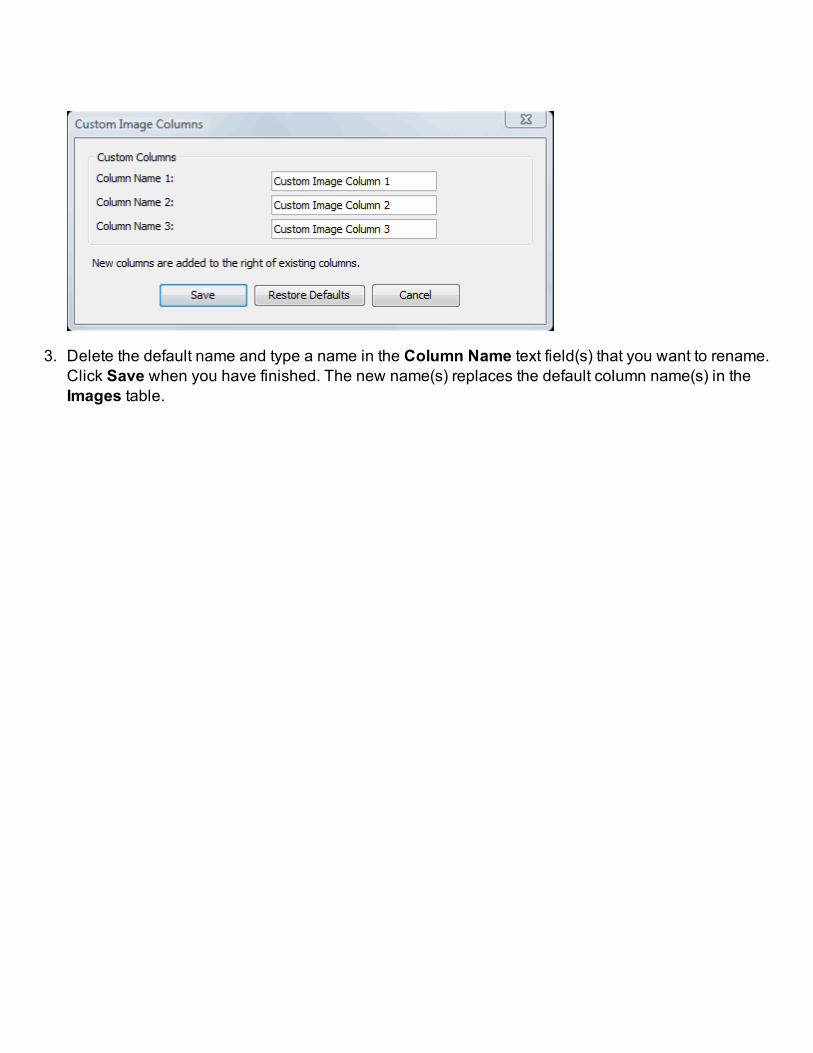
3. Delete the default name and type a name in the Column Name text field(s) that you want to rename.Click Save when you have finished. The new name(s) replaces the default column name(s) in theImages table.

Shapes TableThe Shapes Table contains a number of default columns that are pertinent to Shapes. Additional columnsare available in the Shapes Columns dialog. Click the Shapes tab at the lower left of the table to display theShapes table.
Adding or Removing ColumnsTo add or remove columns from the Shapes table:
1. Click the Shapes tab at the bottom left of the Table.
2. Click the Add/Remove button in the Columns group. The Shapes Columns dialog is displayed.

3. Check (click) the columns that you want to include (click again to uncheck), and click Save when youhave finished.
There are three columns (Custom Image Column 1, Custom Image Column 2, and Custom Image Column 3)that can be renamed in the Images Table (see Images Table). The fields in these columns are editable fieldsin which you can add text, similar to the Comment field.

Western Lanes TableTheWestern Lanes Table contains a number of default columns that are pertinent to Western Lanes. Addi-tional columns are available in the Lane Columns dialog. Click theWestern Lanes tab at the lower left ofthe table to display theWestern Lanes table.
Editing a Lane NameThe Lane Name column contains a default name for each lane, e.g., L01, L02, etc. You can edit a name byselecting the text in the Lane Name field and typing over the selected text with another name. The name youenter in the field will appear in the Profile title, the Single Image view, and in any report using the LaneName field.
Adding or Removing ColumnsTo add or remove columns from the Lanes table:
1. Click the Lanes tab at the bottom left of the Table.
2. Click the Add/Remove button in the Columns group. The Lane Columns dialog is displayed.

3. Check (click) the columns that you want to include (click again to uncheck), and click Save when youhave finished.
Customizing Western Lane ColumnsThere are two Western Lane columns that can be customized (CustomWestern Lane Column 1 and CustomWestern Lane Column 2. The fields in these columns are editable fields in which you can add text, similar tothe Comment field.
To customize the Western Lane column names:
1. Select theWestern Lanes tab at the bottom left of the table.
2. Click the Customize button in the Columns group of the Table ribbon. The CustomWestern Lane Col-umns dialog is displayed.

3. Delete the default name and type a name in the Column Name text fields that you want to rename.Click Save when you have finished. The new names replace the default column names in theWest-ern Lanes table.
Note: You can change these names later by clicking Customize again and either typing new namesor by clicking the Restore Defaults button which returns the names to the original default names (e.g.,CustomWestern Lane Column 1).

MPX Western Lanes TableThe MPX Western Lanes Table contains a number of default columns that are pertinent to MPX™WesternLanes. Additional columns are available in the Lane Columns dialog. Click the MPX Western Lanes tab atthe lower left of the table to display the MPX Western Lanes table.
Editing a Lane NameThe Lane Name column contains a default name for each lane, e.g., L01, L02, etc. You can edit a name byselecting the text in the Lane Name field and typing over the selected text with another name. The name youenter in the field will appear in the Profile title, the Single Image view, and in any report using the LaneName field.
Adding or Removing ColumnsTo add or remove columns from the MPX Lanes table:
1. Click the MPX Lanes tab at the bottom left of the Table
2. Click the Add/Remove button in the Columns group. The Lane Columns dialog is displayed.

Customizing Lane ColumnsThere are two Lane columns that can be customized (Custom MPX Western Lane Column 1 and CustomMPX Western Lane Column 2). The fields in these columns are editable fields in which you can add text,similar to the Comment field.
To customize the MPX Western Lane custom column name:
1. Select the MPX Western Lanes tab at the bottom left of the table.
2. Click the Customize button in the Columns group of the Table ribbon. The Custom Lane Columnsdialog is displayed.

3. Delete the default name and type a name in the Lane Column Name text field that you want to rename.Click Save when you have finished. The new names replace the default column names in the MPXWestern Lanes table.
Note: You can change these names later by clicking Customize again and either typing new namesor clicking the Restore Defaults button which returns the names to the original default names (e.g.,Custom MPX Western Lane Column 1).

DNA Gel Lanes TableThe DNA Gel Lanes Table contains default columns that are pertinent to DNA Gel Lanes. Additional col-umns are available in the Lane Columns dialog. Click the DNA Gel Lanes tab at the lower left of the table todisplay the DNA Gel Lanes table.
Editing a Lane NameThe Lane Name column contains a default name for each lane, e.g., L01, L02, etc. You can edit a name byselecting the text in the Lane Name field and typing over the selected text with another name. The name youenter in the field will appear in the Profile title, the Single Image view, and in any report using the LaneName field.
Adding or Removing ColumnsTo add or remove columns from the DNA Gel Lanes table:
1. Click the DNA Gel Lanes tab at the bottom left of the Table
2. Click the Add/Remove button in the Columns group. The Lane Columns dialog is displayed.

Customizing Lane ColumnsThere are two Lane columns that can be customized (Custom DNA Gel Lane Column 1 and Custom DNAGel Lane Column 2). The fields in these columns are editable fields in which you can add text, similar to theComment field.
To Customize the Lane custom column name:
1. Select the DNA Gel Lanes tab at the bottom left of the table.
2. Click the Customize button in the Columns group of the Table ribbon. The Custom Columns dialog isdisplayed.

3. Delete the default name and type a name in the Column Name text fields that you want to rename.Click Save when you have finished. The new names replace the default column names in the DNAGel Lanes table.
Note: You can change these names later by clicking Customize again and either typing new namesor by clicking the Restore Defaults button which returns the names to the original default names (e.g.,Custom DNA Gel Lane Column 1).

Western Bands TableTheWestern Bands Table contains a number of default columns that are pertinent to Western Bands. Addi-tional columns are available in the Band Columns dialog. Click theWestern Bands tab at the lower left ofthe table to display theWestern Bands table.
Adding or Removing ColumnsTo add and remove columns in the Western Bands table:
1. Select theWestern Bands tab at the lower left of the table.
2. Click the Add/Remove button in the Columns group of the Table ribbon. The Band Columns dialog isdisplayed.

3. Check (click) the columns that you want to include (click again to uncheck), and click Save when youhave finished.
There are two columns (CustomWestern Lane Column 1 and CustomWestern Lane Column 2) that can berenamed in the Western Lanes table (see Western Lanes Table). The fields in these columns are editablefields in which you can add text, similar to the Comment field.

MPX Western Bands TableThe MPX Western Bands Table contains a number of default columns that are pertinent to MPX™WesternBands. Additional columns are available in the Band Columns dialog. Click the MPX Western Bands tabat the lower left of the table to display the MPX Western Bands table.
Adding or Removing ColumnsTo add and remove columns in the MPX Western Bands table:
1. Select the MPX Western Bands tab at the lower left of the table.
2. Click the Add/Remove button in the Columns group of the Table ribbon. The Band Columns dialog isdisplayed.

3. Check (click) the columns that you want to include (click again to uncheck), and click Save when youhave finished.
There are two columns (Custom MPX Western Lane Column 1 and Custom MPX Western Lane Column 2)that can be renamed in the MPX Western Lanes table (see MPX Western Lanes Table). The fields in thesecolumns are editable fields in which you can add text, similar to the Comment field.

DNA Gel Bands TableThe DNA Gel Bands Table contains a number of default columns that are pertinent to DNA Gel Bands.Additional columns are available in the Band Columns dialog. Click the DNA Gel Bands tab at the lowerleft of the table to display the DNA Gel Bands table.
Adding or Removing ColumnsTo add and remove columns in the DNA Gel Bands table:
1. Select the DNA Gel Bands tab at the lower left of the table.
2. Click the Add/Remove button in the Columns group of the Table ribbon. The Band Columns dialog isdisplayed.

3. Check (click) the columns that you want to include (click again to uncheck), and click Save when youhave finished.
There are two columns (Custom DNA Gel Lane Column 1 and Custom DNA Gel Lane Column 2) that canbe renamed in the DNA Gel Lanes table (see DNA Gel Lanes Table). The fields in these columns are edi-table fields in which you can add text, similar to the Comment field.

Plate Wells TableThe Plate Wells Table contains a number of default columns that are pertinent to Plates. Additional col-umns are available in the Plate Columns dialog. Click the Plate Wells tab at the lower left of the table to dis-play the Plate Wells table.
The table can be filtered to display only the images of interest (see Filtering).
Adding or Removing ColumnsYou can add and remove columns in the Plate Wells table.
1. Click the Plate Wells tab at the lower left of the table.
2. Click the Add/Remove button in the Columns group of the Table ribbon. The Plate Columns dialog isdisplayed.
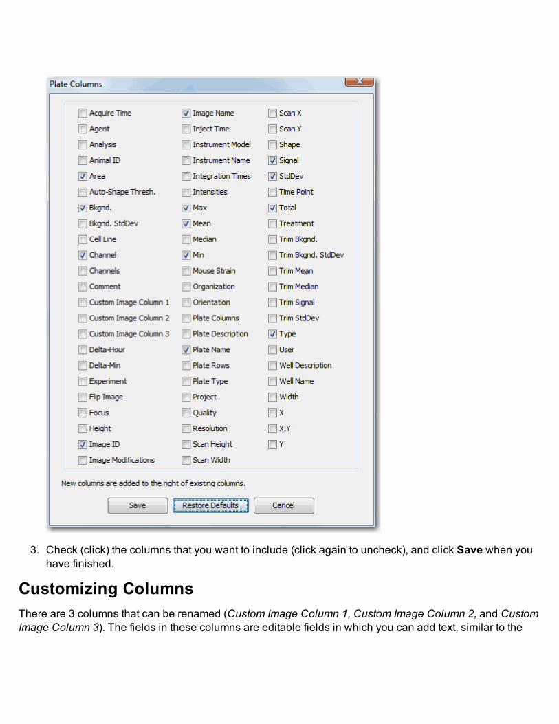
3. Check (click) the columns that you want to include (click again to uncheck), and click Save when youhave finished.
Customizing ColumnsThere are 3 columns that can be renamed (Custom Image Column 1, Custom Image Column 2, and CustomImage Column 3). The fields in these columns are editable fields in which you can add text, similar to the

Comment field.
To Customize (rename) the column:
1. Select the Images tab at the bottom left of the table.
2. Click the Customize button in the Columns group of the Table ribbon. The Custom Image Columnsdialog is displayed.
3. Delete the default name and type a name in the Column Name text field(s) that you want to rename.Click Save when you have finished. The new name(s) replaces the default column name(s).

Plate Array Spots TableThe Plate Array Spots Table contains a number of default columns that are pertinent to Plate Arrays. Addi-tional columns are available in the Plate Columns dialog. Click the Plate Array Spots tab at the lower left ofthe table to display the Plate Array Spots table.
The table can be filtered to display only the images of interest (see Filtering).
Adding or Removing ColumnsYou can add and remove columns in the Plate Array Spots table.
1. Click the Plate Array Spots tab at the lower left of the table.
2. Click the Add/Remove button in the Columns group of the Table ribbon. The Plate Array Columnsdialog is displayed.

3. Check (click) the columns that you want to include (click again to uncheck), and click Save when youhave finished.
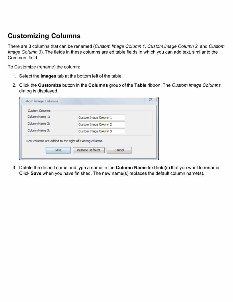
Customizing ColumnsThere are 3 columns that can be renamed (Custom Image Column 1, Custom Image Column 2, and CustomImage Column 3). The fields in these columns are editable fields in which you can add text, similar to theComment field.
To Customize (rename) the column:
1. Select the Images tab at the bottom left of the table.
2. Click the Customize button in the Columns group of the Table ribbon. The Custom Image Columnsdialog is displayed.
3. Delete the default name and type a name in the Column Name text field(s) that you want to rename.Click Save when you have finished. The new name(s) replaces the default column name(s).

Grid Spots TableThe Grid Spots Table contains a number of default columns that are pertinent to Grids. Additional columnsare available in the Grid Columns dialog. Click the Grid Spotstab at the lower left of the table to display theGrid Spots table.
The table can be filtered to display only the images of interest (see Filtering).
Adding or Removing ColumnsYou can add and remove columns in the Grid Spots table.
1. Click the Grid Spots tab at the lower left of the table.
2. Click the Add/Remove button in the Columns group of the Table ribbon. The Grid Columns dialog isdisplayed.

3. Check (click) the columns that you want to include (click again to uncheck), and click Save when youhave finished.
Customizing ColumnsThere are 3 columns that can be renamed (Custom Image Column 1, Custom Image Column 2, and CustomImage Column 3). The fields in these columns are editable fields in which you can add text, similar to the

Comment field.
To Customize (rename) the column:
1. Select the Images tab at the bottom left of the table.
2. Click the Customize button in the Columns group of the Table ribbon. The Custom Image Columnsdialog is displayed.
3. Delete the default name and type a name in the Column Name text field(s) that you want to rename.Click Save when you have finished. The new name(s) replaces the default column name(s).

Grid Array Spots TableThe Grid Array Spots Table contains a number of default columns that are pertinent to Grid Arrays. Addi-tional columns are available in the Grid Columns dialog. Click the Grid Array Spotstab at the lower left ofthe table to display the Grid Array Spots table.
The table can be filtered to display only the images of interest (see Filtering).
Adding or Removing ColumnsYou can add and remove columns in the Grid Array Spots table.
1. Click the Grid Array Spots tab at the lower left of the table.
2. Click the Add/Remove button in the Columns group of the Table ribbon. The Grid Array Columnsdialog is displayed.

3. Check (click) the columns that you want to include (click again to uncheck), and click Save when youhave finished.

Customizing ColumnsThere are 3 columns that can be renamed (Custom Image Column 1, Custom Image Column 2, and CustomImage Column 3). The fields in these columns are editable fields in which you can add text, similar to theComment field.
To Customize (rename) the column:
1. Select the Images tab at the bottom left of the table.
2. Click the Customize button in the Columns group of the Table ribbon. The Custom Image Columnsdialog is displayed.
3. Delete the default name and type a name in the Column Name text field(s) that you want to rename.Click Save when you have finished. The new name(s) replaces the default column name(s).

Grid SheetThe Grid Sheet tab appears at the bottom of the application window when a Plate, Plate Array, Grid, GridArray, or In-Cell Western Analysis is applied. Click on the tab to view the Grid Sheet.


Choose the value to display from the Field: drop-down menu.
Select the channel from the Channel: drop-down menu.

Working with Table DataThe Data group has commands to Copy selected rows from the table onto the clipboard for pasting intoother programs and to Paste the contents of the clipboard into the table. You can also select rows of thetable and launch a spreadsheet containing the selected rows of the table.
CopyThe Copy button copies to the clipboard the selected rows of the table view in the current order. If you wantall visible rows from the table, CTRL-A will select them all, or click the Select All button in the upper leftcorner of the table . Column headings are included.
1. Select the Table you want to work with.
2. Select one or more rows in the table. (Press CTRL-A to select them all, including the column head-ings, or click the Select All button.)
3. Click Copy or press CTRL-C on your keyboard. This copies the selection to the clipboard. You cannow paste the rows with the column headings in another program.
PasteThe Paste button pastes data from the clipboard down a table column starting at the current selection.
1. In the selected table, select any editable row or column.
2. Click Paste or press CTRL-V on your keyboard. This adds the rows from the clipboard in the selectedcolumn beginning with the selected row. Each entry in the paste buffer fills one row in the table view.Rows are filled starting with the selected row down one row per entry until reaching the last row in thetable view.
l If there are fewer entries in the paste buffer than remaining rows in the table view, all the entries in thepaste buffer are used, but all the rows may not be filled with new entries.
l If there are more entries in the paste buffer than remaining rows in the table view, the new entries arepasted into the selected column beginning at the selected row with a new entry in each subsequentrow until the end of the table view is reached. A warning message displays stating that some entries inthe paste buffer are discarded.
When the paste with multiple entries in the clipboard function is used on tables outside of the Images Tableon an Images Table column, all rows of this column will be the same. All values in this column will have thevalue of the last row filled in with this paste operation. This is because only one value is applied to this col-umn of the Images Table for a given Image ID. Since the non-image table is only of one Image ID, all rowsof any Image Table column are the same.

Launch SpreadsheetThis feature differs from Export Table on the Application menu in that instead of saving it to a file whichyou can open later outside of Image Studio, it saves the file and opens it while you have the table viewopen.
1. Select the rows that you want exported to a spreadsheet.
2. Click the Launch Spreadsheet button to create an Excel (*.xls) file containing the selected rows of thetable view in the current order.
3. If you have Excel on your computer, or another spreadsheet program that can open .xls files, the pro-gram is launched. First you will be prompted for a name. You can accept the default, or change thename and location. The program then opens.
Note: If you do not have an Excel or compatible program installed, you will get a message that an appli-cation to read Excel files must be installed before using this feature. You must also set the file association toopen the application for files with the .xls extension (this is done in theWindows Control Panel –> DefaultPrograms –>Set Associations dialog).
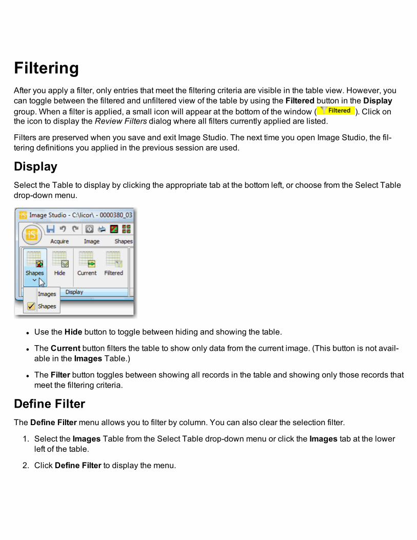
FilteringAfter you apply a filter, only entries that meet the filtering criteria are visible in the table view. However, youcan toggle between the filtered and unfiltered view of the table by using the Filtered button in the Displaygroup. When a filter is applied, a small icon will appear at the bottom of the window ( ). Click onthe icon to display the Review Filters dialog where all filters currently applied are listed.
Filters are preserved when you save and exit Image Studio. The next time you open Image Studio, the fil-tering definitions you applied in the previous session are used.
DisplaySelect the Table to display by clicking the appropriate tab at the bottom left, or choose from the Select Tabledrop-down menu.
l Use the Hide button to toggle between hiding and showing the table.
l The Current button filters the table to show only data from the current image. (This button is not avail-able in the Images Table.)
l The Filter button toggles between showing all records in the table and showing only those records thatmeet the filtering criteria.
Define FilterThe Define Filtermenu allows you to filter by column. You can also clear the selection filter.
1. Select the Images Table from the Select Table drop-down menu or click the Images tab at the lowerleft of the table.
2. Click Define Filter to display the menu.

3. Select a column name from the button drop-down to display the Define Filter dialog. This exampleshows the choices for the Analysis column.

4. Click (check) the analysis types to include in the filter. Filters from multiple columns can be active atthe same time.
Note that check marks indicate all of the filters that are currently defined. Multiple active filters are log-ically added together — the rows displayed are the intersection of the rows that are displayed by eachof the filters individually.
SelectionThe Selection filter creates a filter that displays only the currently selected rows in the table.
Clear SelectionThe Clear Selection button erases the Selection filter, but leaves other defined filters in place.
Clear AllThe Clear All button erases all existing filters so that a new filter (or set of filters) can be created.
ReviewClick the Review button to display a list of all filters currently applied in the table.

Exporting DataYou can export the data from any table to an Excel spreadsheet (or Excel-compatible spreadsheet). You canexport the entire selected table or selected rows in the table.
1. Click one of the Table tabs at the lower left of the table.
2. If you want to export selected rows, select the rows that you want to include.
3. Open the Application menu.
4. Click the Exportmenu and expand the Table submenu. Choose whether to include All Rows inTable or Selected Rows in Table. In this example the Images Export Table dialog is displayed (if youselected a Shapes table, for example, the Shapes Table Export dialog would display).

5. You can accept the default name, or change the name and location. See Building File Names UsingColumn Fields for information about using column fields in file names.
6. Choose Excel 97-2003 Workbook (*.xls) or Tab Delineated File (.txt) from the Files of type drop-downmenu.
7. Click Save and the .xls (or .txt) report is saved.
8. To view the report, navigate to the folder where you saved the file using Windows Explorer and openthe .xls file using your spreadsheet program or the .txt file in a text editor (Notepad, for example).
Note: If you saved to an .xls file and do not have Excel or a compatible program installed, you will geta message that an application to read Excel files must be installed before using this feature. You mustalso set the file association to open the application for files with the .xls extension (this is done in theWindows Control Panel –> Default Programs –> Set Associations dialog).
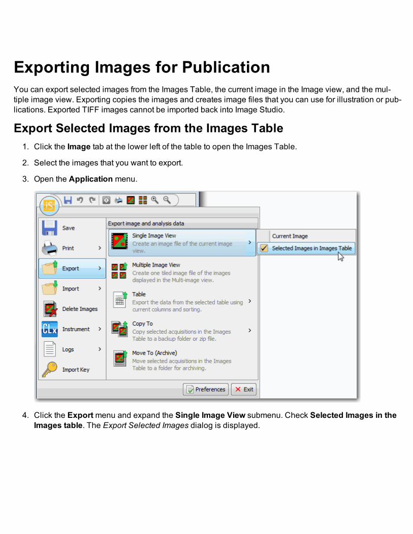
Exporting Images for PublicationYou can export selected images from the Images Table, the current image in the Image view, and the mul-tiple image view. Exporting copies the images and creates image files that you can use for illustration or pub-lications. Exported TIFF images cannot be imported back into Image Studio.
Export Selected Images from the Images Table1. Click the Image tab at the lower left of the table to open the Images Table.
2. Select the images that you want to export.
3. Open the Application menu.
4. Click the Exportmenu and expand the Single Image View submenu. Check Selected Images in theImages table. The Export Selected Images dialog is displayed.

5. Check Overwrite existing files, or uncheck if you don't want the existing files to be overwritten.
6. Select the Publication Resolution and the Image Format. If the image is for viewing on a website orin email, choose 72 dpi and High Quality JPEG file or PNG file.
7. If you accept the default folder and name, the folder will be your current Work Area and the name ofeach image will be its Image ID with an extension indicating the File type, for example, Image_0000019_01.tif, Image_0000020_01.tif
8. If you want to change the default name or folder, click Edit Name to change the name; click Browse tonavigate to a different folder. See "Edit File Name," below for more information about using its dialog.
9. Click Save when you have finished.
Export Current Image1. Open the Application menu. Click the Exportmenu and expand the Single Image View submenu.
Check Current Image. The Export Current Image dialog is displayed.

2. Select the Size Priority.
l Select Inches to set the output size in inches when changing DPI. The output pixel count isedited when the inches value is changed.
l Select Pixels to set the output size in pixels when changing DPI. The output inches value isedited when the pixel count is changed.
l Click Reset Pixels or Reset Inches to return the Output to the Original Size.
3. Select the Publication Resolution and the Image Format. If the image is for viewing on a website orin email, choose 72 dpi and High Quality JPEG file or PNG file.
4. If you accept the default folder and name, the folder will be your current Work Area and the name will
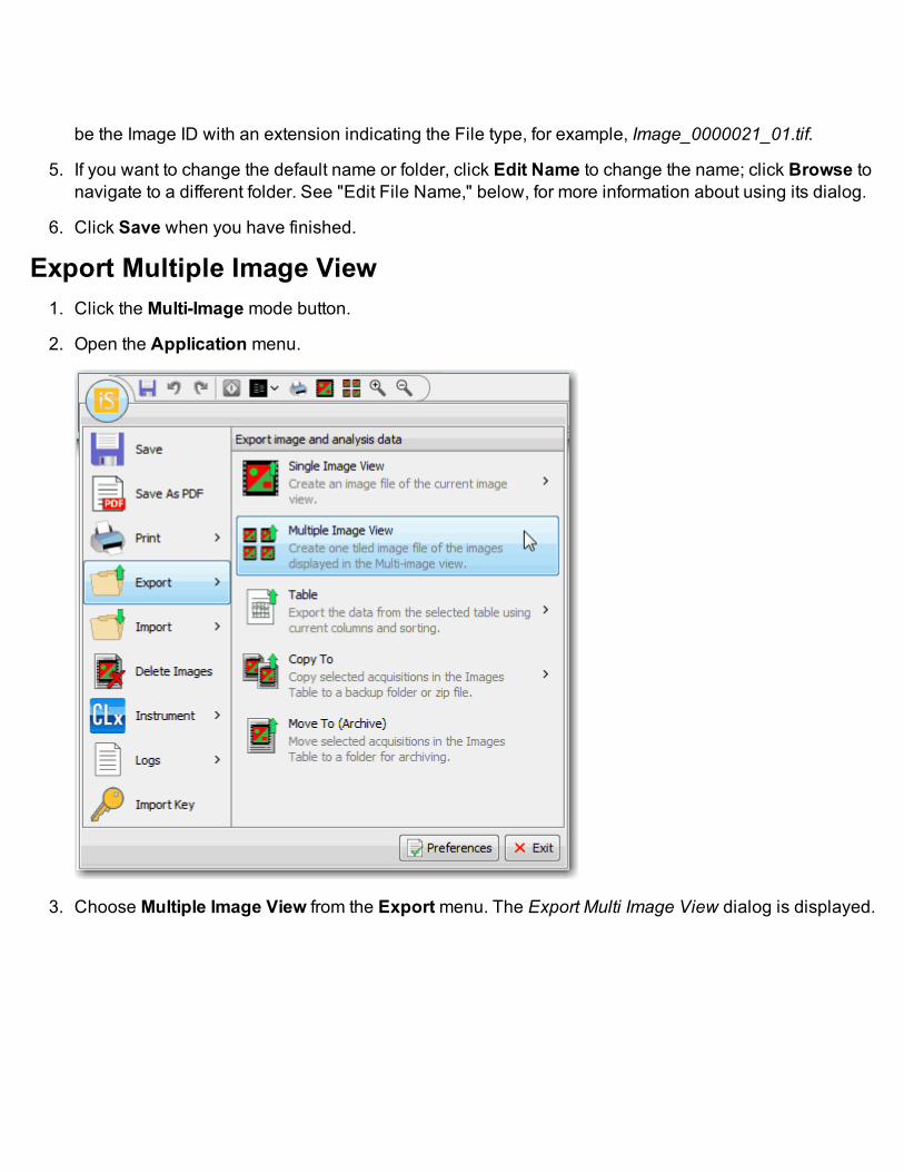
be the Image ID with an extension indicating the File type, for example, Image_0000021_01.tif.
5. If you want to change the default name or folder, click Edit Name to change the name; click Browse tonavigate to a different folder. See "Edit File Name," below, for more information about using its dialog.
6. Click Save when you have finished.
Export Multiple Image View1. Click the Multi-Image mode button.
2. Open the Application menu.
3. Choose Multiple Image View from the Exportmenu. The Export Multi Image View dialog is displayed.
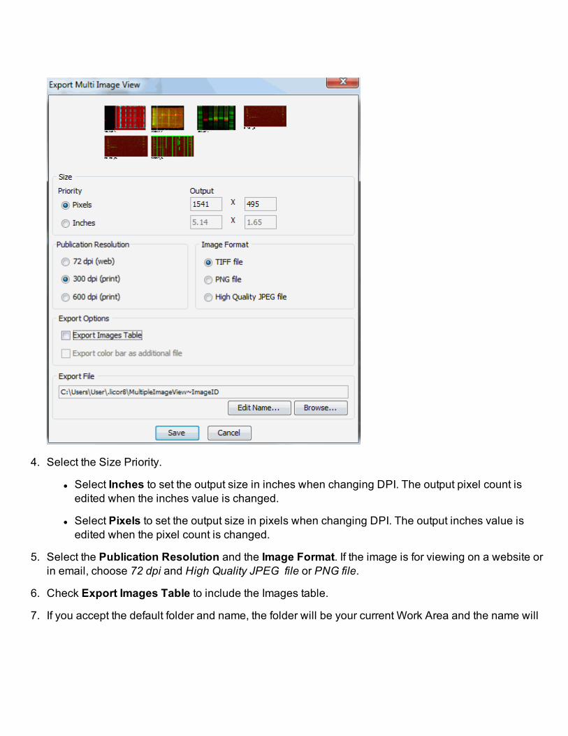
4. Select the Size Priority.
l Select Inches to set the output size in inches when changing DPI. The output pixel count isedited when the inches value is changed.
l Select Pixels to set the output size in pixels when changing DPI. The output inches value isedited when the pixel count is changed.
5. Select the Publication Resolution and the Image Format. If the image is for viewing on a website orin email, choose 72 dpi and High Quality JPEG file or PNG file.
6. Check Export Images Table to include the Images table.
7. If you accept the default folder and name, the folder will be your current Work Area and the name will

be MultipleImageView.
8. If you want to change the default name or folder, click Edit Name to change the name; click Browse tonavigate to a different folder. See "Edit File Name," below, for more information about using its dialog.
9. Click Save when you have finished.
Edit File NameThe Edit File Name dialog is displayed if you click Edit Name in the Export Selected Images or Export Cur-rent Image dialogs. The Edit File Name dialog provides a way to build a file name using selections from alist of the columns of the Images Table. The selections are inserted into File Name text field preceded by atilde (~).
1. Select a column field from the drop-down menu.
2. Click Insert. The field is added to the name in the File Name text field at the cursor location.
3. Repeat these steps to add more fields. Notice that the fields are preceded by a tilde (~).
4. To see what the filename will look like, view the Example File Name that is displayed in the dialog asyou add fields. Suggestion: Separate inserted fields with an underscore or space character to makethe fields readable.
5. Click OK when you have finished.
Note: If you are exporting selected images (more than one), be sure to include a unique value (we suggestImage ID). If you simply specify a filename, such as "My_Image~Date", as each file is created it will use thatname, thus overwriting the previously saved file.

See Building File Names with Column Name Fields for information about the Column fields and enteringthis information manually.

Printing ReportsReports and images can be printed from the Print dialog.
To access the Print options, open the Application menu and select Print.
There are three options on the Print secondary menu: Print, Quick Print, and Page Setup.
PrintThe Print dialog has controls for selecting the Images to print and the print format to use. You can alsoaccess the Page Setup dialog and specify the printer.

Print FormatThere are four pre-defined report formats:
l Single Image Per Page
l Multiple Images Per Page

l Table
l Lab Book
When you select a format, options specific to that format are displayed.
Print Destination1. Click Print or Print to PDF. If you choose Print to PDF, you will be prompted for a filename. A default
name is highlighted.
2. You can accept the default folder, WorkArea, and the default name, Report_~Date (which appends thedate). See example below to see the default filename as it appears in the Windows Explorer.

Or, navigate to another folder and/or enter a filename of your choice.
Quick PrintChoose Quick Print to print directly to the printer using all the previously specified print options.
Page SetupUse the Page Setup dialog to specify the page orientation, margins, and paper.

Print Single ImageThis report prints a single image on a page showing the current image or the images selected in the imagestable.
1. Open the Application menu and choose Print from the Print secondary menu. The Print dialog is dis-played.

2. Select Single Image Per Page.
3. Select whether to print the current Image or selected images in the images table.
4. Select the image size: Actual size or Scale to fit paper. Note: If you choose Actual size, and theimage is too large for the paper, it will be clipped.
5. You can optionally include the images table row and/or the image display values.
6. Click Print or Print to PDF (see Printing Reports for details on printing to a PDF file).

Print Multiple ImagesThis report prints the images in a tiled manner. The number of images across is defined by the numberacross value of the Multi-Image View Mode group in the Image tab.
1. Open the Application menu and choose Print from the Print secondary menu. The Print dialog is dis-played.

2. SelectMultiple Images Per Page.
3. You can optionally include the Images Table and/or the image display values.
4. Click Print or Print to PDF (see Printing Reports for details on printing to a PDF file).

Print TableThis report prints the selected table.
1. Open the Application menu and choose Print from the Print secondary menu. The Print dialog is dis-played.
2. Select Table. The name of the table currently selected in Image Studio appears on the right. To print a

different table, close this menu and go to the Table ribbon. Click the Select Table button and select adifferent table from the drop-down menu. Or, click the appropriate tab underneath the table to displaythe table you would like to print.
3. Select whether to print all rows or the selected rows in the table. The table data is determined by thecurrent column fields in use for the table. The sorting order is based on the table's current sorting selec-tion. Tables whose columns do not fit entirely on a page are continued on a new page at the samestarting location as the associated rows. Row numbers precede all other columns so that the rows forcolumns on multiple pages can be aligned.
4. Click Print or Print to PDF (see Printing Reports for details on printing to a PDF file).

Print Lab BookThe Lab Book is a custom defined report of images and/or table information. The Lab Book format uses sev-eral report building blocks. Although the predefined book cannot be changed, you can copy it and edit thecopy. You can print to a PDF file or your printer.
1. In Image Studio, select the images to include.
2. Open the Application menu and choose Print from the Print secondary menu. The Print dialog is dis-played.

3. Choose Lab Book from the Print dialog.
4. Choose which images to use. You can include multiple images that you have selected or the currentimage.

5. Click Print or Print to PDF (see Printing Reports for details on printing to a PDF file).

Build Custom Lab Book ReportYou can edit the Lab Book or you can make a copy of it and edit the copy.
1. Open the Application menu and choose Print from the Print secondary menu. The Print dialog is dis-played.
2. In the Print dialog, select Lab Book and click Copy. The Specify Custom Print Format Title dialog is

displayed.
3. Type a title for your lab book in the Title field and click OK. Your Western Lab Book is added to the list.

4. Select your lab book, and click Edit. The Print Format Builder dialog is displayed. (For a description ofall the fields available, see Lab Book Building Blocks.)

5. Select a field from the Available list, and click the Add button to move it to the In Use list.

6. To move the added field from the bottom to another position, select the field and click the Up button.To move another field down, select the field and click the Down button.
7. To move a field from the In Use to the Available list, select the field and click the Remove buttons.
8. Click Save when you have finished.

Lab Book Building BlocksFollowing is a list and description of all the building blocks available for designing a Lab Book.
Name Default Width DescriptionAcquisition Header Yes Full A three-line header, centered. Typically, this is the first
building block in the report. Line 1: Image ID, Line 2:optional user-specified table field used in the appli-cation title (or skipped if blank), and Line 3: current date.If you have a logo, add the logo information to theHeader 1. If a logo path is specified in the General Pref-erences, the image is rendered as a 2" x 1" image in theupper left corner of the header (see Preferences).
ConcentrationStandards-FullPage
Full Print the concentration standards for each channel in animage.
ConcentrationStandards-HalfPage
Half Print the concentration standards for each channel in animage.
Grid Sheet-All Chan-nels in Image
Yes Full Print the Grid Sheet for each channel of the image in ahorizontal table fashion. Print the same field/sub-grid asdisplayed in the Grid Sheet. If necessary, this sectionmay span more than one page.
Grid Sheet-Selected Channelin Image
Full Print the Grid Sheet for the image in a horizontal tablefashion. Print the same field/channel/sub-grid as dis-played in the Grid Sheet. If necessary, this section mayspan more than one page.
Image View-Fit FullPage
Full Print the current displayed image as seen in the appli-cation window. Scale the image to fit the current print-able area of the page. Print a color bar if the view is asingle channel. Print only the defined crop area if crop-ping is enabled.
Image View-Fit HalfPage
Yes Half Print the current displayed image as seen in the appli-cation window. Scale the image to fit half the pagewidth. Print a color bar if the view is a single channel.Print only the defined crop area if cropping is enabled.
Image View-Orig-inal Size-Full Page
Full Print the current displayed image as seen in the appli-cation window at 100% of the original size. Print a colorbar if the view is a single channel. Print only the definedcrop area if cropping is enabled.

Image View-Orig-inal Size-Half Page
Half Print the current displayed image as seen in the appli-cation window at 100% of the original size. Print a colorbar if the view is a single channel. If the image is large,it will not be clipped unless it is larger than the printablewidth, and the block printed to fit the remainder of thepage may be clipped. Print only the defined crop area ifcropping is enabled.
Images DisplayParameters-FullPage
Yes Full Print the image display values for the currently dis-played channels. Print one row per channel. Print chan-nel name, display color, LUT min value, LUT max value,and LUT K value.
Images DisplayParameters-HalfPage
Half Print the image display values for the currently dis-played channels. Print one row per channel. Print chan-nel name, display color, LUT min value, LUT max value,and LUT K value.
Images Table-Cur-rent Image-Vertical
Yes Half Print the currently displayed image from the Imagestable in vertical table fashion. Print one column for theheading names and another column for the table values.Use the fields displayed in the table.
Images Table-Cur-rent Image-Hor-izontal
Full Print the currently displayed image from the Imagestable in a horizontal fashion. Print one row for the head-ing names and another row for the table values. Use thefields displayed in the table.
Images Table-AllImages in Table
Full Print all images from the Images Table in horizontal fash-ion. Print one row for the heading names and anotherrow for each row in the Images Table. Use the fields dis-played in the table.
Images Table-Selected Images
Full Print currently selected images from the Images Table inhorizontal fashion. Print one row for the heading namesand another row for each selected image in the Table.Use the fields displayed in the table.
Lanes Table-AllLanes in Image
Yes Full Print all lanes from the Lanes Table in horizontal fash-ion. Print one row for the heading names and anotherrow for each row in the Lanes Table. Use the fields dis-played in the table. This may span more than onepage.A separate definition of fields is shown for WesternAnalysis, DNA Gel Analysis, and MPX Western Anal-ysis; however, this block will apply to whatever analysistype is currently being displayed.

Lanes Table-Selected Lanes inImage
Full Print currently selected lanes from the Lanes Table inhorizontal fashion. Print one row for the heading namesand another row for each row selected in the LanesTable. Use the fields displayed in the table. This mayspan more than one page. A separate definition of fieldsis shown for Western Analysis, DNA Gel Analysis, andMPX Western Analysis; however, this block will apply towhatever analysis type is currently being displayed.
Bands Table-AllBands in Image
Yes Full Print all bands from the Bands Table in horizontal fash-ion. Print one row for the heading names and anotherrow for each row in the Bands Table. Use the fields dis-played in the table. This may span more than one page.A separate definition of fields is shown for Western Anal-ysis, DNA Gel Analysis, and MPX Western Analysis;however, this block will apply to whatever analysis typeis currently being displayed.
Bands Table-Selected Bands inImage
Full Print currently selected bands from the Bands Table inhorizontal fashion. Print one row for the heading namesand another row for each row in the Bands Table. Usethe fields displayed in the table. This may span morethan one page. A separate definition of fields is shownfor Western Analysis, DNA Gel Analysis, and MPX West-ern Analysis; however, this block will apply to whateveranalysis type is currently being displayed.
Shapes Table-AllShapes in Table
Yes Full Print all shapes from the Shapes Table in horizontalfashion. Print one row for the heading names andanother row for each feature in the Shapes Table. Usethe fields displayed in the table. Reduce the font so thatall columns fit the available width. This may span morethan one page.
Shapes Table-Selected Shapes
Full Print currently selected shapes from the Shapes Tablein horizontal fashion. Print one row for the headingnames and another row for each feature in the ShapesTable. Reduce the font so that all columns fit the avail-able width. Use the fields displayed in the table. Thismay span more than one page.
Shapes Table-Selected Shapes inImage
Full Print currently selected shapes from the Shapes Tablefor the image in horizontal fashion. Print one row for theheading names and another row for each feature in theShapes Table. Reduce the font so that all columns fitthe available width. Use the fields displayed in the table.

This may span more than one page.Spots/Wells Table-All in Image
Yes Full Print all spots/wells from the Spots/Wells Table in hor-izontal fashion. Print one row for the heading namesand another row for each row in the Bands Table. Usethe fields displayed in the table. This may span morethan one page. A separate definition of fields is shownfor Grid, Grid Array, Plate, Plate Array, and ICW Anal-ysis; however, this block will apply to whatever analysistype is currently being displayed.
Spots/Wells Table-Selected in Image
Full Print the currently selected spots/wells from theSpots/Wells Table in horizontal fashion. Print one rowfor the heading names and another row for each row inthe Bands Table. Use the fields displayed in the table.This may span more than one page. A separate def-inition of fields is shown for Grid, Grid Array, Plate, PlateArray, and ICW Analysis; however, this block will applyto whatever analysis type is currently being displayed.

Band NormalizationNormalization is useful for using one channel to correct for loading variation between lanes. This value isalso displayed in the Normalization Channel column in the Images Table. (If this column is not in yourImages Table, see "Adding and Removing Columns" in the Images Table for instructions.)
The Lanes Table has a Normalization Factor column. (If this column is not in your Lanes Table, see "Add-ing and Removing Columns in the Lanes table for instructions.) If the lane has a single band in the Nor-malization Channel, the Normalization Factor is calculated by dividing the signal for this single band by themaximum signal of all singleton bands in the Normalization Channel. Otherwise the value is NaN. Thevalue will be identical for all channels within a lane.
The Normalized Signal column in the Bands Table is calculated as the Signal divided by the NormalizationFactor. (If this column is not in your Bands Table, see "Adding and Removing Columns" in the Bands Tablefor instructions.)

Building File Names Using Column FieldsThe Export Selected Images dialog has an Edit Name button that displays the Edit Name dialog allowingyou to include column name fields in the file name. You can also include column name fields in other exportdialogs by entering the column name fields manually.
The name that you enter must be preceded by a tilde for the field to be replaced by the current value. In theexample below, the user accepted the default file name, ImagesTableExport_~Date and appended a Timefield, preceded by a Tilde (~).
Use the following table to find the name(s) that you want to append to the file name.
To Use This Column Name Insert This Name Preceded by a Tilde (~) Description
Date Date Current date in the formatYYYY-MM-DD
Time Time Time in the format ofHHMMSS
Work Area Work Area Work Area folder name

To Use This Column Name Insert This Name Preceded by a Tilde (~) DescriptionImage ID ImageID
Values supplied from cur-rent acquisition
Image Name Image NameAcquire Time Time StampInstrument Name InstrumentNameChannels ChannelsIntegration Times IntegrationTimesResolution ResolutionFocus FocusPositionTime Point TimePointDelta-Min TimePointDeltaMinutesDelta-Hour TimePointDeltaHoursNormalization Channel NormalizationChannel<specified custom name> CustomField1<specified custom name> CustomField2<specified custom name> CustomField3Project ProjectUser UserAnalysis AnalysisType
Organization OrganizationName The organization spec-ified in Preferences
Animal ID AnimalID
Editable fields that can beincluded in the ImagesTable and values sup-plied by the user
Orientation OrientationTreatment TreatmentInject Time InjectTimeExperiment ExperimentComment AnimalCommentMouse Strain MouseStrainAgent AgentCell Line CellLine

Calculation DescriptionsIn the Tables there are columns that refer to calculations. When these columns are part of the table, thevalues are automatically calculated and reported in the table. Some columns are specific to one table andsome can be shared across tables. The Columns group has commands for adding and removing columns.For further instructions, select "Adding and Removing Columns" in the help section of any table type.
Below are detailed descriptions of the calculations in these columns. First, the terms used in these descrip-tions are defined.
Definitions of TermsShape— any area enclosed using the shape tools.
Pixel— the smallest area unit of an image that is measured with a single intensity value.
Signal intensity or intensity— signal counts measured in a single pixel per unit time.
Descriptions of the CalculationsArea— The area is the total number of pixels enclosed by a shape.
Bkgnd.— The background is the average intensity of the pixels selected as the background region.
Bkgnd. Std Dev— The background standard deviation is the standard deviation of all of the backgroundpixel intensities in a single channel.
Max— The maximum intensity is the highest pixel intensity within a shape. The maximum intensity valuedoes not have background intensity subtracted.
Mean— The mean is the sum of all of the pixel intensities for a shape divided by the total number of pixelsin a shape.
Min— The minimum intensity is the lowest pixel intensity within a shape. The minimum intensity value doesnot have background intensity subtracted.
Signal— The signal is the sum of the individual pixel intensity values (Total) for a shape minus the productof the average intensity values of the pixels in the background (Bkgnd.) and the total number of pixelsenclosed by the shape (Area). Signal = Total - (Bkgnd. x Area)
StdDev— The standard deviation of all of the pixel intensities for a shape.
Total— The total intensity is the sum of the individual pixel intensities for a shape.

Trim Bkgnd.— The trimmed background is the average intensity of the pixels selected as the backgroundregion. Note: the highest 5% count and lowest 5% count of the intensity pixel values of the background arediscarded.
Trim Bkgnd. StdDev— The trimmed background standard deviation is the standard deviation of all of thebackground pixel intensities in a single channel. Note: the highest 5% count and lowest 5% count of theintensity pixel values of the background are discarded.
Trim Mean— The trimmed mean is the sum of all of the pixel intensities for a shape divided by the totalnumber of pixels in a shape. Note: the highest 5% count and lowest 5% count are excluded from the inten-sity summation and pixel count.
Trim Signal— The trimmed signal is the sum of the individual pixel intensity values for a shape minus theproduct of the average intensity values of the pixels in the background (Bkgnd.) and the total number of pix-els enclosed by the shape. Note: The highest 5% count and lowest 5% count are excluded from the intensitysummation and the pixel count.
Trim StdDev— The trimmed standard deviation is the standard deviation of all of the pixel intensities for ashape. Note: the highest 5% count and lowest 5% count of the intensity pixel values of the shape are dis-carded.
In-Cell Western CalculationsBackground— Pixel intensities in all wells designated as Background in a channel are averaged, and theaverage is subtracted from the pixel intensities of wells in that channel that are designated as Sample.
Linked Wells— The pixel intensities from linked wells are averaged, and this average is used in the fol-lowing calculations for each of the linked wells.
ICW Relative— After background subtraction, all wells designated as Sample or 100% Standard in a chan-nel are divided by the intensity value of the well with the highest response. This well is given a value of 1.0,and the relative intensity values of the other wells will generally be between 0.0 and 1.0. Note Negative rel-ative intensities indicate the original intensity value was lower than the average background when the back-ground was subtracted.
If a normalization channel is selected, the intensity value of each well in the other channel is divided by therelative intensity value of the corresponding well in the normalization channel.
ICW % Response— After background subtraction and normalization (if used), all wells designated as Sam-ple are divided by the average of the wells designated as 100% Standard in that channel and multiplied by100 to give a percentage response to the control in the 100% Standard. Note: All ICW % Response valuesfor the normalization channel are reported as NaN.
ICW Std Dev— The ICW standard deviation is the standard deviation of the average of the pixel intensitiesfrom linked wells.
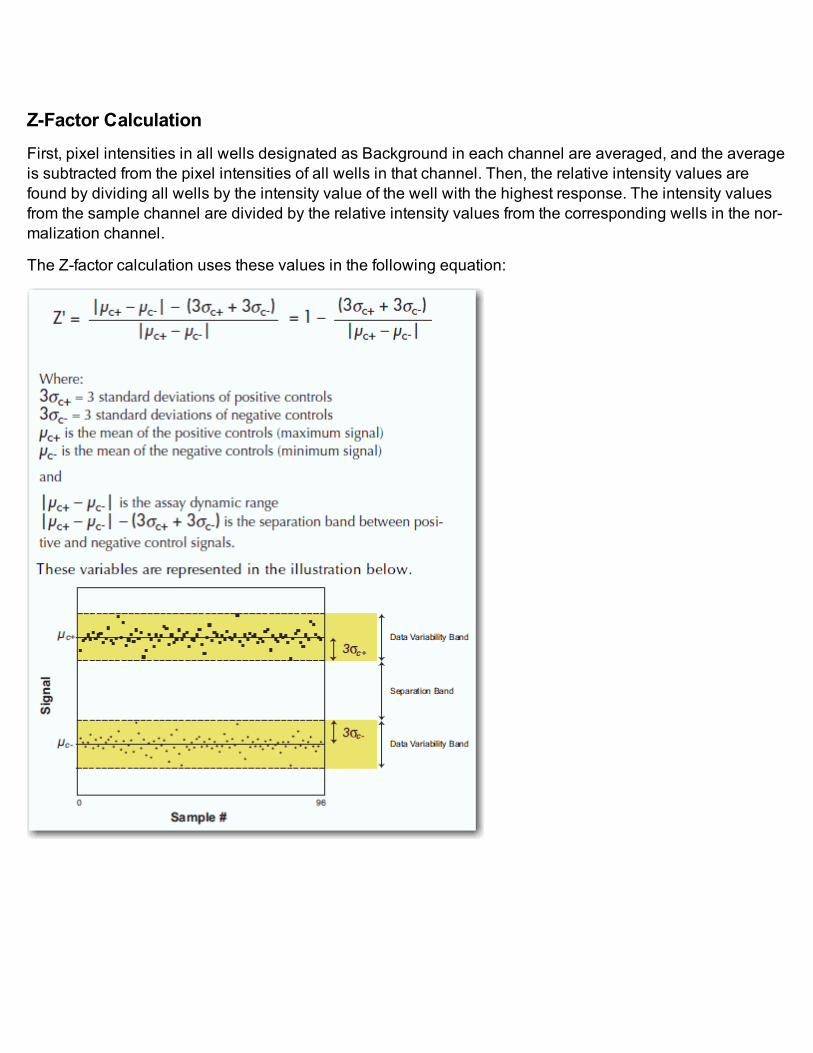
Z-Factor CalculationFirst, pixel intensities in all wells designated as Background in each channel are averaged, and the averageis subtracted from the pixel intensities of all wells in that channel. Then, the relative intensity values arefound by dividing all wells by the intensity value of the well with the highest response. The intensity valuesfrom the sample channel are divided by the relative intensity values from the corresponding wells in the nor-malization channel.
The Z-factor calculation uses these values in the following equation:
GlossaryAcquire: Obtaining an image, by instrument or by importing an image file.
Acquisition: Image and its Analysis.
Analysis Type: Can include Westerns, ICW, DNA Gels, and more. After specifying the Analysis type, theuser is presented with a predefined set of acquisition parameters and analysis.
Application Button: The large button in the upper left corner of the application window that contains amenu of operations that in some applications are most usually found on the File menu.
Background Type: Method of calculating background
Band: A feature in a lane that indicates detection of a protein or DNA.
Bands Table: A tabular view of values in the Band fields, both automatically and manually assigned.
Boundary: Outline of lanes area. To see the outline be sure that Boundary is checked in Show options.
Button: A small icon that issues a command when clicked.
Channel: A description of the method used to collect pixel values. The description is usually a single wordor number approximating either the emission and/or detection wavelengths or the detection method.
Columns: A set of values assigned to each image or feature. For example, Image columns for each Imageare viewed in the Images Table. Some values are automatically assigned during the acquisition processbased on acquisition parameters, (Resolution, offset, channels, date-time of acquisition, for the Image col-umns for example.) Other columns are manually assigned..
Comb: An apparatus used to form the wells in a gel. A setting for determining number of lanes in the West-ern MPX Analysis.
Ellipse: An elliptical shape, that can be quantified, drawn around some section of the image.
Export: A command on the Application menu as a way to copy or move images and data.
Feature: A box, circle or other shape drawn around some section of the image. This object is visible on theImage View and can be quantified.
Filters: Ways to restrict the Image Table view when many images are loaded into Image Studio.
Group: A group of related commands in a Task Tab or ribbon (e.g., the Filter group in the Table tab).
Image: The viewable result of the Acquire action. This also refers to the set of all individual channels and allanalysis and logs. An Image-ID, a unique number, is automatically assigned to each image as the result ofan acquisition.

Images Table: A tabular view of values in Image fields, both automatically and manually assigned.
Key Tip: Letter(s) and numbers for accessing commands using the keyboard. Pressing the ALT key acti-vates Key Tips.
Lab Book Report: A customized report of selected images and table data. This report is found on the Appli-cation menu's Print menu.
Lane: A group of bands visible in the image that have the same channel, sample, primary, secondary, andtertiary (if defined) attributes. In a Western, there is on lane per channel per well. In an MPX™Western,there is one lane per channel per MPX apparatus groove.
Lanes Table: A tabular view of values in the Lane fields, both automatically and manually assigned.
LUT: Lookup Table. Used to transform the raw pixel data from an image channel into a grayscale or colorfor display..
Marker: A mixture of labeled proteins or DNA having defined size. Also known as Sizing Standards.
Marker Lane: A lane that contains a marker.
Profile: Graphic display of a band or lanes showing pixel location and intensity.
Quick Access Toolbar: A group of buttons located to the right of the Application Button. Used to performcommon commands.
Rectangle: A rectangle shape that can be quantified, drawn around some section of the image.
Ribbon: An area at the top of the application window containing the Application Button, Quick Access Tool-bar, and a set of Task Tabs.
Shape: This describes the geometry of a feature. Examples are square, ellipse, polygon, auto, band.
Shapes Table: A tabular view of values in the Shapes fields, both automatically and manually assigned.
Task Tabs: A tab located in the Ribbon containing Groups. Command Tabs are always visible. The vis-ibility of Contextual Tabs is determined by the selection.
Title Bar: The bar above the application window that displays the name of the program and the currentimage.
Toolbar: A group of buttons.
Tooltip: Hover the mouse over a button or control in a dialog to display a brief explanation of the control.
Well: A depression used to contain a sample. In a Western or MPX Western, wells are created in the gel bythe comb. In a microplate, the wells are features of the plate.

Western: Western Blot. A method in molecular biology to detect a certain protein in a sample by using anti-body specific to that protein.